4. c generation algorithm and i shortest path problem · simplex method for solving large-sized...

4. Column Generation Algorithm and Indexed Shortest Path Problem 44

4. COLUMN GENERATION ALGORITHM ANDINDEXED SHORTEST PATH PROBLEM

This chapter and the next are concerned with the solution of the developed models

in practice. The discussion in this chapter focuses on the mathematical algorithm

proposed for solving the linear programming models LPIM and LPIM(TT) developed

in the last chapter. It begins with a discussion on the limitations of the standard

simplex method for solving large-sized linear programming problems. A Column

Generation Algorithm (CGA) is then adopted to exploit the special structure of the

model. In order to be consistent with other transportation models, an indexed-cost

minimum path problem, and its linearized version, are proposed, and a suitable

algorithm is then presented. The issues on how to implement the algorithm via a

computer code will be presented in the next chapter.

4.1 Limitations of the Standard Simplex Method

Despite its success in theoretical research and in practical application, the standard

simplex method is known to have certain limitations in solving large-sized linear

programming problems. For the linear programming models developed so far,

these limitations arise in the following aspects (Sivanandan 1991, Sherali et al.

1994a). 1) An explicit statement of the linear programming models LPI, LPIM, etc.,

requires the enumeration of all possible paths between each O-D pair ( , )i j OD∈ .

Although this is readily accomplished in theory, it is computationally prohibitive

except for small-sized networks. 2) In addition, excessive computer storage will be

necessary to store the path information as required by the simplex procedure. This

also leads to a limitation for large-sized networks. 3) As an alternative, one can


consider the explicit generation of only Dial’s (1971) “efficient” paths. However, an

example (Sivanandan 1991, Sherali et al. 1994a) shows the failure of this attempt to

produce acceptable solutions in certain cases. Another alternative is to use some

interior point algorithm, which is known to have polynomial-time complexity

(Bazaraa et al. 1990, 1993). Although these algorithms might reduce the total

number of iterations, they cannot overcome the other limitations mentioned above.

4.2 Decomposition Principle and Column GenerationTechnique

It is well known that the Dantzig-Wolfe decomposition technique, which is equivalent

to Benders’ partitioning and Lagrangian relaxation for linear programming (Bazaraa

et al., 1990), is often suitable for solving large-sized problems. The idea behind

these techniques is to convert the large problem into one or more appropriately

coordinated smaller problems of manageable size. When this principle is applied to

the revised simplex method, in which the columns of the linear program are

selectively generated, the procedure is known as a Column Generation Algorithm

(CGA) (Lasdon 1970).

The theoretical background of CGA may be illustrated as follows. Consider the

linear program

Minimize z c xjj

n

j==

∑1

[4.1a]

subject to A x bjj

n

j=

∑ =1

[4.1b]

x ≥ 0, [4.1c]

where Aj , j n b=1, , ,L and are m (<n)-dimensional vectors. Assume that there is a

basic feasible solution (BFS) xB available, with an associated basis matrix B and


cost coefficient cB . Then the simplex multiplier (dual vector) associated with this

basis is given by

π = −c BB1 . [4.2]

Now, if the reduced cost coefficients c Aj j− ≥π 0 for all of the nonbasic variables,

then the optimal solution of the linear program [4.1] is at hand. On the other hand, if

there is a k such that

π πA c A ck k j j j− = − >max 0, [4.3]

then the standard simplex method can be applied, by entering xk into the basis

through a pivot operation, and an adjacent (improved) basis can be found. For

large-sized problems, finding the maximum in [4.3] by computing each πA cj j−

may be computational expensive. In some cases, however, these columns can be

identified as vertices of another polytype s (Bazaraa et al. 1990, Ch7). In such a

case, the column to be entered into the basis can be chosen by solving the

following subproblem

.A j

maximum jS

CA −∈

π [4.4]

The solutions of the subproblem are then sent to the master problem for pivoting

and updating. These iterations continue until optimality (of the master problem) is

reached. Note that the above CGA cannot be directly applied to the linear

programming models formulated in the last chapter, and some modification is

necessary to perform this task.

4.3 Choice of a Starting Basic Feasible Solution

The following two sections will develop a column generation scheme for solving the

linear programming models established in the previous chapter. This section is

concerned with the starting basic feasible solution (BFS) used by various simplex


implementations. For the sake of simplicity, only the model LPIM defined in [3.14]

will be used for illustrative purposes. The other models are discussed in some

remarks.

Introducing slack variables sa in [3.14b] and ta in [3.14c] for a Av∈ , respectively,

the linear program [3.14] can be rewritten as

LPIM: Minimize ( , )

~i j O D

ijk

k

n

ijk

Ac x M e yij

v∈ =

∑ ∑ + ⋅1

[4.5a]

subject to vaaaakija

kij

ODji

n

k

Aafsyxpij

∈Λ+=−+∑ ∑∈ =

,)(),( 1

[4.5b]

vaaaakija

kij

ODji

n

k

Aaftyxpij

∈Λ+=+−∑ ∑∈ =

,)(),( 1

[4.5c]

0,0,0,0 ≥≥≥≥ tsyx , [4.5d]

where, the penalized travel time ~cijk is given by [3.14e].

To solve the linear program [4.5] by using a simplex-based method, a starting Basic

Feasible Solution (BFS) is needed. Depending on different viewpoints, the following

three approaches may be considered for determining a starting BFS.

1) By setting aa fy = and aaa ft Λ+= 2 , a starting BFS for solving [4.5] is already

at hand. Both the primal and the dual problems corresponding to this BFS are

very simple. The shortcoming of this choice of a starting BFS is that the

corresponding objective value is very high.

2) Since the high cost variable ay may be set to be zero for a Av∈ if and only if

],[ aaaa fff Λ+∈ , another choice of a starting BFS ( , , , ), ,x y s t a Aa a a a ∈

might be composed by using the following procedure. First, alter the flows on

some links so that the assigned flows f a Aa , ∈ , are conserved at each

intermediate node and are as “close” to the lower-cost interval ],[ aaa ff Λ+


as possible. Then find an O-D trip table on some possible paths so that the

assigned flows match with the balanced flows. Finally purify the feasible

solution obtained to a starting basic feasible solution (Bazaraa et al. 1990).

However, this three-step procedure for tracing a starting BFS could itself be

computational expensive, because of the possible occurrences of cyclic flows

that require the above balancing-assignment procedures to be performed

many times.

3) As an alternative, one may consider finding an O-D trip table first according to

some information of the observed flows. Then, by assigning this O-D table to

the corresponding paths, deleting the excess flows on links and setting the

artificial variable y and slacks s and t correspondingly, a feasible solution

can be obtained. Finally, by using the purification procedure, this feasible

solution can be purified to a “better” basic feasible solution. For the purpose of

finding a suitable feasible solution, the backtracing algorithm in the LP model

(Sherali et al. 1994a) may be used, with some modification based on the

following principles. 1) Preferably, alter the “flows” on those links having

“missing volumes”, whenever possible, rather than on other links. 2)

Preferably, alter the slacks sa or ta , whenever possible, rather than increase

the high-cost variables ya .

Essentially, the above three approaches work toward the same purpose. At a first

glance, it seems that the procedures illustrated in approaches 2) and 3) are “better”

than the one in 1), since they give a starting BFS having a lower objective value.

But note the fact that the assignment-balancing approaches in 2) or 3) may be

themselves regarded as some partial extreme point optimal search processes.

Furthermore, the feasible solution found via the assignment-balancing process

usually is not a basis, and the purification procedure may consume extra

computational time. Moreover, a better starting point may not lead to an overall


reduction in effort. More detailed discussion on how to choose an advanced

starting BFS is presented later in Remark 4.3.

4.4 Modified Column Generation Algorithm

By using one of the starting BFS described in the last section, a basic feasible

solution ),,,( tsyx to the linear program [4.5] may be assumed to be available. The

linear program is then solved by interactively pivoting those nonbasic variables with

negative reduced costs into the basis until an optimum is reached. At each step,

the BFS may be represented via a revised simplex tableau with ( , )π ω being the

corresponding set of simplex multipliers c BB−1 associated with the constraints [4.5b]

and [4.5c], respectively, where B is the available basis matrix, and cB is the vector

of basic variable cost coefficients. For artificial variables ya , slack variables sa and

ta , a A∈ , the corresponding reduced cost is given by ( ),M a a a− +π ω π , and −ω a ,

respectively. If any of these is negative, then the corresponding variable is pivoted

into the basis, and the main step is repeated. Hence, it may be assumed that no y -

variable, s -variable and t -variable are enterable in the basis.

Therefore, the problem to be addressed here is how to price and enter the x -

variables into the current basis, if they are enterable. If no such variable exists, then

optimality is declared. Since the columns of the x -variables are not available in

explicit form, there is a need to implicitly determine if any xijk variable has a negative

reduced cost and hence is enterable.

4.4.1 Column Generation Procedure

First of all, some remarks on the nature of general simplex-based methods are

relevant. It is known that the simplex method is an extreme-point improving

procedure. Also, in the context of column generation, it is convenient to use


Dantzig’s Rule for selecting entering variables. Here, the entering nonbasic variable

is chosen from those having the minimum reduced cost, as shown in Section 4.2.

With the help of some cycling prevention rule (Bazaraa et al. 1990), starting with

any basic feasible solution and entering a variable having a negative reduced cost

at each step will indeed give a finite-step algorithm. This remark is particularly

important for solving the linear program [4.5], where finding an optimal solution of a

subproblem such as [4.4] at each iteration is computationally expensive as well as

memory intensive. Therefore, the column generation technique used for solving

such a problem is modified according to the following principle: the entered

nonbasic variable (in each pivoting iteration) may simply have a negative cost, and

not necessary the most negative reduced cost.

According to the above discussion, the crucial problem faced for solving the linear

program [4.5] is to find a criterion to verify if the obtained basic feasible solution is

optimal, which in turn can be verified by checking if there are any x variables

enterable into the current bases. This task will be addressed below.

For the sake of convenience, the cost coefficients c a Aa , ,∈ may be assumed to be

greater than or equal to 1 and integer, since the problem will remain unchanged by

multiplying with a constant. Furthermore, the simplex multipliers π ωand can be

embedded into the E A| | space with zero extension, in the sense that the multipliers

are set to be zero for those links a with missing volume, i.e.,

π ωa a sa A= = ∀ ∈0 0, , . [4.6]

Using this expanded notation, then for any given ( , )i j OD∈ and k nij=1, ,L , the

reduced cost for xijk , according to [3.6] and [4.5], is given by

~ (~ )( )

( )c p p c p

c p k

M c p kijk

ijk

ijk

ijk ij

kij

ijk

ij

− ⋅ − ⋅ = − − ⋅ =− − ⋅ ∈

− − ⋅ ∉

π ω π ω

π ωπ ω

if

if

ΠΠ1

. [4.7]

This motivates the following lemma.


Lemma 4.1 For each ( , )i j OD∈ , consider the following two shortest (simple) path

problems.

SPij

I: Minimize{( ) : , , } ( )c p k n c p vijk

ij ijk

ijI− − ⋅ = = − − ⋅ ≡

∗

π ω π ω1L [4.8]

SPij

II: Minimize{( ) : , , } ( )M c p k n M c p vijk

ij ijk

ijII

1 11− − ⋅ = = − − ⋅ ≡π ω π ωL

++

. [4.9]

Suppose that [4.8] and [4.9] are solved, and k v k vijI

ijII∗ ++, , and are obtained

accordingly. Then the following statements are true.

( i ) If vijI ≥ 0 , then no x k nij

kij, , ,= 1L is enterable in the current basis.

( ii ) If vijI < 0and k ij

∗ ∈Π , then xijk∗

is enterable in the current basis.

( iii ) If vijII < 0 , then xij

k ++

is enterable in the current basis.

( iv ) If vijII ≥ 0 , then no x kij

kij, ,∉Π is enterable in the current basis.

Proof. Note that, from [3.7] and [4.8], the reduced cost for xijk is given by

(~ )c pijk− − ⋅π ω , and ( ) ( ) ( )M c p c p c p vij

kijk

ijk

ijI

1 − − ⋅ ≥ − − ⋅ ≥ − − ⋅ =∗

π ω π ω π ω , the

lemma is straightforward from the definitions of v vijI

ijII

ij, and Π .

Remark 4.1 Lemma 4.1 does not exclude all of the possibilities for whether all of the

xijk -variables are enterable in the current basis. For example, when vij

I < 0 but

k ij∗ ∉Π , it may happen that there exists k ij∈Π

and v c pij

Iijk< − − ⋅ <( )π ω 0 , so that

xijk is enterable in the current basis. This situation will be considered in Lemma 4.2

and Remark 4.4.

Remark 4.2 Both shortest path problems SPijI and SPij

II have mixed-sign cost

coefficients, and might contain negative cost circuits which are reachable from node i .

In such a case, the problem of finding a shortest simple path is NP-complete. Although

a branch-and-bound routine (Bazaraa et al. 1990) could be used to solve this shortest


path problem whenever the shortest path routine encounters a negative cost circuit,

other less expensive, though heuristic, methods could also be employed. The

backtracing algorithm developed in Sherali et al. (1994) will be modified for this

purpose. Consider the formulation of a minimum cost network flow programming

problem with the link cost vector given by ( )c − −π ω , with a supply of | |D at node i , a

demand of one at each node j D∈ , and with an upper bound of | |D on the flow on each link

a A∈ . Using the NETFLO routine (Kennington and Helgason 1980), an optimal solution

for this bounded network flow programming problem can be found very efficiently. In the

case of negative circuits, the resulting paths may be identified, along with any existing loop

flows, using the backtracing routine as addressed in Sherali et al.(1994a). Assuming these to

be the shortest simple paths, Lemma 4.1 can now be applied.

Remark 4.3 Lemma 4.1 provides an implicit way for pricing the variable xijk for k ij∉Π ,

but it does not exclude all of the possible k nij∈{ , , }1L . Remark 3.2 declares that paths in

Π ij could be found by checking their costs. The following lemma gives an alternative way for

determining path k ij∈Π with negative reduced cost, which is hoped to improve the

efficiency of pivoting for solving the linear program [4.5].

Lemma 4.2 (Sherali et al. 1994a) For each ( , )i j OD∈ , consider the following

shortest (simple) path problem.

SPij

III: Minimize{( ) : , , } ( )M c p k n M c pijk

ij ijk

2 21− − ⋅ = = − − ⋅⊗

π ω π ωL [4.10a]

where

M v c pa aa A

ijIII

ijk

2 1= + + = − − ⋅∈∑ ⊗

(| | | |) ( )π ω π ω, and let . [4.10b]

Then the solution of [4.10] yields a path k ij⊗ ∈Π . Furthermore, if vij

III < 0 , then x k⊗

is enterable in the current basis of [4.5] with reduced cost of vijIII < 0 .


The lemma can be proved in the same manner as in (Sherali et al. 1994a) and its

detail is omitted.

4.4.2 Summary of Column Generation Algorithm for SolvingLPIM

Step 0 (Initialization and Starting Basic Feasible Solution).

1. For any link a with missing volume, a As∈ , assign an “observed cost” c va a( ) on

this link, as described in Section 3.5.

2. For each i O∈ , using c as the (positive) link cost vector and Dijkstra’s routine,

find the shortest paths for all j D∈ and hence determine

c c k nij ijk

ij∗ = =minimum { : , , }1L as well as the “band set”

Π ∆ij ij ijk

ij ijk c c c≡ ≤ ≤ +∗ ∗{ : } for each ( , )i j OD∈ .

3. Denote c c ftotal ≡ ⋅ and define F c x M e yE Av= ⋅ + ⋅~

1 . Let M1 2= and use

( , , , )x y f s t f= = = = +0 0 2 Λ as the starting basic feasible solution. Since

BI

I IA

A A

v

v v

=−

| |

| | | |

0 and c MeB A Av v

= ( , )| |0 , let (π µ, ) be the set of simplex

multipliers c BB−1 corresponding to (4.5b)-(4.5c), then it follows that

π ω= =MeAv and 0 .

4. Now the initial simplex tableau has been constructed. Initializing the iteration

counter as k = 1 , proceed to Step 1.

Step 1 (Pricing artificial and slack variables ( , , )y s t ).

Compute ν νy s tv0 0 0, and as follows.


ν π ω

ν π

ν ω

y a a v

s a v

t a v

M a A

a A

a A

0

0

0

= + − + ∈

= ∈

= − ∈

minimum

minimum

minimum

{ , }

{ , }

{ , }

Let ν ν ν0 0 0 0= minimum{ y s tv, } . If v 0 0≥ , then proceed to Step 2. Otherwise, let

e

a

Av

a =↓

( , , , , , , )

| |

0 0 0 0 0

2

L L

1 24444444 34444444

- th component

1

-dimension

and ~ ( , , , , , , ,

| |

, , )

| |

e

a th a A

Av

a

v

=

−↓

+↓−0 0 1 0 0 0 0 1 0 0

2

L L L

1 24444444444 34444444444

-th

-th dimension

.

If ν ν π ω0 0= ≡ − +∗ ∗y a aM , then set z y y ek a k k a

= = =∗ ∗, , ~ ,ν ν 0 and and go to Step 4.

Else if ν ν π0 0= ≡ ∗s a, then set z s y ek a k k a

= = = −∗ ∗, , ,ν ν 0 and execute Step 4.

Final, if ν ν ω0 0= ≡ − ∗t a, then set z t y ek a k k A av

= = =∗ ∗+, , ,

| |ν ν 0 and and proceed to

Step 4.

Step 2 (Pricing xijk variables for k i j ODij∈ ∈Π , ( , ) , and ∆-equilibrium check).

For each i O∈ , solve the shortest path problem SPij

I given by [4.8], for all j D∈ , as

in Remarks 4.1 and 4.2. If there is a k ij∗ ∈Π so that v c pij

Iijk≡ − − ⋅ <

∗

( )π ω 0 , then

set z xk ijk=

∗

, ν νk ijI= , and execute Step 4. Else, if F x y cE total( , ) ≡ , then a ∆-

equilibrium optimal solution is detected. Otherwise, proceed to Step 3.

Step 3 (Pricing xijk variables for k i j ODij∉ ∈Π , ( , ) , and termination check).

For each i O∈ , solve the shortest path problem SPij

II given by [4.9], for all j D∈ , as

in Remarks 4.1. If there is a k ij++ ∉Π such that v M c pij

IIijk≡ − − ⋅ <

+ +

( )1 0π ω , then

set z xk ijk=

++

, ν νk ijII= , and execute Step 4. Else, terminate the algorithm.


Step 4 (Updating primal and dual solutions).

Compute the updated column B yk−1 of the (entering) nonbasic variable zk with

reduced cost ν k < 0 , pivot it into the basis, and hence update the basic feasible

solution, the basis inverse, and dual vector ( , )π ϖ of the simplex multipliers.

Increment k by one, and return to Step 1.

Remark 4.4 In certain cases, changing the order of the Steps 1--Step 4 may be useful in

order to decrease the execution time. For example, because of the special choice of the BFS

in Step 0, it is expected that there will no artificial variables or slacks enterable into the

current basis in the first few iterations. Furthermore, it is not necessary to use the real

optimal solution for all ( , )i j OD∈ in Steps 2-3 at each iteration. Therefore, in the first

| |Av -iterations, the pricing-searching process for enterable variables will use the order of

Steps 2-3-1-4, and only some “good” (not necessary best) enterable variables will be used

for this purpose. In such a way, the resulting (partial) optimal solution may be regarded as a

new advanced starting BFS. Note that this approach may be better than the other starting

BFS methods described in Section 4.3, since the purification procedure from an arbitrary

feasible solution to a basic feasible solution has been avoided in this process.

4.5 Column Generation Algorithm for Solving LPIM(TT)

The above algorithm can be easily adopted to solve the linear program LPIM(TT) defined

by [3.15]. First, Introduce slack variables s and t as before. Then the linear program

LPIM(TT) may be rewritten as

LPIM(TT): Minimize ( , ) ( , )

~ ( )i j O D

ijk

k

n

ijk

A iji j O D

ijc x M e y M Y Yij

v∈ =

+

∈

−∑ ∑ ∑+ ⋅ + +1

σ [4.11a]

subject to [4.5b], [4.5c], [3.15d] and [3.15e] .


Given a revised simplex tableau, let ( , , )π ω µ be the corresponding set of simplex

multipliers c BB−1 associated with the constraints [4.5b], [4.5c] and [3.14d], respectively.

Then the above CGA may be adopted to solve LPIM(TT) with the following

modifications.

1. In Step 0 (Initialization), use ( , , , , , )x y f s t f Y Q Y= = = = + = =+ −0 0 2 0Λ as the

starting BFS. Then since B

I

I I

I

A

A A

OD

v

v v= −

| |

| | | |

| |

0 0

0

0 0

and, c Me M eB A A ODv v= ( , , )| |0 σ , it

follows thatπ = Me Av| | . ω = 0 , and µ σ= M eOD

.

2. In Step 2 (Pricing artificial and slack variables), compute , ,ν ν+ −0 0 as,

ν µ ν µσ σ+ −= + − ∈ = + ∈0 0M a A M a Aa v a vminimum minimum{ , }, { , }.

Let ν ν ν ν ν0 0 0 0 0 0= + −minimum{ , y s tv, , , }. If v 0 0≥ , then proceed to Step 2. Otherwise, in

addition to the case discussed in previous situation, if ν ν µσ0 0= ≡ −+ ∗M

i j( , ), then set

z Yk i j= ∗

+( , )

, ν νk = 0 , and y ek A i jv=

+ ∗2| | ( , ), and go to Step 4; else if

ν ν µσ0 0= ≡ −− ∗M

i j( , ), then set z Yk i j

= ∗−

( , ), ν νk = 0 , and y ek A i jv

= −+ ∗2| | ( , )

, and go to

Step 4.

3 The procedure in Step 2 and Step 3 need to be modified as follows. Instead of

solving the linear programs SPijI and SPij

II defined by [4.8] and [4.9], consider the

following linear programs:

SPij

I: Minimize{( ) : } ( )c p k c p vijk

ij ijk

ijI− − − ⋅ ∈ = − − − ⋅ ≡

∗

π ω µ π ω µΠ [4.11a]

SPij

II: Minimize{( ) : } ( )M c p k M c p vijk

ij ijk

ijII

1 1− − − ⋅ ∉ = − − − ⋅ ≡π ω µ π ω µΠ++

. [4.11b]

Then the enterable variables in Step 2 and Step 3 can be changed correspondingly. The

detail is straightforward and hence omitted.


Remark 4.5 Obviously, the comments on the choice of a starting BFS discussed in

Remark 4.4 are applicable to the case of solving LPIM(TT) as well.

Remark 4.6 (Advanced Starting BFS). Alternatively, some advanced starting basic

feasible solution may be employed for solving the linear programming problem

LPIM(TT). These advanced BFSs could be chosen based on the following facts. 1) The

variables Y Yij ij+ −, in LPIM(TT) only occur separately in the objective function and the

constraint [3.13e]; 2) if ( , , , )x y s t is a BFS for LPIM, then there exists

( , ) ,Y Y Y Y+ − + −≥ ⋅ ≥0 0 , such that ( , , , , , )x y s t Y Y+ − is a BFS for LPIM(TT). In

particular, when the linear program LPIM is solved, then the resulting solution can be

“updated” to be used as a starting BFS for solving LPIM(TT). This new starting BFS,

in general, should be much “better” than the one chosen by using the method discussed

in the previous remark. Moreover, even if the aim is to only solve LPIM(TT), it could

still be a good idea to solve LPIM first, and modify the resulting solution to obtain an

advanced starting BFS for solving LPIM(TT). Because of the smaller dimensional size

of LPIM, this approach could possibly reduce the actual computational cost of solving

the problem LPIM(TT).

4.6 Network Specification and a Shortest PathAlgorithm

The minimum path problem plays an essential role in determining the cost

coefficients of the objective function for both models LPIM and LPIM(TT). As

indicated in the last two sections, the modified column generation algorithm for

solving both problems LPIM and LPIM(TT) starts with finding the shortest path costs

for each O-D pair. This section is concerned with finding these costs.


4.6.1 Network Restriction and Path Cost

In order to be consistent with other popular transportation models, the definition of

feasibility for a path in a given network needs to be further refined. In addition to the

restriction that a path should be a simple noncircuit, the following two restrictions

may be also applied. 1) There are no inter-zonal trips for each given zone of the

network, that is, there is no trip from a given zone to itself. 2) For each given O-D

pair, any passing-through-zone paths in the network from the Origin zone to the

Destination zone is highly undesired, and prohibited, unless there is no other kind of

simple noncircuit. The first restriction is basically a natural extension of a simple

noncircuit. The second requirement is used for avoiding the ambiguity on how to

explain the definition of a trip in certain special cases as well as being consistent

with the special structure of some networks.

Different attempts have been make to implement the second restriction, such as

artificially giving a high cost for the centroid connectors (CTR, 1996), eliminating

those passing-through-centroid paths (Bromage 1993). In the following, an indexed

distance between an O-D pair is introduced for systematically dealing with the cost

of a centroid connector.

4.6.2 Indexed Path Cost

For a given network, the degree of a link is defined as the number (0, 1, or 2) of

from- and to-nodes of the link which are centroids of the network. Similarly, the

degree of a path in the network is defined as the summation of the degrees of its

member links (arcs). In order to avoid passing-through-centroid paths, as proposed

in the last subsection, the following hypothesis on the cost of the path is applied.

For any given two paths from the same origin node to the same destination node,

the path that has a higher degree possesses the higher cost. Furthermore, If these


two paths have the same degree, then the path that has a higher non-centroid cost

possesses the higher cost.

The above hypotheses can be expressed symbolically. Instead of using ordinary

real numbers, introduce a two-parameter pair, say (

c P d c( ) ( , )= , to denote the cost

of a given path P i i i i i io p p= −{( , ), ( , ), , ( , )}1 1 2 1L in a network. In this expression, the

first parameter, d , is an integer indicating the degree of the path P , and the

second parameter, c , is a real number denoting the total cost (in the ordinary

sense) of those links which are non-centroid-connector arcs of the path. The

integer-real number pair that is used to express the cost of a path in a given network

will be called the indexed-cost of the path. Note that an infeasible path can also be

thought of as a path having infinite order. In particular, the cost of a link from a

node i to a node j is given by

(

cl l

i j

i j

ij

ij( )

( , )

( , )1

0

0=

∞

if the link is infeasible

if the link is a non - centroid - connector with a real cost

(1,0) if one and only one of and is a centroid

(2,0) if it is a centroid connector and both and are centroids.

ij [4.12]

31 2

5

6

7

8

9

1.5

1.3 0.91.3

2.1

1.3

0.8

1.8

3.1

2.21.80.63.8

1.4

1.44

0.4

0.7

1.8

Figure 4.1. An ordinary network with costs measured in real numbers.

Centroid

Intermediate

1.2


To illustrate this notation more clearly, consider an example network shown in

Figure 4.1, where the link costs are indicated by using regular real numbers.

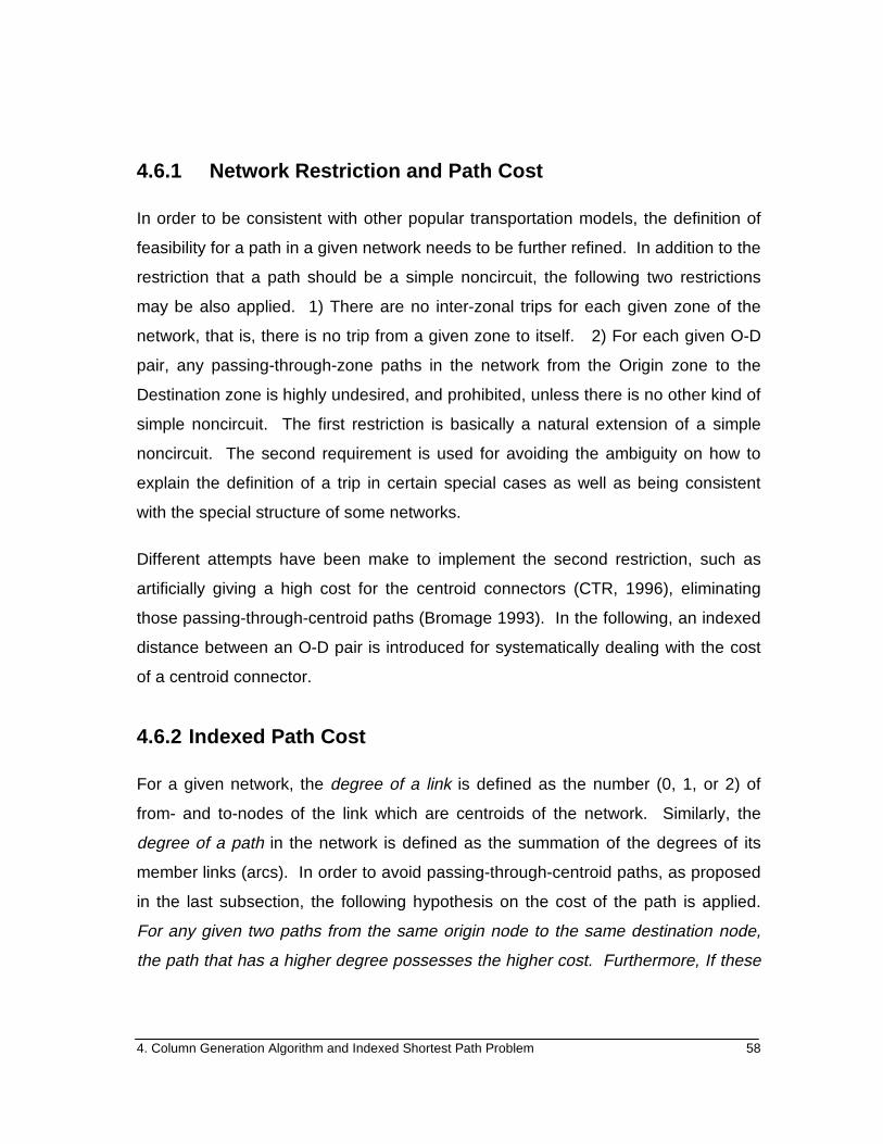
For the same network, if its link costs are indicated via the indexed-cost coefficients,

then the resulting costs will be changed as shown in Figure 4.2.

31 2

5

6

7

8

9

(1,0)

(2,0) (2,0)(2,0)

(1,0)

(1,0)

(1,0)

(1,0)

(1,0)

(1,0)(1,0)(1,0)

(1,0)

(0,1.4)

(0,1.4)4

(2,0)

(1,0)

(0,1.8)

Figure 4.2 . The network of Figure 4.1, using the indexed link cost notation.

Centroid

Intermediate

Given a network, P i i i i i io p p= −{( , ), ( , ), , ( , )}1 1 2 1L and Q j j j jq q= −{( , ), , ( , )}0 1 1L are

two adjacent paths if i jp = 0 . Suppose that their indexed costs are (

c P p p( ) ( , )= 1 2

and (

c Q q q( ) ( , )= 1 2 , respectively. If circuit paths are allowed in the network, then it

can be inductively proved that the followed-up summation of P and Q , denoted as

P Q i i i io

r

+ ={( , ), ( , ),1 1 2 L L, ( , ), ( , ), , ( , )}i i j j j jp p q q− −1 0 1 1 , is a new path with indexed

cost given by

(r

(r(

r

c P Q c P c Q p p q q p q p q( ) ( ) ( ) ( , ) ( , ) ( , ).+ = + = + = + +1 2 1 2 1 1 2 2

Because only simply feasible paths are considered in this research, the above

expression is not correct when a circuit arises in the new resulting path. In this

case, a circuit will be considered as an infeasible path. Therefore, the indexed cost

of the resulting path should be redefined as


++≠≠≠∃≠∞

∞=∞=∞=

=+=+

otherwise.),(

that such , or if)0,(

)0,()(or )0,()( if)0,(

)()()(

2211

00

qpqp

jijjiiji

QcPc

QcPcQPc

lklpkp

((

(v

(v

(

[4.13]

It can be shown that, if infeasible paths (including circuits) are also allowed in the

network, then the set of all paths in the network equipped with the followed-up

summation operation r

+ becomes a semigroup. Moreover, this semigroup is non-

commutative. If there is at least one feasible link in the network, then the subset

consisting of all infeasible paths becomes a proper (double-side) idea of the

semigroup. Obviously, the algebraic property of the derived semigroup depends

only on the structure of the underlying network, and is independent of the definition

of the cost function defined on it.

Finally, in order to implement the hypothesis for ordering relations for the costs

among different paths, define the ordering for the indexed cost as

( , ) ( , ) ( ) )a a b b a b a b a b1 2 1 2 1 1 1 1 2 2> ⇔ > = >or ( and [4.14a]

and

( , ) ( , ) )a a b b a b a b1 2 1 2 1 1 2 2= ⇔ = = ( and . [4.14b]

[4.14a]--[4.14b] define a complete order on the underlying domain.

4.6.3 Shortest Path Problem with Indexed Costs

The shortest path, or minimum cost, problem is one of the most well studied

problems in Operations Research. For a given network G with m nodes, n arcs,

and a cost cij associated with each arc ( , )i j in G , the shortest path problem is to

find the shortest (least costly) path from node 1 to node m in G. The cost of the

path is the sum of the costs on the arcs in the path.


Usually, the cost coefficients of the arcs are real numbers, and the shortest path

problem can be converted into a linear programming problem that automatically

yields {0,1}-values for the decision (arc-choice) variables [Bazaraa, et al., 1990]. In

the case that the costs of the arcs are measured with the indexed cost, this

conversion is still formally true, except that the coefficients of the objective (function)

in the linear program now are denoted with indexed distances. Furthermore, the

most commonly used algorithms for solving the shortest path problem having real

costs can also be slightly modified to solve the shortest path problem with indexed-

cost coefficients. The following examples show how to modify two widely used

algorithms.

A. Dijkstra’s Algorithm with Indexed Costs

This algorithm is a modified version of Dijkstra’s algorithm for the case when all

costs are nonnegative real numbers. The method automatically yields the shortest

path from node 1 to all of the other nodes.

INITIALIZATION STEP

Set ′ =w1 0 0( , ) and let X = { }1 .

MAIN STEP

Let X X= −N , where N is the set of all nodes, and consider the arcs in the

set ( , ) {( , ): , }X X i j i X j X= ∈ ∈ . Let

′ + = ′ +∈

w c w cp pqi j X X

i ij

( (( )

( , ) ( , )

( ){ }1 1Minimum , [4.15]

where (cij( )1 is the indexed link cost from i to j as given by [4.12], and the minimum

is taken according to the relations defined in [4.13a]-[4.13b]. Set ′ = ′ +w w cq p pq

( ( )1 and


place node q in X . Repeat the main step exactly m − 1 times (including the first

time) and then stop; the optimal solution is at hand.

The algorithm above can be validated to produce an optimal solution in the same

manner as for the case of real number costs [Bazaraa et al., 1990], and the detailed

proof is omitted.

As an example, consider the network shown in Figure 4.2. By using the algorithm

above, Figure 4.3 presents a complete solution for this example. The darkened

arcs are those used in the selection of the node to be added to X at each iteration.

They can be used to trace the shortest path from node 1 to any given node i .

31 2

5

6

7

8

9

(1,0)

(2,0) (2,0)(2,0)

(1,0)

(1,0)

(1,0)

(1,0)

(1,0)

(1,0)(1,0)(1,0)(1,0)

(0,1.4)

(0,1.4)4

(2,0)

(1,0)

(0,1.8)

Figure 4.3 . A set of shortest paths using indexed costs.

Centroid

Intermediate

If the network is not rescaled, then Figure 4.4 gives a set of shortest paths

corresponding to the original network (with real costs) from node 1 to all of the other

nodes.


31 2

5

6

7

8

9

1.5

1.3 0.91.3

2.1

1.3

0.8

1.8

3.1

2.21.80.63.8

1.4

1.44

0.4

0.7

1.8

Figure 4.4. A solution of the shortest path problem for the network of Figure 4.1

Centroid

Intermediate

1.2

B. An Algorithm for Determining the Minimum Costs for all Node Pairs

The Dijkstra’s algorithm studied above determines all of the shortest paths from a

given node to all of the other nodes each time. The following algorithm will produce

all of the costs of shortest paths for all possible node pairs.

First, define the 1-step (minimum) cost matrix C cij m m( ) ( )( )1 1= ×

(

, where, for an arbitrary

node pair ( , )i j , the entry (

cij( )1 of the matrix C ( )1 is given by [4.12]. Next, for

r m= −2 1, , ,L define the n -step minimum cost matrix C C Cr r( ) ( ) ( )= •−1 1 . Here, for

two given cost matrices A aij m l= ×( )(

and nlbB ×= )((

, define their “product” matrix

nmijcBAC ×=•= )((

as

njmibac kjiklk

ij ,,1,,,1),(min,,1

LL

(

v((

L

==+==

. [4.16a]

Where, the summation operation “r

+ ” is as defined in 4.13. For each entry (

cijr( ) of

)(rC , if its order is finite, it gives the cost of the shortest path from node i to j

consisting exactly of r links (or traveled in exactly r steps). Finally, for given cost


matrices mmijxX ×= )( and mmijyY ×= )( , define their “summation” matrix

mmijzYXZ ×=⊕= )( as ),min( ijijij yxz = for mji ,,2,1, L= . Let

C c C C C Cijm

minmin ( ) ( ) ( ) ( )( )= = ⊕ ⊕ ⊕ ⊕1 2 3

L , [4.16b]

then, its entries are given by

c c c c i j mij ij ij ijmmin ( ) ( ) ( )min{ , , , }, , , , ,= =−1 2 1 1 2L L [4.16c]

Furthermore, cijmin is the cost of a shortest path from node i to node j .

Remark 4.7 (Indexed costs of infeasible paths) In above algorithms, the indexed

costs for those infeasible links are set to be infinite. In real computer coding,

however, the infinite is usually substituted with a “big number”. Since no circuits are

allowed in the definition of paths, there are at most m − 1 links in a feasible path,

where m is the total number of nodes in the network. Furthermore, the degree for

any given link can be at most 2. Therefore, the number 2m will be used as the

degree for infeasible links or paths.

4.6.4 Linearization and Rescaling Indexed Costs

The indexed cost defined above is highly suitable for the minimum path problem, as

indicated by the algorithm in Section 4.6.3, in addition to satisfying the restrictions

stated in the beginning of Section 4.6.2. On the other hand, from its definition, this

indexed cost function has its range not included in the ordinary real number system.

Moreover, it even does not result in a linear space. Since the major objective used

in this research is based on the linear programming approach, there is a need to

convert these indexed cost functions into real (ranged) functions in the ordinary

sense, in addition to satisfying the restrictions of Section 4.6.2 to a certain extent.

The indexed cost function can be converted into real functions by using the

following linearization method. Suppose that, by using the algorithms described in


last section, the minimum path problem (of indexed type function) has a set of

solutions {( , ), , , , }.(min) (min)d l i jij ij =1 2L Then the cost on a centroid connector of

degree 1 may be defined as

c l i j m i jcentroid ij= + = ≠011

21. max{ , , , , , }(min)L [4.17a]

and the cost of a path from node i to node j , which has indexed-cost ( , )d lij ij , is

given by

c d c lij ij centroid ij= ⋅ + . [4.17b]

If a path ~Pij from node i to node j is a shortest path measured with indexed-cost,

by definition, any other path, say Pij , which also starts from node i and ends to

node j has at least the same degree as ~Pij . If they have the same degree, then

the total cost lij of those non-centroid-connector links in Pij is at least as large as

the total cost ~lij of the non-centroid-connector links in

~Pij . Noting that ccentroid in

[4.17b] is a constant, this implies that the cost of path Pij is not lesser than the cost

of ~Pij even measured with the cost function defined in [4.17]. On the other hand, if

they do not have the same degree, which means that the path Pij passes at least

one more centroid as ~Pij does. Since an extra passing-through-centroid path

increases the degree by at least 2, [4.17] implies that the cost of Pij is larger than

the cost of ~Pij when the cost is defined by [4.17]. That is, a shortest path measured

with indexed cost is also a shortest path measured with the cost given by [4.17].

Similarly, the inverse relation can be proved to be true. This gives the following

lemma.

Lemma 4.3 For any link a A∈ , define the cost function ca on this link by


c

c v a

c

ca

a a

centroid

centroid

=

( ) if is not centroid connector

if one and only one of a’s from - and to - node is a centroid

if both a’s from - and to - node are centroids2

[4.17c]

where c va a( ) is given by [3.3] and ccentroid is defined by [4.17a]. Then the minimum

path problem with the indexed cost function, as described in Sec. 4.6.2, is

equivalent to the minimum path problem with the cost function given by [4.17c], in

the sense that they share the same solution set of paths.

Remark 4.8 (Cost function) In the light of Lemma 4.3 and discussions in Sec. 3.5,

the set of cost functions ca , a A∈ , could be determined in the following steps.

Step1) Use the BPR Equation (4.3) to determine the costs of those non-centroid

connector links on which link volumes are available;

Step2) Assign volumes to those non-centroid connector links with missing volumes

according to the discussion in Chapter 3, and compute the costs on these

links by using the BPR equation;

Step3) Find the minimum path for each O-D pair by using the indexed cost as

discussed in the last section, and determine the cost function ca for each

centroid connector a in terms of [4.17a];

Step4) Finally, the non-penalized cost function cij , for each O-D pair ( , )i j OD∈ , is

given by [4.17b].

4. c generation algorithm and i shortest path problem · simplex method for solving large-sized...

Documents