3D acoustic least-squares reverse time migration using the energy norm

Daniel Rocha1, Paul Sava1, and Antoine Guitton2

ABSTRACT

We have developed a least-squares reverse time migration(LSRTM) method that uses an energy-based imaging condi-tion to obtain faster convergence rates when compared withsimilar methods based on conventional imaging conditions.To achieve our goal, we also define a linearized modelingoperator that is the proper adjoint of the energy migrationoperator. Our modeling and migration operators use spatialand temporal derivatives that attenuate imaging artifacts anddeliver a better representation of the reflectivity and scatteredwavefields. We applied the method to two Gulf of Mexicofield data sets: a 2D towed-streamer benchmark data set anda 3D ocean-bottom node data set. We found LSRTM resolu-tion improvement relative to RTM images, as well as thesuperior convergence rate obtained by the linearized model-ing and migration operators based on the energy norm,coupled with inversion preconditioning using image-domainnonstationary matching filters.

INTRODUCTION

Wavefield migration delivers an image of the subsurface struc-tures using wavefield extrapolation methods (Sun et al., 2003; Bi-ondi, 2012). For complex geologic settings, the two-way waveequation is generally used for extrapolation and the migration pro-cedure is known as reverse time migration (RTM) (Baysal et al.,1983; Lailly, 1983; McMechan, 1983; Levin, 1984; Zhang and Sun,2009). In practice, however, data recording is always incompleteand possibly aliased and irregular, causing wavefield migrationto degrade image quality and resolution especially for greater depths(Zhang et al., 2015). In addition, the obtained image does not fullyexplain data at receiver locations because migration represents theadjoint operator of single-scattering modeling, and, therefore, it is

not a good approximation of the inverse operator that correctlyreverses propagation of seismic data (Claerbout, 1992).Considering these imaging quality issues, least-squares migration

(LSM) is proposed to deliver images with more accurate ampli-tudes, illumination compensation, and reduced footprint of theacquisition geometry (Chavent and Plessix, 1999; Nemeth et al.,1999; Kuehl and Sacchi, 2003; Aoki and Schuster, 2009). If theRTM engine is used for migration, the method is called least-squares RTM (LSRTM) (Dai et al., 2010; Dai and Schuster, 2012;Dong et al., 2012; Yao and Jakubowicz, 2012). LSM involves aforward operator (single-scattering modeling), an adjoint operator(migration), and an objective function, which work together toachieve an image that best explains in a least-squares sense the re-flection data acquired at receivers. The objective function has therole of comparing modeled data with observed data using the imageas reflectivity. To achieve the least-squares solution, we use efficientgradient methods that decrease the objective function iteratively(Hestenes and Stiefel, 1952; Scales, 1987).Because of the high computational cost of LSRTM, which is at

least an order of magnitude higher than RTM, techniques that expediteLSRTM convergence toward the true reflectivity model lead to reduc-tion in computational cost while also achieving a satisfying solution infewer iterations. For instance, a common procedure to obtain fasterrates of convergence is to use an approximate of the Hessian operator(Aoki and Schuster, 2009; Tang, 2009; Dai et al., 2010; Kazemi andSacchi, 2014, 2015; Hou and Symes, 2016; Huang et al., 2016). Here,we demonstrate that modeling and migration operators based on animaging condition that delivers more accurate amplitudes and attenu-ates artifacts, such as the one derived from the energy norm (Doumaet al., 2010; Whitmore and Crawley, 2012; Brandsberg-Dahl et al.,2013; Pestana et al., 2013; Rocha et al., 2016), also expedites con-vergence. This migration operator attenuates low-wavenumber arti-facts, delivering a better representation of subsurface reflectivity.The corresponding modeling operator uses spatial and temporal deriv-atives based on the wave equation itself to generate scattered wave-fields from the energy image. We also incorporate preconditioning

Manuscript received by the Editor 21 July 2017; revised manuscript received 2 December 2017; published ahead of production 14 January 2018; publishedonline 16 March 2018.

1Colorado School of Mines, Center for Wave Phenomena, Golden, Colorado, USA. E-mail: drocha@mines.edu; psava@mines.edu.2DownUnder GeoSolutions, West Perth, Australia and Colorado School of Mines, Center for Wave Phenomena, Golden, Colorado, USA. E-mail: aguitton@

gmail.com.© 2018 Society of Exploration Geophysicists. All rights reserved.

S261

GEOPHYSICS, VOL. 83, NO. 3 (MAY-JUNE 2018); P. S261–S270, 7 FIGS.10.1190/GEO2017-0466.1

Dow

nloa

ded

03/2

1/18

to 1

38.6

7.12

9.87

. Red

istr

ibut

ion

subj

ect t

o SE

G li

cens

e or

cop

yrig

ht; s

ee T

erm

s of

Use

at h

ttp://

libra

ry.s

eg.o

rg/

with an approximation of the Hessian operator in our inversion, whichexpedites LSRTM convergence even more. This approximation of theHessian is achieved by a nonstationary multidimensional filter thatcorrects the blurring effect in the image caused by the wavefield mod-eling and migration operators (Guitton, 2004; Aoki and Schuster,2009; Fletcher et al., 2016).

THEORY

We can define acoustic wavefield migration as an operator suchthat

m0 ¼ LTdobsr ; (1)

where LT is the migration operator based on some imaging condi-tion, dobsr is the single-scattered data observed at receiver locations,and m0 is an image (an estimate of the earth reflectivity). The op-erator LT involves back-propagation of dobsr through an earth model,thus generating a receiver wavefield ur, and the application of animaging condition comparing ur with the source wavefield us. Themigration operator is the adjoint operator of single-scattering mod-eling (or commonly known as linearized modeling). Therefore, L isa linear operator such that

dr ¼ Lm; (2)

and simulates single-scattered data dr at receiver locations using animage containing reflectors that act as sources under the action ofthe source wavefield us.Therefore, we define m as reflectivity that depends on a certain

imaging condition and is not necessarily defined in terms of con-trasts in the earth model. The same principle applies to the linear-ized modeling operator L, which we define as an adjoint operator toa certain imaging condition, and this operator is not directly relatedto the physics of single scattering.

Conventional imaging condition and linearizedmodeling

The conventional imaging condition is defined as the zero-lagcrosscorrelation between source and receiver wavefields us and ur:

m0 ¼ uTs ur: (3)

Because we know both wavefields are generated by extrapolationusing an earth model and observed data at receivers, we can rewriteequation 3 as

m0 ¼ ðEþKsdsÞTE−Krdobsr ; (4)

where Eþ and E− are the forward and backward extrapolator oper-ators, Ks and Kr are the source and receiver injection operators (seeAppendix A), respectively, and ds is the source function. The sub-scripts in the extrapolator operators indicate extrapolation directionfor either positive (þ) or negative (−) times. Note the two importantrelations between the extrapolator operators: Eþ ¼ ET

− andE− ¼ ETþ. Then, one can write equation 4 similarly to equation 1:

m0 ¼ LTdobsr ; (5)

where

LT ¼ ðEþKsdsÞTE−Kr: (6)

We can obtain the operator L (adjoint of LT) if we apply the adjointfor each individual operator and reverse the order of operators.Therefore, conventional linearized modeling is defined as

dr ¼ Lm; (7)

where

L ¼ KTrEþðEþKsdsÞ ¼ KT

rEþus: (8)

In other words, single-scattered data dr are obtained by extraction atthe receiver locations (KT

r ), and wavefield extrapolation (Eþ) usingusm as the source term.

Energy imaging condition and linearized modeling

For an extrapolated wavefield that satisfies the acoustic-waveequation, we can compute its energy norm in discretized spaceand time as (Rocha et al., 2016)

kuk2E ¼Xx;t

�_u2

v2ðxÞ þ j∇uj2�; (9)

where vðxÞ is the migration velocity, superscript dot indicates thetime differentiation, and ∇ is the spatial gradient. On the right sideof equation 9, the first term inside the brackets corresponds to thekinetic energy of the wavefield, and the second term corresponds toits potential energy. Based on this norm, we can define an imagingcondition that ignores wave events between source and receiver wave-fields that share the same propagation direction, thus suppressinglow-wavenumber artifacts in RTM that do not characterize subsurfacereflectivity:

m0ðxÞ ¼Xt

�_us _urv2

− ∇us · ∇ur�: (10)

A more compact form of equation 10 uses the energy operator

□ ¼�∇;

1

vðxÞ∂∂t

�; (11)

which computes a 4D vector field from the scalar wavefield. A neg-ative time derivative is implied for the back-propagated receiver wave-field ur. If we compute the dot product between such vector fieldsobtained from source and receiver wavefields at each spatial location(implying summation over time), we can rewrite equation 10 as

m0 ¼ ð□usÞT□ur: (12)

Using the operators introduced in equations 4 and 12 becomes

m0 ¼ ð□EþKsdsÞT□E−Krdobsr : (13)

Because equation 13 is a function of dr, we can write the correspond-ing migration operation as

m0 ¼ LTdobsr ; (14)

S262 Rocha et al.

Dow

nloa

ded

03/2

1/18

to 1

38.6

7.12

9.87

. Red

istr

ibut

ion

subj

ect t

o SE

G li

cens

e or

cop

yrig

ht; s

ee T

erm

s of

Use

at h

ttp://

libra

ry.s

eg.o

rg/

where

LT ¼ ð□EþKsdsÞT□E−Kr: (15)

Therefore, the linearized modeling operation based on the energynorm is defined as

dr ¼ Lm; (16)

where

L ¼ KTrEþ□T□ðEþKsdsÞ ¼ KT

rEþ□T□us: (17)

In other words, single-scattered data dr are obtained by extraction atthe receiver locations (KT

r ), and wavefield extrapolation (Eþ) with□T□usm as the source term, which for a point in space and timecan explicitly be written as

½□T□usm�ðx;tÞ¼mðxÞv2ðxÞusðx;tÞ−∇ · ½mðxÞ∇usðx;tÞ�. (18)

The same procedure to find a proper adjoint operator is applicableto other imaging conditions. For instance, applying a Laplacianoperator on a conventional image is theoretically equivalent to theapplication of the energy imaging condition but in the far field(Douma et al., 2010). Knowing that the Laplacian operator is self-adjoint, the imaging condition with Laplacian filtering can be writtenas

m0 ¼ ∇2uTs ur: (19)

The corresponding linearized modeling is written as

dr ¼ Lm; (20)

where

L ¼ KTrEþðEþKsdsÞ∇2 ¼ KT

rEþus∇2: (21)

The source term for this case is us∇2m and can explicitly be writtenfor each point in space and time as

½us∇2m�ðx; tÞ ¼ usðx; tÞ∇2m: (22)

LSM and preconditioning with an approximation ofthe Hessian

A pair of linearized modeling and migration operators enables usto compute an image that minimizes the L2 norm of the differencebetween observed and modeled data:

EðmÞ ¼ 1

2kLm − dobsr k2; (23)

and such image is mathematically described by

mLS ¼ ðLTLÞ−1LTdobsr : (24)

To findmLS, one generally uses iterative procedures that exploit thedirection of the gradient of the objective function in equation 23 at agiven iteration i:

gi ¼∂EðmiÞ∂mi

¼ LTðLmi − dobsr Þ; (25)

and the model update at each iteration in steepest descent and con-jugate gradient methods is a scaled version of the gradient

miþ1 ¼ mi − αgi: (26)

In equation 24, the term LTL is known as the Hessian operator ofEðmÞ. If the inverse of the Hessian is applied to the RTM imageLTdobsr , the least-squares solution is achieved. However, in practice,the Hessian operator cannot explicitly be computed for LSM prob-lems. As suggested by Guitton (2004), we can obtain an approxi-mation of the Hessian operator if we compute an image

m1 ¼ LTLm0; (27)

wherem0 ¼ LTdobsr is the standard RTM image. The operator B thatminimizes

EðBÞ ¼ km0 − Bm1k2; (28)

is a good approximation of the inverse of the Hessian ðLTLÞ−1 ac-cording to equation 27. Here, we define the operator B as a multi-dimensional convolutional operator along all spatial axes (Rickettet al., 2001).Once we obtain the approximation of the inverse of the Hessian,

we can expedite convergence in least-squares inversion by precon-ditioning the gradient with the operator B before updating the modelat each iteration. Incorporating the preconditioning, equation 26becomes

miþ1 ¼ mi − αBgi: (29)

EXAMPLES

To show how LSRTM with proper imaging operators can getfaster convergence rates relative to conventional methods, we per-form an LSRTM experiment using a 2D Gulf of Mexico (GOM)data set, used by many authors in the past as a benchmark data set(Dragoset, 1999; Guitton and Cambois, 1999; Hadidi et al., 1999;Lamont et al., 1999; Lokshtanov, 1999; Verschuur and Prein, 1999)and described by Guitton et al. (2012). Such a 2D data set is usefulto test the capability of the energy imaging operators in attenuatinglow-wavenumber artifacts caused by strong velocity contrasts (suchas a salt body) and to benchmark our inversion procedure beforeapplication to a larger 3D data set. Standard preprocessing is appliedto the data set prior to LSRTM, such as surface-related multiplesuppression. We use 71 of the original 1001 shot records, withthe first source location at x ¼ 4000 m and the last at x ¼ 22;670 m,resulting in a source spacing of approximately 267 m. The shot deci-mation decreases the computational cost of the entire experiment andalso introduces truncation artifacts, which are useful to test the effec-tiveness of our LSRTM in attenuating acquisition artifacts. Each shotrecord contains 180 traces with receiver spacing of 26.67 m and amaximum offset of 4874 m. For migration, we use a maximum fre-quency of 40 Hz and a spatial sampling of 6.67 m. A standard RTMmigration (Figure 1a) exhibits low-wavenumber artifacts and poorillumination in the subsalt area. We test two alternative LSRTMs,one using modeling and migration with the Laplacian operator

3D acoustic LSRTM with the energy norm S263

Dow

nloa

ded

03/2

1/18

to 1

38.6

7.12

9.87

. Red

istr

ibut

ion

subj

ect t

o SE

G li

cens

e or

cop

yrig

ht; s

ee T

erm

s of

Use

at h

ttp://

libra

ry.s

eg.o

rg/

(equations 19 and 21), and the other based on the energy norm (equa-tions 15 and 17). For this experiment, the final images from theLaplacian and energy LSRTMs are similar in quality and resolution,and we show the final energy LSRTM image in Figure 1b, whichcontains suppressed low-wavenumber artifacts above the salt bodyas compared with the conventional image in Figure 1a. In addition,the objective functions (Figure 1c) of both alternative LSRTMs de-crease faster than the one from conventional LSRTM, with the onebased on the energy norm decreasing slightly faster when comparedwith its Laplacian counterpart. Although the two alternative LSRTMimplementations are theoretically equivalent far from the source and

receiver locations, one computes the imaging condition in the imagedomain and the other in the wavefield domain, leading to slightlydifferent numerical implementations and, therefore, convergenceperformances. The energy migration and modeling operators appliedeither in the wavefield domain (equation 18) or in the image domainas a Laplacian operator provide faster convergence rates toward thefinal reflectivity model.We apply our method to a 3D ocean-bottom node data set from

the GOM. We process the data set to obtain only the downgoingpressure component and perform mirror imaging (Godfrey et al.,1998; Ronen et al., 2005; Wong et al., 2010, 2015) of shallow geo-logic structures with a fine spatial sampling of 12.5 m. We use 37node gathers with sources densely distributed at the water surface(Figure 2a), and the velocity model used is shown in Figure 2b. Intotal, as shown in Figure 2c, we perform four LSRTM experiments:

a)

b)

c)

Figure 1. The GOM 2D data set: (a) conventional RTM image and(b) LSRTM imagewith the energymodeling and migration operators.(c) Normalized objective functions for conventional LSRTM (blue),LSRTM with Laplacian (red) and based on the energy norm (green).Note suppression of low-wavenumber artifacts above the salt and theconvergence speed-up obtained by the alternative LSRTMs.

y

a)

b)

c)

Figure 2. The GOM 3D data set: (a) 37 nodes spaced by approxi-mately 800 m and sources densely distributed at the surface of themodel. (b) Velocity model. (c) Normalized objective functions forconventional (blue), Laplacian-based (red), energy-based (green), andpreconditioned energy-based (black and then green at iteration 2)LSRTMs. The energy LSRTM has the best performance if we applypreconditioning at the first two iterations.

S264 Rocha et al.

Dow

nloa

ded

03/2

1/18

to 1

38.6

7.12

9.87

. Red

istr

ibut

ion

subj

ect t

o SE

G li

cens

e or

cop

yrig

ht; s

ee T

erm

s of

Use

at h

ttp://

libra

ry.s

eg.o

rg/

a)b)

c)d)

e) f)

Figure 3. The GOM 3D data set: depth slices at z ¼ 1.55 km and z ¼ 1.77 km, respectively, for (a/b) RTM, (c/d) conventional LSRTM, and(e/f) energy LSRTMwith preconditioning. In the LSRTM images, note the improvement in focusing of the diffractors and in delineation of thereflectors.

3D acoustic LSRTM with the energy norm S265

Dow

nloa

ded

03/2

1/18

to 1

38.6

7.12

9.87

. Red

istr

ibut

ion

subj

ect t

o SE

G li

cens

e or

cop

yrig

ht; s

ee T

erm

s of

Use

at h

ttp://

libra

ry.s

eg.o

rg/

conventional LSRTM, Laplacian-based LSRTM, and energy-normbased LSRTMwith and without preconditioning. Similar to the pre-ceding example, conventional LSRTM has a worse performance in

terms of objective function decrease, and the energy LSRTM has aslightly smaller objective function value over iterations comparedwith its Laplacian counterpart. We compute the matching filter

for the preconditioning using the energy RTMimage (m0 ¼ LTdobsr ) and an image generated bym1 ¼ LTLm0, where the modeling (L) and mi-gration (LT) operators are based on the energynorm. We use the preconditioning at the two firstiterations and switch it off at the second iteration(solid black and green lines in Figure 2c) becausethe computed matching filter is related to the im-ages at the first and second iterations (m0 andm1).The matching filter is biased toward the strongamplitude changes between such images at firstiterations, and keeping preconditioning on doesnot give substantial benefit to the inversion at lateriterations, thus only increasing computationalcost. Although we apply the preconditioning only

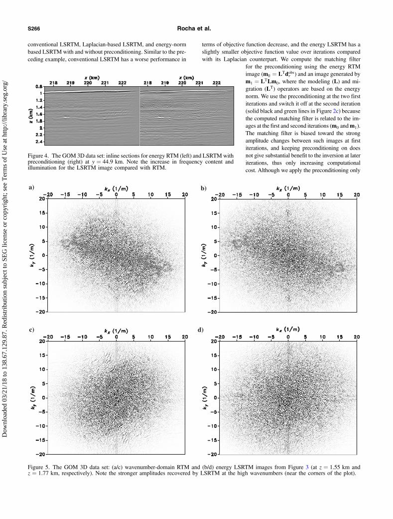
Figure 4. The GOM 3D data set: inline sections for energy RTM (left) and LSRTMwithpreconditioning (right) at y ¼ 44.9 km. Note the increase in frequency content andillumination for the LSRTM image compared with RTM.

a) b)

c) d)

Figure 5. The GOM 3D data set: (a/c) wavenumber-domain RTM and (b/d) energy LSRTM images from Figure 3 (at z ¼ 1.55 km andz ¼ 1.77 km, respectively). Note the stronger amplitudes recovered by LSRTM at the high wavenumbers (near the corners of the plot).

S266 Rocha et al.

Dow

nloa

ded

03/2

1/18

to 1

38.6

7.12

9.87

. Red

istr

ibut

ion

subj

ect t

o SE

G li

cens

e or

cop

yrig

ht; s

ee T

erm

s of

Use

at h

ttp://

libra

ry.s

eg.o

rg/

at the first iterations, we obtain a significant speed-up in the conver-gence rate over all subsequent iterations.For two different areas of the migration volume, the depth slices

in Figure 3 compare RTM, conventional LSRTM, and our LSRTMthat uses energy imaging operators and preconditioning. Althoughconventional LSRTM fits less data and has the worst convergencerate based on Figure 2c, it delivers images closer in quality to ourLSRTM images (Figure 3e and 3f). In these depth slices, some im-aged events that seem to disappear or become blurry after LSRTMmight indicate that they do not correctly predict reflection events inthe data domain, considering that our imaging operator is isotropicand acoustic. Figure 4 compares RTM and our LSRTM cross-sec-tional images side by side and shows the visual benefit due to theincrease in illumination and frequency contents (especially towardthe low frequencies) in the LSRTM image. To confirm the increasein bandwidth for the depth slices, we transform the images fromFigure 3 to the wavenumber domain and obtain the spectral imagesin Figure 5. Note how LSRTM recovers high-resolution content byspreading the amplitudes toward the edges of the wavenumber do-main. However, one needs to consider that some recovered high-wavenumber content might emerge from noise existent in the data.As discussed in the “Theory” section, one of the benefits in

LSRTM is to suppress the acquisition footprint. In some shallowareas of the migration volume, very close to the edges of the modeland to the water bottom, imaging artifacts exist in the RTM imagedue to the large decimation of nodes for this experiment (from 924to 37 nodes, causing nodes to be quite sparse as seen in Figure 2a)and the irregularity of source and receiver locations with respect tothe regular extrapolation grid. Figure 6 shows an example: LSRTM(Figure 6b) attenuates some of these acquisition footprint artifacts atthe water bottom from the RTM image (Figure 6a). Figure 7 com-pares observed and predicted data at the last iteration, and the dif-ference (residual) between the two for a gather of traces sortedby increasing offset at a particular node location (x ¼ 214.5 km,y ¼ 44.9 km). Note that the main reflections at near and mid offsetsare correctly predicted, but the far-offset amplitudes are not matchedmainly because of elasticity and anisotropy, which are not accountedfor by our acoustic imaging operators. As expected, the residual inFigure 7c still exhibits noise, such as a large dipping event that goesfrom t ¼ 2.2s at trace 0 to t ¼ 3.0s at trace 10,000. In summary, withseveral iterations corresponding to an order of magnitude of the stan-dard RTM computational cost, we obtain LSRTM images that exhibitmore focused diffractions and delineated structures, as shown by thedepth slices in Figure 3.

DISCUSSION

The main advantage of our method when compared with conven-tional LSRTM is accelerated convergence to an optimal solution, asshown in Figures 1c and 2c. The energy imaging better recovers thereflector amplitudes and scattered wavefields, resulting in a closermatch between the observed and simulated data. Second-order fac-tors accountable for the decrease of the objective function includethe mitigation of imaging artifacts and sharper focusing of events,and both of these improvements are similar between the energy(Figure 3e and 3f) and conventional (Figure 3c and 3d) LSRTMimages.In terms of computational cost, the energy LSRTM does not add

significant burden. During extrapolation of source and receiverwavefields, the same finite-difference differential operators applied

at each time step of wave extrapolation can also be applied to com-pute the terms required for the image (equation 10) or for the lin-earized source term (equation 18). In case these operators cannot beefficiently applied to the wavefields (e.g., insufficient memory stor-age for additional wavefield variables), the Laplacian-based imag-ing operators, although only adequate for image regions away fromsource and receiver locations, serve as good substitutes as seen bythe convergence plots in Figures 1c and 2c.We empirically observe that the preconditioning based on the

matching filters benefits the first two iterations only (Figure 2c). Thiseffect can be explained analytically by the fact that the least-squaressolution of the filter estimation problem is

B ¼ ðMT1M1Þ−1MT

1M0; (30)

where

M1 ¼ LTLM0 (31)

is the nonstationary convolutional operator using the entries of m1.Similarly, M0 is the corresponding convolutional operator for m0.Substituting equation 31 into equation 30 yields

a)

b)

Figure 6. The GOM 3D data set: depth slices for (a) RTM and(b) LSRTM at the water bottom (z ¼ 1.20 km). Note the artifactsuppression in some locations indicated by the white circles.

3D acoustic LSRTM with the energy norm S267

Dow

nloa

ded

03/2

1/18

to 1

38.6

7.12

9.87

. Red

istr

ibut

ion

subj

ect t

o SE

G li

cens

e or

cop

yrig

ht; s

ee T

erm

s of

Use

at h

ttp://

libra

ry.s

eg.o

rg/

B ¼ ðMT0L

TLLTLM0Þ−1MT0L

TLM0; (32)

which shows that the filters can be seen as a least-squares estimate ofthe inverse Hessian operator ðLTLÞ−1, left and right multiplied by the

convolutional operator M0. There is, therefore, an influence of thestarting image m0 to the approximate inverse Hessian. In effect, thematching filters are a very good approximation of the operator takingus between the vectors m0 andm1 of the Krylov subspace generatedby LTL only (and used in the first two iterations of the conjugategradient method). Beyond these two iterations, the matching filtersdo not provide any benefit anymore and switching to a nonprecondi-tioned inversion proves the most effective strategy (as illustrated inFigure 2c). Guitton (2017) also exemplifies this point on 3D syntheticand field data cases. As possible improvements, but not tested here,one could reestimate the matching filters as the iterations go on or finddifferent reference images m0 and m1 for the filter estimation step.Alternatively, our LSRTM preconditioning with matching filters

can be implemented using point-spread functions (PSFs) (Fletcheret al., 2016). In our case, this approach involves creating a referenceimagem0 with spikes regularly spaced and then computing m1 afterlinearized modeling and migration of the reference image with spikes(m0). However, spike spacing parameterization involves an inherenttrade-off between fine and coarse sampling. Too much fine samplingcauses an overlap of the blurred events, thus undermining our abilityto accurately extract the PSFs, and too much coarse sampling doesnot capture enough of the subsurface structure details. In addition,this approach requires a robust interpolation of the matching filter forimage samples away from the spikes. Therefore, we do not use thisalternative approach for the computation of the matching filters.

CONCLUSION

We demonstrate that using proper linearized modeling and migra-tion operators expedites LSRTM, which otherwise suffers fromhigh computational cost. We test modeling and migration operatorsbased on the energy norm, and we obtain faster convergence ratesfor LSRTM inversion because the energy operators attenuate arti-facts that do not properly characterize subsurface reflectivity. Inaddition, a preconditioning operator that uses a multidimensionalnonstationary matching filter decreases the objective function sub-stantially at the first iterations, allowing a significant speed-up forthe following iterations. Our field data examples show significantimage quality improvement within less than 10 inversion iterationsusing an accelerated LSRTM compared with regular RTM.

ACKNOWLEDGMENTS

We thank the sponsors of the Center for Wave Phenomena, whosesupport made this research possible. We are grateful to the ShellExploration and Production Company for sharing the 3D GOM dataset with Colorado School of Mines and their permission to publishthe results using this data set. The authors appreciate the constructivecomments from the anonymous reviewers of this paper. The repro-ducible numeric examples in this paper use the Madagascar open-source software package (Fomel et al., 2013) available at http://www.ahay.org.

APPENDIX A

CONVENTIONAL MIGRATION AND MODELINGOPERATORS

For source and receiver wavefields usðx; tÞ and urðx; tÞ, an imagem0ðxÞ is conventionally obtained by

a)

b)

c)

d)

Figure 7. The GOM 3D data set: node gather at x ¼ 214.5 km andy ¼ 44.9 km sorted by increasing offset: (a) observed, final (b) pre-dicted and (c) residual data. (d) Offset values for each trace. Notethat the main reflection events are predicted and eliminated in thedata residual, especially for events at near- and mid-offsets. Linearmoveout is applied on these plots for display purposes.

S268 Rocha et al.

Dow

nloa

ded

03/2

1/18

to 1

38.6

7.12

9.87

. Red

istr

ibut

ion

subj

ect t

o SE

G li

cens

e or

cop

yrig

ht; s

ee T

erm

s of

Use

at h

ttp://

libra

ry.s

eg.o

rg/

m0 ¼ uTs ur: (A-1)

We can represent equation A-1 and the following equations pic-torially using matrices, which indicate the relative dimensions ofoperators and variables:

By using forward and backward extrapolator operators Eþðx; tÞand E−ðx; tÞ, and source and receiver injection operatorsKsðx; xs; tÞ and Krðx; xr; tÞ, we have

m0 ¼ ðEþKsdsÞTE−Krdobsr ; (A-2)

where dsðxs; tÞ and dobsr ðxr; tÞ are the source and receiver data, re-spectively. In compact form, we can rewrite equation A-2 as

m0 ¼ LTdobsr : (A-3)

Linearized modeling is defined as

dr ¼ Lm: (A-4)

Based on equations A-2 and A-3, we can rewrite equation A-4 as

dr ¼ KTrET

−usm; (A-5)

or

dr ¼ KTrEþðEþKsdsÞm; (A-6)

where ET− ¼ Eþ, and KT

r represents the extraction at the receiverlocations (adjoint operator of the injection operator).

APPENDIX B

ENERGY MIGRATION AND MODELINGOPERATORS

The energy image m0ðxÞ is obtained by

m0 ¼ ð□usÞT□ur: (B-1)

The operator □ turns an acoustic wavefield into a vector field ofwhich components are spatial and temporal. We represent this in-crease in dimensions pictorially by making the matrix of □ consid-erably larger than the wavefields matrices. Using extrapolator andinjection operators, we have

m0 ¼ ð□EþKsdsÞT□E−Krdobsr : (B-2)

In compact form, we can rewrite equation B-2 as

m0 ¼ LTdobsr : (B-3)

Linearized modeling is defined as

dr ¼ Lm: (B-4)

Based on equations B-2 and B-3, we can rewrite equation B-4as

dr ¼ KTrET

−□T□usm; (B-5)

3D acoustic LSRTM with the energy norm S269

Dow

nloa

ded

03/2

1/18

to 1

38.6

7.12

9.87

. Red

istr

ibut

ion

subj

ect t

o SE

G li

cens

e or

cop

yrig

ht; s

ee T

erm

s of

Use

at h

ttp://

libra

ry.s

eg.o

rg/

or

dr ¼ KTrEþ□T□ðEþKsdsÞm: (B-6)

REFERENCES

Aoki, N., and G. T. Schuster, 2009, Fast least-squares migration with a de-blurring filter: Geophysics, 74, no. 6, WCA83–WCA93, doi: 10.1190/1.3155162.

Baysal, E., D. D. Kosloff, and J. W. C. Sherwood, 1983, Reverse time mi-gration: Geophysics, 48, 1514–1524, doi: 10.1190/1.1441434.

Biondi, B., 2012, 3D seismic imaging: SEG.Brandsberg-Dahl, S., N. Chemingui, D. Whitmore, S. Crawley, E. Klochi-

khina, and A. Valenciano, 2013, 3D RTM angle gathers using an inversescattering imaging condition: 83rd Annual International Meeting, SEG,Expanded Abstracts, 3958–3962.

Chavent, G., and R.-E. Plessix, 1999, An optimal true-amplitude least-squaresprestack depth-migration operator: Geophysics, 64, 508–515, doi: 10.1190/1.1444557.

Claerbout, J. F., 1992, Earth soundings analysis: Processing versus inver-sion: Blackwell Scientific Publications.

Dai, W., C. Boonyasiriwat, and G. Schuster, 2010, 3D multisource least-squares reverse-time migration: 80th Annual International Meeting, SEG,Expanded Abstracts, 3120–3124.

Dai, W., and G. T. Schuster, 2012, Plane-wave least-squares reverse time mi-gration: 82nd Annual International Meeting, SEG, Expanded Abstracts,doi: 10.1190/segam2012-0382.1.

Dong, S., J. Cai, M. Guo, S. Suh, Z. Zhang, B. Wang, and Z. Li, 2012, Least-squares reverse time migration: Towards true amplitude imaging and im-proving the resolution: 82nd Annual International Meeting, SEG, ExpandedAbstracts, doi: 10.1190/segam2012-1488.1.

Douma, H., D. Yingst, I. Vasconcelos, and J. Tromp, 2010, On the connec-tion between artifact filtering in reverse-time migration and adjointtomography: Geophysics, 75, no. 6, S219–S223, doi: 10.1190/1.3505124.

Dragoset, B., 1999, A practical approach to surface multiple attenuation:The Leading Edge, 18, 104–108, doi: 10.1190/1.1438132.

Fletcher, R. P., D. Nichols, R. Bloor, and R. T. Coates, 2016, Least-squaresmigration: Data domain versus image domain using point spread func-tions: The Leading Edge, 35, 157–162, doi: 10.1190/tle35020157.1.

Fomel, S., P. Sava, I. Vlad, Y. Liu, and V. Bashkardin, 2013, Madagascar:Open-source software project for multidimensional data analysis and repro-ducible computational experiments: Journal of Open Research Software, 1,e8, doi: 10.5334/jors.ag.

Godfrey, R., P. Kristiansen, B. Armstrong,M. Copper, and E. Thorogood, 1998,Imaging the Foinaven ghost: 68th Annual International Meeting, SEG, Ex-panded Abstracts, 1333–1335.

Guitton, A., 2004, Amplitude and kinematic corrections of migrated imagesfor nonunitary imaging operators: Geophysics, 69, 1017–1024, doi: 10.1190/1.1778244.

Guitton, A., 2017, Fast 3D least-squares RTM by preconditioning withnon-stationary matching filters: 87th Annual International Meeting,SEG, Expanded Abstracts, 4395–4399.

Guitton, A., G. Ayeni, and E. Daz, 2012, Constrained full-waveform inver-sion by model reparameterization: Geophysics, 77, no. 2, R117–R127,doi: 10.1190/geo2011-0196.1.

Guitton, A., and G. Cambois, 1999, Multiple elimination using a pattern-rec-ognition technique: The Leading Edge, 18, 92–98, doi: 10.1190/1.1438166.

Hadidi, M. T., M. Sabih, D. E. Johnston, and C. Calderon-Macias, 1999,Mobil’s results for the 1997 workshop on multiple attenuation: The Lead-ing Edge, 18, 100–103, doi: 10.1190/1.1513313.

Hestenes, M. R., and E. Stiefel, 1952, Methods of conjugate gradients forsolving linear systems: Journal of Research of the National Bureau ofStandards, 49, 409–436, doi: 10.6028/jres.049.044.

Hou, J., and W. W. Symes, 2016, Accelerating extended least-squares mi-gration with weighted conjugate gradient iteration: Geophysics, 81, no. 4,S165–S179, doi: 10.1190/geo2015-0499.1.

Huang, W., P. Deng, and H.-W. Zhou, 2016, Least-squares reverse-time mi-gration with hessian preconditioning: 86th Annual International Meeting,SEG, Expanded Abstracts, 1043–1046.

Kazemi, N., and M. Sacchi, 2014, Filter-based least squares wave equationshot profile migration: 76th Annual International Conference and Exhi-bition, EAGE, Extended Abstracts, doi: 10.3997/2214-4609.20141225.

Kazemi, N., and M. D. Sacchi, 2015, Block row recursive least-squares mi-gration: Geophysics, 80, no. 5, A95–A101, doi: 10.1190/geo2015-0070.1.

Kuehl, H., and M. D. Sacchi, 2003, Least-squares wave-equation migrationfor AVO/AVA inversion: Geophysics, 68, 262–273, doi: 10.1190/1.1543212.

Lailly, P., 1983, The seismic inverse problem as a sequence of before stackmigrations: Proceedings of the Conference on Inverse Scattering, Theoryand Application, SIAM, 206–220.

Lamont, M. G., B. M. Hartley, and N. F. Uren, 1999, Multiple attenuationusing the MMO and ISR preconditioning transforms: The Leading Edge,18, 110–114, doi: 10.1190/1.1438134.

Levin, S. A., 1984, Principle of reverse-time migration: Geophysics, 49,581–583, doi: 10.1190/1.1441693.

Lokshtanov, D., 1999, Multiple suppression by data-consistent deconvolu-tion: The Leading Edge, 18, 115–119, doi: 10.1190/1.1438136.

McMechan, G. A., 1983, Migration by extrapolation of time dependentboundary values: Geophysical Prospecting, 31, 413–420, doi: 10.1111/j.1365-2478.1983.tb01060.x.

Nemeth, T., C. Wu, and G. T. Schuster, 1999, Least-squares migration of in-complete reflection data: Geophysics, 64, 208–221, doi: 10.1190/1.1444517.

Pestana, R., A. W. G. dos Santos, and E. S. Araujo, 2013, RTM imaging con-dition using impedance sensitivity kernel combined with Poynting vector:Proceedings of the 13th International Congress of The Brazilian Geophysi-cal Society.

Rickett, J., A. Guitton, and D. Gratwick, 2001, Adaptive multiple subtrac-tion with non-stationary helical shaping filters: 63rd Annual InternationalConference and Exhibition, EAGE, Extended Abstracts, P167.

Rocha, D., N. Tanushev, and P. Sava, 2016, Acoustic wavefield imaging usingthe energy norm: Geophysics, 81, no. 4, S151–S163, doi: 10.1190/geo2015-0486.1.

Ronen, S., L. Comeaux, and X.-G. Miao, 2005, Imaging downgoing wavesfrom ocean bottom stations: 75th Annual International Meeting, SEG, Ex-panded Abstracts, 963–967.

Scales, J., 1987, Tomographic inversion via the conjugate gradient method:Geophysics, 52, 179–185, doi: 10.1190/1.1442293.

Sun, J., Y. Zhang, S. Gray, C. Notfors, and J. Young, 2003, 3-D prestackdepth migration by wave-field extrapolation methods: 16th GeophysicalConference, ASEG, Extended Abstracts, 1–4.

Tang, Y., 2009, Target-oriented wave-equation least-squares migration/in-version with phase-encoded Hessian: Geophysics, 74, no. 6, WCA95–WCA107, doi: 10.1190/1.3204768.

Verschuur, D. J., and R. J. Prein, 1999, Multiple removal results from DelftUniversity: The Leading Edge, 18, 86–91, doi: 10.1190/1.1438164.

Whitmore, N. D., and S. Crawley, 2012, Application of RTM inverse scat-tering imaging conditions: 82nd Annual International Meeting, SEG, Ex-panded Abstracts, doi: 10.1190/segam2012-0779.1.

Wong, M., B. L. Biondi, and S. Ronen, 2010, Joint least-squares inversion ofup- and down-going signal for ocean bottom data sets: 80th Annual Inter-national Meeting, SEG, Expanded Abstracts, 2752–2756.

Wong, M., B. L. Biondi, and S. Ronen, 2015, Imaging with primaries andfree-surface multiples by joint least-squares reverse time migration: Geo-physics, 80, no. 6, S223–S235, doi: 10.1190/geo2015-0093.1.

Yao, G., and H. Jakubowicz, 2012, Least-squares reverse-time migration:82nd Annual International Meeting, SEG, Expanded Abstracts, doi: 10.1190/segam2012-1425.1.

Zhang, Y., L. Duan, and Y. Xie, 2015, A stable and practical implementationof least-squares reverse time migration: Geophysics, 80, no. 1, V23–V31,doi: 10.1190/geo2013-0461.1.

Zhang, Y., and J. Sun, 2009, Practical issues in reverse time migration: Trueamplitude gathers, noise removal and harmonic source encoding: FirstBreak, 27, 53–59, doi: 10.3997/1365-2397.2009002.

S270 Rocha et al.

Dow

nloa

ded

03/2

1/18

to 1

38.6

7.12

9.87

. Red

istr

ibut

ion

subj

ect t

o SE

G li

cens

e or

cop

yrig

ht; s

ee T

erm

s of

Use

at h

ttp://

libra

ry.s

eg.o

rg/