It's Not Factor Accumulation: Stylized Facts and Growth Models

William Easterly and Ross Levine

March 2001

Abstract: We document five stylized facts of economic growth. (1) The “residual” rather than factor accumulation accounts for most of the income and growth differences across nations. (2) Income diverges over the long run. (3) Factor accumulation is persistent while growth is not persistent and the growth path of countries exhibits remarkable variation across countries. (4) Economic activity is highly concentrated, with all factors of production flowing to the richest areas. (5) National policies closely associated with long-run economic growth rates. We argue that these facts do not support models with diminishing returns, constant returns to scale, some fixed factor of production, and that highlight the role of factor accumulation. Empirical work, however, does not yet decisively distinguish among the different theoretical conceptions of “total factor productivity growth.” Economists should devote more effort towards modeling and quantifying total factor productivity. *Easterly: Development Research Group, World Bank (WEasterly@WorldBank.Org); Levine: University of Minnesota (Rlevine@csom.umn.edu). We owe a great deal to Lant Pritchett, who shaped the paper, gave comments, and provided many of the “stylized facts.” We are grateful to François Bourguignon, Ashok Dhareshwar, Robert G. King, Michael Kremer, Peter Klenow, Paul Romer, Xavier Sala-i-Martin, Robert Solow, Albert Zeufack, two anonymous referees, and to students and faculty at the Economics Education Research Consortium program in Kiev, Ukraine, Harvard Kennedy School, and Johns Hopkins-SAIS, and to participants in the February 2001 World Bank conference "What have we learned from a decade of empirical research on growth?" for useful comments. This paper’s findings, interpretations, and conclusions are entirely those of the authors and do not necessarily represent the views of the World Bank, its Executive Directors, or the countries they represent.

1

The central problem in understanding economic development and growth is not to understand the

process by which an economy raises its savings rate and increases the rate of physical capital accumulation.1

Although many development practitioners and researchers continue to target capital accumulation as the

driving force in economic growth,2 this paper presents evidence regarding the sources of economic growth, the

patterns of economic growth, the patterns of factor flows, and the impact of national policies on economic

growth that suggest that “something else” besides capital accumulation is critical for understanding differences

in economic growth and income across countries. The paper does not argue that factor accumulation is

unimportant in general, nor do we deny that factor accumulation is critically important for some countries at

specific junctures. The paper’s more limited point is that when comparing growth experiences across many

countries, “something else” – besides factor accumulation – plays a prominent role in explaining differences in

economic performance. As Robert Solow argued in 1956, economists construct models to reproduce crucial

empirical regularities and then use these models to interpret economic events and make policy

recommendations. This paper documents important empirical regularities regarding economic growth in the

hopes of highlighting productive directions for future research and improving public policy.

A growing body of research suggests that after accounting for physical and human capital

accumulation, “something else” accounts for the bulk of cross-country growth differences. This “something

else” accounts for the majority of cross-country differences in both the level of Gross Domestic Product (GDP)

per capita and the growth rate of GDP per capita. The profession typically uses the term “Total Factor

Productivity (TFP)” to refer to the “something else” (besides physical factor accumulation) that accounts for

economic growth differences. We follow the convention of using the term TFP to refer to this unexplained part

of growth.

Different theories provide very different conceptions of TFP. Some model TFP as changes in

technology (the “instructions” for producing goods and services), others highlight the role of externalities,

some focus on changes in the sector composition of production, while others see TFP as reflecting the

adoption of lower cost production methods. These theories, thus, provide very different views of TFP.

Empirically distinguishing among these different theories of TFP would provide clearer guidance to

2

policymakers and to growth theorists. We do not have empirical evidence, however, that confidently assesses

the relative importance of each of these conceptions of TFP in explaining economic growth. Economists need

to provide much more shape and substance to the amorphous term “TFP.”

This paper examines five stylized facts. While we examine each individually, we emphasize a simple

theme: we need to better understand TFP and its determinants to more precisely model long-run economic

growth and design appropriate policies.

Stylized Fact 1: Factor accumulation does not account for the bulk of cross-cross differences in

the level or growth rate of GDP per capital; something else – TFP – accounts for a

substantial amount of cross-country differences. Thus, in searching for the secrets of long-

run economic growth, a high priority should be placed on rigorously defining the term “TFP,”

empirically dissecting TFP, and on identifying the policies and institutions most conducive to

TFP growth.

Stylized Fact 2: Divergence: There are huge, growing differences in GDP per capita. Divergence

– not conditional convergence – is the big story. Furthermore, an emphasis on TFP growth

with increasing returns to technology is more consistent with divergence than models of factor

accumulation with decreasing returns, no scale economies, and some fixed factor of

production. Over the past two centuries, the big story is that the difference between the richest

countries and poorest countries is growing. Moreover, the growth rates of the rich are not

slowing and returns to capital are not falling. Just as business-cycles look like little wiggles

around the big story when viewed over a long horizon, understanding slow, intermittent

conditional convergence seems comparatively less intriguing than uncovering why the United

States has enjoyed very steady growth for two hundred years while much of the earth’s

population still lives in poverty.

Stylized Fact 3: Growth is not persistent over time. Some countries “take off,” others are

subject to peaks and valleys, a few grow steadily, and others have never grown. In

contrast, capital accumulation is much more persistent than overall growth. Changes in

3

factor accumulation do not match-up closely with changes in economic growth. This finding

is consistent across very different frequencies of data. Tangentially, but critically, this stylized

fact also suggests that models of steady-state growth, whether they are based on capital

externalities or technological spillovers, will not capture the experiences of many countries.

While the United States has grown very consistently over time, other countries have had very

different experiences. While steady-state growth models may fit the United States’ experience

over the last two hundred years, these models will not fit the experiences of Argentina,

Venezuela, Korea, or Thailand very well. In contrast, models of multiple equilibria do not fit

the United States data very well. Thus, our models tend to be country-specific rather than

general theories. Meanwhile, the profession’s empirical work is still searching for (a) why the

United States is the United States, (b) how a country like Argentina can go from being like the

United States early in this century to the struggling middle-income country it is today, and (c)

how a country like Korea or Thailand can go from being like Somalia to a countries with

thriving economies.

Stylized Fact 4: All factors of production flow to the same places, suggesting important

externalities. While this has been noted and modeled by Lucas (1988), Kremer (1993), and

others, this paper further demonstrates the pervasive tendency for all factors of production,

including physical and human capital, to bunch together. The consequence is that economic

activity is highly concentrated. The powerful and pervasive tendency for all factors of

production to congregate together holds when considering the globe, countries, regions, states,

ethnic groups, or cities. This force – this “something else” -- needs to be fleshed-out and more

firmly imbedded in our theories and policy recommendations.

Stylized Fact 5: National policies influence long-run growth. In models with zero productivity

growth, diminishing returns to the factors of production, and some fixed factor, national

policies that boost physical or human capital accumulation have only a transitional effect on

growth. In models that emphasize total factor productivity growth, national policies that

enhance the efficiency of capital and labor or alter the endogenous rate of technological

4

change can boost productivity growth and thereby accelerate long-run economic growth.

Thus, the finding that policy influences growth is consistent with theories that emphasize

productivity growth and technological externalities and makes one increasingly wary of

theories that focus excessively on factor accumulation.

Although many authors examine total factor productivity growth and assess growth models, this paper

makes a number of new contributions. Besides conducting traditional growth accounting with new Penn-

World Table capital stock data, this paper fully exploits the panel nature of the data. Specifically, using the

international cross-section of countries, we address two questions: (1) what accounts for cross-country growth

differences and (2) what accounts for growth differences over time? Overwhelmingly the answer is total

factor productivity, not factor accumulation. We also examine differences in the level of Gross Domestic

Product per worker across countries. Besides updating Denison’s (1962) original level accounting study, we

extend Mankiw, Romer, and Weil’s (1992) study by allowing technology to differ across countries and by

assessing the importance of country-specific effects. Unlike Mankiw, Romer, Weil (1992), we find that huge

differences in total factor productivity account for the bulk of cross-country differences in income per capita

even after controlling for country-specific effects. In terms of divergence, the paper compiles and presents

new information that further documents massive divergence in the level of income per capita across countries.

Moreover, we show that although many authors frequently base their modeling strategies on the U.S.

experience of steady long-run growth [e.g., Jones (1995a,b) and Rebelo and Stokey (1995)], the US experience

is the exception rather than the rule. Much of the world is characterized by miracles and disasters, by

changing long-run growth rates, and not by countries with stable long-run growth rates. Finally, the paper

presents an abundance of new evidence on the concentration of economic activity. We draw on cross-country

information, data from counties within the United States, developing country studies, and information on the

international flow of capital, labor, and human capital to demonstrate the geographic concentration of activity

and relate this to models of economic growth. Again, the overwhelming concentration of economic activity is

consistent with some theories of economic growth and inconsistent with others. While specific countries at

specific points in their development processes fit different models of growth, the big picture emerging from

cross-country growth comparisons is the simple observation that creating the incentives for productive factor

5

accumulation is more important for growth than factor accumulation per se. In assembling and presenting

these stylized facts of economic growth, we hope to stimulate growth research and thereby enhance public

policy, and poverty alleviation.

I. Stylized Fact 1: Its not factor accumulation, it’s A

Although physical and human capital accumulation may play key roles in igniting and accounting for

economic progress in some countries, factor accumulation does not account for the bulk of cross-cross

differences in the level or growth of GDP per capita when examining a broad cross-section of countries.

Something else – “Total factor productivity (TFP)” -- accounts for the bulk of cross-country differences in

both the level and growth rate of per capita GDP.

Before documenting this well-known conclusion, it is important to recognize that the empirical

importance of TFP has motivated economists to develop models of “TFP.” Some models focus on

technological change [Aghion and Howitt 1998, Grossman and Helpman 1990; Romer 1990], others on

impediments to adopting new technologies [Parente and Prescott 1996], some highlight externalities [Romer

1986; Lucas 1988], others place the spotlight on disaggregated models of sectoral development, [Kongsamut,

Rebelo, and Xie 1997], or cost reductions [Harberger 1998]. The remainder of this section briefly presents

evidence on factor accumulation and growth and discusses the implications for models and policy.

A. Growth Accounting and Variance Decomposition

We consider three questions. First, what part of a country’s growth rate is accounted for by factor

accumulation and TFP growth? Thus, we examine the sources of growth in individual countries over time.

Second, we ask, what part of cross-country differences in economic growth rates is accounted for by cross-

country differences in growth rates of factor accumulation and TFP? Here, we examine the ability of the

sources of growth to explain cross-country differences in growth rates. Third, later in the paper, we fully

exploit the cross-country, time-series nature of the data and assess what part of the intertemporal difference in

economic growth rates are accounted for by time-series differences in growth rates of factor accumulation and

TFP? Traditional growth accounting forms the basis for answering these questions.

6

1. Growth accounting

The organizing principle of growth accounting is the Cobb-Douglas aggregate production function.

Let y represent national output per person, k is the physical capital stock per person, n is the number of units of

labor input per person (reflecting work patterns, human capital, etc.), α is a production function parameter

(that equals the share of capital income in national output under perfect competition), and A is technological

progress:

(1) ( )y Ak n = α α1−

The standard procedure in growth accounting is to divide output growth into components attributable

to changes in the factors of production. To see how, re-write equation (1) in growth rates:

(2) ( ) ( ) ( ) ( )( )∆ ∆ ∆ ∆y y A A n n/ / / = + k / k + α α1−

Consider a hypothetical country with the following characteristics: (a) the growth rate of output per person

was 2%, (b) the capital per capita growth rate was 3%, (c) the growth rate of human capital was 0, and (d)

capital’s share of national income is 40% (α=0.4). In this example, TFP growth is 0.8%, and therefore, TFP-

growth accounts for 40% (0.8/2) of output growth in this country.

1.a. growth accounting: detailed accounting

Many authors conduct detailed growth accounting exercises of one or a few countries, where

researchers use disaggregated data on capital, labor, human capital, and capital shares of income. Although we

do not add anything new to the detailed growth account literature, we briefly review its findings. Early,

detailed growth accounting exercises of a few countries by Solow (1957) and Denison (1962, 1967) found that

the rate of capital accumulation per person accounted for between one-eighth and one-fourth of GDP growth

rates in the United States and other industrialized countries, while TFP-growth accounted for more than half of

GDP growth in many countries. Subsequent detailed studies showed that it is important to account for changes

in the quality of labor and capital. For example, if growth accountants fail to consider improvements in the

quality of labor inputs due to education and health, then these improvements would be assigned to TFP

growth. Unmeasured improvements in physical capital would similarly be inappropriately assigned to TFP.

7

Nonetheless, to the extent that TFP includes quality improvements in capital, then a finding that TFP explains

a substantial amount of economic growth will properly focus our attention on productivity, rather than on

factor accumulation per se.

Subsequent detailed growth accounting exercises of a few countries incorporate estimates of changes

in the quality of human and physical capital. These studies also find that TFP growth tends to account for a

large component of the growth of output per worker. Christenson, Cummings, and Jorgenson (1980) do this

for a few OECD countries (albeit prior to the productivity growth slowdown). Dougherty (1991) does the

exercise for some OECD countries including the slow productivity growth period. Elias (1990) conducts a

rigorous growth accounting study for seven Latin American countries. Young (1994) focuses on fast growing

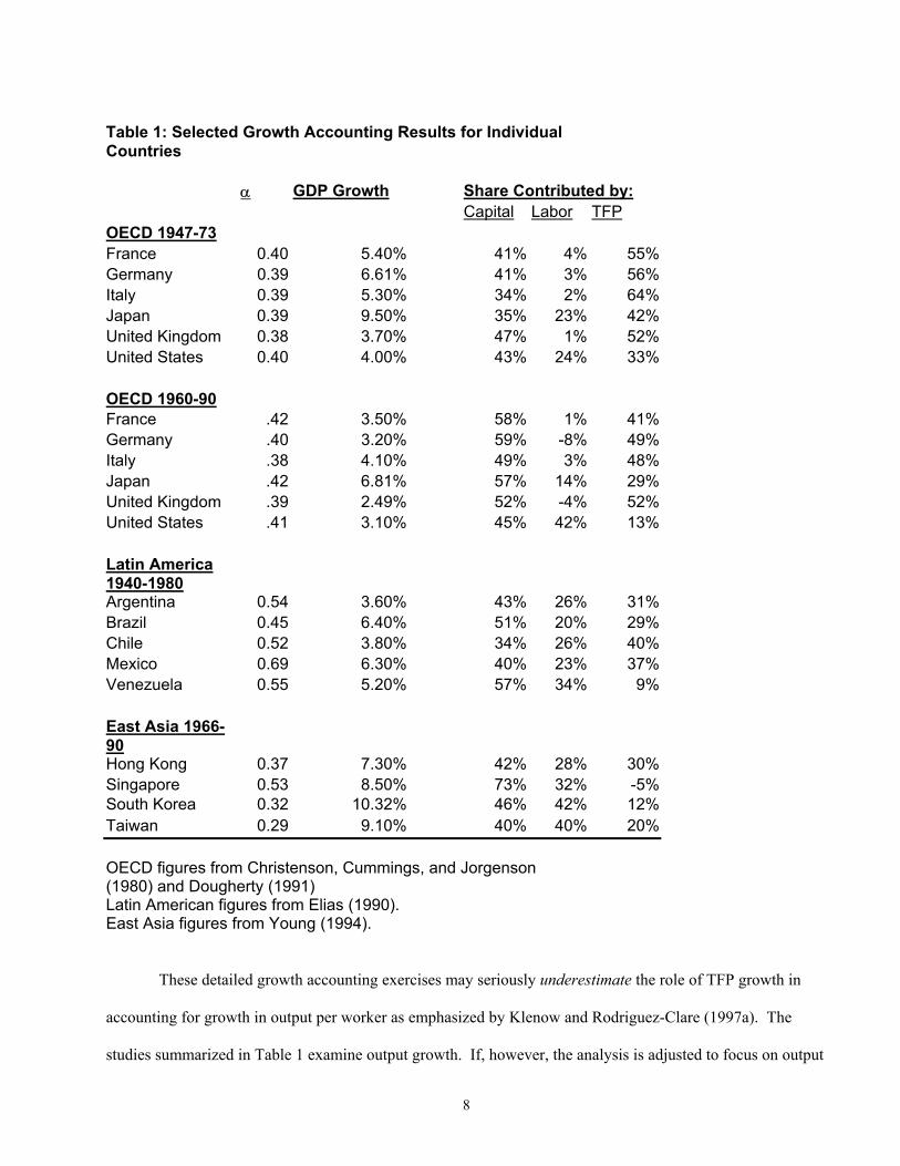
East Asian Countries. Table 1 summarizes some of these results.3 Although there are large cross-country

variations in the fraction of growth accounted for by TFP-growth, some general patterns emerge. The fraction

of output growth accounted for TFP growth hovers around 50% for OECD countries. There is greater

variation among Latin American countries, with the average accounted for by TFP growth around 30%.

Young (1994) argues that factor accumulation was a key component of the growth miracle in some East Asian

economies.

8

Table 1: Selected Growth Accounting Results for Individual Countries

α GDP Growth Share Contributed by: Capital Labor TFP

OECD 1947-73 France 0.40 5.40% 41% 4% 55% Germany 0.39 6.61% 41% 3% 56% Italy 0.39 5.30% 34% 2% 64% Japan 0.39 9.50% 35% 23% 42% United Kingdom 0.38 3.70% 47% 1% 52% United States 0.40 4.00% 43% 24% 33%

OECD 1960-90 France .42 3.50% 58% 1% 41% Germany .40 3.20% 59% -8% 49% Italy .38 4.10% 49% 3% 48% Japan .42 6.81% 57% 14% 29% United Kingdom .39 2.49% 52% -4% 52% United States .41 3.10% 45% 42% 13%

Latin America 1940-1980

Argentina 0.54 3.60% 43% 26% 31% Brazil 0.45 6.40% 51% 20% 29% Chile 0.52 3.80% 34% 26% 40% Mexico 0.69 6.30% 40% 23% 37% Venezuela 0.55 5.20% 57% 34% 9%

East Asia 1966-90

Hong Kong 0.37 7.30% 42% 28% 30% Singapore 0.53 8.50% 73% 32% -5% South Korea 0.32 10.32% 46% 42% 12% Taiwan 0.29 9.10% 40% 40% 20%

OECD figures from Christenson, Cummings, and Jorgenson (1980) and Dougherty (1991)

Latin American figures from Elias (1990). East Asia figures from Young (1994).

These detailed growth accounting exercises may seriously underestimate the role of TFP growth in

accounting for growth in output per worker as emphasized by Klenow and Rodriguez-Clare (1997a). The

studies summarized in Table 1 examine output growth. If, however, the analysis is adjusted to focus on output

9

per worker, then TFP growth accounts for a much larger share of output per worker growth than the figures

presented in Table 1. In particular, Klenow and Rodriguez-Clare (1997a) show, in an extension of Young

(1994), that factor accumulation plays the crucial role only in Singapore (a small city-state) and that none of

the other East Asian miracles suggest that factor accumulation played a dominant role in accounting for

economic growth. In addition, the share attributed to capital accumulation may be exaggerated, because it does

not take into account how much TFP growth induces capital accumulation.4 In sum, while there are cases in

which factor accumulation is very closely tied to economic success, detailed growth accounting examinations

suggest that TFP growth frequently accounts for the bulk of output per worker growth.

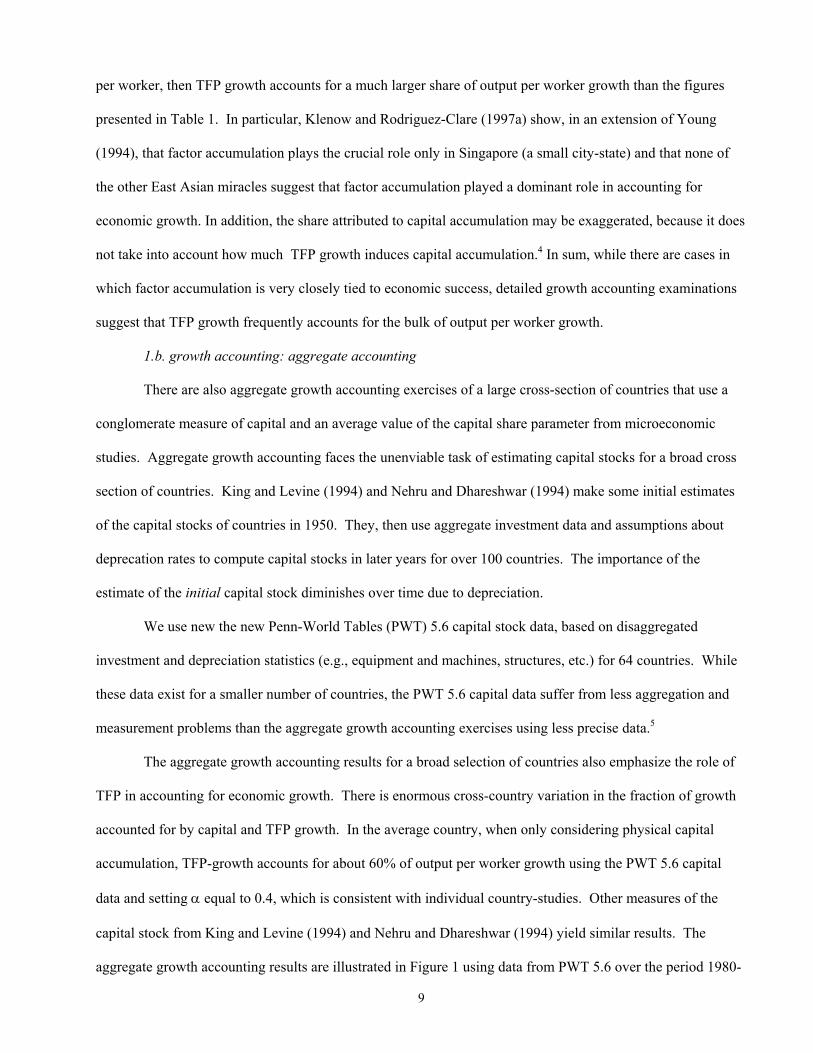
1.b. growth accounting: aggregate accounting

There are also aggregate growth accounting exercises of a large cross-section of countries that use a

conglomerate measure of capital and an average value of the capital share parameter from microeconomic

studies. Aggregate growth accounting faces the unenviable task of estimating capital stocks for a broad cross

section of countries. King and Levine (1994) and Nehru and Dhareshwar (1994) make some initial estimates

of the capital stocks of countries in 1950. They, then use aggregate investment data and assumptions about

deprecation rates to compute capital stocks in later years for over 100 countries. The importance of the

estimate of the initial capital stock diminishes over time due to depreciation.

We use new the new Penn-World Tables (PWT) 5.6 capital stock data, based on disaggregated

investment and depreciation statistics (e.g., equipment and machines, structures, etc.) for 64 countries. While

these data exist for a smaller number of countries, the PWT 5.6 capital data suffer from less aggregation and

measurement problems than the aggregate growth accounting exercises using less precise data.5

The aggregate growth accounting results for a broad selection of countries also emphasize the role of

TFP in accounting for economic growth. There is enormous cross-country variation in the fraction of growth

accounted for by capital and TFP growth. In the average country, when only considering physical capital

accumulation, TFP-growth accounts for about 60% of output per worker growth using the PWT 5.6 capital

data and setting α equal to 0.4, which is consistent with individual country-studies. Other measures of the

capital stock from King and Levine (1994) and Nehru and Dhareshwar (1994) yield similar results. The

aggregate growth accounting results are illustrated in Figure 1 using data from PWT 5.6 over the period 1980-

10

1992. We group countries into ten groups, where the countries are grouped based on output per capita growth.

The first decile represents the slowest growing group of countries. Figure 1 depicts output growth and the

dark portion indicates that part attributable to per capita capital stock growth. Figure 1 indicates that capital

growth generally accounts for less than half of output growth. Furthermore, the share of growth accounted for

by TFP growth is frequently larger in the faster growing countries. Finally, it is worth noting that there are

large differences across countries in the relationship between capital accumulation and growth. For example,

there are groups of countries for which output growth over the period 1980-1990 is negative while the capital

stock per person ratio rose through the decade. For example, Ecuador, Costa Rica, Peru, and Syria all saw real

per capita GDP fall during the 1980-1992 period at more than one percent per year, while at the same time

their real per capita capital stocks were growing at over one percent per year and educational attainment was

also increasing. Clearly, these factor injections were not being used productivity. Albeit unrepresentative,

these cases illustrate the shortcoming of focusing too heavily on factor accumulation.6

Incorporating estimates of human capital accumulation into these aggregate growth accounting

exercises does not materially alter the findings. TFP growth still, in the average country, accounts for more

than half of output per worker growth. Moreover, the data suggest a weak – and sometimes inverse –

relationship between improvements in educational attainment of the labor force and output per worker growth.

Benhabib and Spiegel (1994) and Pritchett (1996) shows that cross-country data on economic growth rates

show that increases in human capital resulting from improvements in the educational attainment of the work

force have not positively affected the growth rate of output per worker. It may be that, on average, education

does not effectively provide useful skills to workers engaged in activities that generate social returns. There is

disagreement, however. Krueger and Lindahl (1999) argue that measurement error accounts for the lack of a

relationship between growth per capita and human capital accumulation. Hanushek and Kimko (2000) find

that the quality of education is very strongly linked with economic growth. However, Klenow (1998)

demonstrates that models that highlight the role of ideas and productivity growth do a much better job of

matching the data than models that focus on the accumulation of human capital. More work is clearly needed

on the relationship between education and economic development.

11

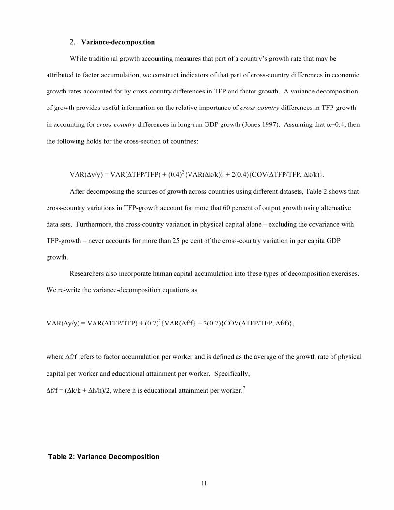
2. Variance-decomposition

While traditional growth accounting measures that part of a country’s growth rate that may be

attributed to factor accumulation, we construct indicators of that part of cross-country differences in economic

growth rates accounted for by cross-country differences in TFP and factor growth. A variance decomposition

of growth provides useful information on the relative importance of cross-country differences in TFP-growth

in accounting for cross-country differences in long-run GDP growth (Jones 1997). Assuming that α=0.4, then

the following holds for the cross-section of countries:

VAR(∆y/y) = VAR(∆TFP/TFP) + (0.4)2{VAR(∆k/k)} + 2(0.4){COV(∆TFP/TFP, ∆k/k)}.

After decomposing the sources of growth across countries using different datasets, Table 2 shows that

cross-country variations in TFP-growth account for more that 60 percent of output growth using alternative

data sets. Furthermore, the cross-country variation in physical capital alone – excluding the covariance with

TFP-growth – never accounts for more than 25 percent of the cross-country variation in per capita GDP

growth.

Researchers also incorporate human capital accumulation into these types of decomposition exercises.

We re-write the variance-decomposition equations as

VAR(∆y/y) = VAR(∆TFP/TFP) + (0.7)2{VAR(∆f/f} + 2(0.7){COV(∆TFP/TFP, ∆f/f)},

where ∆f/f refers to factor accumulation per worker and is defined as the average of the growth rate of physical

capital per worker and educational attainment per worker. Specifically,

∆f/f = (∆k/k + ∆h/h)/2, where h is educational attainment per worker.7

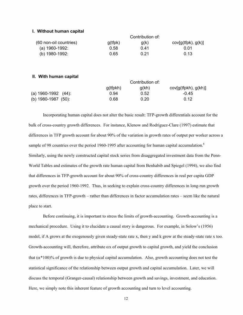
Table 2: Variance Decomposition

12

I. Without human capital

Contribution of: (60 non-oil countries) g(tfpk) g(k) cov[g(tfpk), g(k)] (a) 1960-1992: 0.58 0.41 0.01 (b) 1980-1992: 0.65 0.21 0.13

II. With human capital Contribution of: g(tfpkh) g(kh) cov[g(tfpkh), g(kh)]

(a) 1960-1992 (44): 0.94 0.52 -0.45 (b) 1980-1987 (50): 0.68 0.20 0.12

Incorporating human capital does not alter the basic result: TFP-growth differentials account for the

bulk of cross-country growth differences. For instance, Klenow and Rodriguez-Clare (1997) estimate that

differences in TFP growth account for about 90% of the variation in growth rates of output per worker across a

sample of 98 countries over the period 1960-1995 after accounting for human capital accumulation.8

Similarly, using the newly constructed capital stock series from disaggregated investment data from the Penn-

World Tables and estimates of the growth rate human capital from Benhabib and Spiegel (1994), we also find

that differences in TFP-growth account for about 90% of cross-country differences in real per capita GDP

growth over the period 1960-1992. Thus, in seeking to explain cross-country differences in long-run growth

rates, differences in TFP-growth – rather than differences in factor accumulation rates – seem like the natural

place to start.

Before continuing, it is important to stress the limits of growth-accounting. Growth-accounting is a

mechanical procedure. Using it to elucidate a causal story is dangerous. For example, in Solow’s (1956)

model, if A grows at the exogenously given steady-state rate x, then y and k grow at the steady-state rate x too.

Growth-accounting will, therefore, attribute αx of output growth to capital growth, and yield the conclusion

that (α*100)% of growth is due to physical capital accumulation. Also, growth accounting does not test the

statistical significance of the relationship between output growth and capital accumulation. Later, we will

discuss the temporal (Granger-causal) relationship between growth and savings, investment, and education.

Here, we simply note this inherent feature of growth accounting and turn to level accounting.

13

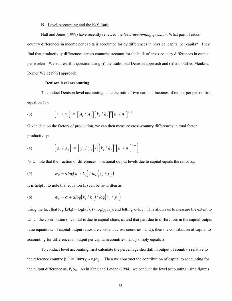
B. Level Accounting and the K/Y Ratio

Hall and Jones (1999) have recently renewed the level-accounting question: What part of cross-

country differences in income per capita is accounted for by differences in physical capital per capita? They

find that productivity differences across countries account for the bulk of cross-country differences in output

per worker. We address this question using (i) the traditional Denison approach and (ii) a modified Mankiw,

Romer Weil (1992) approach.

1. Denison level accounting

To conduct Denison level accounting, take the ratio of two national incomes of output per person from

equation (1):

(3) [ ] [ ] [ ] [ ]y y A A k k n ni i i j i j i j/ / / / = α α1−

Given data on the factors of production, we can then measure cross-country differences in total factor

productivity:

(4) [ ] [ ] [ ] [ ]{ }A A y y k k n ni j i j i j i j/ / / / / = α α1−

Now, note that the fraction of differences in national output levels due to capital equals the ratio, φki:

(5) ( ) ( )φ αki j jk y= log k log yi i/ / /

It is helpful to note that equation (5) can be re-written as

(6) ( ) ( )φ α αki j jk y= + log k log yi i/ / /

using the fact that log(ki/kj) = log(κi/κj) - log(yyi/yj), and letting κ=k/y. This allows us to measure the extent to

which the contribution of capital is due to capital share, α, and that part due to differences in the capital-output

ratio equations. If capital-output ratios are constant across countries i and j, then the contribution of capital to

accounting for differences in output per capita in countries i and j simply equals α.

To conduct level accounting, first calculate the percentage shortfall in output of country i relative to

the reference country j: Pi = 100*(yj - yi)/yj . Then we construct the contribution of capital to accounting for

the output difference as, Pi φki. As in King and Levine (1994), we conduct the level accounting using figures

14

on aggregate capital stocks, though we use the PWT 5.6 capital numbers. The world is divided into five

groups of countries ranging from the poorest to the richest. The richest group is the reference group of

countries.

Figure 2 summarizes the level accounting results: TFP-accounts for the bulk of cross-country

differences in levels of income per capita. Group 1 is the poorest group; it has more than a 90 percent shortfall

in GDP per capita from that in the reference group. The very dark area shows that part of the shortfall in

income per capita from the reference group to due to capital share of output (α) assuming that capital-output

ratios are constant. The other marked areas indicate the additional amount due to the fact that capital-output

ratios tend to rise with income per capita. TFP differences are indicated by the clear part of the bar. As

shown, TFP accounts for a large fraction of the huge differences in income per capita. Even accounting for

systematic cross-country differences in capital-output ratios, the data indicate that capital differences accounts

for less than 40% of the cross-group differences in income per capita.9

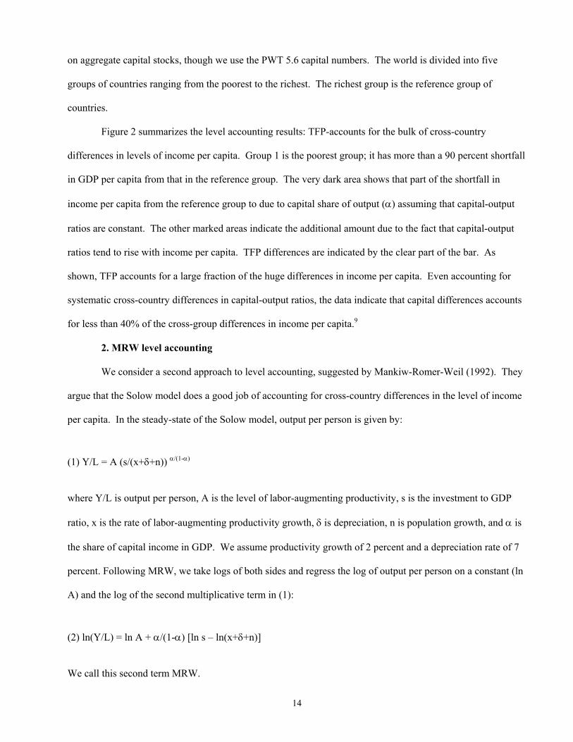
2. MRW level accounting

We consider a second approach to level accounting, suggested by Mankiw-Romer-Weil (1992). They

argue that the Solow model does a good job of accounting for cross-country differences in the level of income

per capita. In the steady-state of the Solow model, output per person is given by:

(1) Y/L = A (s/(x+δ+n)) α/(1-α)

where Y/L is output per person, A is the level of labor-augmenting productivity, s is the investment to GDP

ratio, x is the rate of labor-augmenting productivity growth, δ is depreciation, n is population growth, and α is

the share of capital income in GDP. We assume productivity growth of 2 percent and a depreciation rate of 7

percent. Following MRW, we take logs of both sides and regress the log of output per person on a constant (ln

A) and the log of the second multiplicative term in (1):

(2) ln(Y/L) = ln A + α/(1-α) [ln s – ln(x+δ+n)]

We call this second term MRW.

15

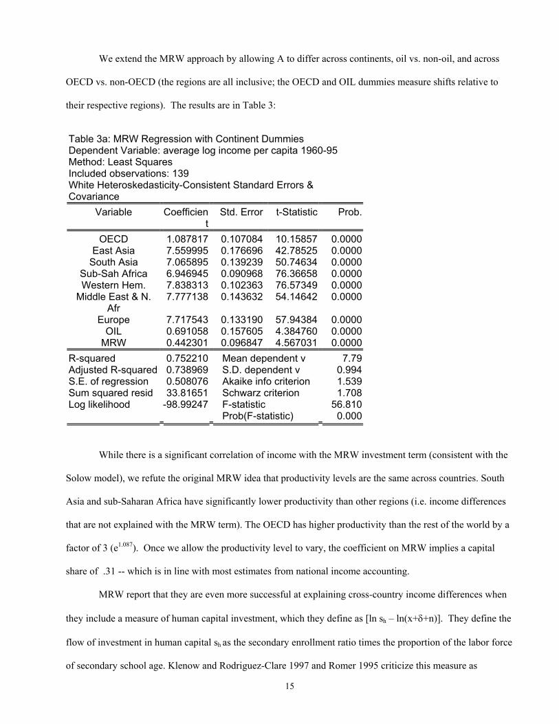
We extend the MRW approach by allowing A to differ across continents, oil vs. non-oil, and across

OECD vs. non-OECD (the regions are all inclusive; the OECD and OIL dummies measure shifts relative to

their respective regions). The results are in Table 3:

Table 3a: MRW Regression with Continent Dummies Dependent Variable: average log income per capita 1960-95 Method: Least Squares Included observations: 139 White Heteroskedasticity-Consistent Standard Errors & Covariance

Variable Coefficient

Std. Error t-Statistic Prob.

OECD 1.087817 0.107084 10.15857 0.0000 East Asia 7.559995 0.176696 42.78525 0.0000

South Asia 7.065895 0.139239 50.74634 0.0000 Sub-Sah Africa 6.946945 0.090968 76.36658 0.0000 Western Hem. 7.838313 0.102363 76.57349 0.0000

Middle East & N. Afr

7.777138 0.143632 54.14642 0.0000

Europe 7.717543 0.133190 57.94384 0.0000 OIL 0.691058 0.157605 4.384760 0.0000

MRW 0.442301 0.096847 4.567031 0.0000 R-squared 0.752210 Mean dependent v 7.79 Adjusted R-squared 0.738969 S.D. dependent v 0.994 S.E. of regression 0.508076 Akaike info criterion 1.539 Sum squared resid 33.81651 Schwarz criterion 1.708 Log likelihood -98.99247 F-statistic 56.810 Prob(F-statistic) 0.000

While there is a significant correlation of income with the MRW investment term (consistent with the

Solow model), we refute the original MRW idea that productivity levels are the same across countries. South

Asia and sub-Saharan Africa have significantly lower productivity than other regions (i.e. income differences

that are not explained with the MRW term). The OECD has higher productivity than the rest of the world by a

factor of 3 (e1.087). Once we allow the productivity level to vary, the coefficient on MRW implies a capital

share of .31 -- which is in line with most estimates from national income accounting.

MRW report that they are even more successful at explaining cross-country income differences when

they include a measure of human capital investment, which they define as [ln sh – ln(x+δ+n)]. They define the

flow of investment in human capital sh as the secondary enrollment ratio times the proportion of the labor force

of secondary school age. Klenow and Rodriguez-Clare 1997 and Romer 1995 criticize this measure as

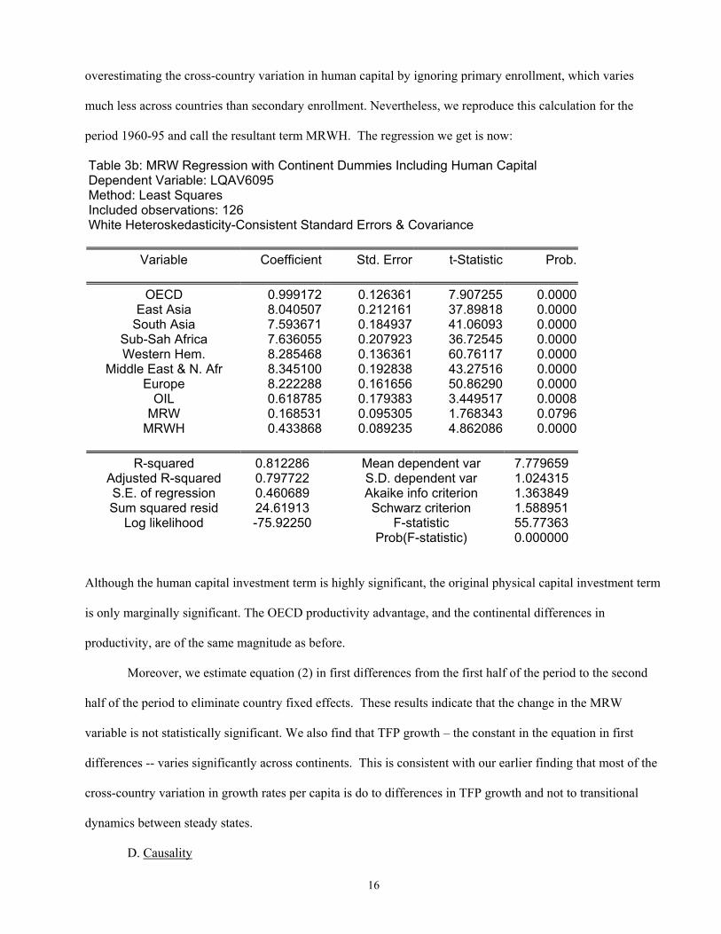
16

overestimating the cross-country variation in human capital by ignoring primary enrollment, which varies

much less across countries than secondary enrollment. Nevertheless, we reproduce this calculation for the

period 1960-95 and call the resultant term MRWH. The regression we get is now:

Table 3b: MRW Regression with Continent Dummies Including Human Capital Dependent Variable: LQAV6095 Method: Least Squares Included observations: 126 White Heteroskedasticity-Consistent Standard Errors & Covariance

Variable Coefficient Std. Error t-Statistic Prob.

OECD 0.999172 0.126361 7.907255 0.0000

East Asia 8.040507 0.212161 37.89818 0.0000 South Asia 7.593671 0.184937 41.06093 0.0000

Sub-Sah Africa 7.636055 0.207923 36.72545 0.0000 Western Hem. 8.285468 0.136361 60.76117 0.0000

Middle East & N. Afr 8.345100 0.192838 43.27516 0.0000 Europe 8.222288 0.161656 50.86290 0.0000

OIL 0.618785 0.179383 3.449517 0.0008 MRW 0.168531 0.095305 1.768343 0.0796

MRWH 0.433868 0.089235 4.862086 0.0000

R-squared 0.812286 Mean dependent var 7.779659 Adjusted R-squared 0.797722 S.D. dependent var 1.024315 S.E. of regression 0.460689 Akaike info criterion 1.363849 Sum squared resid 24.61913 Schwarz criterion 1.588951

Log likelihood -75.92250 F-statistic 55.77363 Prob(F-statistic) 0.000000

Although the human capital investment term is highly significant, the original physical capital investment term

is only marginally significant. The OECD productivity advantage, and the continental differences in

productivity, are of the same magnitude as before.

Moreover, we estimate equation (2) in first differences from the first half of the period to the second

half of the period to eliminate country fixed effects. These results indicate that the change in the MRW

variable is not statistically significant. We also find that TFP growth – the constant in the equation in first

differences -- varies significantly across continents. This is consistent with our earlier finding that most of the

cross-country variation in growth rates per capita is do to differences in TFP growth and not to transitional

dynamics between steady states.

D. Causality

17

Growth-accounting is different from causality. Factor accumulation could ignite productivity growth

and overall economic growth. Thus, factor accumulation could cause growth even though it does not account

for much the cross-country differences in growth rates or cross-country differences in the level of GDP per

capita. If this were the case, then it would be both analytically appropriate and policy-wise to focus on factor

accumulation. There is also the well-known cross-section correlation between the investment share and

growth (e.g. Levine and Renelt 1992).

Available evidence, however, suggests that physical and human capital accumulation do not cause

faster growth. For instance, Blomstrom, Lipsey, and Zejan (1996) show that output growth Granger-causes

investment. Injections of capital do not seem to be the driving force of future growth. Similarly, Carroll and

Weil (1994) show that causality tends to run from output growth to savings, not the other way around.

Evidence on human capital tells a similar story. Bils and Klenow (2000) argue that the direction of causality

runs from growth to human capital, not from human capital to growth. Thus, in terms of both physical and

human capital, the data do not provide strong support for the contention that factor accumulation ignites faster

growth in output per worker.

E. Remarks

Although there are important exceptions, as Young (1995) makes clear, “something else” besides

factor inputs accounts for the bulk cross-country differences in both income per capita and growth rates.

Furthermore, while growth-accounting does not equal causality, research also suggests that increases in factor

accumulation do not ignite faster output growth in the future. While more work is needed, available evidence

does not suggest that the direction of causality runs from physical or human capital accumulation to economic

growth in the broad cross-section of countries. Finally, measurement error may reduce the confidence that we

have in growth and level accounting. However, the residual is large in both level and growth accounting.

Also, growth and level accounting in the 1950s and 1960s produce similar estimates as those conducted in the

1990s. This implies that measurement error would have to have two systematic components: one the growth

rate of measurement error would have to be positive and large in fast growing countries and two the level

18

component of measurement error would also have to be positive and large in rich countries. While

measurement problems may play a role, a considerable body of evidence suggests that “something else”

besides factor accumulation is critical for understanding cross-country differences in the level and growth rate

of GDP per capita.

The profession gives the rather vague term “TFP” to refer to the “something else” that accounts for

growth and level differences across countries. In giving theoretical content to this residual, Grossman and

Helpman (1990), Romer (1990), Howitt 1998, and Aghion and Howitt (1992, 1998) focus on technology; that

is, better instructions for combining raw materials into useful products and services. Others take a different

approach for providing economic meaning to the “residual.” Romer (1986), Lucas (1988), and others focus on

externalities, including spillovers, economies of scale, and various complementarities in explaining the large

role played by the TFP in accounting for differences in the level and growth rates of GDP per worker.10

Alternatively, Harberger (1998) views the “residual” in terms of real cost reductions. He argues that “... there

are at least 1001 ways to reduce costs and that most of them are actually followed in one part or other of any

modern complex economy...“(p.3). He urges economists not to focus on one underlying cause of the residual

since several factors may produce real costs reductions in different sectors of the economy at different times.11

This is consistent with industry studies that reveal considerable cross-sector variation in TFP growth [Kendrick

and Grossman 1980]. Prescott (1998) also focuses on technology. He suggests that cross-country differences

in resistance to the adoption of better technologies -- arising from politics and policies -- help explain cross-

country differences in TFP.12 It would be very useful in designing models and policies to determine

empirically the relative importance of each of these conceptions of TFP.

II. Stylized Fact 2: Divergence, not Convergence, is the Big Story

Over the very long run, there has been “divergence, big time”, in the words of Pritchett (1997). Figure 3

shows that the richest nations in 1820 subsequently grew faster than the poorest countries in 1820. The ratio

of richest to poorest grew from 6 to 1 in 1820 to 70 to 1 in 1992. If we look back even further in time, the

difference between the richest and poorest countries prior to the Industrial Revolution (1700-1750) was

probably only about 2 to 1 (Bairoch 1993, p.102-6). Thus, the big story over the last 200-300 years is one of

19

massive divergence in the levels of income per capita between the rich and the poor.13 While the poor are not

getting poorer, the rich are getting richer a lot faster than the poor.

The rich continue to grow faster than the poor. Absolute divergence has continued over the last 30 years,

though not as dramatically as in earlier periods (see table 4). Also, China and India – two countries with very

large populations – have performed well recently. Nevertheless, growth differences have diverged

significantly even using recent data.14

Table 4: The rich grew most rapidly, the poor grew most slowly in 1960-92 Countries classified by income per person in 1960

Average Growth of Income per person, 1960-92

Poorest fifth of countries 1.4% Second poorest fifth of countries 1.2% Middle fifth of countries 1.8% Second richest fifth of countries 2.6% Richest fifth of countries 2.2%

Moreover, divergence understates the degree of absolute divergence over 1960-92. This is because many

countries the World Bank classified as low or middle income in the 1990s do not have complete data, while all

industrial countries have complete data. This imparts a bias towards convergence in the data like that pointed

out by DeLong 1988 regarding Baumol’s 1986 finding of convergence among industrial countries. When the

countries that are rich at the end are over-represented in the sample, this biases the sample towards

convergence. The growth rates of the lower three fifths of the sample would be even lower if we had data on

some of the disasters that were classified by the World Bank as low or middle income in the 1990s.

This tendency towards divergence if anything has become more pronounced with time. Easterly (2001)

found that the bottom half of countries ordered by per capita income in 1980 registered zero per capita growth

over 1980-98, while the top half continued to register positive growth. This was not because of divergence in

policies; this study showed that policies in poor countries converged towards those of rich countries over

1980-98.

While conditional convergence (Barro and Sala-I-Martin 1992) is certainly a feature of many cross-

economy data sets, it is difficult to look at the growing differences between the rich and poor and not focus on

20

divergence. The conditional convergence findings hold only after conditioning on an important mechanism for

divergence – spillovers from the initial level of knowledge (for which conditional convergence regressions

may be controlling with initial level of schooling). Conditional convergence also could follow mechanically

from mean reversion (Quah 1993). Since most growth models are closed economy models, it is worth looking

at what happens to convergence in closed economies. Kremer (1993) and Ades and Glaeser (1999) have found

absolute divergence in the majority of developing economies that are closed economies, suggesting an “extent

of the market” effect on growth in closed economies.

These “divergence” findings should be seen within the context of other stylized facts. Romer (1986)

shows that the growth rates of the riches countries have not been slowing over the last century. King and

Rebelo (1993) show that return to capital in the United States have not been falling over the last century.

Taken together, these observations do not naturally focus one’s attention on a model that emphasizes capital

accumulation and that has diminishing returns to factors, some fixed factor of production, and constant returns

to scale. At the same time, these observations do not provide unequivocal support for any particular

conception of what best explains the “something else” producing these stylized facts.

III. Stylized Fact 3: Growth is not persistent, growth paths are remarkably different across countries, while factor accumulation is persistent and less erratic

Growth is remarkably unstable over time. The correlation of per capita growth in 1977-92 with per capita

growth in 1960-76 across 135 countries is only .08.15 This low persistence of growth is not just a

characteristic of the postwar era. For the 25 countries that have the data, there is a correlation of only .097

across 1820-1870 and 1870-1929.16

In contrast, the cross period correlation of capital per capita growth is 0.41 For models that postulate a

linear relationship between growth and investment to GDP (thus using investment to GDP as an alternative

measure of capital accumulation), the mismatch in persistence is even worse.17 The correlation of

investment/GDP in 1977-92 with investment/GDP in 1960-76 is .85. Nor do models that postulate growth per

capita as a function of human capital accumulation do better. The correlation across 1960-76 and 1977-92 for

primary enrollment is .82, while the cross-period correlation for secondary enrollment is .91. This suggests

21

that much of the large variation of growth over time is not explained by the much smaller variation in physical

and human capital accumulation.

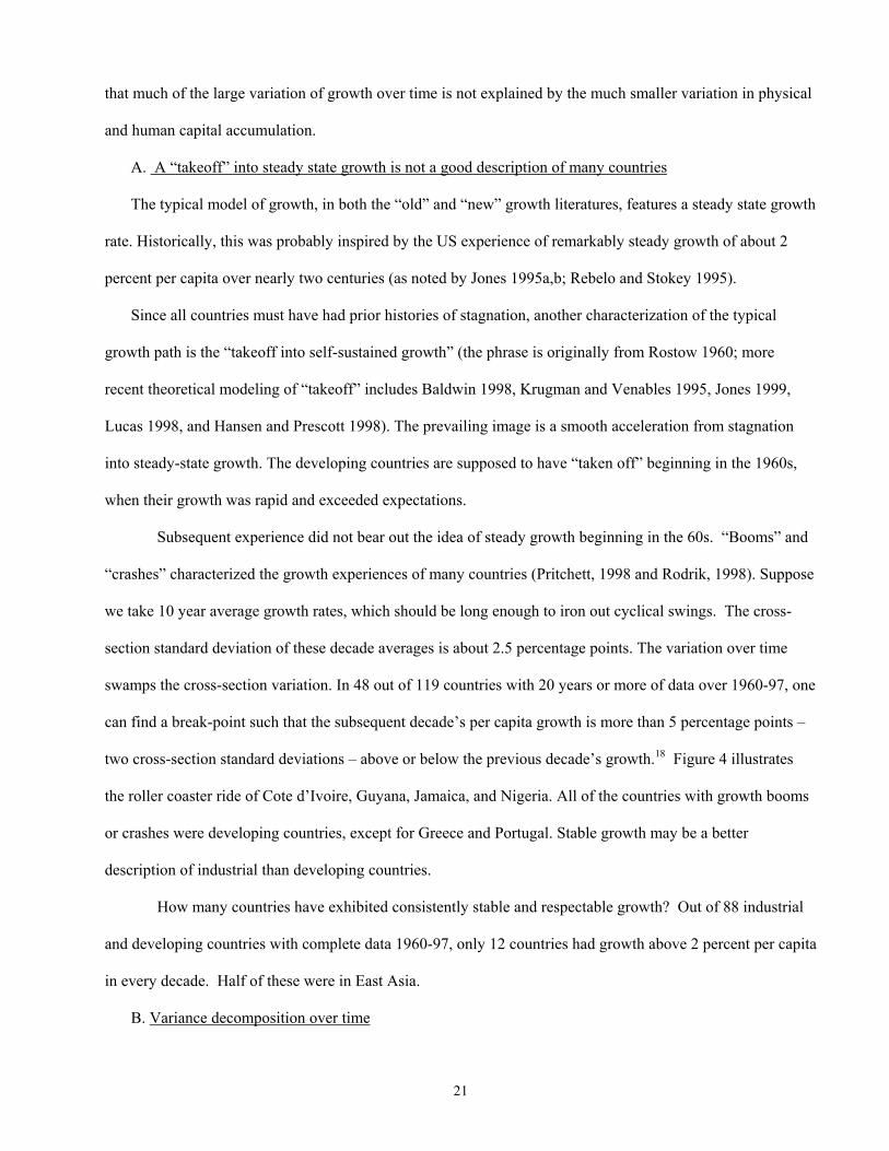
A. A “takeoff” into steady state growth is not a good description of many countries

The typical model of growth, in both the “old” and “new” growth literatures, features a steady state growth

rate. Historically, this was probably inspired by the US experience of remarkably steady growth of about 2

percent per capita over nearly two centuries (as noted by Jones 1995a,b; Rebelo and Stokey 1995).

Since all countries must have had prior histories of stagnation, another characterization of the typical

growth path is the “takeoff into self-sustained growth” (the phrase is originally from Rostow 1960; more

recent theoretical modeling of “takeoff” includes Baldwin 1998, Krugman and Venables 1995, Jones 1999,

Lucas 1998, and Hansen and Prescott 1998). The prevailing image is a smooth acceleration from stagnation

into steady-state growth. The developing countries are supposed to have “taken off” beginning in the 1960s,

when their growth was rapid and exceeded expectations.

Subsequent experience did not bear out the idea of steady growth beginning in the 60s. “Booms” and

“crashes” characterized the growth experiences of many countries (Pritchett, 1998 and Rodrik, 1998). Suppose

we take 10 year average growth rates, which should be long enough to iron out cyclical swings. The cross-

section standard deviation of these decade averages is about 2.5 percentage points. The variation over time

swamps the cross-section variation. In 48 out of 119 countries with 20 years or more of data over 1960-97, one

can find a break-point such that the subsequent decade’s per capita growth is more than 5 percentage points –

two cross-section standard deviations – above or below the previous decade’s growth.18 Figure 4 illustrates

the roller coaster ride of Cote d’Ivoire, Guyana, Jamaica, and Nigeria. All of the countries with growth booms

or crashes were developing countries, except for Greece and Portugal. Stable growth may be a better

description of industrial than developing countries.

How many countries have exhibited consistently stable and respectable growth? Out of 88 industrial

and developing countries with complete data 1960-97, only 12 countries had growth above 2 percent per capita

in every decade. Half of these were in East Asia.

B. Variance decomposition over time

22

This supposition of unstable growth is further confirmed by conducting an intertemporal variance-

decomposition exercise. This time we conduct the decomposition over time rather than across countries. In

conjunction with the cross-country variance decomposition presented above, this analysis represents a full

exploration of the panel data we have constructed on growth and its factors. Specifically, we set up a panel of

seven 5-year time periods for each country for per capita growth and physical capital per capita growth. We

then subtract off the country means and then analyze the variance using the same formula as before:

VAR(∆y/y) = VAR(∆TFP/TFP) + (0.4)2{VAR(∆k/k)} + 2(0.4){COV(∆TFP/TFP), ∆k/k)}

We find that TFP accounts for 86 percent of the intertemporal variation in overall growth. Using the

same sample of countries, we found that TFP growth accounts for 61 percent of the cross-sectional variation.

Thus, growth is much more unstable over time than physical capital growth.

Besides emphasizing the importance of TFP in explaining long-run development patterns, the findings

that growth is not persistent and that growth patterns are very different across countries complicate the

challenge for economic theorists. Existing models miss important development experiences. Some countries

grow steadily (the U.S.). Some grow steadily and then stop for long periods (Argentina). Some do not grow

for long periods and then suddenly “take off” (Korea, Thailand). Others have basically never grown

(Somalia). Sole reliance on either steady-state models or standard multiple equilibria models will have a

difficult time accounting for these very different growth experiences. Different models may be needed for

different patterns of growth across countries. Steady-state models fit the U.S. type experience. The unstable

growth cases fit more naturally multiple equilibria models, since the long-run fundamentals of countries are

stable.19

IV: Stylized Fact 4: When It Rains, It Pours

This section presents a large array of new information on the degree to which economic activity is

highly concentrated. We use cross-country data, data from counties within the United States, information from

individual developing countries, and data on international flows of capital, labor, and human capital to

examine economic concentration. This concentration has a fractal-like quality: it recurs at all levels of

23

analysis, from the global level down to the city level. This concentration suggests that some regions have

“something” that attracts all factors of production, while other regions do not.

One can speculate on the “something else” driving factor flows. Better policies in area Z than in area

Y could explain factor flows. These policies could include legal systems, property rights, political stability,

public education, infrastructure, taxes, regulations, macroeconomic stability, etc. However, these policies are

national in nature. Yet, below we document within country concentration. Externalities may play an

important role, so that factors congregate. Critically, policies differences, or externalities, or differences in

“something else” do not have to be large. Small “TFP” differences can have dramatic long-run implications.

Thus, while we do not offer a specific explanation, our results further motivate work on economic geography

as a vehicle for better understanding economic growth.

A. Concentration

At the global level, most obviously, high income status is concentrated among a small number of

nations. The top 20 nations of the world have only 15% of the world’s population but produce 50% of world

GDP. On the poverty side, the poorest half of the world’s population account for only 14% of its GDP.20

Map 1 shows the richest nations in black and the poorest in gray. These concentrations of wealth and

poverty have an ethnic and geographic dimension: 18 of the top 20 nations are in Western Europe or settled

primarily by Western Europeans. 17 of the poorest 20 nations are in tropical Africa. The richest nation in 1985

(the US) had an income 55 times that of the poorest nation (Ethiopia). Taking into account the inequality

within countries, the international income differences are even starker. The richest quintile in the US had an

income that was 528 times the income of the poorest quintile in Guinea-Bissau.

Income at the global level is highly concentrated in space also. Sorting by GDP per square kilometer,

the densest 10% of the worlds land area accounts for 54% of its GDP; the least dense half of nations’ land area

produces only 11% of World GDP. 21

These calculations are done assuming that income is evenly spread among people and land area within

nations, and so understate the degree of concentration. When we look within nations, we find high

concentration of wealth and poverty also. We illustrate here with the nation where we found the most detailed

data: the United States.

24

We used the database of 3141 counties in the US to examine income and poverty concentration.

Sorting counties by GDP per square mile, we found a 50 and 2 rule: 50 percent of GDP is produced in counties

that account for only 2 percent of the land, while the least dense counties that account for 50 percent of the

land produce only 2 percent of GDP. Nor is this result just a consequence of the large unsettled areas of the

West and Alaska. If we do the same calculation for land east of the Mississippi, we still have extreme

concentration: 50 percent of GDP is produced on 4 percent of the land. The densest county is New York NY,

which has a GDP per square mile of $1.5 billion. This is about 55,000 times more than the least dense county

east of the Mississippi ($27 thousand per square mile in Keweenaw MI). Even this understates the degree of

concentration since even the most casual empiricism detects rich and poor areas within a given county (New

York county contains Harlem as well as Wall Street).

Map 2 shows these concentrations of counties accounting for half of US GDP. Obviously, another

name for these concentrations is “cities.” This concentration is explained by the fact that most economic

activity takes place in densely populated metropolitan areas. Metropolitan counties are $3300 richer per person

than rural counties (the difference is statistically significant, with a t-statistic of 29). More generally, there is a

strong correlation between per capita income of US counties and their population density (correlation

coefficient of .48 for the log of both concepts, with a t-statistic of 30 on the bivariate association). But even if

we restrict the sample to metropolitan counties we see concentration: 50 percent of metropolitan GDP is

produced in counties accounting for only 6 percent of metropolitan land area.22

There are also regional income differences between metropolitan areas. Metropolitan areas in the

Boston-to-Washington corridor have a per capita income that is $5874 higher on average than other

metropolitan areas. This is a huge difference: it is equal to 2.4 standard deviations in the metropolitan area

sample. Although there may be differences in the cost of living, they are unlikely to be so large as to explain

this difference. (The rent component of the cost of living may reflect either the productivity or the amenity

advantages of the area – it seems unlikely that amenities are different enough among areas to explain these

differences).

There are other possible explanations of geographic concentration, like inherent geographic

advantages of some areas. Like Mellinger, Sachs and Gallup 1999, Rappaport and Sachs 1999 argue that

25

spatial concentration of activity in the US has much to do with access to the coast. However, casual

observation suggests high concentration even within coastal areas (there are sections of the BosWash corridor

where you cannot get a radio station on the dial). It also could come about because of high transport costs and

low congestion costs (Krugman 1991, 1995, 1998, Fujita, Krugman, and Venables 1999). However, these

latter authors also point to locations of particular industries in certain locales (the Silicon Valley phenomenon)

as evidence of other types of geographic spillovers, including technology spillovers and specialized producer

services that have high fixed costs. And the high rents in downtown metropolitan areas suggest congestion

costs are very significant. As Lucas 1988 says, “what can people be paying Manhattan or downtown Chicago

rents for, if not for being near other people?”

B. Poor areas

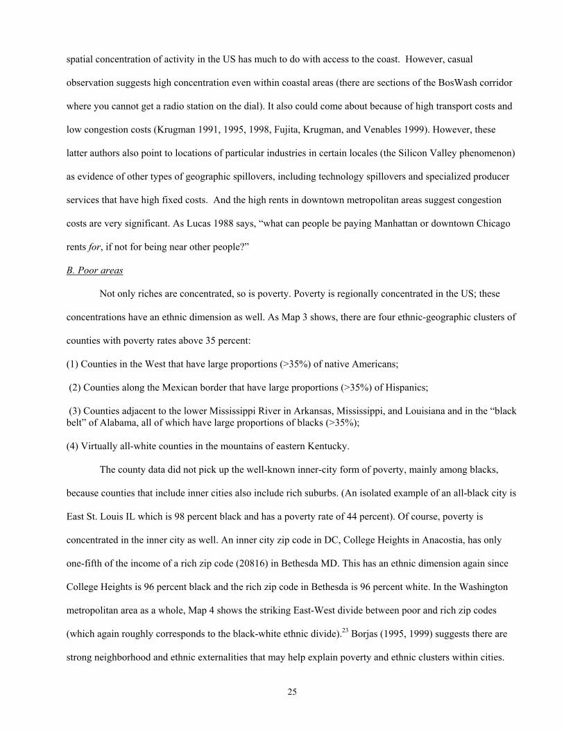
Not only riches are concentrated, so is poverty. Poverty is regionally concentrated in the US; these

concentrations have an ethnic dimension as well. As Map 3 shows, there are four ethnic-geographic clusters of

counties with poverty rates above 35 percent:

(1) Counties in the West that have large proportions (>35%) of native Americans; (2) Counties along the Mexican border that have large proportions (>35%) of Hispanics; (3) Counties adjacent to the lower Mississippi River in Arkansas, Mississippi, and Louisiana and in the “black belt” of Alabama, all of which have large proportions of blacks (>35%); (4) Virtually all-white counties in the mountains of eastern Kentucky. The county data did not pick up the well-known inner-city form of poverty, mainly among blacks,

because counties that include inner cities also include rich suburbs. (An isolated example of an all-black city is

East St. Louis IL which is 98 percent black and has a poverty rate of 44 percent). Of course, poverty is

concentrated in the inner city as well. An inner city zip code in DC, College Heights in Anacostia, has only

one-fifth of the income of a rich zip code (20816) in Bethesda MD. This has an ethnic dimension again since

College Heights is 96 percent black and the rich zip code in Bethesda is 96 percent white. In the Washington

metropolitan area as a whole, Map 4 shows the striking East-West divide between poor and rich zip codes

(which again roughly corresponds to the black-white ethnic divide).23 Borjas (1995, 1999) suggests there are

strong neighborhood and ethnic externalities that may help explain poverty and ethnic clusters within cities.

26

Sorting 1990 census tracts by percent of blacks, the census tracts with the highest shares of blacks account for

fifty percent of the black population but contain only one percent of the white population.24 While this

segregation by race and class could simply reflect the preferences of rich white people to live next to each

other, economists usually prefer to offer economic motivations rather than exogenous preferences as

explanations of economic phenomena. Benabou (1993, 1996) stresses the endogenous sorting between rich

and poor for the rich to take advantage of externalities like locally funded schools.

Poverty areas exist in many countries: northeast Brazil, southern Italy, Chiapas in Mexico, Balochistan

in Pakistan, and the Atlantic Provinces in Canada. Researchers have found externalities to be part of the

explanation of these poverty clusters. Bouillon, Legovini and Lustig 1999 find that there is a negative Chiapas

effect in Mexican household income data, and that this effect has gotten worse over time. Households in the

poor region of Tangail/Jamalpur in Bangladesh earned less than identical households in the better off region of

Dhaka (Ravallion and Wodon 1998). Ravallion and Jalan (1996) and Jalan and Ravallion (1997) likewise

found that households in poor counties in southwest China earned less than households with identical human

capital and other characteristics in rich Guangdong Province. Rauch 1993 likewise found with US data that

individuals with identical characteristics earn less in low human capital cities than in high human capital cities.

C. Ethnic differentials

Some theories stress in-group externalities (Borjas 1992, 1995, 1999, Benabou 1993, 1996). Poverty

and riches are also concentrated in certain ethnic groups; it would not be appealing to explain these differences

by exogenous savings preferences. While other stories like discrimination and intergenerational transmission

could explain ethnic differences, in terms of growth models they seem more consistent with in-group

spillovers than with individual factor accumulation.

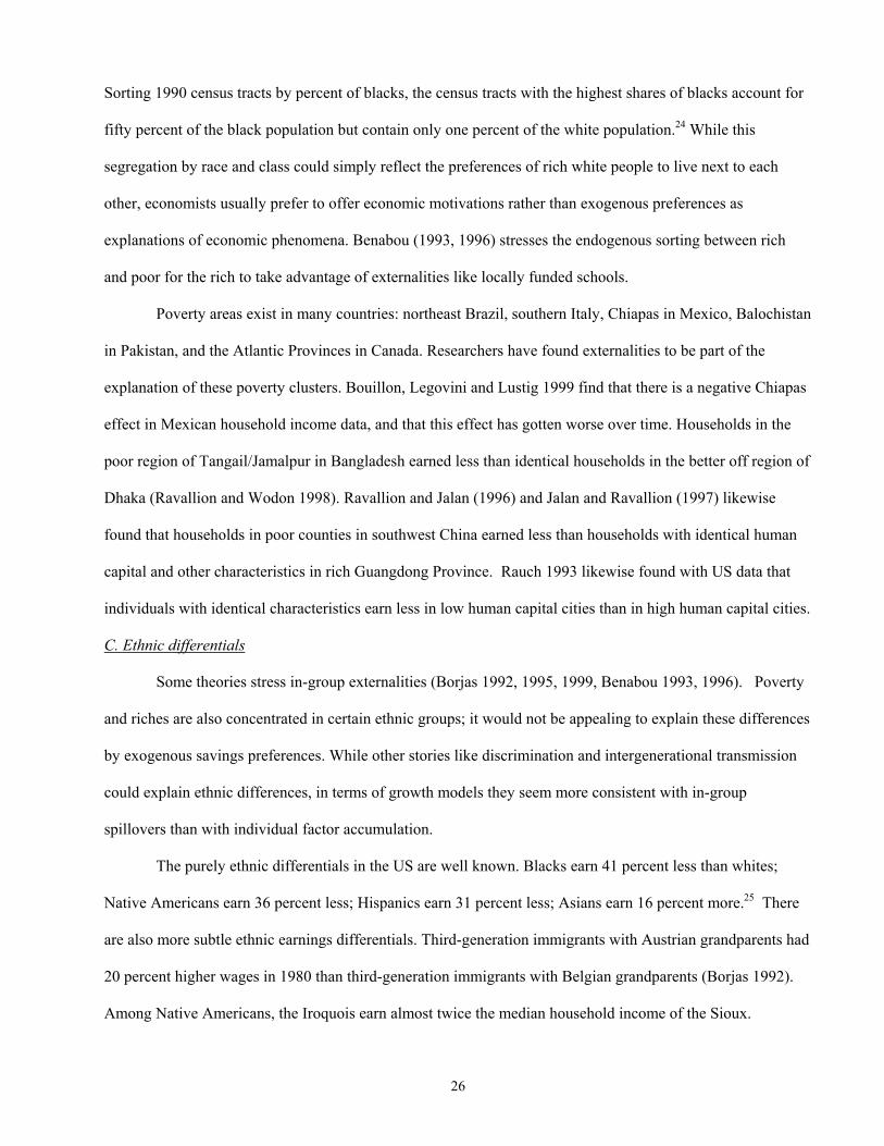
The purely ethnic differentials in the US are well known. Blacks earn 41 percent less than whites;

Native Americans earn 36 percent less; Hispanics earn 31 percent less; Asians earn 16 percent more.25 There

are also more subtle ethnic earnings differentials. Third-generation immigrants with Austrian grandparents had

20 percent higher wages in 1980 than third-generation immigrants with Belgian grandparents (Borjas 1992).

Among Native Americans, the Iroquois earn almost twice the median household income of the Sioux.

27

Other ethnic differentials appear by religion. Episcopalians earn 31% more income than Methodists

(Kosmin and Lachman, 1993, p. 260) Twenty-three percent of the Forbes 400 richest Americans are Jewish,

although only two percent of the US population is Jewish (Lipset 1997).26

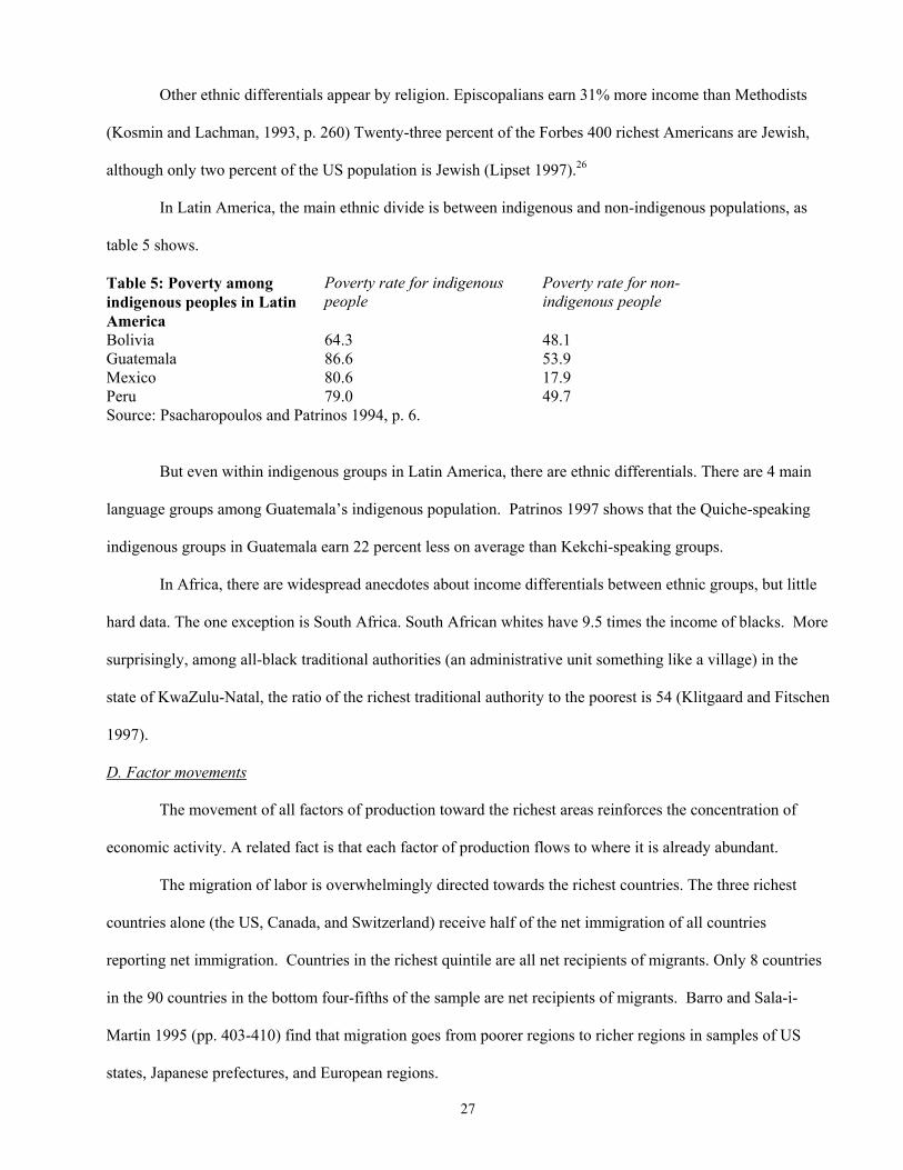
In Latin America, the main ethnic divide is between indigenous and non-indigenous populations, as

table 5 shows.

Table 5: Poverty among indigenous peoples in Latin America

Poverty rate for indigenous people

Poverty rate for non-indigenous people

Bolivia 64.3 48.1 Guatemala 86.6 53.9 Mexico 80.6 17.9 Peru 79.0 49.7 Source: Psacharopoulos and Patrinos 1994, p. 6.

But even within indigenous groups in Latin America, there are ethnic differentials. There are 4 main

language groups among Guatemala’s indigenous population. Patrinos 1997 shows that the Quiche-speaking

indigenous groups in Guatemala earn 22 percent less on average than Kekchi-speaking groups.

In Africa, there are widespread anecdotes about income differentials between ethnic groups, but little

hard data. The one exception is South Africa. South African whites have 9.5 times the income of blacks. More

surprisingly, among all-black traditional authorities (an administrative unit something like a village) in the

state of KwaZulu-Natal, the ratio of the richest traditional authority to the poorest is 54 (Klitgaard and Fitschen

1997).

D. Factor movements

The movement of all factors of production toward the richest areas reinforces the concentration of

economic activity. A related fact is that each factor of production flows to where it is already abundant.

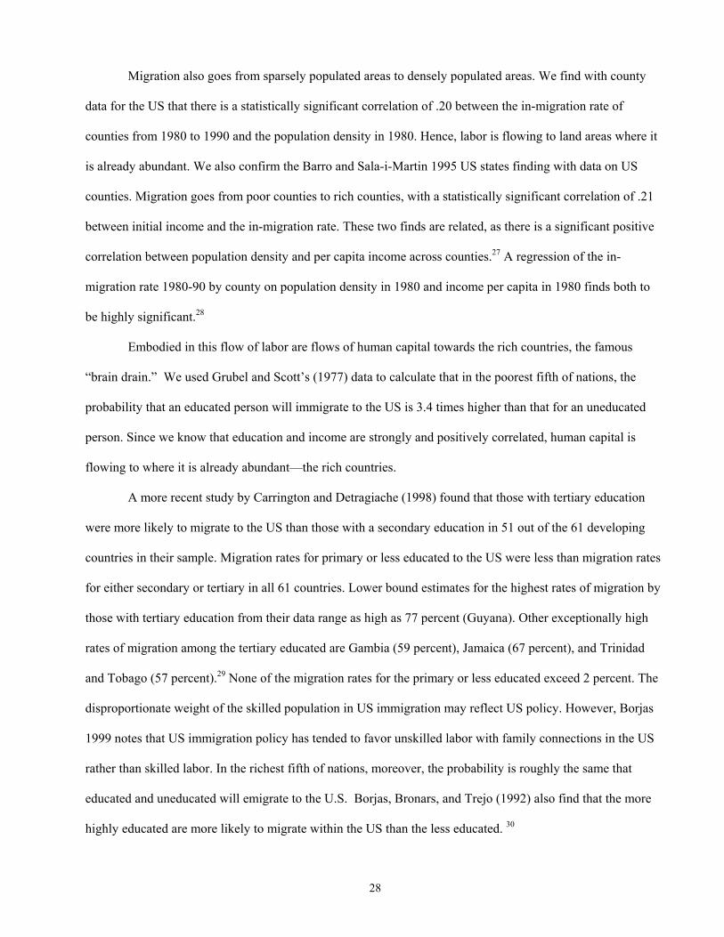
The migration of labor is overwhelmingly directed towards the richest countries. The three richest

countries alone (the US, Canada, and Switzerland) receive half of the net immigration of all countries

reporting net immigration. Countries in the richest quintile are all net recipients of migrants. Only 8 countries

in the 90 countries in the bottom four-fifths of the sample are net recipients of migrants. Barro and Sala-i-

Martin 1995 (pp. 403-410) find that migration goes from poorer regions to richer regions in samples of US

states, Japanese prefectures, and European regions.

28

Migration also goes from sparsely populated areas to densely populated areas. We find with county

data for the US that there is a statistically significant correlation of .20 between the in-migration rate of

counties from 1980 to 1990 and the population density in 1980. Hence, labor is flowing to land areas where it

is already abundant. We also confirm the Barro and Sala-i-Martin 1995 US states finding with data on US

counties. Migration goes from poor counties to rich counties, with a statistically significant correlation of .21

between initial income and the in-migration rate. These two finds are related, as there is a significant positive

correlation between population density and per capita income across counties.27 A regression of the in-

migration rate 1980-90 by county on population density in 1980 and income per capita in 1980 finds both to

be highly significant.28

Embodied in this flow of labor are flows of human capital towards the rich countries, the famous

“brain drain.” We used Grubel and Scott’s (1977) data to calculate that in the poorest fifth of nations, the

probability that an educated person will immigrate to the US is 3.4 times higher than that for an uneducated

person. Since we know that education and income are strongly and positively correlated, human capital is

flowing to where it is already abundant—the rich countries.

A more recent study by Carrington and Detragiache (1998) found that those with tertiary education

were more likely to migrate to the US than those with a secondary education in 51 out of the 61 developing

countries in their sample. Migration rates for primary or less educated to the US were less than migration rates

for either secondary or tertiary in all 61 countries. Lower bound estimates for the highest rates of migration by

those with tertiary education from their data range as high as 77 percent (Guyana). Other exceptionally high

rates of migration among the tertiary educated are Gambia (59 percent), Jamaica (67 percent), and Trinidad

and Tobago (57 percent).29 None of the migration rates for the primary or less educated exceed 2 percent. The

disproportionate weight of the skilled population in US immigration may reflect US policy. However, Borjas

1999 notes that US immigration policy has tended to favor unskilled labor with family connections in the US

rather than skilled labor. In the richest fifth of nations, moreover, the probability is roughly the same that

educated and uneducated will emigrate to the U.S. Borjas, Bronars, and Trejo (1992) also find that the more

highly educated are more likely to migrate within the US than the less educated. 30

29

Capital also flows mainly to areas that are already rich, as famously pointed out by Lucas 1990. In

1990, the richest 20 percent of world population received 92 percent of portfolio capital gross inflows; the

poorest 20 percent received 0.1 percent of portfolio capital inflows. The richest 20 percent of the world

population received 79 percent of foreign direct investment; the poorest 20 percent received 0.7 percent of

foreign direct investment. Altogether, the richest 20 percent of the world population received 88 percent of

private capital gross inflows; the poorest 20 percent received 1 percent of private capital gross inflows.

E. Evidence on skill premia and human capital

Critically, skilled workers earn less, rather than more, in poor countries. This seems inconsistent with

the open economy version of the neoclassical factor accumulation model by Barro, Mankiw, and Sala-i-Martin

(BMS) 1995. In the BMS model, capital flows equalize the rate of return to physical capital across countries,

while human capital is immobile. Immobile human capital explains the difference in per worker income

across nations in BMS. As pointed out by Romer 1995, this implies that both the skilled wage and the skill

premium should be much higher in poor countries than in rich countries. To illustrate this, we specify a

standard production function for country i as βαβα −−= 1

iiii HLAKY

Assuming technology (A) is the same across countries and that rates of return to physical capital are equated

across countries, we can solve for the ratio of the skilled wage in country i to that in country j, as a function of

their per capita incomes, as follows:

βαβ−−

−

=

∂

∂∂∂

1

//

jj

ii

j

j

i

i

LYLY

HYHY

Using the physical and human capital shares (.3 and .5 respectively) suggested by Mankiw 1995, we

calculate that skilled wages should be five times greater in India than the US (to correspond to a fourteen-fold

difference in per capita income). In general, the equation above shows that skilled wages differences across

countries should be inversely related to per capita income if human capital abundance explains income

differences across countries, a la BMS.

30

The skill premium should be seventy times higher in India than the US. If the ratio of skilled to

unskilled wage is about 2 in the US, then the skilled to unskilled wage ratio in India should be 140. This would

imply a fantastic rate of return to education in India, seventy times larger than the return to education in the

US.

The facts do not support these predictions: skilled workers earn more in rich countries. Fragmentary

data from wage surveys say that engineers earn an average of $55,000 in New York compared to $2,300 in

Bombay (Union Bank of Switzerland 1994). Instead of skilled wages being five times higher in India than in

the US, skilled wages are 24 times higher in the US than in India. The higher wages across all occupational

groups is consistent with a higher “A” in the US than in India. Figure 5 shows that the skilled wage (proxied

by salaries of engineers, adjusted for purchasing power) is positively associated with per capita income across

countries, as a productivity explanation of income differences would imply, and not negatively correlated, as a

BMS human capital explanation of income differences would imply. The correlation between skilled wages

and per capita income across 44 countries is .81.

Within India, the wage of engineers is only about 3 times the wage of building laborers. Rates of

return to education are also only about twice as high in poor countries – about eleven percent versus six

percent from low income to high income (Psacharopolous 1994, p. 1332) – not 42 times higher. Consistent

with this evidence, we have also seen that the incipient flow of human capital, despite barriers to immigration,

is toward the rich countries.

F. Evaluating Growth Models Since Riches and Poverty are Concentrated

The high concentration of income, reinforced by the flow of all factors towards the richest areas, is

inconsistent with the neoclassical growth model. The distribution of income across space and across people at

all levels is highly skewed to the right (skewness coefficient of 2.58 across countries in 1980, skewness across

US cities of 2.2, and skewness across US counties of 1.60 in 1990, where 0 is symmetry). There is no reason to

think that the determinants of income in the neoclassical model (saving, population growth) are skewed to the

right, while models of technological complementarities (e.g. Kremer 1993) can explain this skewness.

Moreover, the concentration of all factors in the rich, densely populated areas even within countries is

incompatible with a version of the neoclassical model that includes land as a factor of production. With land in

31

fixed supply, physical and human capital and labor should all want to flow to areas abundant in land (adjusting

for land quality) but scarce in other factors.

Furthermore, in the neoclassical model physical and human capital should flow from rich to poor

areas, while unskilled labor moves from poor to rich. In fact, we find physical and human capital flowing

toward already rich areas, while unskilled labor is less mobile but also tends to flow to rich countries. This is

inconsistent with the neoclassical model as presented by Mankiw, Romer, and Weil 1992.

Stylized Fact #4 concurs with Klenow and Rodriguez-Clare (1997) that the “neoclassical revival in

growth economics” has “gone too far.” The neoclassical model has no explanation for why riches and poverty

are concentrated in certain regions within countries. The neoclassical model also does not explain why there

are such pronounced income differences between ethnic groups. Stylized Fact #4 is consistent with poverty

trap models like those of Azariadis and Drazen (1991), Becker, Murphy, and Tamura (1990), Kremer (1993),

and Murphy, Shleifer, and Vishny (1989). It is also consistent with models of in-group ethnic and

neighborhood externalities (Borjas 1992, 1995, 1999, Benabou 1993, 1996) and geographic externalities

(Krugman 1991, 1995, 1998, Fujita, Krugman, and Venables 1999).

Stylized Fact #4 also seems to be more consistent with a productivity explanation of income

differences than with a factor accumulation story. If a rich area is rich because A is higher, then all factors of

production will tend to flow toward this rich area, reinforcing the concentration. Spillovers between agents

also seem more natural with technological models of growth, since technological knowledge is inherently

more non-rival and more non-excludable than factor accumulation. Technological spillovers between agents

will lead to endogenous matching of rich agents with each other, while their matches will reinforce the poverty

of the poor with other poor people (as in the O-ring story of Kremer 1993 or the inequality model of Benabou

1996). A better understanding of economic geography and externalities would help shape models of economic

growth.

V. Stylized Fact 5: Policy Matters

The empirical literature on national policies and economic growth is huge. There is considerable

disagreement about which policies are most strongly linked with economic growth. Some authors focus on

openness to international trade (Frankel and Romer, 1999), others on fiscal policy (Easterly and Rebelo, 1993),

32

others on financial development (Levine, Loayza, and Beck, 2000), and others on macroeconomic policies

(Fischer 1993. These papers have at least one common feature: they all find that some indicator of national

policy is strongly linked with economic growth, which confirms the argument made by Levine and Renelt

(1992).

The purpose of this section is to use recent econometric techniques to examine the linkages between

economic growth and a range of national policies. Specifically, most empirical assessments of the growth-

policy relationship are plagued by three shortcomings. First, existing work does not generally confront the

issue of endogeneity. Moreover, even when authors use instrumental variables, they frequently assume that

many of the regressors are exogenous and only focus on the potential endogeneity of one variable of interest.

By not fully confronting the issue of causality, existing work may produce biased assessments. Second,

traditional cross-country regressions may suffer from omitted variable bias. That is, cross-country growth

regressions may omit an important country-specific effect and thereby produce biased coefficient estimates.

Third, almost all cross-country regressions included lagged real per capital GDP as a regressor. Since the

dependent variable is the growth rate of real per capita GDP, this specification may produce biased coefficient

estimates. This paper uses new statistical procedures that ameliorate these potential biases so that we can draw

more accurate inferences on the impact of national policies on economic growth.

The purpose of this paper is not to identify the most important policies influencing growth. Besides

remaining disagreements among the authors of this paper regarding this question, this paper compiles key

stylized facts associated with long-run growth. By employing the latest econometric techniques, we confirm

earlier findings that national policies are strongly linked with economic growth. The regression results are

consistent with policies having significant long-run effects on national growth rates or on steady-state levels of

national output. Furthermore, the regression results show that national policies are strongly linked with TFP

growth (Beck, Levine, and Loayza, 2000)

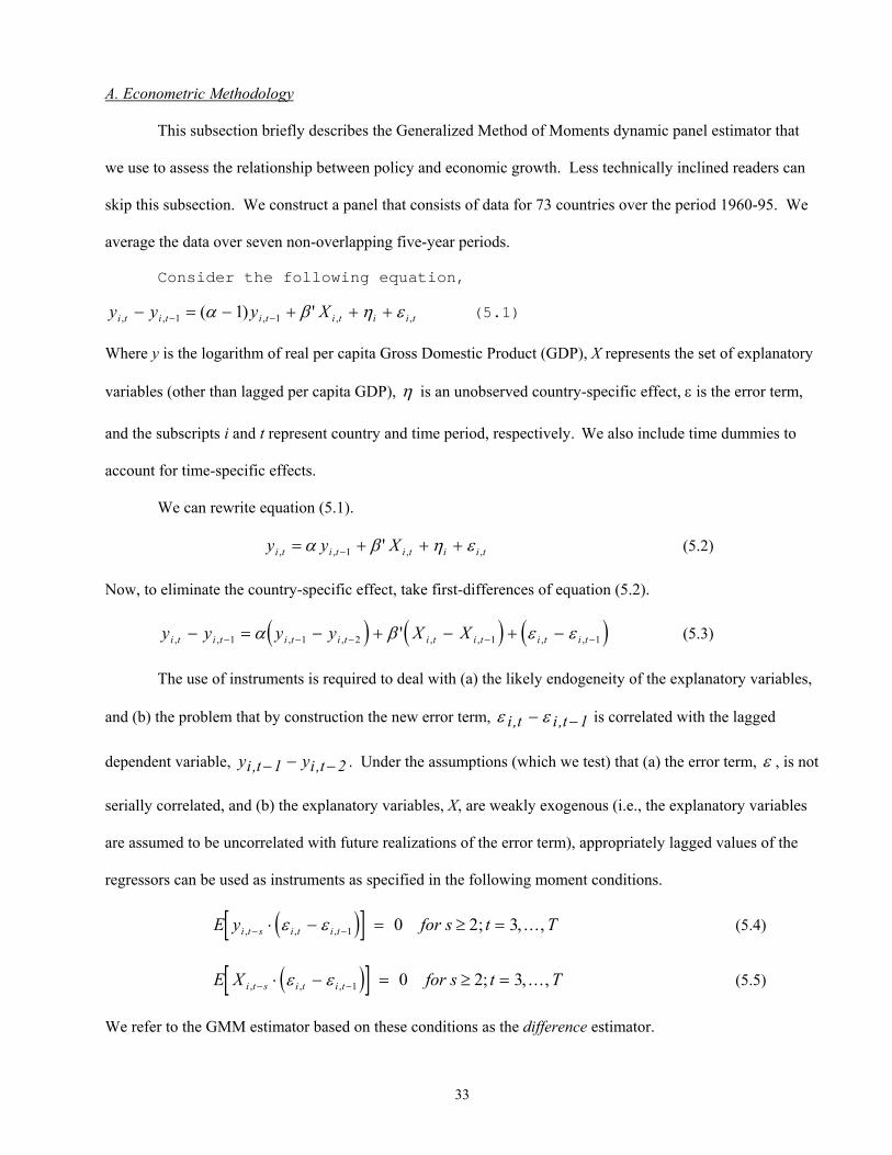
33

A. Econometric Methodology

This subsection briefly describes the Generalized Method of Moments dynamic panel estimator that

we use to assess the relationship between policy and economic growth. Less technically inclined readers can

skip this subsection. We construct a panel that consists of data for 73 countries over the period 1960-95. We

average the data over seven non-overlapping five-year periods.

Consider the following equation,

y y y Xi t i t i t i t i i t, , , , ,( ) '− = − + + +− −1 11α β η ε (5.1)

Where y is the logarithm of real per capita Gross Domestic Product (GDP), X represents the set of explanatory

variables (other than lagged per capita GDP), η is an unobserved country-specific effect, ε is the error term,

and the subscripts i and t represent country and time period, respectively. We also include time dummies to

account for time-specific effects.

We can rewrite equation (5.1).

y y Xi t i t i t i i t, , , ,'= + + +−α β η ε 1 (5.2)

Now, to eliminate the country-specific effect, take first-differences of equation (5.2).

( ) ( ) ( )y y y y X Xi t i t i t i t i t i t i t i t, , , , , , , ,'− = − + − + −− − − − −1 1 2 1 1α β ε ε (5.3)

The use of instruments is required to deal with (a) the likely endogeneity of the explanatory variables,

and (b) the problem that by construction the new error term, ε εi t i t, ,− −1 is correlated with the lagged

dependent variable, y yi t i t, ,− −−1 2 . Under the assumptions (which we test) that (a) the error term, ε , is not

serially correlated, and (b) the explanatory variables, X, are weakly exogenous (i.e., the explanatory variables

are assumed to be uncorrelated with future realizations of the error term), appropriately lagged values of the

regressors can be used as instruments as specified in the following moment conditions.

( )[ ]E y for s t Ti t s i t i t, , , ; , ...,− −⋅ − = ≥ =ε ε 1 0 2 3 (5.4)

( )[ ]E X for s t Ti t s i t i t, , , ; , ...,− −⋅ − = ≥ =ε ε 1 0 2 3 (5.5)

We refer to the GMM estimator based on these conditions as the difference estimator.

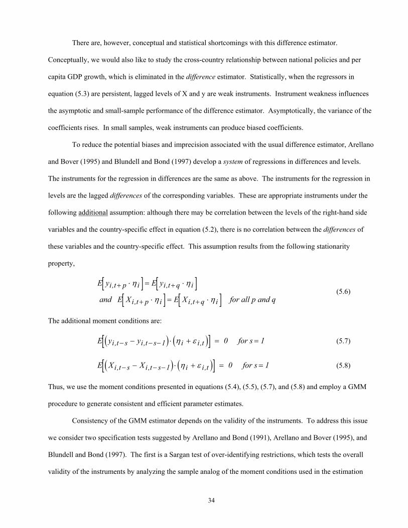
34

There are, however, conceptual and statistical shortcomings with this difference estimator.

Conceptually, we would also like to study the cross-country relationship between national policies and per

capita GDP growth, which is eliminated in the difference estimator. Statistically, when the regressors in

equation (5.3) are persistent, lagged levels of X and y are weak instruments. Instrument weakness influences

the asymptotic and small-sample performance of the difference estimator. Asymptotically, the variance of the

coefficients rises. In small samples, weak instruments can produce biased coefficients.

To reduce the potential biases and imprecision associated with the usual difference estimator, Arellano

and Bover (1995) and Blundell and Bond (1997) develop a system of regressions in differences and levels.

The instruments for the regression in differences are the same as above. The instruments for the regression in

levels are the lagged differences of the corresponding variables. These are appropriate instruments under the

following additional assumption: although there may be correlation between the levels of the right-hand side

variables and the country-specific effect in equation (5.2), there is no correlation between the differences of

these variables and the country-specific effect. This assumption results from the following stationarity

property,

[ ] [ ]

[ ] [ ]E y E y

and E X E X for all p and q

i t p i i t q i

i t p i i t q i

, ,

, ,

+ +

+ +

⋅ = ⋅

⋅ = ⋅

η η

η η (5.6)

The additional moment conditions are:

( ) ( )[ ]E y y for si t s i t s i i t, , ,− − −− ⋅ + = =1 0 1η ε (5.7)

( ) ( )[ ]E X X for si t s i t s i i t, , ,− − −− ⋅ + = =1 0 1η ε (5.8)

Thus, we use the moment conditions presented in equations (5.4), (5.5), (5.7), and (5.8) and employ a GMM

procedure to generate consistent and efficient parameter estimates.

Consistency of the GMM estimator depends on the validity of the instruments. To address this issue

we consider two specification tests suggested by Arellano and Bond (1991), Arellano and Bover (1995), and

Blundell and Bond (1997). The first is a Sargan test of over-identifying restrictions, which tests the overall

validity of the instruments by analyzing the sample analog of the moment conditions used in the estimation

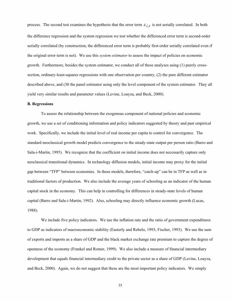
35

process. The second test examines the hypothesis that the error term ε i t, is not serially correlated. In both

the difference regression and the system regression we test whether the differenced error term is second-order

serially correlated (by construction, the differenced error term is probably first-order serially correlated even if

the original error term is not). We use this system estimator to assess the impact of policies on economic

growth. Furthermore, besides the system estimator, we conduct all of these analyses using (1) purely cross-

section, ordinary-least-squares regressions with one observation per country, (2) the pure different estimator

described above, and (30 the panel estimator using only the level component of the system estimator. They all

yield very similar results and parameter values (Levine, Loayza, and Beck, 2000).

B. Regressions

To assess the relationship between the exogenous component of national policies and economic

growth, we use a set of conditioning information and policy indicators suggested by theory and past empirical

work. Specifically, we include the initial level of real income per capita to control for convergence. The

standard neoclassical growth model predicts convergence to the steady-state output per person ratio (Barro and

Sala-i-Martin, 1995). We recognize that the coefficient on initial income does not necessarily capture only

neoclassical transitional dynamics. In technology diffusion models, initial income may proxy for the initial

gap between “TFP” between economies. In these models, therefore, “catch-up” can be in TFP as well as in

traditional factors of production. We also include the average years of schooling as an indicator of the human

capital stock in the economy. This can help in controlling for differences in steady-state levels of human

capital (Barro and Sala-i-Martin, 1992). Also, schooling may directly influence economic growth (Lucas,

1988).

We include five policy indicators. We use the inflation rate and the ratio of government expenditures

to GDP as indicators of macroeconomic stability (Easterly and Rebelo, 1993; Fischer, 1993). We use the sum

of exports and imports as a share of GDP and the black market exchange rate premium to capture the degree of

openness of the economy (Frankel and Romer, 1999). We also include a measure of financial intermediary

development that equals financial intermediary credit to the private sector as a share of GDP (Levine, Loayza,

and Beck, 2000). Again, we do not suggest that these are the most important policy indicators. We simply

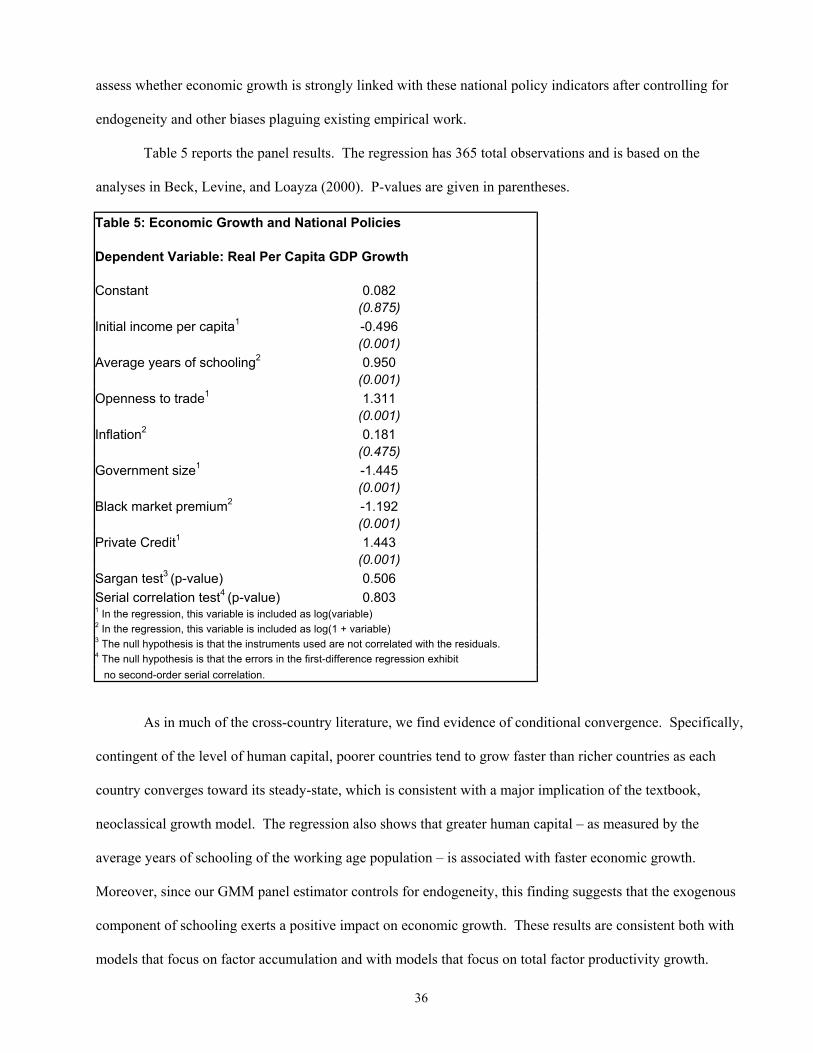
36

assess whether economic growth is strongly linked with these national policy indicators after controlling for

endogeneity and other biases plaguing existing empirical work.

Table 5 reports the panel results. The regression has 365 total observations and is based on the

analyses in Beck, Levine, and Loayza (2000). P-values are given in parentheses.

Table 5: Economic Growth and National Policies Dependent Variable: Real Per Capita GDP Growth Constant 0.082

(0.875) Initial income per capita1 -0.496

(0.001) Average years of schooling2 0.950

(0.001) Openness to trade1 1.311

(0.001) Inflation2 0.181

(0.475) Government size1 -1.445

(0.001) Black market premium2 -1.192

(0.001) Private Credit1 1.443

(0.001) Sargan test3 (p-value) 0.506 Serial correlation test4 (p-value) 0.803 1 In the regression, this variable is included as log(variable) 2 In the regression, this variable is included as log(1 + variable) 3 The null hypothesis is that the instruments used are not correlated with the residuals. 4 The null hypothesis is that the errors in the first-difference regression exhibit no second-order serial correlation.

As in much of the cross-country literature, we find evidence of conditional convergence. Specifically,

contingent of the level of human capital, poorer countries tend to grow faster than richer countries as each

country converges toward its steady-state, which is consistent with a major implication of the textbook,

neoclassical growth model. The regression also shows that greater human capital – as measured by the

average years of schooling of the working age population – is associated with faster economic growth.

Moreover, since our GMM panel estimator controls for endogeneity, this finding suggests that the exogenous

component of schooling exerts a positive impact on economic growth. These results are consistent both with

models that focus on factor accumulation and with models that focus on total factor productivity growth.

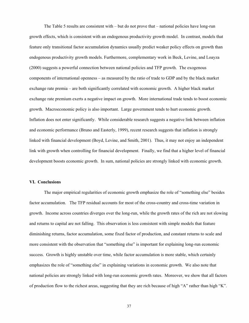
37

The Table 5 results are consistent with – but do not prove that – national policies have long-run

growth effects, which is consistent with an endogenous productivity growth model. In contrast, models that

feature only transitional factor accumulation dynamics usually predict weaker policy effects on growth than

endogenous productivity growth models. Furthermore, complementary work in Beck, Levine, and Loayza

(2000) suggests a powerful connection between national policies and TFP growth. The exogenous

components of international openness – as measured by the ratio of trade to GDP and by the black market

exchange rate premia – are both significantly correlated with economic growth. A higher black market

exchange rate premium exerts a negative impact on growth. More international trade tends to boost economic

growth. Macroeconomic policy is also important. Large government tends to hurt economic growth.

Inflation does not enter significantly. While considerable research suggests a negative link between inflation

and economic performance (Bruno and Easterly, 1999), recent research suggests that inflation is strongly

linked with financial development (Boyd, Levine, and Smith, 2001). Thus, it may not enjoy an independent

link with growth when controlling for financial development. Finally, we find that a higher level of financial

development boosts economic growth. In sum, national policies are strongly linked with economic growth.

VI. Conclusions

The major empirical regularities of economic growth emphasize the role of “something else” besides

factor accumulation. The TFP residual accounts for most of the cross-country and cross-time variation in

growth. Income across countries diverges over the long-run, while the growth rates of the rich are not slowing

and returns to capital are not falling. This observation is less consistent with simple models that feature

diminishing returns, factor accumulation, some fixed factor of production, and constant returns to scale and

more consistent with the observation that “something else” is important for explaining long-run economic

success. Growth is highly unstable over time, while factor accumulation is more stable, which certainly

emphasizes the role of “something else” in explaining variations in economic growth. We also note that

national policies are strongly linked with long-run economic growth rates. Moreover, we show that all factors

of production flow to the richest areas, suggesting that they are rich because of high “A” rather than high “K”.

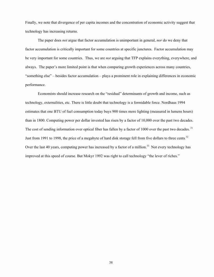
38

Finally, we note that divergence of per capita incomes and the concentration of economic activity suggest that

technology has increasing returns.

The paper does not argue that factor accumulation is unimportant in general, nor do we deny that

factor accumulation is critically important for some countries at specific junctures. Factor accumulation may

be very important for some countries. Thus, we are not arguing that TFP explains everything, everywhere, and

always. The paper’s more limited point is that when comparing growth experiences across many countries,

“something else” – besides factor accumulation – plays a prominent role in explaining differences in economic

performance.

Economists should increase research on the “residual” determinants of growth and income, such as

technology, externalities, etc. There is little doubt that technology is a formidable force. Nordhaus 1994

estimates that one BTU of fuel consumption today buys 900 times more lighting (measured in lumens hours)

than in 1800. Computing power per dollar invested has risen by a factor of 10,000 over the past two decades.

The cost of sending information over optical fiber has fallen by a factor of 1000 over the past two decades. 31

Just from 1991 to 1998, the price of a megabyte of hard disk storage fell from five dollars to three cents.32

Over the last 40 years, computing power has increased by a factor of a million.33 Not every technology has

improved at this speed of course. But Mokyr 1992 was right to call technology “the lever of riches.”

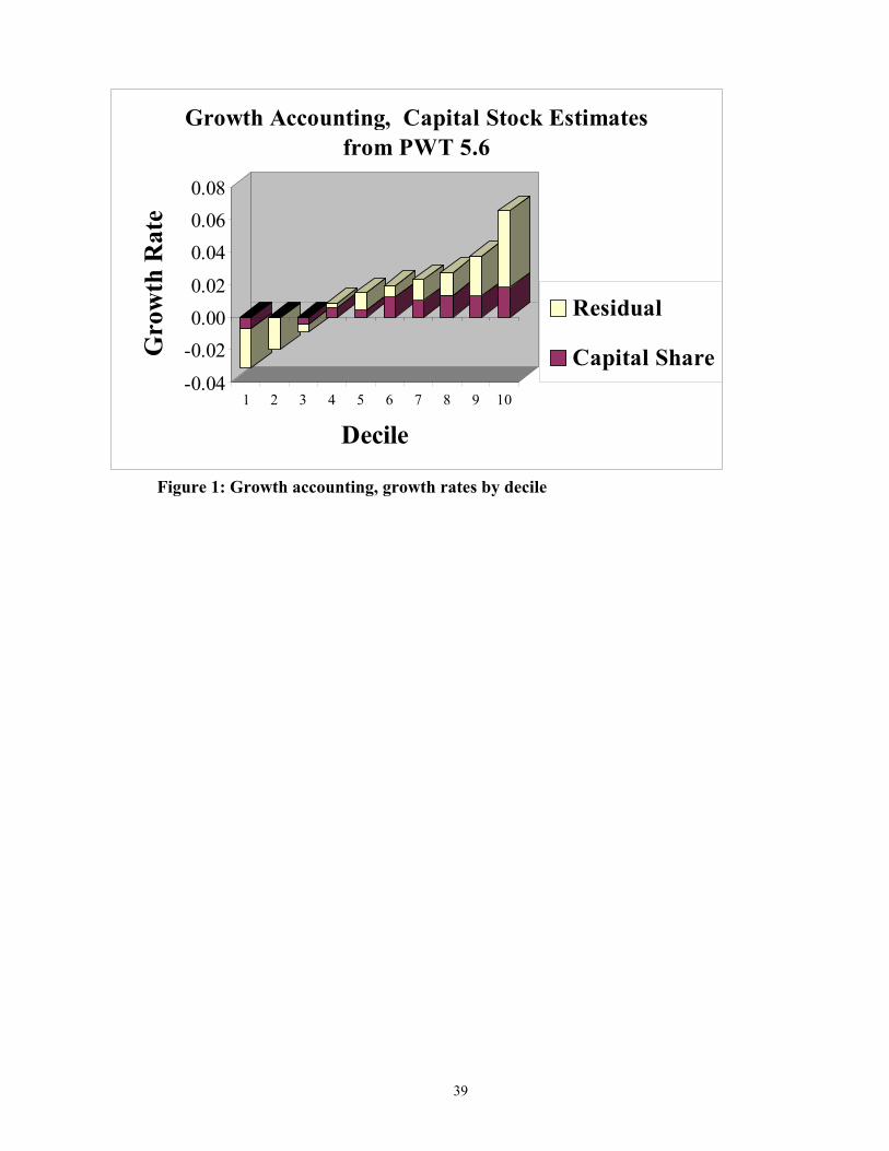
39

Figure 1: Growth accounting, growth rates by decile

-0.04

-0.020.000.02

0.040.060.08

Gro

wth

Rat

e

1 2 3 4 5 6 7 8 9 10

Decile

Growth Accounting, Capital Stock Estimates from PWT 5.6

Residual

Capital Share

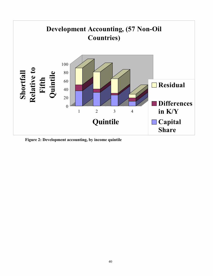
40

Figure 2: Development accounting, by income quintile

0

20

40

60

80

100

Shor

tfal

l R

elat

ive

to

Fift

h Q

uint

ile

1 2 3 4

Quintile

Development Accounting, (57 Non-Oil Countries)

Residual

Differencesin K/YCapitalShare

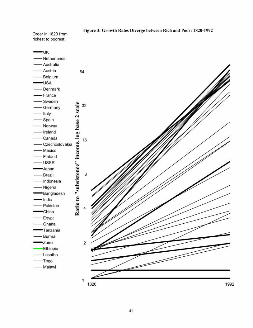
41

Figure 3: Growth Rates Diverge between Rich and Poor: 1820-1992

1820 1992

Rat

io to

"su

bsis

tenc

e" in

com

e, lo

g ba

se 2

scal

e

UKNetherlandsAustraliaAustriaBelgiumUSADenmarkFranceSwedenGermanyItalySpainNorwayIrelandCanadaCzechoslovakiaMexicoFinlandUSSRJapanBrazilIndonesiaNigeriaBangladeshIndiaPakistanChinaEgyptGhanaTanzaniaBurmaZaireEthiopiaLesothoTogoMalawi

2

4

8

16

32

64

1

Order in 1820 from richest to poorest:

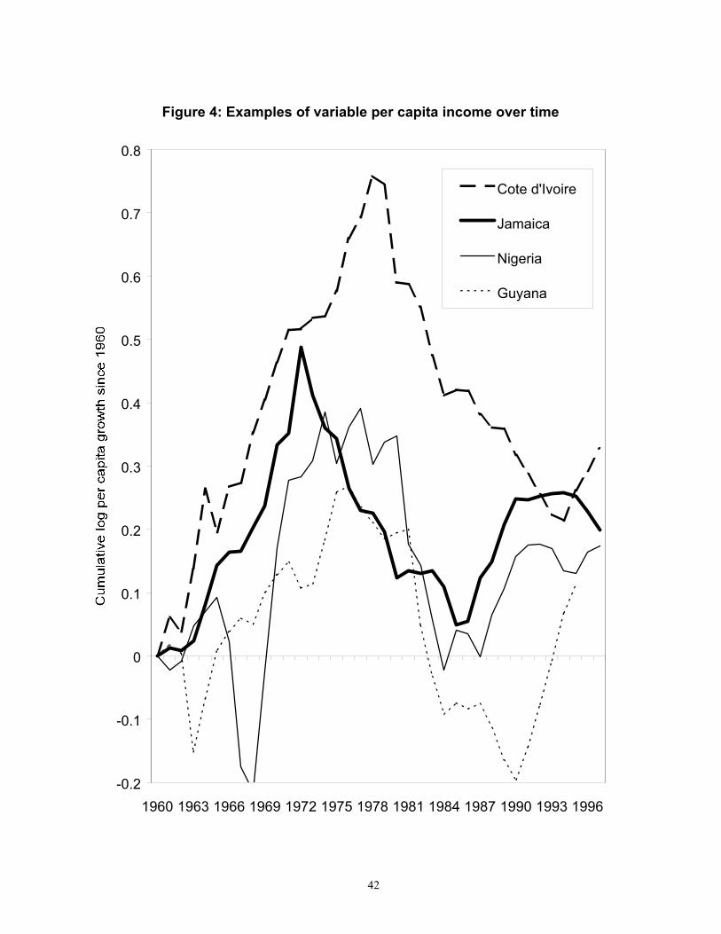
42

Figure 4: Examples of variable per capita income over time

-0.2

-0.1

0

0.1

0.2

0.3

0.4

0.5

0.6

0.7

0.8

1960 1963 1966 1969 1972 1975 1978 1981 1984 1987 1990 1993 1996

Cote d'Ivoire

Jamaica

Nigeria

Guyana

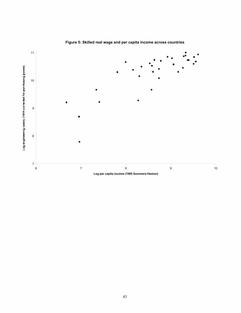
43

Figure 5: Skilled real wage and per capita income across countries

7

8

9

10

11

6 7 8 9 10

Log per capita income (1985 Summers-Heston)

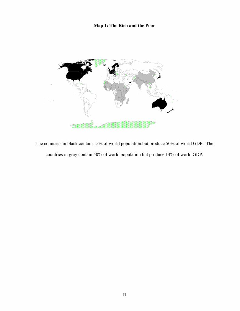
44

Map 1: The Rich and the Poor

The countries in black contain 15% of world population but produce 50% of world GDP. The

countries in gray contain 50% of world population but produce 14% of world GDP.

�� � ��

�� ������������

������ ��

������������

����������������������

����� ���

�������

�

�

��

����������� ��������� ������������

�������

������� ��� �� �

�����

������������������������������������������������������������������������������������������������������������������������������������������������������������������������������������������������������������������������������������������������������������������������������������������������������������������������������������������������������������������

���

������

�� �

������

�� ��� �� � ������

���������������

���� ��������

���������� �������� ��������

���������������������������������������������������������������

��

������

�����

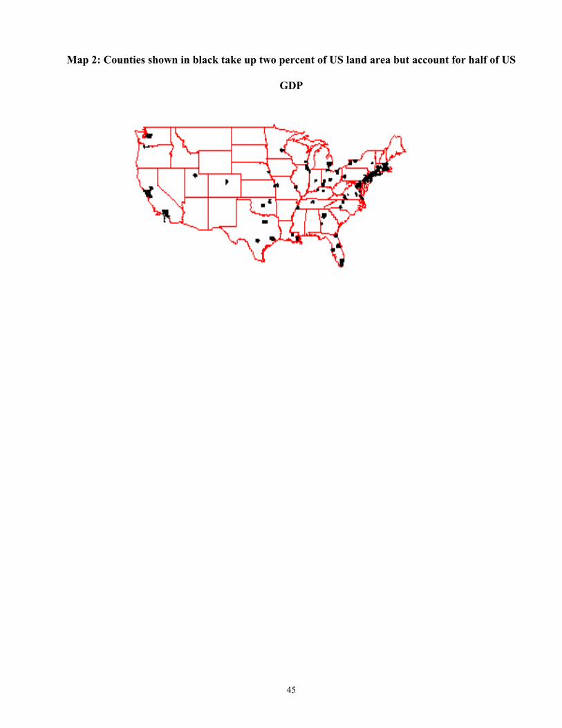
45

Map 2: Counties shown in black take up two percent of US land area but account for half of US

GDP

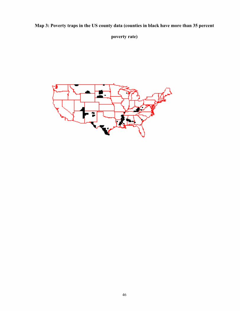
46

Map 3: Poverty traps in the US county data (counties in black have more than 35 percent

poverty rate)

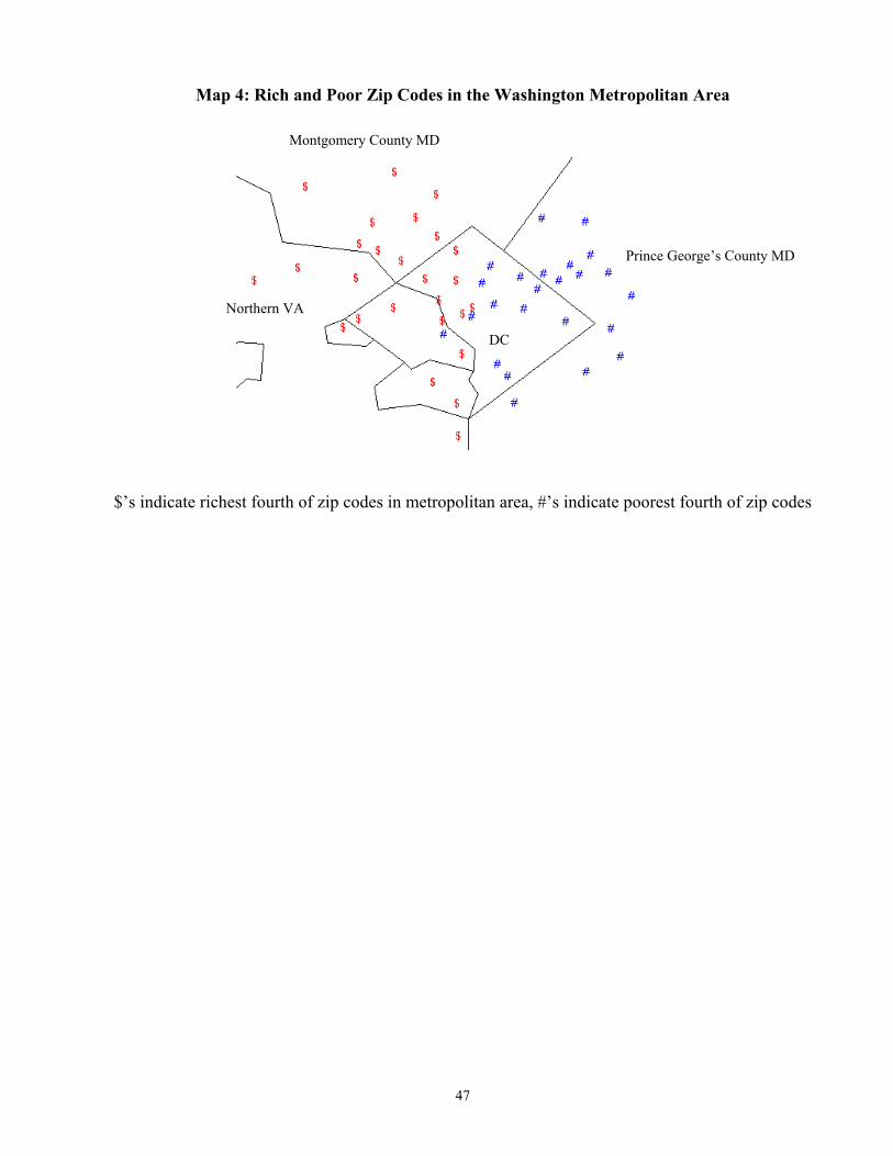
47

Map 4: Rich and Poor Zip Codes in the Washington Metropolitan Area

$’s indicate richest fourth of zip codes in metropolitan area, #’s indicate poorest fourth of zip codes

DC

Montgomery County MD

Prince George’s County MD

Northern VA

48

References

Abramovitz, M. (1956). “Resource and Output Trends in the United States since 1870,” American Economic Review, Papers and Proceedings, 46: 5-23.

Ades, Alberto and Edward Glaeser, “Evidence on growth, increasing returns, and the extent of the market,” Quarterly

Journal of Economics, Volume CXIV (3), August 1999, pp. 1025-1046. Aghion, P. and P. Howitt. Endogenous Growth Theory. MIT Press 1998. Alesina, Alberto, Reza Baqir, and William Easterly (1999) “Public goods and ethnic divisions,” Quarterly Journal of

Economics, November. Alonso-Borrego, C. and Arellano, Manuel. “Symmetrically Normalised Instrumental Variable Estimation Using Panel

Data,” CEMFI Working Paper No. 9612, September 1996. Arellano, Manuel and Bond, Stephen. “Some Tests of Specification for Panel Data: Monte Carlo Evidence and an

Application to Employment Equations,” Review of Economic Studies 1991, 58(2), pp. 277-297. Arellano, Manuel, and Bover, Olympia. “Another look at the Instrumental-Variable Estimation of Error-Components

Models,” Journal of Econometrics 1995, 68(1), pp. 29-52. Azariadis, Costas, and Allan Drazen (1990). “Threshold Externalities in Economic Development,” Quarterly Journal Of

Economics, 105:501-26 May. Baldwin, Richard E. (1998). “Global Income Divergence, Trade and Industrialization: The Geography of Growth Take-

offs,” National Bureau Of Economic Research Working Paper Series No. 6458:1-[45], March. Barro, Robert and Xavier Sala-i-Martin (1995). Economic Growth, New York: McGraw-Hill, 1995. Barro, Robert and Xavier Sala-i-Martin (1992). “Convergence,” Journal of Political Economy. Barro, Robert, J. Mankiw, N. Gregory, and X. Sala-i-Martin (1995). “Capital Mobility in Neoclassical Models of

Growth,” American Economic Review, 85:103-15 March. Basu, Susanto and John Fernald (1997). “Returns to Scale in U.S. Production: Estimates and Implications,” Journal Of

Political Economy, 105:249-83, April. Baumol, William J., “Productivity Growth, Convergence, and Welfare: What the Long Run Data Show,” American

Economic Review, December 1986, Vol. 76, No. 5, pp. 1072-1085 Beck, Thorsten; Levine, Ross; Loayza, Norman. “Finance and the Sources of Growth,” Journal of Financial Economics,

October/November 2000, 58(1-2), 261-300. Becker, Gary S., Kevin M. Murphy, and Robert Tamura (1990). “Human Capital, Fertility, and Economic Growth,”

Journal of Political Economy, Vol. 98, Number 5, Part 2, S12-S37, October. Bénabou, Roland (1996). “Heterogeneity, Stratification, and Growth: Macroeconomic Implications of Community

Structure and School Finance,” American Economic Review, 86, No. 3:584-609, June. Benabou, Roland (1993). “Workings of a City: Location, Education, and Production,” Quarterly Journal Of Economics,

108:619-52 August. Benhabib, J. and M. Spiegel (1994). “Role of Human Capital in Economic Development: Evidence from Aggregate

Cross-Country Data,” Journal of Monetary Economics, 34: 143-73.

49

Bils, Mark and P. Klenow (1996). “Does Schooling Cause Growth?,” American Economic Review, December 2000, 90(5), pp. 1160-1183.

Blomstrom, Magnus, R. Lipsey and M. Zejan (1996). “Is Fixed Investment the Key to Economic Growth?” Quarterly

Journal of Economics, February, 269-276. Blundell, Richard and Bond, Stephen. “Initial Conditions and Moment Restrictions in Dynamic Panel Data Models,”

University College London Discussion Paper 97-07, 1997. Borjas, George J. (1999). Heaven’s Door: Immigration Policy and the American Economy, Princeton: Princeton

University Press, 1999. Borjas, George J. (1995). “Ethnicity, Neighborhoods, and Human Capital Externalities,” American Economic Review, 85,

No. 3:365-90 June. Borjas, George J. (1992). “Ethnic Capital and Intergenerational Mobility,” Quarterly Journal of Economics, 107: [123]-

50 February. Borjas, George J., Stephen G. Bronars, and Stephen J. Trejo (1992). “Self Selection and Internal Migration in the United

States,” Journal of Urban Economics, No. 32, pp. 159-85, September. Bosworth, B. and S. Collins (1996). “Economic Growth in East Asia: Accumulation versus Assimilation,” Brookings

Papers on Economic Activity, No. 2: 135-203. Bouillon, César, Arianna Legovini and Nora Lustig RISING INEQUALITY IN MEXICO: RETURNS TO

HOUSEHOLD CHARACTERISTICS AND THE "CHIAPAS EFFECT", Inter-American Development Bank Mimeo, 1999

Boyd, John H.; Levine Ross; Smith, Bruce D. (2001) “The Impact of Inflation on Financial Sector Performance,” University

of Minnesota, Journal of Monetary Economics (forthcoming). Brookings Institution Center on Urban and Metropolitan Policy, A Region Divided: The State of Growth in Greater

Washington, Washington DC, 1999. Bruno, Michael, and Easterly, William. “Inflation Crises and Long-run Growth,” Journal of Monetary Economics 1998, 41,

pp. 3-26. Burnside, Craig (1996). “Production Function Regressions, Returns to Scale and Externalities,” Journal of Monetary

Economics, 37: 177-200. Carrington, William J. and Enrica Detragiache (1998). “How Big is the Brain Drain?” International Monetary Fund

Working Paper 98/102, July. Carroll, C.D. and D.N. Weil (1993). “Saving and Growth: A Reinterpretation,” Carnegie-Rochester Series on Public

Policy. Chari, V.V., L. Christiano, and E. McGrattan (1996). “The Poverty of Nations: A Quantitative Exploration,” NBER

Working Paper No. 5414. Ciccone, Antonio and Robert E. Hall (1996). “Productivity and the Density of Economic Activity,” American Economic

Review, Vol 86, No. 1, March, pp. 54-70. Collier, Paul, David Dollar, and Nicholas Stern (2000). "Fifty Years of Development," World Bank mimeo. Costello, Donna M. “Cross-country, cross-industry comparison of productivity growth.” JOURNAL OF POLITICAL

ECONOMY 101:207-22 April 1993

50

De Long, J. Bradford. “Productivity Growth, Convergence, and Welfare: Comment”, American Economic Review, December 1988, Vol. 78 No. 5, 1138-1154.

De Long, J. Bradford and Lawrence Summers. (1993) “How Strongly Do Developing Economies Benefit from

Equipment Investment?” Journal of Monetary Economics, 32: 395-416. Denison, Edward F. (1962). Sources of Economic Growth in the United States and the Alternatives Before Us, New

York: Committee for Economic Development. Denison, Edward F. (1967). Why Growth Rates Differ, Washington, DC: The Brookings Institution. Dougherty, Christopher (1991) A Comparison of Productivity and Economic Growth in the G-7 Countries, Ph. D.

Dissertation, Harvard University Easterly, William (2001), "The Lost Decades: Developing Countries' Stagnation in Spite of Policy Reform 1980-98,"

forthcoming, Journal of Economic Growth. Easterly, William (1999a) “Life During Growth,” Journal of Economic Growth, September. Easterly, William. (1999b) “The Ghost of Financing Gap: Evaluating the Growth Model of the International Financial

Institutions,” Journal of Development Economics, December. Easterly, William, Michael Kremer, Lant Pritchett, and Lawrence Summers (1993). “Good Policy or Good Luck?

Country Growth Performance and Temporary Shocks.” Journal Of Monetary Economics 32:459-83, December. Easterly, William and Sergio Rebelo. (1993), “Fiscal Policy and Economic Growth: An Empirical Investigation,” Journal

of Monetary Economics, 32: 417-458. Elias, Victor J. (1990). Sources of Growth: A Study of Seven Latin American Economies, CA: International Center for

Economic Growth. Fabricant, S. (1954). “Economic Progress and Economic Change,” 34th Annual Report of the National Bureau of

Economic Research, New York: NBER. Fischer, Stanley (1993), “The Role of Macroeconomic Factors in Growth.” Journal of Monetary Economics, 32: 485-

512. Frankel, J.A. and Romer, David “Does Trade Cause Growth?” American Economic Review, 1999, 89, pp. 379-399. Fujita, Masahisa, Krugman, Paul and Anthony Venables (1999). The Spatial Economy: Cities, Regions, and International

Trade. Griliches, Zvi (1988). “Productivity Puzzles and R&D: Another Nonexplanation,” Journal of Economic Perspectives, 2:

43-61. Grossman, G. and E. Helpman (1991). “Quality Ladders in the Theory of Economic Growth,” Review of Economic

Studies, 58: 43-61. Grubel, Herbert G., and Anthony Scott (1977). The Brain Drain: Determinants, Measurement and Welfare Effects.

Wilfrid Laurier University Press: Waterloo, Ontario, Canada. Hall, Robert E. and Charles Jones (1999). “Why Do Some Countries Produce So Much More Output per Worker than

Others?” Quarterly Journal of Economics; v114 n1 February, pp. 83-116 Hansen, Gary D. and Edward Prescott (1998). “Malthus to Solow.” National Bureau Of Economic Research. Working

Paper Series No. 6858:1-24, December.

51

Hanushek, Eric A. and Dennis D. Kimko. (2000). “Schooling, Labor-Force Quality, and the Growth of Nations,” American Economic Review, 90(5), pp. 1184-1208.

Harberger, Arnold C. (1998) “A Vision of the Growth Process,” American Economic Review, March, 88(1), pp. 1-32. Harberger, Arnold C. (1978). “Perspectives on Capital and Technology in Less Developed Countries,” in M.J. Artis and

A.R. Nobay, eds Contemporary Economic Analysis, London: Croom Helm. Holmes, T. and J.A. Schmitz, Jr. (1995). “Resistance to New Technologies and Trade between Areas,” Federal Reserve

Bank of Minneapolis Quarterly Review, 19: 2-18. Hsieh, Chang-tai (1998). “What Explains the Industrial Revolution in East Asia? Evidence from Factor Markets”

Princeton University Woodrow Wilson School Of Public And International Affairs Discussion Papers In Economics No. 196:1-42, January.

Jalan, Jyotsna and Martin Ravallion (1997). “Spatial Poverty Traps?” World Bank Policy Research Working Paper No.

1862. Jones, Chad. (1995a) “R&D-Based Models of Economic Growth,” Journal of Political Economy, August, 103, pp. 759-

84. Jones, Charles. (1995b) “Time Series Tests of Endogenous Growth Models,” Quarterly Journal of Economics, May,

105(2), 495-526. Jones, Charles. (1999). “Was an Industrial Revolution Inevitable? Economic Growth Over the Very Long Run” mimeo,

Stanford University. Jones, Charles (1997). Comment on Peter Klenow and Andres Rodriguez-Clare, “The Neoclassical Revival in Growth

Economics: Has It Gone Too Far?” NBER Macroeconomics Annual 1997, Volume 12, 73-103. Jorgenson, Dale W. (1995). Productivity, Cambridge, MA: MIT Press. Jorgenson, Dale W. and Z. Griliches (1967). “The Explanation of Productivity Change,” Review of Economic Studies, 34:

249-83. King, Robert G. and Ross Levine (1994) “Capital Fundamentalism, Economic Development and Economic Growth,”

Carnegie-Rochester Conference Series on Public Policy, 40: 259-292. King, Robert G. and Sergio Rebelo (1993). “Transitional Dynamics and Economic Growth in the Neoclassical Model,”

American Economic Review, 83: 908-31. Klenow, Peter (1998). “Ideas versus Rival Human Capital: Industry Evidence on Growth Models,” Journal of Monetary

Economics, 42: 2-23. Klenow, Peter and Andres Rodriguez-Clare (1997a). “Economic Growth: A Review Essay,” Journal of Monetary

Economics, 40: 597-617. Klenow, Peter and Andres Rodriguez-Clare (1997b). “The Neoclassical Revival in Growth Economics: Has It Gone Too

Far?” NBER Macroeconomics Annual 1997, Volume 12, 73-103. Klitgaard, Robert and Amand Fitschen (1997). “Exploring Income Variations across Traditional Authorities in KwaZulu-

Natal, South Africa,” Development Southern Africa, Vol. 14, No. 3, October. Kongsamut, Piyabha, Sergio Rebelo, Danyang Xie (1997). “Beyond Balanced Growth,” University of Rochester Working

Paper.

52

Kosmin, Barry A. and Seymour P. Lachman (1993). One Nation Under God: Religion in Contemporary American Society, Harmony Books.

Kremer, Michael (1993). “O-ring Theory of Economic Development,”Quarterly Journal Of Economics, 108:551-75

August. Krueger, Alan B. and Mikael Lindahl “Education for growth in Sweden and the world.” NATIONAL BUREAU OF

ECONOMIC RESEARCH. WORKING PAPER SERIES No. 7190:1-54, June 1999. Krugman, Paul (1998). “Space: The Final Frontier.” Journal Of Economic Perspectives, 12:161-74, Spring 1998 Krugman, Paul (1995). Development, Geography, and Economic Theory, Cambridge, MA: MIT Press. Krugman, Paul R. (1991). Geography and Trade, Cambridge MA: MIT Press. Krugman, Paul R and Anthony J.Venables (1995). “Globalization and the Inequality of Nations” Quarterly Journal of

Economics, November, pp. 857-80. Lipset, Seymour Martin (1997). American Exceptionalism: A Double Edged Sword. New York: Norton. Levine, Ross; Loayza, Norman; Beck, Thorsten. “Financial Intermediation and Growth: Causality and Causes,” Journal

of Monetary Economics, August 2000, 46, 31-77. Levine, Ross and David Renelt (1992), "A Sensitivity Analysis of Cross-Country Growth Regressions," American

Economic Review, September, 82(4), pp. 942-63. Lewis, W.A. (1954). “Economic Development with Unlimited Supplies of Labor,” The Manchester School of Economic

and Social Studies, 22(2): 139-191. Lucas, Robert E., Jr. (1988). “On the Mechanics of Economic Development,” Journal of Monetary Economics, 22: 3-42. Lucas, Robert E., Jr. (1990). Why Doesn't Capital Flow from Rich to Poor Countries? American Economic Review,

Papers And Proceedings, 80:92-96 May. Lucas, Robert E. Jr. (1998) “The Industrial Revolution: Past and Future.” Mimeo. Maddison, Angus (1995). Monitoring the World Economy, 1820-1992, Paris : Development Centre of the Organisation

for Economic Co-operation and Development. Mankiw, N. Gregory (1995). “The Growth of Nations,” Brookings Papers on Economic Activity 1, pp. 275-326. Mankiw, N. Gregory, David Romer, David N. Weil (1992). “Contribution to the Empirics of Economic Growth,”

Quarterly Journal Of Economics, 107:[407]-37. McGrattan, Ellen R. (1998) “A defense of AK growth models.” QUARTERLY REVIEW / FEDERAL RESERVE

BANK OF MINNEAPOLIS 22:13-27, Fall McGrattan, Ellen and James Schmitz (1998). “Explaining Cross-country Income Differences,” Federal Reserve Bank of

Minneapolis, Research Department, mimeo, June. Mellinger, Andrew D., Jeffrey D. Sachs, and John L. Gallup (1999) Climate, Water Navigability, and Economic

Development, Harvard Center for International Development Working Paper No. 24 Mokyr, Joel. The Lever of Riches: Technological Creativity and Economic Progress. New York: Oxford University

Press.

53

Murphy, Kevin M., Andrei Shleifer, Robert Vishny (1989). “Industrialization and the Big Push,” Journal Of Political Economy, 97:1003-26.

Nehru, Vikram and A. Dhareshwar (1993). “A New Database on Physical Capital Stocks: Sources, Methodology, and

Results,” Revista de Análisis Económico. Nehru, Vikram, Eric Swanson, and Ashutosh Dubey (1995). “A New Database on Human Capital Stock in Developing

and Industrial Countries: Sources, Methodology, and Results,” Journal of Development Economics, 46: 379-401.

Nordhaus, William “Do Real Output and Real Wage Measures Capture Reality? The History of Lighting Suggests Not,”

Yale Cowles Foundation Discussion Paper: 1078 September 1994. Parente, Stephen (1994). “Technology Adoption, Learning-by-Doing, and Economic Growth,” Journal of Economic

Theory, 63: 346-69. Parente, S.L. and Prescott, E.C. (1996) “Barriers to Technology Adoption and Development,” Journal of Political

Economy, 102(2), pp. 298-321. Patrinos, Harry Anthony (1997). “Differences in Education and Earnings Across Ethnic Groups in Guatemala,”

Quarterly Review of Economics and Finance, 37 (4). Prescott, Edward (1998). “Needed: A Theory of Total Factor Productivity,” International Economic Review,

forthcoming. Pritchett Lant. (1999). “The Tyranny of Concepts: CUDIE (Cumulated, Depreciated, Investment Effort) is Not Capital”,

World Bank mimeo. Pritchett, Lant (1998). “Patterns Of Economic Growth : Hills, Plateaus, and Mountains,” World Bank Development

Research Group Policy Research Working paper No. 1947. Pritchett, Lant (1997). “Where Has All the Education Gone?” World Bank Policy Research Working Paper No. 1581. Psacharopoulos, George (1994). “Returns to Investment in Education: A Global Update,” World Development, Vol. 22,

No. pp. 1325-1343. Psacharopoulos, George and Harry Anthony Patrinos (1994). “Indigenous People and Poverty in Latin America,” Human

Resources Development and Operations Policy Working Paper #22. Quah, Danny. “Galton's Fallacy and Tests of the Convergence Hypothesis.” Scandinavian Journal of Economics; v95 n4

December 1993, pp. 427-43. Rauch, James E. (1993). “Productivity Gains from Geographic Concentration of Human Capital: Evidence from the

Cities,” Journal Of Urban Economics, 34:380-400. Rappaport, Jordan and Jeffrey Sachs. (1999). “The United States as a Coastal Nation.” Harvard Center for International

Development, Mimeo Ravallion, Martin and Jyotsna Jalan (1996). “Growth Divergence Due to Spatial Externalities,” Economics Letters 53,

227-232. Ravallion, Martin and Quentin Wodon (1998). “Poor Areas or Only Poor People?” mimeo World Bank. Ray, Debraj (1998). Development Economics. Princeton: Princeton University Press. Rebelo, Sergio (1991) “Long-run Policy Analysis and Long-run Growth,” Journal of Political Economy 99, 500-521.

54

Rebelo, Sergio (1998). “The Role of Knowledge and Capital in Economic Development,” Northwestern University, mimeo.

Rebelo, Sergio and Nancy L. Stokey (1995). “Growth Effects of Flat-rate Taxes,” Journal Of Political Economy,

103:519-50. Rodrik, Dani (1998). “Where Did all the Growth Go? External Shocks, Social Conflict and Growth Collapses,” National

Bureau Of Economic Research. Working Paper Series No. 6350. Romer, Paul (1995). Comment on N. Gregory Mankiw, “The Growth of Nations,” Brookings Papers on Economic

Activity 1, pp. 313-320. Romer, Paul (1990). “Endogenous Technological Change,” Journal of Political Economy, 98: S71-S102. Romer, Paul (1986). “Increasing Returns and Long-Run Growth,” Journal of Political Economy, 94: 1002-37. Rostow, W. W. (1960). The Stages of Economic Growth : A Non-Communist Manifesto, Cambridge University Press. Shleifer, Andrei and Robert Vishny (1993). “Corruption,” Quarterly Journal of Economics, 108(3): 599-667. Solow, R. (1957). “Technical Change and the Aggregate Production Function,” Review of Economics and Statistics, 39:

312-20. Solow, R. (1956). “A Contribution to the Theory of Economic Growth,” Quarterly Journal of Economics, 70: 65-94. Union Bank of Switzerland (1994). Prices and Earnings Around the Globe, Zurich. United States Government (1996). 1995 Statistical Abstract of US, Washington DC. World Bank (2000a), Can Africa Claim the 21st Century, Washington DC World Bank (2000b), The Road to Stability and Prosperity in South Eastern Europe, Europe and Central Asia Region,

Washington DC. World Bank (2000c), East Asia: Recovery and Beyond, Washington DC World Bank 2000/2001 World Development Report: Attacking Poverty. Washington DC Young, Alwyn (1995). “The Tyranny of Numbers: Confronting the Statistical Realities of the East Asian Growth

Experience,” Quarterly Journal of Economics, 110: 641-680.

55

Endnotes

1 This is a reversal and slight rewording of Arthur Lewis’s (1954, p. 155) famous quote, “The central problem in the theory of economic development is to understand the process by which a community which was previously saving and investing 4 or 5 percent of its national income or less, converts itself into an economy where voluntary saving is running at about 12 to 15 percent of national income or more. This is the central problem because the central fact of development is rapid capital accumulation (including knowledge and skills with capital).” While Arthur Lewis recognizes the importance of knowledge and skills and later in his book highlights the importance of institutions, many development economists who followed Lewis adopted the more limited focus on saving and physical capital accumulation. 2 Academic researchers in the 1990s started a "neoclassical revival" (in the words of Klenow and Rodriguez-Clare 1997). The classic works in the academic literature's stress on factor accumulation were Mankiw, Romer and Weil 1992, Barro, Mankiw, and Sala-i-Martin 1995, Mankiw 1995, and Young 1995. The summary of the Global Development Network conference in Prague in June 2000, representing many international organizations and development research institutes, says "physical capital accumulation was found to be the dominant source of growth both within and across regions. Total factor productivity growth (TFPG) was not as important as was previously believed" (http://www.gdnet.org/pdfs/GRPPragueMtgReport.pdf). A leading development textbook (Todaro 2000) says that an increase in investment is "a necessary condition" for economic takeoff. The development textbook of Ray (1998) refers to investment and saving as "the foundations of all models of economic growth." Many development practitioners also stress investment. For example, the International Monetary Fund (1996) argues, “The adjustment experience of sub-Saharan Africa has demonstrated that to achieve gains in real per capita GDP an expansion in private saving and investment is key.” The Bank for International Settlements (1996) concludes, “recent experience has underlined the central importance of national saving and investment rates in promoting growth.” And, the International Labor Organization (1995) argues that “policies to raise the rate of investment... are critical for raising the rate of growth and employment in an economy.” Finally “additional investment is the answer -- or part of the answer -- to most policy problems in the economic and social arena” (United Nations 1996). Similarly, the World Bank (1993) states that in East Asia, “accumulation of productive assets is the foundation of economic growth.” World Bank (1995) promises that in Latin America, "enhancing saving and investment by 8 percentage points of GDP would raise the annual growth figure by around 2 percentage points." World Bank 2000a says the saving rate of the typical African country "is far below what is needed to sustain a long-term boost in economic performance." The World Bank 2000b says that South Eastern Europe can only seize trade opportunities if "domestic and foreign entrepreneurs increase their investment dramatically." For more citations, wee Easterly (1997) and King and Levine (1994).Although common, the stress on capital accumulation is far from universal among development practitioners and researchers. For example, the World Bank 2000c report on East Asia's recovery suggested "future growth hinges less on increasing physical capital accumulation and more on raising the productivity growth of all factors." Collier, Dollar, and Stern 2000 stressed policies, incentives, institutions, and exogenous factors as the main drivers in growth with little mention of investment, as does the 2000/2001 World Development Report (pp. 49-52). 3 We use the summary in Barro and Sala-i-Martin (1995, p.380-1). 4 This point is due to Barro and Sala-i-Martin 1995, p. 352. 5 The paper reports results using the capital stock estimates from the Penn World Tables, version 5.6. The Penn World Tables documents the construction of this data. We also constructed capital stock figures for more countries using aggregate investment figures. For some countries, the data start in 1951. These data use real investment in 1985 prices and real GDP per capita (chain index) in constant 1985 prices. We use a perpetual inventory method to compute capital stocks. Specifically, let K(t) equal the real capital stock in period t. Let I(t) equal the real investment rate in period t. Let d equal the depreciation rate, which we assume equals 0.07. Thus, the capital accumulation equations states that K(t+1) = (1-d) K(t) + I(t). To compute the capital per worker ratio we divide K(t) by L(t), where L(t) is the working age population in period t as defined in the Penn World Tables. To compute the capital-output ratio, we divide K(t) by Y(t), where Y(t) is real GDP per capita in period t. To make an initial estimate of the capital stock, we make the assumption that the country is at its steady-state capital-output ratio. Thus, in terms of steady-state value, let k = K/Y, let g = the growth rate of real output, let i = I/Y. Then, from the capital accumulation equation plus the assumption that the country is at its steady-state, we know that k = i/[g + d]. Thus, if we can obtain reasonable estimates of the steady-state values of i, g ,and d, then we can compute a reasonable estimate of k. The Penn World Tables have data going back to 1950 on output. Thus, we can compute the initial capital stock estimate as k*Y(initial). To makes the initial estimate of k, the

56

steady state capital output ratio, we set d=0.07. We construct g – the steady-state growth rate -- as a weighted averaged of the countries average growth rate during the first ten years for which we have output and investment data and the world growth rate. The world growth rate is computed as 0.0423. Based on Easterly et al. (1993, Journal of Monetary Economics), we give a weight of 0.75 to the world growth rate and 0.25 to the country growth rate in computing an estimate of the steady-state growth rate for each individual country, g. We then compute i as the average investment rate during the first ten years for which there are data. Thus, with values for d, g, and i for each country, we can estimate k for each country. To reduce the influence of business-cycles in making the estimate of Y(initial), we use the average real output value between 1950-1952 as an estimate of initial output, Y(initial). Thus, the capital stock in 1951 is given as Y(initial)*k. If output and investment data do not start until 1960, everything is moved up one decade for that country. Given depreciation, the guess at the initial capital stock becomes relatively unimportant decades later. 6 It may be that the conventional measure of investment effort is a cost-based measure that does not translate necessarily into increasing the value of the capital stock. Pritchett 1999 makes this point, especially –but not only – with regard to public investment. 7 Again, different authors use different weights, though this tends not to change the basic findings. 8 These estimates are based on schooling and job experience. 9 While not directly related to growth accounting, note that the K/Y ratio systematically varies with income per capita. Capital-output ratios are systematically larger in richer countries; and, capital-output ratios tend to rise as countries grow, which are inconsistent with Kaldor’s stylized fact on capital-output ratios. Consider the regression of the capital-output ratio (κi ) on a measure of income per capita relative to that in the United States in the 1980s (yi/yUSA). The regression yields the following result: κi = 0.76 + 0.59[yi/yUSA], (0.10) (0.18) where κi is the capital-output ratio in country i, standard errors are in parentheses, and the regression includes 57 non-oil countries. There is a strong positive relationship between output per person relative to the United States and the K/Y ratio. Also, Figure 3 shows that the K/Y ratio tends to rise in fast growing countries. Here, we take countries that grew faster than 3.5% per year in per capita terms over the period 1960-1992. We then plot, year-by-year, the average value of their K/Y ratios. As shown, the K/Y ratio rises rapidly over this fast growth period. While these differences might be due to transitional dynamics, past works suggests that physical capital accumulation along the transition path is unlikely to explain fully level and growth differences [King and Rebelo 1993]. 10 Yet, Burnside (1996) presents evidence that suggests that physical capital externalities seem to be relatively unimportant. Also, Klenow (1998) presents evidence that is consistent with technological change based model of growth. 11 Costello (19933) shows that TFP has a strong country component and is not specific to particular industries. 12 See Holmes and Schmitz (1995), Parente (1994), Parente and Prescott (1996), and Shleifer and Vishny (1993). 13 See Lucas 1998 for an extensive discussion of this divergence, which he interprets as reflecting different takeoff times for various economies, and which he predicts will decrease as new countries “take off.” 14 The usual finding that initial income and growth are uncorrelated relied on data that went through 1981 or 1985, and did a linear regression of growth on initial income. The use of more recent data (through 1992) and the analysis of quintiles account for our finding of absolute divergence. 15 Data on per capita taken from Summers and Heston. The low persistence of growth rates, and the high persistence of investment and education, was previously noted in Easterly, Kremer, Pritchett, and Summers 1993 16 Data from Maddison 1995.

57

17 Models supposing a linear relationship between growth and investment have a long history in economics. See Easterly (1999b) for a review of the Harrod-Domar tradition that continues down to the present. For a new growth theory justification of this relationship, see McGrattan (1998). 18 37 countries had a growth drop of 5 percentage points or more, 19 countries had a growth increase of 5 percentage points or more, and 8 countries were included in both groups. 19 The non-persistence of growth rates does not inherently contradict the stylized fact of divergence or the stylized fact that national policies influence long-run growth rates. While policies are (a) persistent and (b) significantly associated with long-run growth (which is not persistent), the R-square of the growth regression is generally smaller than 0.50. Thus, something else (besides national policies) is very important for explaining cross-country differences in long-run growth rates. In terms of divergence, the non-persistence of growth rate stylized fact emphasizes that growth follows very different paths across countries and that there is a high degree of volatility. Nevertheless, there are countries that have achieved comparatively greater success over the long-run. While France, German, and England have experienced growth fluctuations, they have enjoyed a steeper – and less volatile – growth path than Argentina and Venezuela for example. Argentina, Venezuela, and other countries growth paths have not only been more volatile, they have experienced dramatic changes in trends. 20 These calculations omit the oil countries, in which GDP is not properly measured because all of oil extraction is treated as current income rather than asset depletion. 21 An alternative explanation would be that some land areas, accounting for a small share of the earth’s surface, have a large productivity advantage. Mellinger, Sachs, and Gallup 1999 argue that temperate coastal zones have a large productivity advantage. If this were true, we would expect to see economic activity distributed fairly evenly along temperate coastal zones (adjusting for any small intrinsic differences among such zones). However, even along temperate coastal zones, casual observations would suggest high bunching of activity. 22 Metropolitan counties are those that belong to a PMSA or MSA in the census classification of counties. 23 Brookings 1999 notes this East-West geographic divide of the Washington area shows up in many socioeconomic variables like poverty rates, free and reduced price school lunches, road spending, etc. 24 From the Urban Institute's Underclass Database, which contains data on white, black, and "other" population numbers for 43, 052 census tracts in the US. 25 Tables 52 and 724, 1995 Statistical Abstract of US. 26 Ethnic differentials are also common in other countries. The ethnic dimension of rich trading elites is well-known: the Lebanese in West Africa, the Indians in East Africa, and the overseas Chinese in Southeast Asia. Virtually every country has its own ethnographic group noted for their success. For example, in The Gambia a tiny indigenous ethnic group called the Serahule is reported to dominate business out of all proportion to their numbers -- they are often called “Gambian Jews.” In Zaire, Kasaians have been dominant in managerial and technical jobs since the days of colonial rule -- they are often called “the Jews of Zaire” (New York Times, 9/18/1996). 27 Ciccone and Hall 1996 have a related finding for US states. 28 The t-statistics are 8.2 for the log of population density in 1980 and 8.9 for the log of per capita income in 1979. The equation has an R-squared of .065 and 3133 observations. The county data are from Alesina, Baqir, and Easterly 1999. 29 Note these are all small countries. Carrington and Detragiache 1998 point out that US immigration quotas are less binding for small countries, since with some exceptions the legal immigration quota is 20,000 per country regardless of a country’s population size. 30 Casual observation suggests “brain drain” within countries. The best lawyers and doctors congregate within a few metropolitan areas like New York, where skilled doctors and lawyers are abundant, while poorer areas where skilled doctors and lawyers are scarce have difficulty attracting the top-drawer professionals.

58

31 World Bank, 1998/99 World Development Report, p. 3, p. 5, p. 57 32 http://www.duke.edu/~mccann/q-tech.htm#Death of Distance 33Brad de Long’s web site: http://econ161.berkeley.edu/E_Sidebars/E-conomy_figures2.html