A 2 0 - Y E A R

P L A N T O

E N A B L E

E A R T H Q U A K E

P R E D I C T I O N

GESSG L O B A L . E A R T H Q U A K E . S A T E L L I T E . S Y S T E M

M A R C H 2 0 0 3

Executive Summary

Earthquake Hazard Assessmentin the Future

Scientific Motivation

Enhanced Low-Earth Orbit

Geosynchronous Architecture

Optimizing the Measurement

Technology Studies

The 20-Year Plan

Appendix

2

14

28

50

66

4

76

95

CONTENTST A B L E . O F

98

C H A P T E R

O N E

C H A P T E R

T W O

C H A P T E R

T H R E E

C H A P T E R

F O U R

C H A P T E R

F I V E

C H A P T E R

F I V E

H E E L E G A N C E O F T H E T H E O R Y O F

plate tectonics, and the predictability of plate motions,

led to an optimistic view during the 1970s that individual

earthquakes could be predicted. Decades later, the real-

ization that the dynamics of the solid Earth are complex,

nonlinear, and self-organizing has somewhat dampened

the early optimism for predicting earthquakes, but has

also stimulated a vigorous effort to model and under-

stand their complexity. Today, the importance of a predic-

tive capability can hardly be overstated, as populations

in seismically active areas continue to grow, and potential

economic losses widen. What will it take to predict

earthquakes?

The advent of space geodesy — the science of measuring

deformation of the solid Earth — has enabled major

advances in understanding the deforming crust. Global

Positioning System (GPS) geodesy, and recently the

European Remote Sensing (ERS) synthetic aperture radar

(SAR) satellites, have given us a glimpse of the revolution

in understanding that will come with systematic, highly

accurate observations of surface deformation. The near-

term prospect of predicting a certain magnitude earth-

quake on a specific fault, occurring on a particular day

or week, is expected to remain out of reach. However,

dynamic hazard assessments of individual fault systems

at time scales of months appear to be feasible if frequent,

high-precision deformation measurements are available.

The NASA Solid Earth Science Working Group (SESWG)

produced a report, “Living on a Restless Earth,” that

offers as its first priority the need for a highly capable

system for measuring global surface deformation for

understanding earthquakes, as well as myriad other geo-

physical phenomena. This study translates that recom-

mendation into a detailed implementation plan, focused

specifically on improving understanding of earthquakes.

To initiate our study of a Global Earthquake Satellite Sys-

tem (GESS) that could provide the data needed to enable

prediction, we gathered from the scientific community

measurement requirements to address outstanding

problems. These requirements were combined with the

needs of the disaster response community, and drove

the definition of a plan for an end-to-end program that

would enable earthquake forecasting.

Although there are diverse geophysical phenomena —

electromagnetic and thermal emissions in particular —

that appear to bear some relationship to the earthquake

cycle, only surface deformation and seismicity can be

directly related to it. We focused the observational

scenario on obtaining synoptic measurements of surface

deformation at appropriate accuracies and temporal

scales to reveal the behavior of the crust as it accumu-

lates strain between earthquakes and relieves it through

coseismic ruptures, aseismic slip, and other transient

T

Executive Summary

2

deformation. The optimal system for measuring charac-

teristic surface deformation is an L-band interferometric

SAR (InSAR) because the wavelength favors long-term

correlation, the measurement capability is all-weather,

and the technique allows for automated, wide-area map-

ping. Our mission and technology studies have, therefore,

focused on InSAR missions, and specifically, constellations

in different orbit configurations. The required number of

satellites decreases with altitude, so a constellation of

several satellites in geosynchronous orbit (GEO) performs

as well as many more satellites in low-Earth orbit (LEO).

We develop detailed mission architectures for an en-

hanced LEO constellation, as well as a GEO constellation.

To advance towards a reliable predictive capability

requires that deformation must be resolved at an abso-

lute accuracy of approximately 1 mm/yr over the course

of a decade.

The future modeling environment will maximize the

impact of InSAR data by folding current observations into

system models. The observational data, including InSAR,

GPS, seismicity, and strainmeters, will be assimilated into

computational models, which will evolve as they are con-

strained and verified by the data. The physical processes

associated with solid-Earth deformation interact over

many spatial and temporal scales. Recent work suggests

strong correlations in both space and time, resulting in

observable space–time patterns. Data mining will be

needed for analyzing the terabytes per day of streaming

data in order to search for anomalies and recognize the

emerging behavior of interacting fault systems. Near-line

and online archives, and rapid access, are critical to en-

able continuous examination of system behavior, and to

provide appropriate and timely data and information to

the United States Geological Survey, Federal Emergency

Management Agency, the California Office of Emergency

Services, and others.

The disaster management community generally needs

information as soon as possible. Their needs drive the

data latency requirement, as well as the spatial resolu-

tion. Decorrelation is a strong indication of collapsed

structures, and the ability to map damaged neighbor-

hoods, for example, within hours of an earthquake would

be a great benefit. Data are needed within 24 hours and

preferably within two hours for maximum effectiveness.

The challenging observational program described in

the report naturally results in a list of investments

needed to accelerate development of technology com-

ponents. At the top of this list are large (30 m diameter),

lightweight, low-cost, active, electronically steerable

antennas; lightweight, low-power radar electronics; and

development of new processing systems for high-van-

tage-point observations. Models must be developed to

estimate the tropospheric water vapor along the radar

line-of-sight. And in order to maximize societal benefits,

we must invest in creating the ability to merge data sets,

rapidly analyze them, and inform interested parties of an

impending earthquake.

The measurement requirements generated by the scien-

tific community and the technology roadmaps for differ-

ent architectures lay the groundwork for building a truly

comprehensive global earthquake satellite system. The

first step is to focus on surface deformation measure-

ments through progressively advanced L-band InSAR

systems and aggressive modeling. These studies, pre-

sented here, constitute important steps towards under-

standing earthquake physics well enough to forecast

earthquakes and save lives and assets.

3SUMMARYE X E C U T I V E S U M M A R Y

G L O B A L . E A R T H Q U A K E . S A T E L L I T E . S Y S T E M4

C H A P T E R

O N E

nderstanding the earthquake cycle and assessing earthquake hazards is a

topic of both increasing potential for scientific advancement and societal

urgency. A large portion of the world’s population inhabits seismically active

regions, including the megacities of Los Angeles, Tokyo, and Mexico City, and

heavily populated regions in Asia. Furthermore, the recent devastating Gujurat

earthquake in India and the New Madrid series of earthquakes in the U.S.

underscore the vulnerability of areas not thought to be tectonically active.

Population growth will exacerbate the potential for huge earthquake-related

casualties, and economic losses of tens of billions of dollars will likely occur as a

result of future large events. Since earthquake losses, human and material, are

primarily the result of structural failures, enforcing appropriate building codes

and retrofitting structures can reduce the overall hazard.

Knowledge of the overall earthquake hazard, and more specific regional and

local earthquake risk (at the scale of fault systems) is needed to effectively

mitigate these earthquake hazards. A global earthquake observing system will

monitor the behavior of interacting fault systems, identify unknown (subsurface)

faults, guide new models of the deforming crust, and verify those dynamic

models. This knowledge will translate into tangible societal benefits by providing

the basis for more effective hazard assessments and mitigation efforts.

U

Inset and background: Effects of the Northridge, California, earthquake. (Robert Eplett, CA OES)

Earthquake Hazard Assessment in the Future

5

During the last decades, powerful new tools

to observe tectonic deformation have been de-

veloped and deployed with encouraging results

for improving knowledge of fault system behav-

ior and earthquake hazards. In the future, the

coupling of complex numerical models and or-

ders of magnitude increase in observing power

promises to lead to accurate, targeted, short-

term earthquake forecasting. Dynamic earth-

quake hazard assessments resolved for a range

of spatial scales (large and small fault systems)

and time scales (months to decades) will allow

a more systematic approach to prioritizing the

retrofitting of vulnerable structures, relocating

populations at risk, protecting lifelines, prepar-

ing for disasters, and educating the public.

The suite of spaceborne observations needed

to achieve this vision has been studied, and

the derived requirements have defined a set

of mission architectures and enabling tech-

nologies that will accelerate progress in achiev-

ing the goal of improved earthquake hazard

assessments.

Three decades ago, earthquake prediction

was thought to be an achievable goal. Such op-

timism has all but vanished in the face of cur-

rent understanding of the complexity of the

physics of earthquake fault systems. The advent

of dense geodetic networks in seismically active

regions (e.g., SCIGN, the Southern California

Integrated Global Positioning System Net-

work), and satellite interferometric synthetic

aperture radar (InSAR) from the European Re-

mote Sensing (ERS) satellites, have resulted in

great progress in understanding fault ruptures,

transient stress fields, and the collective behav-

ior of fault systems, including transfer of

stresses to neighboring faults following earth-

quakes (Freed and Lin, 2001; Pollitz and Sacks,

2002). These improved observations of surface

deformation, coupled with advances in compu-

tational models and resources, have stimulated

numerical simulations of fault systems that at-

tempt to reveal system behavior. As InSAR

and Global Positioning System (GPS) data be-

come more spatially and temporally continuous

in the future, the modeling environment will

rapidly evolve to achieve revolutionary ad-

vances in understanding the emergent behavior

of fault systems. This in turn will enable finer

temporal resolution (dynamic) earthquake haz-

ard assessments on the scale of individual faults

and fault systems. Dynamic earthquake hazard

assessment, coupled with rapid postearthquake

damage assessments will enable more effective

management of seismic disasters.

The Global Earthquake Satellite System

(GESS) study began with the requirements

generated for the LightSAR mission, as well as

those generated in an EarthScope workshop

focused on InSAR ( J. B. Minster, personal

communication, 2001). EarthScope is a Na-

tional Science Foundation (NSF) initiative,

carried out in partnership with the United

States Geological Survey (USGS) and NASA,

to study crustal deformation in North America.

NASA’s proposed contribution to the initiative

is an InSAR satellite. Under EarthScope,

NSF will field an array of approximately 1000

GPS monitoring sites across western North

America, one or more strainmeters, and several

deep drill holes near the San Andreas fault.

The USGS will upgrade and expand its digital

seismic network as its contribution. The syner-

gistic combination of these measurements and

InSAR-observed surface deformation is ex-

pected to yield major advances in understand-

ing of the crustal structure and rheology of the

continent.

Whereas the requirements for a near-term

InSAR satellite are well understood, the future

needs, which are not well defined, are the

driver for our study. Therefore, we have exam-

HAZARDSE A R T H Q U A K E . H A Z A R D . A S S E S S M E N T

G L O B A L . E A R T H Q U A K E . S A T E L L I T E . S Y S T E M6

ined the outstanding questions concerning the

physics and forecasting of earthquakes, and

used these as the basis of a Request for Propos-

als, issued by JPL, to fund studies that defined

measurement requirements for an observing

system that could answer them. These ques-

tions are:

1. How does the crust deform during the

interseismic period between earthquakes

and what are its temporal characteristics

(if any) before major earthquakes?

2. How do earthquake ruptures evolve both

kinematically and dynamically and what

controls the earthquake size?

3. What controls the space–time characteristics

of complex earthquakes and triggered

earthquakes and aftershocks?

4. What are the sources and temporal charac-

teristics of postseismic processes and how

does this process relate to triggered seismicity?

5. How can we identify and map earthquake

effects postseismically or identify regions

with a high susceptibility to amplified ground

shaking or liquefaction/ground failure?

6. Are there precursory phenomena (potential

field, electromagnetic effects, or thermal

field changes) preceding earthquakes that

could be resolved from space?

Incorporating this community input, we

have formulated a more stringent set of re-

quirements for measurement of surface defor-

mation that will answer questions 1–4, and we

consider approaches to addressing questions

5 and 6. The drivers for these requirements

are discussed below and in Chapter 2.

Elements of a Global EarthquakeS atellite Obser ving System

Efforts to advance understanding of earth-

quake physics require detailed observations of

all phases of the earthquake cycle (pre-, co-,

and postseismic), across multiple fault systems

and tectonic environments, with global distri-

bution. Satellites offer the best way to achieve

global coverage and consistent observations of

the land surface. While ground seismometer

and GPS networks are and will remain critical,

the synoptic view of the deforming crust that is

possible using satellite data drives the need for

a global earthquake satellite observing system.

In addition, knowledge of the character of

the shallow subsurface is critical to assessing

expected ground accelerations.

S u r f a c e D e f o r m a t i o n M e a s u r e m e n t s

Measurement of surface change (displace-

ment) constitutes a powerful tool for resolving

the deformation fields resulting from tectonic

strain (Figure 1.1). Surface deformation in-

cludes other components besides tectonic

strain, such as surface motion due to ground-

water storage and retrieval (Bawden et al.,

2001). The InSAR technique relies on corre-

lated image-pairs to derive displacements to

the resolution of a fraction of the radar wave-

length. If topography is known, two images

can be used to derive a map of the displace-

ment in the range direction. Additional image

pairs obtained from different look directions

(i.e., ascending versus descending) improve

the resolution of vertical and horizontal dis-

placements. If topography is not known, three

images can be differenced to derive the topog-

raphy and its change. The accuracy of the mea-

surement depends on several factors, including

the radar signal-to-noise ratio (SNR), orbit

determination precision, and removal of signal

path delays caused by the variations in spurious

ionospheric electron density and tropospheric

water vapor. All of these errors must be mini-

mized to achieve long-term absolute accuracy

of interseismic strain accumulation.

7

S u b s u r f a c e C h a r a c te r i s t i c s

The type of material in the shallow subsur-

face, and its saturation, affect the ground

acceleration experienced as a result of a par-

ticular earthquake. Directivity of seismic

energy during fault rupture can result in quite

different patterns of deformation. Liquefac-

tion, the sudden release of water from

saturated, permeable layers, is of particular

concern in coastal landfill areas, and on steep

slopes. Mapping the degree of saturation in

the shallow subsurface will help determine

landslide hazards, and may allow the liquefac-

tion hazard to be folded into the overall dy-

namic earthquake hazard assessment. Radar

sounders, along with InSAR displacements,

can provide data to augment surface measure-

ments that seek to characterize the subsurface.

E l e c t r o m a g n e t i c a n d T h e r m a l A n o m a l yP r e c u r s o r s

Many claims have been made concerning

the correlation of magnetic fields, electric

fields, and seismicity, including precursory

electromagnetic signals. Mechanisms to pro-

duce such correlative variations include move-

ment of fluids in fault zones as a result of

stress changes preceding ruptures, and

piezomagnetic effects of stress field changes.

Improvements in data quality and quantity

over the past 40 years have led to a substantial

decrease in the correlated signals ( Johnston,

1997). Magnetic anomalies associated with

main shocks are well documented and can be

accounted for by piezomagnetic effects. The

subject of precursory electromagnetic signals,

and a satisfactory mechanism to explain them,

requires more laboratory and field research, as

well as high-quality continuous ground and

satellite magnetic field data series with proper

reference control. Recognizing subtle signals

generated at the surface against the back-

ground of the highly dynamic external mag-

netic field at satellite altitudes is challenging.

These correlations are likely best tested using

carefully configured ground networks in

seismogenic zones.

A weak infrared (IR) thermal anomaly was

observed near the epicenter of the October

1999 Hector Mine, California, earthquake

(Figure 1.2). This and other suggested corre-

lations between thermal IR anomalies and

Figure 1.1

Earthquakes can

cause significant

surface deformation,

such as this meter

offset from an

earthquake in the

California desert.

(Robert Eplett,

CA OES)

HAZARDSE A R T H Q U A K E . H A Z A R D . A S S E S S M E N T

G L O B A L . E A R T H Q U A K E . S A T E L L I T E . S Y S T E M8

earthquakes have been studied with inconclu-

sive results. As with electromagnetic anomalies,

more robust correlations and plausible mecha-

nisms are needed to assess this potential stress

indicator. The current Advanced Spaceborne

Thermal Emission Radiometer (ASTER) and

Landsat ETM+ instruments have good spatial

resolution, and may provide data to test exist-

ing hypotheses, but coverage is sparse.

Spatial and Temporal MeasurementRequirements

The primary focus of the GESS study

was the measurement of surface deformation,

as this has emerged as the top priority for

space-based observation of the earthquake

cycle. Light detection and ranging (LIDAR)

systems can provide precise measurements

of vertical surface change through clear air

and even beneath vegetation canopies. Wide-

swath LIDAR is thus a promising technique

for complementing InSAR (Hofton and Blair,

2002; Chao et al., 2002), especially in veg-

etated areas.

Detailed requirements for InSAR data

gathering have been collected to support

three main objectives: long-term measure-

ment of interseismic strain accumulation

(to <1 mm/yr resolution), detailed maps of

coseismic deformation to define the fault rup-

ture, and measurement of transient deforma-

tion such as postseismic relaxation and stress

transfer following earthquakes, aseismic creep,

and slow earthquakes. To maximize correla-

tion between scenes, especially at interannual

time scales, an L-band system is preferred.

The mid-term and far-term requirements are

summarized in Table 1.1.

Observing interseismic strain accumulation

drives the need for very precise long-term

accuracy. To distinguish between hazards

from blind thrust and shallow faults requires

deformation rates to be resolved at the

1 mm/yr level over 10 years. Achieving this

accuracy requires mitigating the tropospheric

and ionospheric noise in the images, as well as

reducing orbit errors. Fortunately, the strain

accumulation process is steady, so stacking and

filtering techniques can be used to remove

Figure 1.2

Landsat data for Mojave

Desert, California, on

October 15, 1999, hours

before the Hector Mine

earthquake. The visible

scene is on the left, and

the thermal difference

between October 15

and an image from

September 29, 1999

is shown at right.

A weak thermal

anomaly intersects

the fault segment that

broke in the Hector

Mine earthquake

(yellow line).

(R. Crippen, JPL)

Ag Fields

BroadwellDry Lake

Ag Fields

Rugged Topo

9

these sources of noise. Short repeat periods

enable frequent data acquisitions to support

these needs. A promising approach to miti-

gate the tropospheric water vapor delay is to

combine the radar observations with other

atmospheric data to derive the water vapor

content along the radar line-of-sight. For

interseismic strain measurements, the length

of the data series may be more important than

the revisit frequency and the requirement is

on the order of 10 years for an L-band system.

Observation of coseismic deformation

drives the need for precise instantaneous ac-

curacy and short revisit times. Exponentially

decaying postseismic processes will obscure

the coseismic signals with time following

the event. Also, good spatial resolution is

needed to precisely map the decorrelation and

displacement close to the rupture. Transient

postseismic strain, as well as aseismic creep

and slow earthquakes, drive the need for

frequent revisit times to capture these events.

Chapter 2 discusses the measurement needs

in greater detail.

Concept Mission Architec tures

The scientific requirements for studying

earthquakes drive two main components of a

proposed Global Earthquake Satellite System:

accurate, high-resolution surface deformation

measurements; and timely, global coverage.

Interferometric synthetic aperture radar

techniques provide spatially continuous obser-

vations of surface movements in the form of

high-resolution displacement maps. InSAR

produces unique, spatially continuous, distrib-

uted observations. The line-of-sight compo-

nents of surface displacements can be

determined to fractional-wavelength accura-

cies over hundreds of kilometers at high reso-

lutions (tens of meters). Three-dimensional

vector displacement information can be de-

rived by combining ascending, descending,

right-looking, and left-looking data.

A key performance parameter for a disaster

and hazard monitoring system is the timely

access to and coverage of the target area.

InSAR deformation maps can only be gener-

ated when the SAR sensor passes overhead

and a prior reference data set exists; therefore,

the instantaneous field of view (accessible

area), and the likelihood that any given target

will be covered within a given time are crucial

design parameters.

As such, two point designs were selected

early in the study to provide innovative radar

mission architectures that add perspective

to the traditional and tested low-Earth orbit

(LEO) missions flown at altitudes from

560–870 km.

Most LEO SAR designs to date, including

those of the widely used ERS 1 and 2 satel-

lites, have involved swath widths of around

100 km, and therefore have required orbit

repeat periods of around 30–40 days in order

to provide global coverage. With the use of

ScanSAR techniques (Tomiyasu, 1981), as on

RADARSAT and the Shuttle Radar Topog-

raphy Mission (SRTM), the SAR swath can

be extended significantly at the expense of

image resolution. This can be a worthy trade,

as characterizing coseismic fault rupture re-

quires rapid accessibility — the ability to map

a specified target area at a critical time —

but only moderate resolution. However, to

implement repeat-pass interferometry with a

ScanSAR system, the along-track ScanSAR

bursts would have to be precisely aligned

between orbits. This has not been done

before. Increasing the satellite elevation can

also enhance the accessibility of a SAR sensor,

as doing so generally increases the area the

satellite can view at any given time. Generally,

HAZARDSE A R T H Q U A K E . H A Z A R D . A S S E S S M E N T

G L O B A L . E A R T H Q U A K E . S A T E L L I T E . S Y S T E M1 0

it is found that a SAR will only operate satis-

factorily if it has a certain minimum antenna

area. That area, A, is

where ν is the velocity of the satellite relative

to the Earth, λ is the wavelength, R is the

range to the target, c is the speed of light, θ is

the incidence angle, and k is a weighting fac-

tor that depends on the specific sidelobe re-

quirements and is generally on the order of

1.4–2.0. As the range R increases with plat-

form altitude more quickly than the velocity νdecreases, the antenna size must increase with

orbit elevation. However, the accessible area

increases as well. Thus, to the extent that the

mission cost is not 100% dominated by the

radar aperture size, one will achieve greater

efficiency in terms of accessible area per dollar

by raising the elevation of the satellite. As

past SAR system studies have focused on el-

evations in the range 560–820 km, and the

performance of such systems is fairly well

understood, we have studied the placement

of a SAR satellite in a higher, “enhanced

LEO” configuration (LEO+) at an altitude

of 1325 km.

This design is largely evolutionary relative

to present and past LEO SAR systems. The

orbit is a proven TOPEX-class orbit, and the

radar hardware could be built from existing

technology. However, the higher altitude

affords a much larger accessible area than

traditional LEO systems.

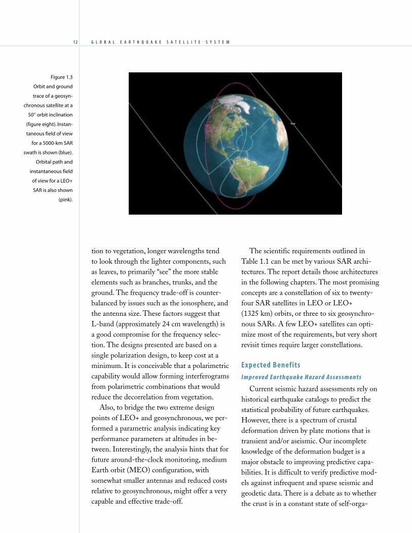
By increasing the satellite elevation even

higher for the purpose of improving its acces-

sibility, one can imagine operating a SAR in a

geosynchronous orbit (Figure 1.3). Such a sys-

tem provides an enormous instantaneous field

of view, and is also able to provide data at very

high resolution, in contrast to optical sensors

at those altitudes. However, the technological

challenges are significant not only because of

the very large active antenna aperture required,

but also due to issues relating to processing

the extremely long apertures, in particular in

Table 1.1

Requirements for

surface deformation

measurements.

MINIMUM GOAL

Displacement Accuracy 25 mm instantaneous 5 mm instantaneous

3–D Displacement Accuracy 50 mm (1 week) 10 mm (1 day)

Displacement Rate 2 mm/yr (over 10 yr) <1 mm/yr (over 10 yr)

Temporal Accessibility (Science) 8 days 1 day or less

Temporal Accessibility (Disaster) 1 day 2 hrs

Daily Coverage 6 × 106 km2 Global (land)

Map Region ±60° latitude Global

Spatial Resolution 50–100 m 3–30 m

Geolocation Accuracy 25 m 3 m

Swath 100 km 500 km

Data Latency in Case of Event 1 day Minutes to hours

1 1

higher resolution modes (2–10 m horizontal).

As a SAR uses the relative motion between

itself and the target to achieve high resolu-

tion, synthetic aperture formation will be im-

possible from a geostationary geometry, where

the radar location is fixed in Earth body fixed

coordinates (EBFC). However, when the in-

clination of the orbit is not zero, the satellite

will be moving in EBFC. We have primarily

studied circular orbits with inclinations be-

tween 50° and 65°. In these cases, the ground

track will resemble that shown in Figure 1.3

(a figure eight). In terms of the Earth surface

area that is in view from a single satellite at

a given time, a geosynchronous satellite will

outperform a LEO-type satellite by two or-

ders of magnitude, thus requiring far fewer

satellites to cover the globe entirely at all

times. The trade-study comparing LEO-type

systems to geosynchronous SAR systems is,

however, complicated for several reasons.

A geosynchronous SAR would require an ex-

tremely large antenna aperture, which would

involve the use of technologies that are not

yet mature. A geosynchronous SAR would

also differ from a LEO SAR in its coverage

characteristics. Contrary to LEO satellites,

a geosynchronous satellite can be placed to

provide focused regional coverage for a lim-

ited set of Earth longitudes. A minimum

of three geosynchronous satellites will be

required for global coverage.

The radar processing required for a geo-

synchronous SAR would also differ quite dra-

matically from that of a LEO system because

of the peculiar characteristics of geosynchro-

nous orbits, as well as atmospheric changes

over the long integration times that arise from

the long apertures and low relative velocities.

It will also be necessary to address dynamic

atmospheric (troposphere and ionosphere)

correction, which is presently not well under-

stood and not tested at all.

In addition, we study constellations based

on those two point designs. The constellations

provide insight as to what future systems

could provide in terms of an operational

mapping capability. Constellations of satellites

capable of providing observations on a very

frequent basis (many observations each day)

were studied for the LEO+, MEO (medium

Earth orbit), and geosynchronous cases. In

these evaluations, the relevant performance

measure was the likelihood that a given posi-

tion on the ground would be mapped within a

given time. The constellations were also as-

sessed for accuracy in providing 3-D displace-

ment measurements.

A key concern in repeat-pass interferom-

etry is so-called temporal decorrelation.

While InSAR measurements reflect the col-

lective displacement of all scatterers within a

given image resolution cell — typically tens of

meters wide to fractional-wavelength accuracy

— the technique breaks down when the scat-

tering centers within the resolution cell expe-

rience different displacements, or when the

dominant scatterers change from one observa-

tion to the next. For example, the vegetation

in the resolution cell might induce temporal

decorrelation. At longer wavelengths, the

radar returns would come mainly from plant

branches and trunks, so the signal might

decorrelate over periods of weeks to months.

At short wavelengths, the radar echoes might

come primarily from the leaves, which can

decorrelate in seconds as the leaves move with

the wind. Precipitation and the freezing or

thawing of the ground will also introduce

significant temporal decorrelation. Longer

wavelengths tend to exhibit better correlation

properties over extended time periods. In rela-

HAZARDSE A R T H Q U A K E . H A Z A R D . A S S E S S M E N T

G L O B A L . E A R T H Q U A K E . S A T E L L I T E . S Y S T E M1 2

tion to vegetation, longer wavelengths tend

to look through the lighter components, such

as leaves, to primarily “see” the more stable

elements such as branches, trunks, and the

ground. The frequency trade-off is counter-

balanced by issues such as the ionosphere, and

the antenna size. These factors suggest that

L-band (approximately 24 cm wavelength) is

a good compromise for the frequency selec-

tion. The designs presented are based on a

single polarization design, to keep cost at a

minimum. It is conceivable that a polarimetric

capability would allow forming interferograms

from polarimetric combinations that would

reduce the decorrelation from vegetation.

Also, to bridge the two extreme design

points of LEO+ and geosynchronous, we per-

formed a parametric analysis indicating key

performance parameters at altitudes in be-

tween. Interestingly, the analysis hints that for

future around-the-clock monitoring, medium

Earth orbit (MEO) configuration, with

somewhat smaller antennas and reduced costs

relative to geosynchronous, might offer a very

capable and effective trade-off.

Figure 1.3

Orbit and ground

trace of a geosyn-

chronous satellite at a

50° orbit inclination

(figure eight). Instan-

taneous field of view

for a 5000-km SAR

swath is shown (blue).

Orbital path and

instantaneous field

of view for a LEO+

SAR is also shown

(pink).

The scientific requirements outlined in

Table 1.1 can be met by various SAR archi-

tectures. The report details those architectures

in the following chapters. The most promising

concepts are a constellation of six to twenty-

four SAR satellites in LEO or LEO+

(1325 km) orbits, or three to six geosynchro-

nous SARs. A few LEO+ satellites can opti-

mize most of the requirements, but very short

revisit times require larger constellations.

Expected Benefits

I m p r o ve d E a r t h q u a k e H a z a r d A s s e s s m e n t s

Current seismic hazard assessments rely on

historical earthquake catalogs to predict the

statistical probability of future earthquakes.

However, there is a spectrum of crustal

deformation driven by plate motions that is

transient and/or aseismic. Our incomplete

knowledge of the deformation budget is a

major obstacle to improving predictive capa-

bilities. It is difficult to verify predictive mod-

els against infrequent and sparse seismic and

geodetic data. There is a debate as to whether

the crust is in a constant state of self-orga-

1 3HAZARDSnized criticality in seismic zones, or whether

the crust approaches and retreats from that

state in a cyclic pattern; the answer has pro-

found implications for the predictability of

earthquakes. One promising model posits that

normalized surface shear strain across faults,

obtainable from dense InSAR data, appears to

be a proxy for the unobservable stress-strain

dynamics that govern fault rupture (Rundle

et al., 2002). The ability to resolve surface

deformation to the centimeter level over the

entire globe will result in hundreds of earth-

quakes each year that can be analyzed to test

and improve predictive models (Melbourne

et al., 2002). Community models will produce

dynamic earthquake hazard assessments by

using observations in real time, mining the

data, and adjusting the earthquake hazard

assessments based on the emerging model

system behavior. This will allow more effec-

tive use of portable ground networks or

arrays of instruments (laser strainmeters,

seismometers, magnetometers) to capture in-

formation on transient fault behavior leading

up to an event. While predicting the time, lo-

cation, and size of a particular earthquake will

remain elusive, much higher fidelity earth-

quake forecasts appear within reach.

The total seismic risk includes the likeli-

hood of a particular seismic event, and the

response of any particular site to the seismic

waves generated. The worst damage occurs

in regions of directed seismic energy, and liq-

uefaction (the sudden liquification of perme-

able sedimentary layers) often amplifies the

damage. Very precise surface deformation

measurements will help to identify aquifer

discharge and recharge, and can provide in-

formation on the saturation of vulnerable

subsurface sedimentary layers (Tobita et al.,

2002). This knowledge can be folded into the

earthquake hazard assessments to produce a

localized, dynamic measure of seismic risk.

Disaster Management

The dynamic earthquake hazard assess-

ments described will provide the disaster

management community with information to

focus mitigation efforts. Such efforts include

prioritizing retrofitting projects to protect

lifelines and infrastructure, educating the

public, staging emergency supplies, and estab-

lishing mobile communication networks.

Earthquake hazard assessment models should

be interfaced with decision support systems

to guide mitigation efforts.

Temporal revisit times on the order of

hours following an event are required to

effectively support disaster response efforts.

Mapping zones of decorrelation will be most

useful to the emergency workers on the

ground. Areas that decorrelate between

interferograms obtained prior to a seismic

event and those that span the event indicate

changes in the built environment, and zones

of intense shaking that can focus response

efforts. InSAR has the advantage of being an

all-weather capability for either day or night,

an important consideration for obtaining

time-critical measurements. Radar-equipped

uninhabited aerial vehicles may play an

important role in disaster response efforts.

A SAR constellation would allow a staring

capability that would reveal the details of

transient postseismic behavior and could be

particularly useful in the hours and days

following a great earthquake to assess the

stress transfer and loading of neighboring

fault systems, potentially predicting large

damaging aftershocks and triggered

earthquakes.

E A R T H Q U A K E . H A Z A R D . A S S E S S M E N T

G L O B A L . E A R T H Q U A K E . S A T E L L I T E . S Y S T E M1 4

Scientific Motivation

he requirements for a global earthquake observational system are

derived from current scientific understanding of earthquake physics,

crustal rheology, and fault interactions, the societal benefits of defining

and mitigating seismic hazard, and aiding in disaster response following

large earthquakes. In simple terms, earthquakes are generally viewed as

being one component of a longer cycle in which a given section of a fault

accumulates stress due to plate tectonic driving forces, releases that stress

during an earthquake, and then begins the cycle anew. Since these time

scales are on the order of seconds for the coseismic portion and centuries

for the interseismic phase, we rarely observe a complete cycle. When

multiple events do repeat on a given fault segment, significant variation

in time scale and earthquake size is the rule. Further complicating our

understanding of earthquakes is that they do not occur in isolation.

Earthquakes located nearby in space and time induce additional forces

into a given fault system, either through the static stress changes induced

coseismically, or through temporally evolving postseismic stress changes.

Since seismology is essentially confined to the coseismic realm, geodesy

is the principal means of measuring the response of the fault and litho-

sphere during the inter- and postseismic part of the earthquake process.

GPS networks have already had a tremendous impact on understanding

the earthquake cycle. A space-based system for monitoring crustal

deformation is the logical next step to achieve revolutionary advances in

earthquake science needed to develop a better predictive capability.

T

Inset: Modeled seismic cycle deformation. (Rundle and Kellogg, 2002)

Background: Interferogram from Antofagasta, Chile, earthquake. (Pritchard et al., 2002)

C H A P T E R

T W O

G L O B A L . E A R T H Q U A K E . S A T E L L I T E . S Y S T E M

1 5

GESS Science Investigations andRequirements

The GESS science requirements derive

directly from the GESS investigations that

addressed the current and future state of our

understanding of earthquake physics, and the

measurements necessary (and practical) to

advance our understanding (see page 98).

Some of the investigations present theoretical

or scenario-based models that predict specific

space–time behavior of seismicity and pat-

terns of crustal deformation. These studies

placed requirements on resolving different

classes of lithospheric models and time scales

of pre- and postseismic deformation. Other

studies presented examples from the current

principal satellite SAR system, the European

Space Agency’s (ESA) ERS satellites, which

have formed the basis for much of our current

understanding of SAR interferometry, both in

terms of performance and in terms of the

types of information and applications that

are possible. These examples impact both the

single image and interferogram data require-

ments, and also illustrate methods for over-

coming some of the error sources through

data stacking, time series inversion, or atmo-

spheric modeling. Finally, applications goals

such as earthquake disaster response also

impact the system requirements.

Before examining the main scientific ques-

tions regarding earthquakes, it is worth sum-

marizing how these pieces fit together and

their historical context. Our current under-

standing and the direction we see as necessary

to understanding the earthquake process are

directly linked to the recent past. Much of

our understanding of earthquakes comes from

seismology, both in terms of their space–time

magnitude, and from understanding the char-

acteristics of the earthquake rupture kinemat-

ics and dynamics. Understanding coseismic

rupture kinematics has benefited from the use

of high-quality geodetic data, in particular the

applications of InSAR.

Advances in GPS and InSAR data in con-

junction with several significant earthquake

sequences (Landers–Hector Mine, California;

Izmit–Duzce, Turkey) in the 1990s provided

important insight into their coseismic rup-

tures, and also provided important new obser-

vations and model constraints on complex

ruptures, triggered earthquake sequences, and

aftershocks. The Landers earthquake was the

first application of InSAR to crustal deforma-

tion. Examination of the complex rupture and

aftershocks of the Landers event stimulated

development of models based on stress shad-

owing and stress migration in the crust and

upper mantle to explain the space-time occur-

rence of these triggered events. The case

was similar for the Izmit–Duzce and Manyi–

Kokoxili, Tibet, earthquake sequences. High-

quality space geodetic data (particularly from

InSAR) allowed observation of spatial and

temporal behavior of the crust following large

earthquakes that forced re-examination of

the crustal response and the forces governing

earthquakes.

The insights gained from these event data

sets have in turn boosted a debate regarding

the time-varying state of stress in the crust,

and have fueled fresh examination of the

physics of the earthquake cycle on fault sys-

tems. Theoretical models that examine earth-

quake clustering and stress evolution predict

spatial and temporal deformation signals that

could be measurable with future satellite sys-

tems. This could lead to significant advances

in our ability to constrain the locations of

future earthquakes.

SCIENCES C I E N T I F I C . M O T I V A T I O N

G L O B A L . E A R T H Q U A K E . S A T E L L I T E . S Y S T E M1 6

Significant improvement in observation

of earthquake crustal deformation provided

by GPS and InSAR during the past decade

placed critical constraints on some existing

models and forced significant revision of

others. Perhaps the most significant inference

we can draw from these advances is that the

feedback loop between data and models is

critical, and that future advances will require

better data, particularly InSAR data.

As stated in Chapter 1, we solicited studies

to define requirements for an observational

system that could address specific outstanding

questions in earthquake science. The results

of the studies are discussed here. In the fol-

lowing section, we have renumbered the

original six study questions slightly, combin-

ing questions 3 and 4 to emphasize the rela-

tionship between complex and triggered

earthquakes, and postseismic processes.

1. How does the crust deform during the interseismic

period between earthquakes and what are its

temporal characteristics (if any) before major

ear thquakes?

Detecting signals precursory to large earth-

quakes has been one of the most sought after

and debated aspects of earthquake physics.

Observations of precursory signals have been

sporadic and often without a clear link to the

subsequent earthquake. In the cases where the

connection is clear, the measurements have

generally been point location measurements,

sometimes requiring measurement sensitivities

that are not possible with satellite systems.

At the core of this debate is whether or

not earthquakes are fundamentally predict-

able. Some have argued that the crust is con-

tinuously in a state of self-organized criticality

(SOC) with the probability of earthquake size

and location remaining steady. Sammis and

Figure 2.1

Evolution of Coulomb

stresses prior to an

earthquake. Each figure

shows the progression

of the surface Coulomb

stress due to earth-

quakes and deep fault

creep on a fault segment

that will experience a

future earthquake. Warm

colors indicate that the

change in stress favors a

future earthquake. Thus,

in addition to the

steady-state tectonic

loading of the future

earthquake segment, the

positive Coulomb stress

caused by the surround-

ing fault segments in-

creases the likelihood of

an event on the future

earthquake segment.

(Sammis and Ivins, 2002)

Seismic SlipFuture Earthquake

Future Earthquake

Future Earthquake

Seismic Slip

Fault Creep

1 7

Ivins (2002) and Rundle and Kellogg (2002)

argue, instead, that earthquake systems have

“memory,” with large earthquakes moving the

crust away from SOC through “stress shadow-

ing” (Fig-ure 2.1). This provides testable ob-

servations of seismicity and late seismic cycle

deformation that could be measured both

seismically and with radar interferometry

(Figure 2.2). The stress shadow models for

the earthquake cycle (Figure 2.1) predict that

when the surrounding crust is moved away

from SOC less background seismicity is ex-

pected, but as a future earthquake approaches

an increase in surrounding activity should

occur.

The basis for this model is the seismicity

and stress shadow models derived for the large

earthquake sequences of the 1990s described

previously. The exciting aspect of these recent

seismic cycle models is that they predict tem-

porally and spatially varying deformation

patterns in the termination regions of locked

fault segments. These models can constrain

earthquake fault system behavior, and should

be of a magnitude measurable with radar sat-

ellite systems.

Part of the model for individual faults and

fault systems consists of sections that experi-

ence either continuous or transient creep.

Creep, or aseismic slip, describes slip on fault

surfaces that does not produce seismic waves,

or discernible shaking. While some creeping

fault segments are recognized, and several

such segments are monitored locally in well-

instrumented regions such as California, many

creeping faults are still unknown. InSAR is a

valuable measurement technique for detecting

and measuring the spatial and temporal char-

acteristics of creeping faults (Figures 2.3 and

2.4), including strike-slip faults (Sandwell and

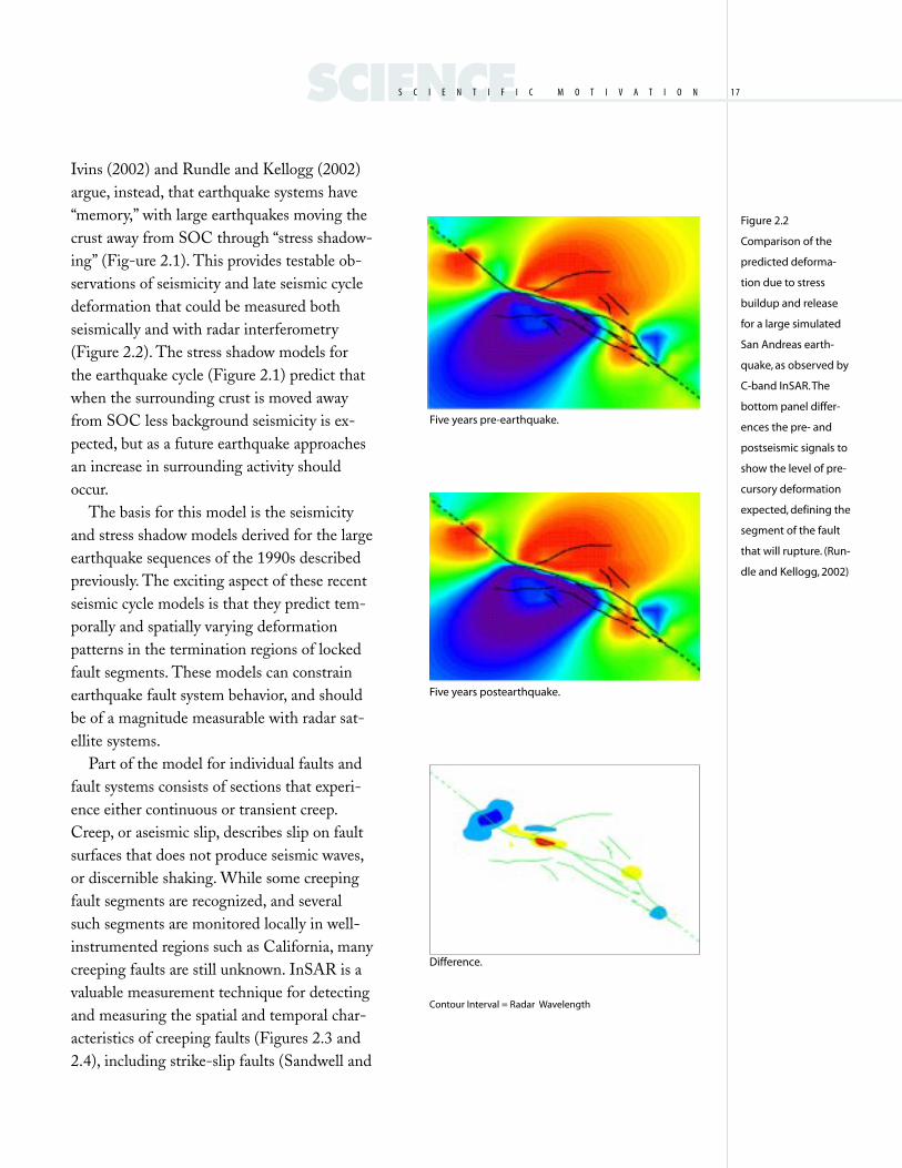
Figure 2.2

Comparison of the

predicted deforma-

tion due to stress

buildup and release

for a large simulated

San Andreas earth-

quake, as observed by

C-band InSAR. The

bottom panel differ-

ences the pre- and

postseismic signals to

show the level of pre-

cursory deformation

expected, defining the

segment of the fault

that will rupture. (Run-

dle and Kellogg, 2002)

SCIENCES C I E N T I F I C . M O T I V A T I O N

Five years pre-earthquake.

Five years postearthquake.

Difference.

Contour Interval = Radar Wavelength

G L O B A L . E A R T H Q U A K E . S A T E L L I T E . S Y S T E M1 8

Fialko, 2002; Burgmann et al., 2002;

Lundgren, 2002) as well as blind thrusts

(Lundgren, 2002). If the motion is steady,

stacking (averaging) InSAR data can reduce

many of the transient and systematic errors

in a series of interferograms (Sandwell and

Fialko, 2002). To detect variations in the rate

of deformation, least-squares network inver-

sions can be used to calculate an InSAR

time series (Figure 2.4), with a relative defor-

mation map at each InSAR data acquisition

(Burgmann et al., 2002; Lundgren, 2002). To

be able to detect any precursory deformation

and to discriminate between even relatively

simple models of locked versus creeping areas

on faults requires a measurement accuracy of

less than 1 mm per year (Zebker and Segall,

2002; Fielding and Wright, 2002).

Figure 2.3

A portion of an inter-

ferogram at Mt. Etna,

Italy, showing anticline

growth and fault creep

(data from 1993–1996,

from ERS-1 and ERS-2,

courtesy ESA). One

color cycle represents

2.8 cm of surface

displacement in the

radar line-of-sight (LOS).

Incidence angle for this

image is approximately

23° from vertical toward

the west-southwest. The

anticline and fault both

show approximately

3 cm of LOS displace-

ment. (Lundgren, 2002)

Requirements

The requirements for detecting these sig-

nals requires both wide swath (on the order

of 100 km), and detailed spatial sampling

(10–100 m). Also required is long-term

temporal continuity (over decades) but at fine

enough temporal sampling (several days) that

precursory phenomena can be separated from

the coseismic, postseismic, and aftershock

signals that accompany a large earthquake

(i.e., Figure 2.2). Similarly, to monitor creep

processes on faults, long time span interfero-

grams (more than seven years) are most im-

portant for resolving rates at the 1 mm/yr level

(Sandwell and Fialko, 2002). However, detect-

ing transient deformation requires weekly or

more frequent measurements to improve tem-

poral resolution and reduce atmospheric noise.

Anticline Growth Fault Creep

1 9

2. How do earthquake ruptures evolve both kinemati-

cally and dynamically and what controls the

earthquake size?

To start to address the question of when

and where a future earthquake will occur,

and how big it will be, requires an improved

understanding of earthquake physics. This

starts with more precise knowledge of the

coseismic ruptures: how does the slip grow

over the fault plane in both time and magni-

tude, and what controls these parameters?

Questions encompassed by this include un-

derstanding how earthquakes nucleate and

what causes them to stop.

Although answering this question has tra-

ditionally been the realm of continuum me-

chanics and seismology, surface deformation

has increasingly played a part in improving

kinematic and dynamic coseismic models.

InSAR has provided detailed surface defor-

mation maps that place tight constraints on

the spatial distribution of slip on the fault

plane, thus allowing seismic data to better

define the temporal evolution of the slip when

joint seismic and geodetic inversions are cal-

culated (Olsen and Peyrat, 2002; DeLouis et

al., 2002).

The location and slip vectors of the

coseismic slip for large earthquakes are impor-

tant in constraining the temporal characteris-

tics of the earthquake rupture, thus defining

the driving force for subsequent postseismic

crustal response, afterslip, and the locations

and sizes of aftershocks. High-density surface

displacements as revealed through InSAR

have been used over the past decade to place

powerful constraints on coseismic slip maps.

When combined with other seismic data, the

resulting inverse models can image the propa-

gation of the rupture in space and time, and

place important constraints on the fault dy-

namics. Repeat orbit interferometry alone

cannot meet the temporal requirements for

directly imaging the seismic wave propagation

and rupture dynamics near the fault. How-

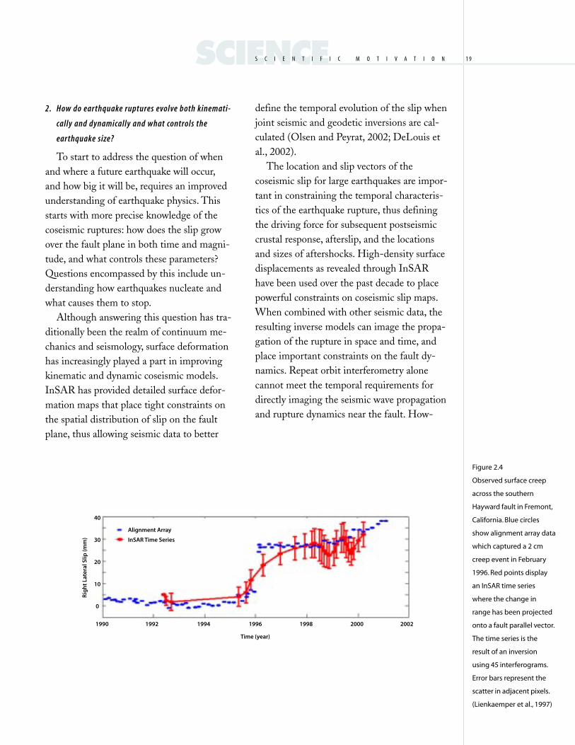
Figure 2.4

Observed surface creep

across the southern

Hayward fault in Fremont,

California. Blue circles

show alignment array data

which captured a 2 cm

creep event in February

1996. Red points display

an InSAR time series

where the change in

range has been projected

onto a fault parallel vector.

The time series is the

result of an inversion

using 45 interferograms.

Error bars represent the

scatter in adjacent pixels.

(Lienkaemper et al., 1997)

SCIENCES C I E N T I F I C . M O T I V A T I O N

Alignment Array

InSAR Time Series

1990 1992 1994 1996 1998 2000 2002

40

30

20

10

0

Rig

ht

Late

ral S

lip (m

m)

Time (year)

G L O B A L . E A R T H Q U A K E . S A T E L L I T E . S Y S T E M2 0

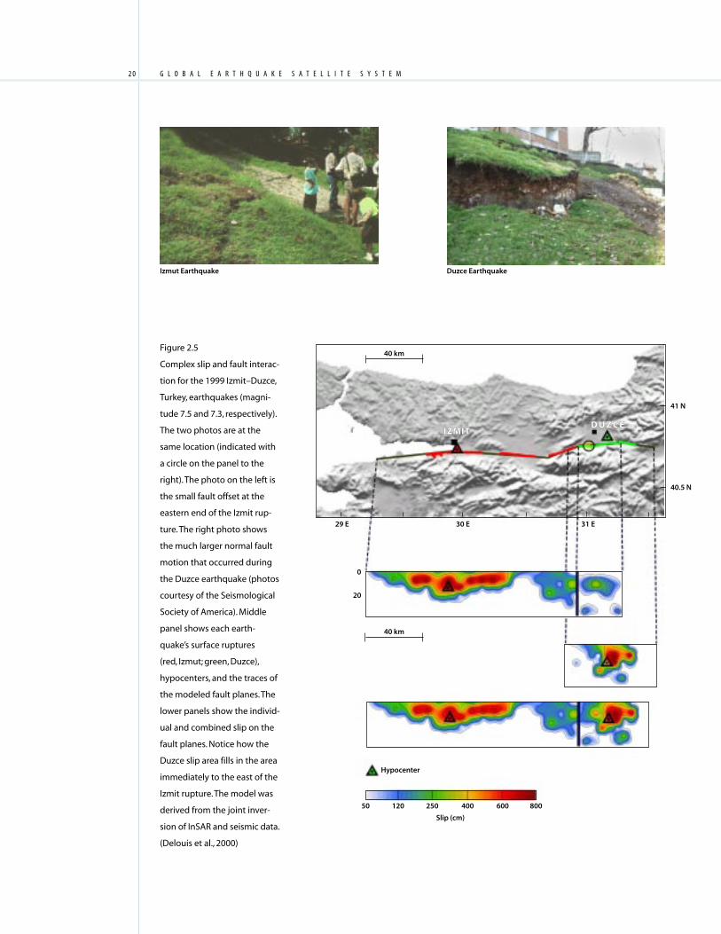
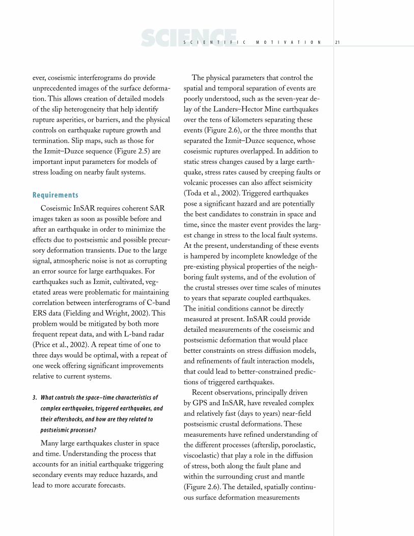
Figure 2.5

Complex slip and fault interac-

tion for the 1999 Izmit–Duzce,

Turkey, earthquakes (magni-

tude 7.5 and 7.3, respectively).

The two photos are at the

same location (indicated with

a circle on the panel to the

right). The photo on the left is

the small fault offset at the

eastern end of the Izmit rup-

ture. The right photo shows

the much larger normal fault

motion that occurred during

the Duzce earthquake (photos

courtesy of the Seismological

Society of America). Middle

panel shows each earth-

quake’s surface ruptures

(red, Izmut; green, Duzce),

hypocenters, and the traces of

the modeled fault planes. The

lower panels show the individ-

ual and combined slip on the

fault planes. Notice how the

Duzce slip area fills in the area

immediately to the east of the

Izmit rupture. The model was

derived from the joint inver-

sion of InSAR and seismic data.

(Delouis et al., 2000)

IZMITIZMITD U Z C ED U Z C E

50 120 250 400 600 800

Slip (cm)

29 E 30 E 31 E

41 N

40.5 N

Hypocenter

40 km

40 km

Izmut Earthquake Duzce Earthquake

0

20

2 1

ever, coseismic interferograms do provide

unprecedented images of the surface deforma-

tion. This allows creation of detailed models

of the slip heterogeneity that help identify

rupture asperities, or barriers, and the physical

controls on earthquake rupture growth and

termination. Slip maps, such as those for

the Izmit–Duzce sequence (Figure 2.5) are

important input parameters for models of

stress loading on nearby fault systems.

Requirements

Coseismic InSAR requires coherent SAR

images taken as soon as possible before and

after an earthquake in order to minimize the

effects due to postseismic and possible precur-

sory deformation transients. Due to the large

signal, atmospheric noise is not as corrupting

an error source for large earthquakes. For

earthquakes such as Izmit, cultivated, veg-

etated areas were problematic for maintaining

correlation between interferograms of C-band

ERS data (Fielding and Wright, 2002). This

problem would be mitigated by both more

frequent repeat data, and with L-band radar

(Price et al., 2002). A repeat time of one to

three days would be optimal, with a repeat of

one week offering significant improvements

relative to current systems.

3. What controls the space–time characteristics of

complex ear thquakes, triggered ear thquakes, and

their aftershocks, and how are they related to

postseismic processes?

Many large earthquakes cluster in space

and time. Understanding the process that

accounts for an initial earthquake triggering

secondary events may reduce hazards, and

lead to more accurate forecasts.

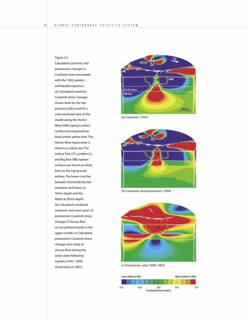
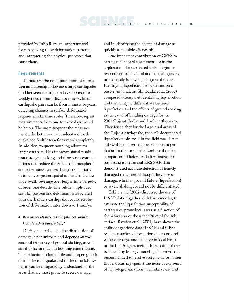
The physical parameters that control the

spatial and temporal separation of events are

poorly understood, such as the seven-year de-

lay of the Landers–Hector Mine earthquakes

over the tens of kilometers separating these

events (Figure 2.6), or the three months that

separated the Izmit–Duzce sequence, whose

coseismic ruptures overlapped. In addition to

static stress changes caused by a large earth-

quake, stress rates caused by creeping faults or

volcanic processes can also affect seismicity

(Toda et al., 2002). Triggered earthquakes

pose a significant hazard and are potentially

the best candidates to constrain in space and

time, since the master event provides the larg-

est change in stress to the local fault systems.

At the present, understanding of these events

is hampered by incomplete knowledge of the

pre-existing physical properties of the neigh-

boring fault systems, and of the evolution of

the crustal stresses over time scales of minutes

to years that separate coupled earthquakes.

The initial conditions cannot be directly

measured at present. InSAR could provide

detailed measurements of the coseismic and

postseismic deformation that would place

better constraints on stress diffusion models,

and refinements of fault interaction models,

that could lead to better-constrained predic-

tions of triggered earthquakes.

Recent observations, principally driven

by GPS and InSAR, have revealed complex

and relatively fast (days to years) near-field

postseismic crustal deformations. These

measurements have refined understanding of

the different processes (afterslip, poroelastic,

viscoelastic) that play a role in the diffusion

of stress, both along the fault plane and

within the surrounding crust and mantle

(Figure 2.6). The detailed, spatially continu-

ous surface deformation measurements

SCIENCES C I E N T I F I C . M O T I V A T I O N

G L O B A L . E A R T H Q U A K E . S A T E L L I T E . S Y S T E M2 2

JJTT

B BB B

L

HM

b/d trans

Moho

(a) Coseismic (1992)

Figure 2.6

Calculated coseismic and

postseismic changes in

Coulomb stress associated

with the 1992 Landers

earthquake sequence.

(a) Calculated coseismic

Coulomb stress changes

shown both for the top

ground surface and for a

cross-sectional view of the

model along the Hector

Mine (HM) rupture surface

(surface encompassed by

black within yellow line). The

Hector Mine hypocenter is

shown as a black star. The

Joshua Tree (JT), Landers (L),

and Big Bear (BB) rupture

surfaces are shown as white

lines on the top ground

surface. The lower crust lies

between the brittle/ductile

transition (b/d trans) at

18 km depth and the

Moho at 28 km depth.

(b) Calculated combined

coseismic and seven years of

postseismic Coulomb stress

changes if viscous flow

occurs predominantly in the

upper mantle. (c) Calculated

postseismic Coulomb stress

changes due solely to

viscous flow during the

seven years following

Landers (1992–1999).

(Freed and Lin, 2001)

20 km

(c) Postseismic only (1999–1992)

Less Likely to Fail More Likely to Fail

–1.0 –0.5 0.0 0.5 1.0Coulomb Stress (bars)

(b) Coseismic and postseismic (1999)

2 3

provided by InSAR are an important tool

for recognizing these deformation patterns

and interpreting the physical processes that

cause them.

Requirements

To measure the rapid postseismic deforma-

tion and afterslip following a large earthquake

(and between the triggered events) requires

weekly revisit times. Because time scales of

earthquake pairs can be from minutes to years,

detecting changes in surface deformation

requires similar time scales. Therefore, repeat

measurements from one to three days would

be better. The more frequent the measure-

ments, the better we can understand earth-

quake and fault interactions more completely.

In addition, frequent sampling allows for

larger data sets. This improves signal resolu-

tion through stacking and time series compu-

tations that reduce the effects of atmospheric

and other noise sources. Larger separations

in time over greater spatial scales also dictate

wide swath coverage over longer time periods,

of order one decade. The subtle amplitudes

seen for postseismic deformation associated

with the Landers earthquake require resolu-

tion of deformation rates down to 1 mm/yr.

4. How can we identify and mitigate local seismic

hazard (such as liquefaction)?

During an earthquake, the distribution of

damage is not uniform and depends on the

size and frequency of ground shaking, as well

as other factors such as building construction.

The reduction in loss of life and property, both

during the earthquake and in the time follow-

ing it, can be mitigated by understanding the

areas that are most prone to severe damage,

and in identifying the degree of damage as

quickly as possible afterwards.

One important contribution of GESS to

earthquake hazard assessment lies in the

application of space-based technologies to

response efforts by local and federal agencies

immediately following a large earthquake.

Identifying liquefaction is by definition a

post-event analysis. Shinozuka et al. (2002)

compared attempts at identifying liquefaction

and the ability to differentiate between

liquefaction and the effects of ground shaking

as the cause of building damage for the

2001 Gujarat, India, and Izmit earthquakes.

They found that for the large rural areas of

the Gujarat earthquake, the well-documented

liquefaction observed in the field was detect-

able with panchromatic instruments in par-

ticular. In the case of the Izmit earthquake,

comparison of before and after images for

both panchromatic and ERS SAR data

demonstrated accurate detection of heavily

damaged structures, although the cause of

damage, whether ground failure (liquefaction)

or severe shaking, could not be differentiated.

Tobita et al. (2002) discussed the use of

InSAR data, together with basin models, to

estimate the liquefaction susceptibility of

earthquake-prone local areas as a function of

the saturation of the upper 20 m of the sub-

surface. Bawden et al. (2001) have shown the

ability of geodetic data (InSAR and GPS)

to detect surface deformation due to ground-

water discharge and recharge in local basins

in the Los Angeles region. Integration of tec-

tonic and hydrologic modeling is needed and

recommended to resolve tectonic deformation

that is occurring against the noise background

of hydrologic variations at similar scales and

SCIENCES C I E N T I F I C . M O T I V A T I O N

G L O B A L . E A R T H Q U A K E . S A T E L L I T E . S Y S T E M2 4

amplitudes. Further, such an integrated model

will contribute to identifying and scaling

liquefaction hazards to determine the total

seismic hazard. These studies will also provide

useful information on the natural periods of

soil sites for earthquake site response analysis.

Requirements

For detection of major liquefaction events,

and major building damage during disaster

response efforts, resolution of 10 m optical

and 15 m SAR is acceptable. A smaller pixel

size would enable a more complete assessment

of ground failure and structural damage. For

rapid earthquake response, revisit times of less

than one day are best, both in terms of the

response time and the quality of the damage

maps. For liquefaction susceptibility and

earthquake site response studies, subcenti-

meter resolution of surface change at spatial

scales of tens of kilometers with revisit times

on the order of a few days would be needed.

5. Are there non-seismic precursory phenomena that

may enable and improve ear thquake prediction?

There are numerous geophysical phenom-

ena other than surface deformation that have

been associated with seismic events.These

include: very low-frequency (VLF), ultra

low-frequency (ULF), and extremely low-fre-

quency (ELF) magnetic fields observed on the

ground and in space, high-frequency electric

fields (including earthquake lights), and ther-

mal anomalies observed with satellite sensors.

There are individual events, such as the 1989

Loma Prieta earthquake ELF magnetic field,

or the warming observed coincident with the

Hector Mine earthquake, that appear signifi-

cantly correlated with seismicity. But contro-

versy remains regarding the statistical

significance of the relationship of these

anomalous signals to seismic events, particu-

larly as earthquake precursors. The very small

number of occurrences of these phenomena

that are properly referenced to background

noise, and which have a clear spatial and tem-

poral relation to specific earthquakes, con-

founds a systematic approach to investigating

the possible sources.

An unusual and unique thermal warming

was observed by Landsat just 18 hours prior

to the Hector Mine earthquake of Octo-

ber 16, 1999 near the Hector Mine fault break

(Crippen, 2002). Comparison of the October

15, 1999 scene to the September 29, 1999

preceding scene shows that greatest warming

in a zone that intersects the Hector Mine

fault break (Figure 1.2). Limited Landsat

coverage of the same region does not reveal a

similar pattern for the Landers earthquake

(1992), but no scene was acquired within

14 days of the Landers quake, and the spatial

and radiometric resolutions and repeat cover-

ages were inferior in the earlier Landsat satel-

lites. The Hector Mine warming has also been

reported in GOES geosynchronous weather

satellite data through a series of images taken

every 30 minutes at 5-km resolution. They

show an unusual (but subtle) heating trend a

few hours before the earthquake.

Earthquake-associated thermal “anomalies”

have previously been reported by others, but

without the spatial or temporal clarity of

“signal” possibly indicated by the Hector

Mine observations. Thermal emissions associ-

ated with earthquakes have been attributed to

changes in fluid flow near fault zones resulting

from rupturing of flow barriers as the crust

approaches its yield strength (e.g., Hamza,

2001). While pressure-driven fluid flow

2 5

within a shallow fault zone could generate a

thermal anomaly of the scale and amplitude

observed, a high permeability of the affected

layers would be required for a precursory

signal within one month of a main shock

(E. Ivins, personal communication, 2003).

This mechanism has been proposed as a

means of generating both thermal and electro-

magnetic anomalies associated with the Loma

Prieta earthquake (Fenoglio et al., 1995). To

date, no clearly quantified relationship has

emerged between thermal emission signals

and earthquakes, either preseismically or

coseismically. If thermal anomalies precede

earthquakes by hours to days, satellite obser-

vations will require both high temporal

(hourly) and high spatial (< 100 m) resolution

to capture the signal.

Precursory quasicontinuous electric and

magnetic fields associated with earthquakes,

when they can be confidently observed, ap-

pear to arise from electrokinetic effects of

fluid flow (Fenoglio et al., 1995; Park, 1996).

Coseismic signals observed near the epicenter

may reflect piezomagnetic effects ( Johnston,

1997). Whereas a strong signal was observed

by Magsat at 4 Hz for a M 7.2 earthquake in

Tonga in 1980, a search for magnetic field

signals of recent earthquakes using three cur-

rently orbiting high-precision magnetic field

satellites did not identify any promising

correlations (Taylor and Purucker, 2002).

The mechanism proposed for Loma Prieta,

invoking the motion of a conductive fluid re-

sulting from rupture of impermeable layers,

has also been proposed to explain transient

thermal anomalies. Progress in understanding

the relationship of electromagnetic and ther-

mal emissions to the earthquake cycle requires

high-quality, frequently updated observations,

and verifiable models that satisfy multiple ob-

servational constraints.

Requirements

High spatial (< 100 m) resolution thermal

measurements between 3 and 15 microns, up-

dated hourly to daily, are needed to capture

putative ephemeral thermal anomalies associ-

ated with earthquakes. Continuous magnetic

and electric field measurements at DC to

800 Hz frequency are needed to test whether

variations are correlated with seismic activity.

Most importantly, these signals must be sys-

tematically isolated from natural background

noise in a consistent manner, and evaluated

simultaneously with crustal stress inferred

from surface deformation measurements and

fluid motion in the crust inferred from time-

varying gravity.

The detailed science requirements dis-

cussed above constitute a complete set of ob-

servations that contribute to understanding

earthquake physics and the earthquake cycle.

However, consistent with the recommenda-

tions of the SESWG report and the wider

community, we have focused our mission ar-

chitecture on observing surface deformation,

as this is deemed the highest payoff measure-

ment to study earthquake physics. We focus

on InSAR rather than LIDAR for three rea-

sons. InSAR is an all-weather capability that

can efficiently map the globe using a wide

swath. It also measures topographic change

to fractional wavelength accuracy. Its major

limitation is in dense vegetation, and loss of

correlation due to major surface disruption or

vegetation change unrelated to tectonics.

LIDAR can provide very precise “bare-earth”

SCIENCES C I E N T I F I C . M O T I V A T I O N

G L O B A L . E A R T H Q U A K E . S A T E L L I T E . S Y S T E M2 6

topography beneath vegetation. Its limitations

are inoperability in cloudy air, a narrow

footprint, and less-precise surface change

detection. The InSAR technique has clear

advantages for measuring long-term surface

deformation globally. However, the LIDAR

technique is likely to be important for local

and regional-scale surveys of paleoseismic

landforms, and for change detection beneath

vegetation canopy.

The derived requirements for monitoring

surface deformation are summarized on the

science roadmap of Figure 2.7.

Disaster Management

A Global Earthquake Satellite System

could contribute to managing earthquake di-

sasters in two ways: by enabling higher spatial

and temporal resolution hazard maps, and by

Figure 2.7

Science measurement

requirements for surface

displacement.

0.1

5

10

20

50

3-D

Dis

pla

cem

ent

Acc

ura

cy (m

m)

102 10 1

Revisit Frequency (days)

0.1 10–2

INTERSEISMIC STRAIN

• Steady state

• Requires long-time

series (10-yrs)

TRANSIENT DEFORMATION

• Stress transfer

• Triggered earthquakes

• Aseismic slip

• Slow earthquakes

• Postseismic relaxation

• Afterslip

• Static rupture

COSEISMIC OFFSETS DYNAMIC RUPTURES

providing timely and valuable information

following an earthquake. Hazard assessments

are currently used proactively to guide both

building codes and disaster preparedness.

Spatio-temporal granularity of hazards

assessments would allow prioritizing of retro-

fitting projects according to relative seismic

risks. Similarly, emergent behavior of a fault

system indicating increasing potential for fault

rupture would allow preparations to focus on

specific geographic areas and infrastructure

assets. In a post-event scenario, GESS would

provide maps showing major damage and

mapping peak accelerations to accurately as-

sess the magnitude of the damage and guide

first-response teams. It would also provide

data for real-time mapping of changes in

stress on neighboring fault systems to assess

potential triggered seismicity.

2 7

The needs of the disaster management

community drive the latency requirements for

downlinking data and producing data prod-

ucts. Data must reach the ground very quickly,

and be processed into interferograms within

hours of an event to maximize its effective-

ness. Direct downlink to users and a distrib-

uted processing environment enable this

scenario. Data and data products must be

released immediately on the Web, and online

catalogs of recent data acquisitions, interfero-

grams, and deformation time series must be

maintained to expedite processing. Near-line

archives of a decimated complete data set are

also required to facilitate new analyses. Maps

would be produced showing areas where the

radar returns have decorrelated to indicate

changes in the built environment, as well as

maps of peak accelerations showing locations

of major damage.

A robust community modeling environ-

ment is necessary to support the disaster

management community. The community

model would provide a sanctioned way to

identify emergent behavior of a fault system

and adjust hazard maps. Processing of data

would be expedited following anomaly detec-

tion (precursors), and ground networks de-

ployed to further investigate and monitor

fault behavior. Following an event, the model

would produce an estimate of the new stress

field.

The customers for this information are

anticipated to be the USGS, the Federal

Emergency Management Agency (FEMA),

California Office of Emergency Services

(CA OES), local governments, and schools.

Enlightening the general public to the

dynamic nature of crustal deformation and

therefore the hazards they must live with

should lead to greater overall preparedness

and thus fewer losses.

SCIENCES C I E N T I F I C . M O T I V A T I O N

G L O B A L . E A R T H Q U A K E . S A T E L L I T E . S Y S T E M2 8

T he GESS enhanced low-Earth orbit concept, or LEO+, proposes the operation

of one or more L-band SAR systems at an altitude of approximately 1325 km,

significantly higher than those of most current SAR platforms. The higher platform

altitude affords a wider visible area to the sensor: two 800-km swaths, each

comprising seven subswaths, from 300 to 1100 km on either side of the satellite

ground track. The large viewable area enables the system to access the entire

Earth quickly, reducing the interferometric repeat period to six days and allowing

for much finer InSAR temporal resolution than is available from other current or

pending SAR missions. The higher altitude also offers better orbit stability, another

important consideration for repeat-pass interferometry. A LEO+ mission could be

flown using existing conventional technology, though the system would require

a slightly larger antenna and greater power than LEO SAR systems.

The radar would be capable of generating high-resolution single-subswath images

in a standard stripmap mode and provide lower-resolution, wider-swath images

from multiple subswaths in interferometric ScanSAR mode. In stripmap mode,

the five-look image resolution would be 30 × 30 m or better. The interferometric

surface-displacement accuracy would depend mainly on the temporal correlation

properties of the surface under observation, as well as on atmospheric effects, but

with appropriate calibration and post-processing, nominal line-of-sight displace-

ment accuracies better than 1 cm can be achieved. The instrument would acquire

right-looking and left-looking data on ascending and descending passes, so it

would be possible to synthesize 3-D maps of surface displacement from multiple

interferograms with different viewing angles. Over targeted areas, a high-resolution

3-D displacement map comprising ten or more individual images could be gener-

ated in under 12 days, and global maps generated annually.

C H A P T E R

T H R E E

Enhanced Low-Earth Orbit

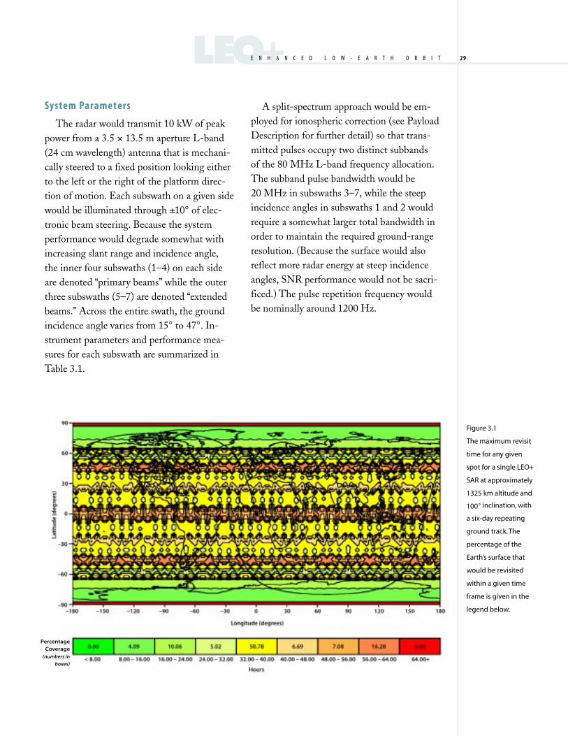
2 9LEO+E N H A N C E D . L O W - E A R T H . O R B I T 2 9

Figure 3.1

The maximum revisit

time for any given

spot for a single LEO+

SAR at approximately

1325 km altitude and

100° inclination, with

a six-day repeating

ground track. The

percentage of the

Earth’s surface that

would be revisited

within a given time

frame is given in the

legend below.

System Parameters

The radar would transmit 10 kW of peak

power from a 3.5 × 13.5 m aperture L-band

(24 cm wavelength) antenna that is mechani-

cally steered to a fixed position looking either

to the left or the right of the platform direc-

tion of motion. Each subswath on a given side

would be illuminated through ±10° of elec-

tronic beam steering. Because the system

performance would degrade somewhat with

increasing slant range and incidence angle,

the inner four subswaths (1–4) on each side

are denoted “primary beams” while the outer

three subswaths (5–7) are denoted “extended

beams.” Across the entire swath, the ground

incidence angle varies from 15° to 47°. In-

strument parameters and performance mea-

sures for each subswath are summarized in

Table 3.1.

A split-spectrum approach would be em-

ployed for ionospheric correction (see Payload

Description for further detail) so that trans-

mitted pulses occupy two distinct subbands

of the 80 MHz L-band frequency allocation.

The subband pulse bandwidth would be

20 MHz in subswaths 3–7, while the steep

incidence angles in subswaths 1 and 2 would

require a somewhat larger total bandwidth in

order to maintain the required ground-range

resolution. (Because the surface would also

reflect more radar energy at steep incidence

angles, SNR performance would not be sacri-

ficed.) The pulse repetition frequency would

be nominally around 1200 Hz.

PercentageCoverage

(numbers in

boxes)

G L O B A L . E A R T H Q U A K E . S A T E L L I T E . S Y S T E M3 0

1 2 3 4 5 6 7

Ground Range from 300/450 445/595 590/740 735/835 830/930 925/1025 1020/1090

Nadir (km, near/far)

Look Angle 12.7/18.5 18.4/23.7 23.5/28.4 28.2/31.1 31.0/33.6 33.5/36.0 35.8/37.4

(deg, near/far)

Incidence Angle 15.4/22.6 22.3/29.1 28.8/35.0 34.8/38.6 38.4/42.0 41.8/45.2 45.0/47.2

(deg, near/far)

Transmit Power 10.0 10.0 10.0 10.0 10.0 10.0 10.0

(peak, kW)

Pulse Duration (µs) 50.0 50.0 50.0 50.0 50.0 50.0 50.0

Bandwidth (MHz) 17.0 12.0 10.0 10.0 10.0 10.0 10.0

Polarization HH HH HH HH HH HH HH

Pulse Repetition 1240 1191 1233 1178 1224 1176 1220

Frequency (Hz)

Ground Range Resolution 28.8/19.9 28.5/22.3 26.9/22.6 22.7/20.8 20.9/19.4 19.5/18.3 18.4/17.7

(m, near/far)

Single-Look Azimuth 6.0 6.3 6.0 6.3 6.1 6.3 6.1

Resolution (m)

Minimum SNR Assuming 10.4 9.8 9.6 11.1 11.0 10.3 10.3

Model Soil Surface (dB)

Maximum Range –35.0 –36.0 –29.5 –32.8 –26.8 –23.7 –20.1

Ambiguity Level (dB)

Maximum Azimuth –22.1 –20.9 –21.8 –20.4 –21.7 –20.5 –21.5

Ambiguity Level (dB)

Data Rate (Mb/s) 142.7 124.6 128.6 95.2 105.9 107.8 84.9

Table 3.1

LEO+ beam

summary.

Orbit, Coverage, and Constellations

The satellite would be launched into a

nearly circular, sun-synchronous terminator

orbit at an altitude of 1325 km and an inclina-

tion of 101°; this orbit has a six-day repeating

ground track (Figure 3.1). The satellite would

be controlled under tight attitude and trajec-

tory constraints in order to facilitate repeat-

pass interferometric processing. Given the

satellite orbit and the capabilities of the radar

instrument, 85% of the Earth’s surface would

be viewable by the satellite within 24 hours,

and 100% of the surface would be viewable

within 60 hours. This quick-response capabil-

ity of the SAR could provide timely data in

the crucial hours and days following an earth-

quake or other natural disaster.

3 1LEO+E N H A N C E D . L O W - E A R T H . O R B I T 3 1

Figure 3.2

A comparison of

cumulative land

coverage by different

LEO and LEO+

constellations. A

four-satellite LEO+

constellation covers

90% of the Earth in

six hours.

Perc

ent

Cu

mu

lati

ve L

and

Co

vera

ge

100

90

80

70

60

50

40

30

20

10

06 12 18 24 30 36 42 48 54 60 66 72

Time (hours)

1 LEO +

2 LEO +

4 LEO +

1 LEO

2 LEO

4 LEO

8 LEO

A constellation of identical satellites in

phased, node-spaced orbits could provide

even shorter interferometric repeat times and

event-response times (see Figure 3.2).

With a constellation of four satellites, the

interferometric repeat period could be reduced

to 36 hours, and an image of any point on the

Earth could be formed by at least one satellite

within about 12 hours of an event (or six hours

for 85% accessibility). Multiple satellites could

also be placed at different orbital inclinations

in order to enhance the achievable 3-D sur-

face displacement accuracy. That is, while

near-polar orbits are required to provide Earth

coverage at high latitudes, they do not offer

much diversity in viewing angle at very low

and very high latitudes. Hence, in equatorial

regions of the Earth for example, the north–

south component of surface displacement

could not be very accurately determined.

Therefore, in addition to the satellite(s) in-

clined 101°, one or more satellites could be

placed in lower-inclination orbits in order to

increase the orthogonality of the directions

from which different areas are mapped

(Figure 3.3).

A more ambitious constellation of 36 satel-

lites could reduce the interferometric repeat

time to four hours and could allow most

points on the Earth to be imaged within

around two hours or less.

Instrument and Operational Modes

Each satellite could be operated in both

high-resolution, single-subswath stripmap

modes and wide-area, multiple-subswath in-

terferometric ScanSAR modes (100-m reso-

lution at eight looks). Note that in the

interferometric ScanSAR modes, the instru-

ment would need to be timed such that

corresponding ScanSAR bursts are aligned

between successive orbit passes. This mode

of operation has not been demonstrated, but

we expect that it is feasible.

If the instrument collects data for one-third

of the time it is over land, its operational duty

cycle would be approximately 10% on average,

G L O B A L . E A R T H Q U A K E . S A T E L L I T E . S Y S T E M3 2

Figure 3.3

Maximum 3-D

accuracy from two

LEO+ satellites at

101° and 30° inclina-

tions, assuming

1 cm line-of-sight

displacement.

though the duty cycle might be significantly

higher for some orbits. Each year, the instru-

ment’s operational plan would most likely

include the collections of different global

data sets in various high- and low-resolution

modes for archive in an interferometric library

(see Table 3.2).

The satellite would also be tasked to

collect data as frequently as possible from im-

portant seismogenic areas, such as Southern

California and other parts of western North

America, in addition to other seismogenic

zones in South America, Asia, the Mediterra-

nean, and others.

A typical six-month operational plan might

consist of 36 days spent acquiring a global,

low-resolution, primary-beam, interferometric

ScanSAR data set, and 144 days spent acquir-

ing four to six high-resolution maps of

western North America and two to three

high-resolution maps of other key areas. As

possible, data would also be acquired over

other areas to fill in coverage for global high-

resolution maps.

The ground resolution depends on which

operational mode is in use. The ground reso-

lution for both primary (1-4) and extended

beams (5-7) is 30 m in stripmap mode, and

100 m in ScanSAR. The number of looks

available also changes for different modes both

across and between subswaths. The primary

beams have five looks in stripmap mode, and

14 in ScanSAR mode; while the extended

beams have five looks in stripmap mode, but

18 looks for ScanSAR. The ground swath for

each beam can be calculated from the ground

range values in Table 3.1. For stripmap mode,

the ground swath in beams 1-7 in kilometers

is: 150, 150, 150, 100, 100, 100, 70. In

ScanSAR mode, however, the primary-beam

ground swath is 535 m, and the extended-

beam ground swath is 260 m. Additional

PercentageCoverage

(numbers in

boxes)

3 3LEO+E N H A N C E D . L O W - E A R T H . O R B I T 3 3

Table 3.2

LEO+ operational

modes.

Global Primary-Beam ScanSAR (6 days) * (2 sides) / (0.333 over-land duty cycle) 36 days

Global Extended-Beam ScanSAR (6 days) * (2 sides) / (0.333 over-land duty cycle) 36 days

Priority-Area Primary-Beam Stripmap (6 days) * (2 sides) * (4 beams) 48 days

Priority-Area Extended-Beam Stripmap (6 days) * (2 sides) * (3 beams) 36 days

Global Fill-In Primary-Beam Stripmap (6 days) * (2 sides) * (4 beams) 96 days

(Targeted Area Time) (0.333 over-land duty cycle)

Global Fill-In Extended-Beam Stripmap (6 days) * (2 sides) * (3 beams) 72 days

(Targeted Area Time) (0.333 over-land duty cycle)

instrument parameters do not vary for sub-

swath or operational mode:

• RF peak power is 10 kW

• Average orbit duty cycle is 10%

• Peak DC power is 3816 W

An illustration of the operational modes

and beams is shown in Figure 3.4.

Per formance

While the studied system parameters do

not represent a final, fully optimized design,

they maintain a signal-to-noise ratio of at

least 10 dB over the entire visible area, assum-

ing a model scattering profile for a soil surface

and incidence angles determined by a nominal

spherical Earth. The preliminary design yields

a range ambiguity level below –30 dB in

the primary subswaths and –20 dB in the ex-

tended subswaths, and an azimuth ambiguity

below –20 dB in any subswath. Note also that

the overall performance is generally better in

the middle of a subswath than at its edges,

and that the subswath widths can be increased

slightly if reduced performance is acceptable

in the extended areas. For the stripmap

modes, the nominal along-track (azimuth)

resolution would be 6 m, and the nominal

cross-track (range) resolution projected

onto the ground would be 30 m or better.

Performance parameters are summarized in

Table 3.1, referenced previously in the

System Parameters section.

The interferometric displacement accuracy

of the system would be highly dependent

upon the properties of the surface and the

atmosphere at the time data is acquired.

Under ideal conditions, line-of-sight displace-

ment accuracies of a few millimeters might

be possible from a single interferogram at

30 m resolution, but the performance would

degrade considerably in the presence of tem-

poral decorrelation or atmospheric variability.

Temporal decorrelation comes about when,

rather than bulk displacement, the surface

exhibits random change that makes the

interferometric phase noisier.

Decorrelation-induced phase noise tends to

become more severe as the temporal baseline

is increased, but it can also be reduced

through averaging, either spatially or over

multiple interferometric pairs. Atmospheric

artifacts result from the spatial and temporal

variations in the effective radar signal path

length related to changes in the propagation

properties of the troposphere and ionosphere.

These artifacts are more difficult to remove,

G L O B A L . E A R T H Q U A K E . S A T E L L I T E . S Y S T E M3 4

Figure 3.4

LEO+ operational

modes.

1325 km Altitude

300 km

150 km

Primary Beams

Extended Beams

Stripmap535 km

100 km Stripmap

260 km

ScanSAR

Nadir Track

Flight Direction

but some mitigation strategies are possible

(see the Atmospheric Mitigation section in

Chapter 5). We expect that average-case accu-

racies of a few centimeters or better would be

possible from a single interferogram, and that

these accuracies might be reduced to the

subcentimeter level with the proper combina-

tion of multiple data sets. (This underscores

the need for an InSAR mission that can ac-

quire large amounts of data over short time

periods for targeted areas.) We also expect

subcentimeter 3-D displacement accuracies

for regions between ±30-70° latitude, though

as described previously, one of the 3-D dis-

placement components may be indetermin-

able for other latitudes if data are acquired

only from satellites at the same near-polar

orbital inclination.

Data Rates and Volumes

The average instantaneous data rate of the

satellite would be approximately 105 Mb/s, so

assuming a 10% instrument duty cycle, the

data volume collected each day would be about

950 Gb, or 119 GB. Over five years, the satel-

lite would collect more than 200 TB of data

that would need to be archived. For downlink

and instrument-storage sizing, the maximum

instantaneous data rate of 320 Mb/s and a

25% instrument duty cycle would yield

250 Gb of data per orbit. See the Ground Data

System section in this chapter for more detail.

Payload Description

The LEO+ mission described here consists

of an L-band SAR instrument on a dedicated

spacecraft. The radar antenna, consisting of

ten lightweight rigid panels and antenna de-

ployment structure, comprises the majority of

the radar instrument’s 640 kg mass (including

30% contingency). The radar sensor electronics

subsystem, which generates the transmit wave-

form and receives the return echoes, include

the RF electronics, data handling electronics,

and timing and control electronics.

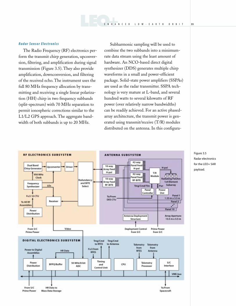
3 5LEO+E N H A N C E D . L O W - E A R T H . O R B I T 3 5

Figure 3.5

Radar electronics

for the LEO+ SAR

payload.

R a d a r S e n s o r E l e c t r o n i c s

The Radio Frequency (RF) electronics per-

form the transmit chirp generation, upconver-

sion, filtering, and amplification during signal

transmission (Figure 3.5). They also provide

amplification, downconversion, and filtering

of the received echo. The instrument uses the

full 80 MHz frequency allocation by trans-

mitting and receiving a single linear polariza-

tion (HH) chirp in two frequency subbands

(split-spectrum) with 70 MHz separation to

permit ionospheric corrections similar to the

L1/L2 GPS approach. The aggregate band-

width of both subbands is up to 20 MHz.

Subharmonic sampling will be used to

combine the two subbands into a minimum-

rate data stream using the least amount of

hardware. An NCO-based direct digital

synthesizer (DDS) generates multiple chirp

waveforms in a small and power-efficient

package. Solid-state power amplifiers (SSPAs)

are used as the radar transmitter. SSPA tech-

nology is very mature at L-band, and several

hundred watts to several kilowatts of RF

power (over relatively narrow bandwidths)

can be readily achieved. For an active phased-

array architecture, the transmit power is gen-

erated using transmit/receive (T/R) modules

distributed on the antenna. In this configura-

G L O B A L . E A R T H Q U A K E . S A T E L L I T E . S Y S T E M3 6

tion, we assume roughly 25 W per module,

where 420 modules are distributed along the

array to achieve the 10 kW minimum trans-

mit power. The front-end electronics control

the signal routing of the primary, redundant,

and test/calibration signals. The receiver

downconverts the echo received from the an-

tenna and frequency translates the two split-

spectrum subbands using a subharmonic

sampling technique to produce two concat-

enated frequency bands at range-offset video.

Gain control provides high dynamic range.

These signals are then routed to the data han-

dling system for digitization and storage.

The data handling hardware consists of

the high-speed analog-to-digital converter

(ADC), data buffer and block floating-point

quantizer (BFPQ). For the subharmonic sam-

pling receiver, the ADC sample clock is only

required to be 50 MHz, with an analog band-

width of 80 MHz, sampling at 8 bits per

sample. The BFPQ converts the 8-bit data to

4-bit data and the buffer reduces the peak

data rate to interface with the solid-state re-

corder (SSR). Formatting includes embedding

a synch word, frame count, and spacecraft

data (GPS, time) into the data stream. Only

one high-rate data channel is required.

The radar control, timing, and telemetry

hardware includes a central processor unit

(CPU), telemetry processor, spacecraft inter-

face module, radar control and timing unit

(CTU), and power module. A dedicated CPU

is implemented to control and manage the

instrument functions and data flow. This

approach ensures a simple interface to the

spacecraft and aides in ground testing of the

instrument. While the CTU generates deter-

ministic subsecond timing parameters, the

CPU controls operations for time scales

greater than one second (ScanSAR control

parameters, radar mode, data flow). The dedi-

cated CPU will be able to easily handle the

control algorithm to calculate and store in a

look-up table the beam position for ScanSAR

operation. Based upon the command word

generated by the CPU, the CTU generates

the timing signals necessary to control the ra-

dar, including pulse repetition frequency

(PRF), receiver protection and gain control,

antenna phase shifter settings, and data win-

dow position.

The radar electronics will be housed in two

separate chassis, one for the RF electronics and

one for the digital electronics. Each subsystem

has its own dedicated power distribution unit

to convert the raw spacecraft voltages to the

required DC voltages and to condition and

distribute them to the subsystems. Full block

redundancy of the radar electronics is imple-

mented to achieve the five-year mission life-

time. The RF electronics consist of primary

and redundant subassemblies and the Redun-

dancy/Built-In-Test select switch matrix, each

packaged in a separate shielded enclosure.

Surface-mount RFIC/MMIC technology in

microstrip circuits ensures cost-effective, low-

mass packaging. The digital electronics will

reside in a standard VME chassis. Standard

VME architecture enables the use of several

existing commercial-off-the-shelf (COTS)

hardware assemblies to reduce cost and risk.

These include the CPU board, the Telemetry

Processor Board, the spacecraft I/O interface

board, and the power distribution and condi-

tioning board. The custom digital hardware

uses FPGA technology to reduce size and

power while increasing flexibility of the design.

R a d a r A n t e n n a

The antenna performs the beam steering

and transmission function as well as high-

power amplification on transmit and low-noise

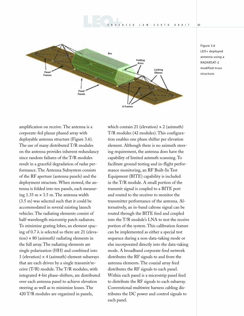
3 7LEO+E N H A N C E D . L O W - E A R T H . O R B I T 3 7

Figure 3.6

LEO+ deployed

antenna using a

RADARSAT-2

modified truss

structure.

Bus

FoldingArms

LockingElbows

FixedPanels

A-Frames

PanelFrames

amplification on receive. The antenna is a

corporate-fed planar phased array with

deployable antenna structure (Figure 3.6).

The use of many distributed T/R modules

on the antenna provides inherent redundancy

since random failures of the T/R modules

result in a graceful degradation of radar per-

formance. The Antenna Subsystem consists

of the RF aperture (antenna panels) and the

deployment structure. When stowed, the an-

tenna is folded into ten panels, each measur-

ing 1.35 m × 3.5 m. The antenna width

(3.5 m) was selected such that it could be

accommodated in several existing launch

vehicles. The radiating elements consist of

half-wavelength microstrip patch radiators.

To minimize grating lobes, an element spac-

ing of 0.7 λ is selected so there are 21 (eleva-

tion) × 80 (azimuth) radiating elements in

the full array. The radiating elements are

single polarization (HH) and combined into

1 (elevation) × 4 (azimuth) element subarrays

that are each driven by a single transmit/re-

ceive (T/R) module. The T/R modules, with

integrated 4-bit phase-shifters, are distributed

over each antenna panel to achieve elevation

steering as well as to minimize losses. The

420 T/R modules are organized in panels,

which contain 21 (elevation) × 2 (azimuth)

T/R modules (42 modules). This configura-

tion enables one phase shifter per elevation

element. Although there is no azimuth steer-

ing requirement, the antenna does have the

capability of limited azimuth scanning. To

facilitate ground testing and in-flight perfor-

mance monitoring, an RF Built-In Test

Equipment (BITE) capability is included

in the T/R module. A small portion of the

transmit signal is coupled to a BITE port

and routed to the receiver to monitor the

transmitter performance of the antenna. Al-

ternatively, an in-band caltone signal can be

routed through the BITE feed and coupled

into the T/R module’s LNA to test the receive

portion of the system. This calibration feature

can be implemented as either a special test

sequence during a non-data-taking mode or

else incorporated directly into the data-taking

mode. A broadband corporate feed network

distributes the RF signals to and from the

antenna elements. The coaxial array feed

distributes the RF signals to each panel.

Within each panel is a microstrip panel feed

to distribute the RF signals to each subarray.

Conventional multiwire harness cabling dis-

tributes the DC power and control signals to

each panel.

G L O B A L . E A R T H Q U A K E . S A T E L L I T E . S Y S T E M3 8

Table 3.3

Instrument mass

and power for GESS

LEO+ mission.

PEAK DC STANDBY ORBIT POWER

QUANTITY MASS (KG) POWER (W) POWER (W) AVG (W)

Antenna Subsystem 433.0 2783.3 13.3 278.3

T/R Modules 420 43.0 2066.7 0.0

Panels (Aperture, Panel RF Feed, Frame, Hinges) 10 298.0 0.0 0.0

Antenna Panel Electronics 10 10.0 160.0 10.7

Antenna DC–DC Converters 67 10.0 556.73 2.7

Antenna Array RF Feed — 10.0 0.0 0.0

Antenna Power and Control Cabling — 15.0 0.0 0.0

Deployment Structure 1 47.0 0.0 0.0

Interface Structure and Launch Support s/c 0.0 0.0 0.0

Actuators and Release Mechanisms s/c 0.0 0.0 0.0

Thermal Blankets (MLI) s/c 0.0 0.0 0.0

Radio Frequency Electronics Subsystem 29.0 91.1 11.1 9.1

Chirp Generator 2 2.0 12.0 0.0

Frequency Synthesizer 2 3.0 20.0 10.0

Upconverter 2 2.0 7.0 0.0

Driver 2 4.0 28.0 0.0

Receiver 2 2.0 3.0 0.0

Red and BITE Select 1 1.0 12.0 0.0

Power Distribution 2 3.0 9.1 1.1

Housing, Cabling, and Misc. 1 12.0 0.0 0.0

Digital Electronics Subsystem 31.0 61.3 41.3 6.1

Timing and Control Unit 2 2.0 7.0 7.0

ADC/Buffer 2 3.0 10.0 0.0

BFPQ 2 2.0 6.0 0.0

CPU 2 2.0 10.0 10.0

Telemetry 2 2.0 10.0 10.0

S/C I/F and Data Formatter 2 2.0 6.0 6.0

Power 2 3.0 12.3 8.3

Housing, Cabling, and Misc. 1 15.0 0.0 0.0

Radar Total 493.0 2935.7 65.7 293.5

30% Margin 147.9 880.7 19.7 88.1

GESS Radar Total w/ Margin 640.9 3816.4 85.4 381.6

3 9LEO+E N H A N C E D . L O W - E A R T H . O R B I T 3 9

The antenna structure is a deployable truss

structure, which provides both support and

strength to the panels and maintains flatness

of the full array. The structure and deployment

mechanisms must be reliable and lightweight

and must deploy such that the antenna is flat,

structurally stiff, and thermally stable. The

flatness requirement of the antenna is one-

sixteenth of a wavelength (1.4 cm) to mini-

mize antenna pattern distortion. Two com-

peting truss structures are suitable for this

application. A modified deep-truss structure

(as used in Seasat and RADARSAT-2) has

extensive heritage and is considered relatively

low risk. The edge-truss structure offers a

very compact stowed envelope although it is

less mature technologically. Both are very

lightweight and can meet all GESS structural

requirements. The spacecraft provides the

interface, launch support structure, and ther-

mal blankets. The instrument mass and

power are shown in Table 3.3.

H e r i t a g e

While the instrument is based on existing

technology, it represents a major leap forward

in measurement capability. The GESS L-band

SAR instrument derives much design and

hardware heritage from its SIR-C predecessor.

SIR-C experimentally validated several new

SAR techniques including ScanSAR, spotlight

SAR, and repeat-pass interferometry. Technol-

ogy development activities following the suc-

cess of SIR-C have focused on reducing the

mass, power, and cost of similar instruments

to enable a future free-flyer. The Advanced

Radar Technology Program (ARTP) in col-

laboration with LightSAR demonstrated nu-

merous L-band SAR component technologies

with significant reductions in mass and power.

Many of these technologies can be imple-

mented in the GESS LEO+ mission for cost

and risk reduction. For instance, based on

LightSAR prototyping activities related to

the antenna panel, T/R module, and structure,

the total antenna mass density is projected to

be roughly 10.2 kg/m2, which is a significant

improvement over the SIR-C L-band panels

(23 kg/m2) and the SRTM C-band outboard

antenna (20 kg/m2).

Mission Design

The design of the LEO+ mission is summa-

rized below. Overall objectives and subsystem

requirements were defined, and traded against,

to achieve this baseline design. The LEO+

spacecraft block diagram showing the sub-

systems is illustrated in Figure 3.7. The five-

year mission duration requires the use of

functional redundancy in design. In order to

mitigate overall risk, the spacecraft design uses

full redundancy. The original LEO+ study

used a launch date of July 2006, which corre-

sponds to a technology cutoff date of 2003.

This means that all technology items must be

at a TRL of 6 by the beginning of Phase C/D.

Another constraint is that the spacecraft must

survive through the short eclipse seasons that

occur each year. The power systems were de-

signed to meet that requirement. Additionally,

the LEO+ orbit radiation environment is

somewhat more harsh than LEO. For study

purposes, we assumed a radiation value of

24 krad behind 100 mils per year, with a radia-

tion design margin of two. The current mission

was designed for the use of a Delta II launch

vehicle. The spacecraft would need either a

two-axis gimbal High-Gain Antenna (HGA)

or two antennas. These gimbals are required to

permit continuous data taking without much

performance degradation.

G L O B A L . E A R T H Q U A K E . S A T E L L I T E . S Y S T E M4 0

Figure 3.7

LEO+ spacecraft

block diagram

showing the

subsystems.

Spacecraft Description

The LEO+ system concept has been for-

mulated to keep overall costs low by using

existing commercial designs (hardware and

software) to the maximum extent possible.

Applying this approach to the entire end-

to-end system design has kept the spacecraft

requirements in a range that can be satisfied

by any one of several readily available satellite

busses that can be obtained from industry.

To minimize cost and development schedule,

the approach is to use existing designs with

limited modifications to support the mission

characteristics. The system design requires the

bus to provide the following functions:

• Radar instrument commanding

• Antenna deployment initiation command

• Onboard storage of radar data

• Data handling capacity to accommodate

instrument peak data rates

• Data downlink for instrument telemetry

• Global Positioning System data

• Radar instrument power

• Attitude and articulation control

• Capability to handle large instrument

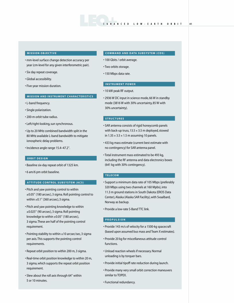
4 1LEO+E N H A N C E D . L O W - E A R T H . O R B I T 4 1LEO+

M I S S I O N O B J E C T I V E

• mm-level surface change detection accuracy per

year (cm-level for any given interferometric pair).

• Six day repeat coverage.

• Global accessibility.

• Five-year mission duration.

M I S S I O N A N D I N S T R U M E N T C H A R AC T E R I S T I C S

• L-band frequency.

• Single polarization.

• 200-m orbit tube radius.

• Left/right-looking, sun synchronous.

• Up to 20 MHz combined bandwidth split in the

80 MHz available L-band bandwidth to mitigate

ionospheric delay problems.

• Incidence angle range 15.4–47.2°.

O R B I T D E S I G N

• Baseline six-day repeat orbit of 1325 km.

• 6 am/6 pm orbit baseline.

A T T I T U D E C O N T R O L S U B S Y S T E M ( A C S )

• Pitch and yaw pointing control to within

±0.05° (180 arcsec), 3 sigma. Roll pointing control to

within ±0.1° (360 arcsec), 3 sigma.

• Pitch and yaw pointing knowledge to within

±0.025° (90 arcsec), 3 sigma. Roll pointing

knowledge to within ±0.05° (180 arcsec),

3 sigma. These are half of the pointing control

requirement.

• Pointing stability to within ±10 arcsec/sec, 3 sigma

per axis. This supports the pointing control

requirements.

• Repeat orbit position to within 200 m, 3 sigma.

• Real-time orbit position knowledge to within 20 m,

3 sigma, which supports the repeat orbit position

requirement.

• Slew about the roll axis through 64° within

5 or 10 minutes.

C O M M A N D A N D D ATA S U B S Y S T E M ( C D S )

• 100 Gbits / orbit average.

• Two orbits storage.

• 150 Mbps data rate.

I N S T R U M E N T P O W E R

• 10 kW peak RF output.

• 2936 W DC input in science mode, 66 W in standby

mode (3816 W with 30% uncertainty, 85 W with

30% uncertainty).

S T R U C T U R E S

• SAR antenna consists of rigid honeycomb panels

with back-up truss, 13.5 × 3.5 m deployed, stowed

in 1.35 × 3.5 × 1.5 m assuming 10 panels.

• 433 kg mass estimate (current best estimate with

no contingency) for SAR antenna panel.

• Total instrument mass estimated to be 493 kg,

including the RF antenna and data electronics boxes

(641 kg with 30% contingency).

T E L E C O M

• Support a minimum data rate of 105 Mbps (preferably

320 Mbps using two channels at 160 Mpbs), into

11.3 m ground stations in South Dakota (EROS Data

Center), Alaska (Alaska SAR Facility), with Svaalbard,

Norway as backup.

• Provide a low-rate S-Band TTC link.

P R O P U L S I O N

• Provide 143 m/s of velocity for a 1500-kg spacecraft

(based upon assumed bus mass and Team X estimates).

• Provide 20 kg for miscellaneous attitude control

functions.

• Unload reaction wheels if necessary. Normal

unloading is by torquer bars.

• Provide initial tipoff rate reduction during launch.

• Provide many very small orbit correction maneuvers

similar to TOPEX.

• Functional redundancy.

E N H A N C E D . L O W - E A R T H . O R B I T

G L O B A L . E A R T H Q U A K E . S A T E L L I T E . S Y S T E M4 2

Figure 3.8

System elements

for launch, flight,

and ground

operations.

CommercialSpacecraft Bus

FLIGHT SEGMENTLAUNCH SERVICES

GROUND SEGMENT

UplinkStation

Global Network ofDownlink Stations

GESS DataPlanning andManagementGESS

OperationsCenter

GESS SARData Catalogand Archive

Customers

Launch Vehicle(Delta II)

L-BandSAR Instrument

SAR DataProcessing

A survey has been completed that indicates

several manufacturers can supply satellite

busses that meet or exceed the LEO+ require-

ments with little or no modifications to exist-

ing designs. All of the busses surveyed have

substantial flight heritage and utilize space

qualified components and technologies.

Some of the available busses are production-

oriented designs that will provide substantial

cost and schedule efficiencies. The cost-saving

approach for selecting a bus for nominal de-

sign requires that the bus requires little modi-

fication, has substantial space flight heritage,

is compatible with multiple launch vehicles,

has redundancy and sufficient margins to

accommodate unexpected changes in the

designs, uses radiation-hard standard or

commercial parts when possible, and has well-

defined interfaces to allow parallel develop-

ment and testing of the instrument.

Launch Vehicle

The LEO+ launch vehicle will be obtained

by the NASA Expendable Launch Vehicle

Office and provided to the project using

NASA ELV Office procurement and quality

assurance processes. The NLS-Medium

launch vehicle (Delta II) was assumed, as it

can place the spacecraft into the desired orbit

(Figure 3.9). A Delta IV would provide ample

mass and volume margin.

Assembly, Test, and Launch Operations(AT&LO)

Once the LEO+ system design is complete

and has passed the critical design review

(CDR), production of the major elements

will proceed concurrently. The spacecraft bus,

radar instrument, and ground segment sys-

tems and their components will complete a

rigorous test program during development

and build-up for flight. All subsystems will

4 3LEO+E N H A N C E D . L O W - E A R T H . O R B I T 4 3

Figure 3.9

The LEO+ payload in

stowed configuration

in a Delta II launch

vehicle fairing.

be thoroughly tested prior to delivery to

AT&LO (Figure 3.10). The objectives are to

verify system level requirements, functional

interfaces, and nominal performance of the

integrated flight segment configuration in

flight-like conditions.

The main objectives for AT&LO are:

• Provide an integrated, test validated,

flight-ready space segment consisting of the

spacecraft bus, radar instrument, and launch

vehicle, which is capable of being launched

on the scheduled launch date.

• Plan and implement traceable, repeatable,

and comprehensible test activities.

• Demonstrate an ability to support the

spacecraft and the mission objectives with

functionally validated ground operations

and data processing systems.

The AT&LO program shall test or dem-

onstrate the following:

• Compliance of the integrated flight segment

with system-level design and functional

requirements.

• Nominal flight segment performance in

ambient and expected environmental condi-

tions (of launch and flight), with baseline

representative operational sequences; and,

predictable performance in selected

contingency conditions.

• Compatibility with the launch vehicle and

launch systems interface requirements.

• Compatibility with the ground segment

and operations systems.

• Verified spacecraft capability to receive

and process commands, and to clock out

execution time for commands or command

sequences that cannot be fully tested in

ambient/ground environments.

In addition to traditional integration and

test support, the AT&LO organization will

also support a postlaunch on-orbit commis-

sioning phase to checkout and calibrate the

end-to-end flight and ground system. The

AT&LO activity will conclude upon comple-

tion of the operational acceptance review,

which occurs at the end of the commissioning

phase.

AT & LO A p p r o a c h

The AT&LO approach targets several

areas, including the early use of a system

testbed to evaluate and confirm avionics

architecture and end-to-end Information

System design in order to avoid surprises

and risks later in integration and testing

(I&T). The spacecraft bus manufacturer will

be responsible for the spacecraft bus I&T,

and will deliver a fully integrated and tested

bus. The radar system I&T would follow the

incremental build and test approach. Final

flight element I&T would be conducted at

the spacecraft bus contractor facility. No

thermal/vacuum tests at system level, no post-

environmental antenna deployment test, and

only limited mechanical/integrity verifications

G L O B A L . E A R T H Q U A K E . S A T E L L I T E . S Y S T E M4 4

Figure 3.10

Satellite

integration and

test flow.

Integrate SubsystemsAmbient Electrical Test

Initial Mass Properties,Alignments

Initial Environmental:EMC, Vibe, Thermal

Assemble/IntegrateSubsystems & Structure

Install Solar Arraysand Deployables

Vibration and Acoustic Testing

Install Solar Arraysand Deployables

Comprehensive System Test:Electrical, Thermal Cycling

ComprehensiveSystem Test

Slow DeployablesTest

Launch ConfigurationThermal Vacuum Test

ComprehensiveSystem Test

Integrate RadarInstrument

JPL DeliversRadar Instrument

Remove Solar Arrayand Deployables

Package and Shipto Launch Site

Launch Site Activities• Final Assembly and Inspection

• Final Functional Testing• Launcher Mating

• Fueling

SUBSYSTEM LEVEL

SYSTEM LEVEL

are assumed. There will be maximum use of

system engineering in other WBS elements.

The launch will be from the Western Test

Range (Vandenberg Air Force Base).

Ground Data System and Produc ts

The GESS Ground Data System (GDS) is

designed to support the disaster management

community (Figure 3.8). Specifically, the data

latency for disaster response is two hours or

less for time-tagged raw data and six hours

or less for Level 1 data products, which could

be utilized directly by the disaster response

teams. Two downlink stations are planned to

capture all the raw data being acquired, the

EROS Data Center (EDC) in South Dakota

and the Alaska SAR Facility (ASF). The

Svaalbard Ground Station in Norway will

serve as a backup downlink station. EDC

would be the central data archiving and pro-

cessing center, whereas another center, such

as JPL, would serve as the GDS development

site and backup data archiving and processing

facility. JPL would have the capability to

handle both the standard data product deliv-

ery as well as special event product generation.

Level 0 product generation may be done at

the downlink station and transmitted directly

to the users when needed to reduce the data

transmission overhead via EDC.

In the following section, we will summarize

the ground data system requirements and cor-

responding design impact on the GDS for the

LEO+ mission. We will describe the output

products based on inputs from the seismology

community. Next, we describe the external in-

terfaces to the GDS and the distributed soft-

ware architecture. The distributed nature and

4 5LEO+E N H A N C E D . L O W - E A R T H . O R B I T 4 5

scalability of the GDS architecture designed

for the LEO+ mission can be easily expanded

to support a geosynchronous mission. We de-

scribe the hardware architecture of the GDS,

which is composed entirely of commercial

off-the-shelf (COTS) products.

G r o u n d D a t a Sy s t e m R e q u i r e m e n t s

Based on the functional requirements for

the LEO+ mission, the ground data system

requirements and design impacts are summa-

rized in Table 3.4.

D a t a P r o d u c t D e f i n i t i o n s

Two primary user communities with differ-

ent requirements will be supported: those with

radar processing capabilities, and researchers

relying on geophysical Level 2 products. The

former group of users would request the raw

radar data to process themselves. In addition,

they will need ancillary data for the purpose of

calibration such as the removal of atmospheric

effects. The second group of researchers who

have no interest or capability to process their

own radar data prefer to work directly with

the geo-coded differential interferograms

to extract the deformation measurements.

Therefore, as shown in Table 3.5, the data

products are defined to serve both of these

user communities.

All level data products have accompanying

metadata, which includes the ancillary data

and quality, calibration, and processing param-

eters. Quick-look data (without corrections)

will also be available. Ancillary data needed

for processing includes:

• Satellite orbit information derived from

onboard GPS

• Ground reference GPS (from mission

operations)

• Atmospheric path delay model (from meteo-

rological services)

• Ground truth data (from external sources)

necessary for calibration

Browse products will be generated for all

Level 1a, 1b, and 2 products. Ancillary data

may be bundled with any level data product

delivery.

G r o u n d D a t a S y s t e m I n t e r f a c e s

The GESS GDS is an integrated SAR

processing, product delivery, and archiving

system. The GDS interfaces with the follow-

ing components:

• Spacecraft operations

• Science users

• Program management

• Algorithm developers and calibration

engineers

• Ancillary data sources

The high-level GDS boundaries and

external interfaces are shown in Figure 3.11.

Spacecraft operations provide satellite-task-

ing information (instrument on/off times and

modes) to the GDS. This information is cata-

logued, used for internal processing and made

available via a Web-based GIS interface (inter-

active map) and subscription. It also provides

ground station tasking and downlinked data.

Science users access the GDS through a Web

portal. This portal provides product and pro-

cessing request capability, as well as other fea-

tures such as data mining and education and

outreach. Program management accesses the

GDS through a Web portal to view metrics

and provide processing priorities etc. Algo-

rithm developers submit basic algorithms and

refinements through a Web-enabled configu-

ration management interface. The GDS

actively acquires and ingests ancillary files

required for product processing.

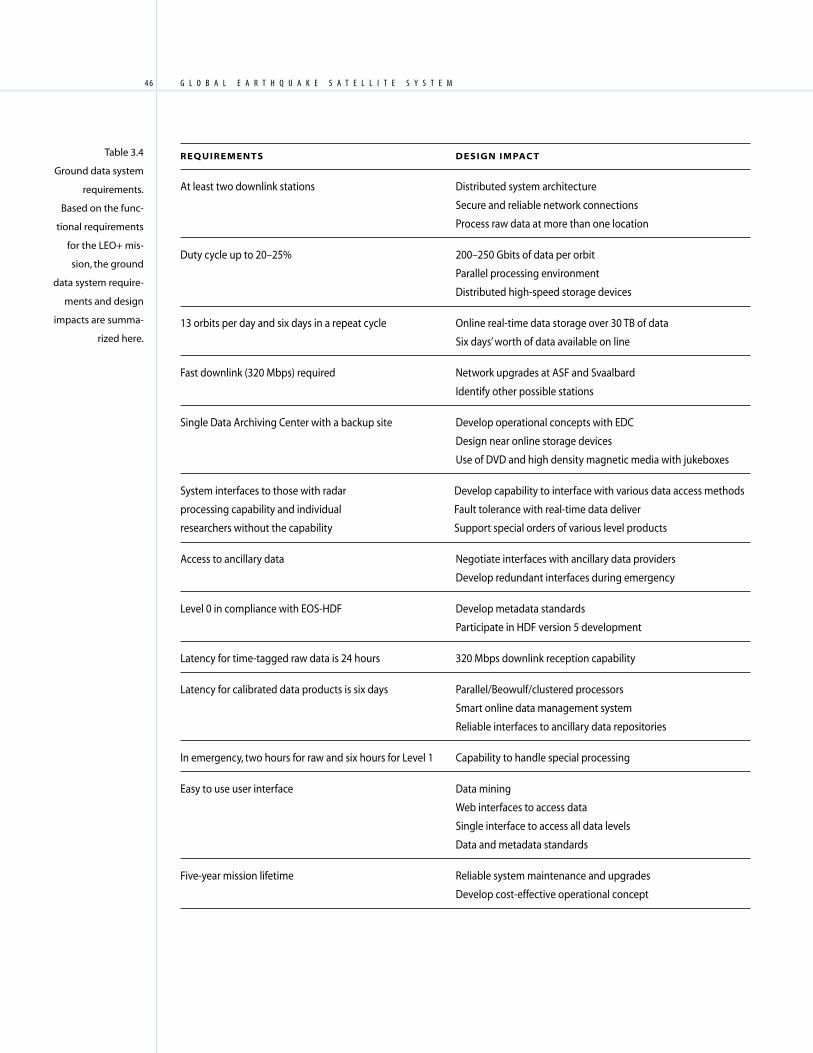
G L O B A L . E A R T H Q U A K E . S A T E L L I T E . S Y S T E M4 6

Table 3.4

Ground data system

requirements.

Based on the func-

tional requirements

for the LEO+ mis-

sion, the ground

data system require-

ments and design

impacts are summa-

rized here.

REQUIREMENTS DESIGN IMPACT

At least two downlink stations Distributed system architecture

Secure and reliable network connections

Process raw data at more than one location

Duty cycle up to 20–25% 200–250 Gbits of data per orbit

Parallel processing environment

Distributed high-speed storage devices

13 orbits per day and six days in a repeat cycle Online real-time data storage over 30 TB of data

Six days’ worth of data available on line

Fast downlink (320 Mbps) required Network upgrades at ASF and Svaalbard

Identify other possible stations

Single Data Archiving Center with a backup site Develop operational concepts with EDC

Design near online storage devices

Use of DVD and high density magnetic media with jukeboxes

System interfaces to those with radar Develop capability to interface with various data access methods

processing capability and individual Fault tolerance with real-time data deliver

researchers without the capability Support special orders of various level products

Access to ancillary data Negotiate interfaces with ancillary data providers

Develop redundant interfaces during emergency

Level 0 in compliance with EOS-HDF Develop metadata standards

Participate in HDF version 5 development

Latency for time-tagged raw data is 24 hours 320 Mbps downlink reception capability

Latency for calibrated data products is six days Parallel/Beowulf/clustered processors

Smart online data management system

Reliable interfaces to ancillary data repositories

In emergency, two hours for raw and six hours for Level 1 Capability to handle special processing

Easy to use user interface Data mining

Web interfaces to access data

Single interface to access all data levels

Data and metadata standards

Five-year mission lifetime Reliable system maintenance and upgrades

Develop cost-effective operational concept

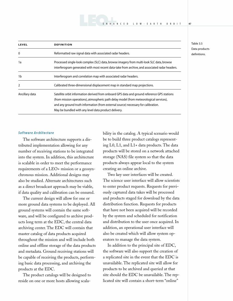
4 7LEO+E N H A N C E D . L O W - E A R T H . O R B I T 4 7

Table 3.5

Data products

definitions.

LEVEL D EFINITION

0 Reformatted raw signal data with associated radar headers.

1a Processed single-look complex (SLC) data, browse imagery from multi-look SLC data, browse

interferogram generated with most recent data-take from archive, and associated radar headers.

1b Interferogram and correlation map with associated radar headers.

2 Calibrated three-dimensional displacement map in standard map projections.

Ancillary data Satellite orbit information derived from onboard GPS data and ground reference GPS stations

(from mission operations), atmospheric path delay model (from meteorological services),

and any ground truth information (from external source) necessary for calibration.

May be bundled with any level data product delivery.

S o f t wa r e A r c h i t e c t u r e

The software architecture supports a dis-

tributed implementation allowing for any

number of receiving stations to be integrated

into the system. In addition, this architecture

is scalable in order to meet the performance

requirements of a LEO+ mission or a geosyn-

chronous mission. Additional designs may

also be studied. Alternate architectures such

as a direct broadcast approach may be viable,

if data quality and calibration can be ensured.

The current design will allow for one or

more ground data systems to be deployed. All

ground systems will contain the same soft-

ware, and will be configured to archive prod-

ucts long term at the EDC, the central data

archiving center. The EDC will contain that

master catalog of data products acquired

throughout the mission and will include both

online and offline storage of the data products

and metadata. Ground receiving stations will

be capable of receiving the products, perform-

ing basic data processing, and archiving the

products at the EDC.

The product catalogs will be designed to

reside on one or more hosts allowing scala-

bility in the catalog. A typical scenario would

be to build three product catalogs represent-

ing L0, L1, and L1+ data products. The data

products will be stored on a network attached

storage (NAS) file system so that the data

products always appear local to the system

creating an online archive.

Two key user interfaces will be created.

The science user interface will allow scientists

to enter product requests. Requests for previ-

ously captured data takes will be processed

and products staged for download by the data

distribution function. Requests for products

that have not been acquired will be recorded

by the system and scheduled for notification

and distribution to the user once acquired. In

addition, an operational user interface will

also be created which will allow system op-

erators to manage the data system.

In addition to the principal site of EDC,

the software will also support the creation of

a replicated site in the event that the EDC is

unavailable. The replicated site will allow for

products to be archived and queried at that

site should the EDC be unavailable. The rep-

licated site will contain a short-term “online”

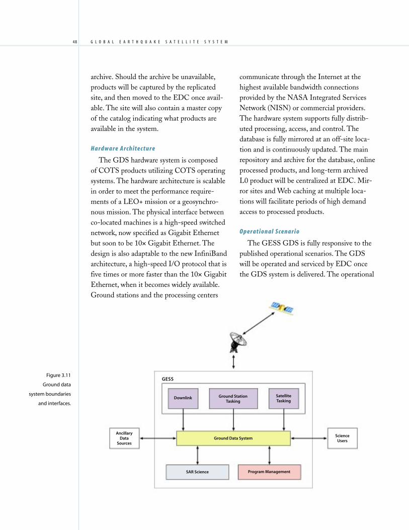
G L O B A L . E A R T H Q U A K E . S A T E L L I T E . S Y S T E M4 8

Figure 3.11

Ground data

system boundaries

and interfaces.

GESS

Downlink Ground StationTasking

SatelliteTasking

Ground Data System

SAR Science Program Management

AncillaryData

Sources

ScienceUsers

archive. Should the archive be unavailable,

products will be captured by the replicated

site, and then moved to the EDC once avail-

able. The site will also contain a master copy

of the catalog indicating what products are

available in the system.

H a r d w a r e A r c h i t e c t u r e

The GDS hardware system is composed

of COTS products utilizing COTS operating

systems. The hardware architecture is scalable

in order to meet the performance require-

ments of a LEO+ mission or a geosynchro-

nous mission. The physical interface between

co-located machines is a high-speed switched

network, now specified as Gigabit Ethernet

but soon to be 10× Gigabit Ethernet. The

design is also adaptable to the new InfiniBand

architecture, a high-speed I/O protocol that is

five times or more faster than the 10× Gigabit

Ethernet, when it becomes widely available.

Ground stations and the processing centers

communicate through the Internet at the

highest available bandwidth connections

provided by the NASA Integrated Services

Network (NISN) or commercial providers.

The hardware system supports fully distrib-

uted processing, access, and control. The

database is fully mirrored at an off-site loca-

tion and is continuously updated. The main

repository and archive for the database, online

processed products, and long-term archived

L0 product will be centralized at EDC. Mir-

ror sites and Web caching at multiple loca-

tions will facilitate periods of high demand

access to processed products.

O p e r a t i o n a l S c e n a r i o

The GESS GDS is fully responsive to the

published operational scenarios. The GDS

will be operated and serviced by EDC once

the GDS system is delivered. The operational

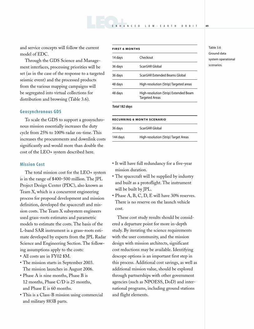
4 9LEO+E N H A N C E D . L O W - E A R T H . O R B I T 4 9

Table 3.6

Ground data

system operational

scenarios.

F I R S T 6 M O N T H S

14 days Checkout

36 days ScanSAR Global

36 days ScanSAR Extended Beams Global

48 days High-resolution (Strip) Targeted areas

48 days High-resolution (Strip) Extended BeamTargeted Areas

Total 182 days

R E C U R R I N G 6 M O N T H S C E N A R I O

36 days ScanSAR Global

144 days High-resolution (Strip) Target Areas

and service concepts will follow the current

model of EDC.

Through the GDS Science and Manage-

ment interfaces, processing priorities will be

set (as in the case of the response to a targeted

seismic event) and the processed products

from the various mapping campaigns will

be segregated into virtual collections for

distribution and browsing (Table 3.6).

Geosynchronous GDS

To scale the GDS to support a geosynchro-

nous mission essentially increases the duty

cycle from 25% to 100% radar on-time. This

increases the procurements and downlink costs

significantly and would more than double the

cost of the LEO+ system described here.

Mission Cost

The total mission cost for the LEO+ system

is in the range of $400–500 million. The JPL

Project Design Center (PDC), also known as

Team X, which is a concurrent engineering

process for proposal development and mission

definition, developed the spacecraft and mis-

sion costs. The Team X subsystem engineers

used grass-roots estimates and parametric

models to estimate the costs. The basis of the

L-band SAR instrument is a grass-roots esti-

mate developed by experts from the JPL Radar

Science and Engineering Section. The follow-

ing assumptions apply to the costs:

• All costs are in FY02 $M.

• The mission starts in September 2003.

The mission launches in August 2006.

• Phase A is nine months, Phase B is

12 months, Phase C/D is 25 months,

and Phase E is 60 months.

• This is a Class-B mission using commercial

and military 883B parts.

• It will have full redundancy for a five-year

mission duration.

• The spacecraft will be supplied by industry

and built as a protoflight. The instrument

will be built by JPL.

• Phase A, B, C, D, E will have 30% reserves.

There is no reserve on the launch vehicle

cost.

These cost study results should be consid-

ered a departure point for more in-depth

study. By iterating the science requirements

with the user community, and the mission

design with mission architects, significant

cost reductions may be available. Identifying

descope options is an important first step in

this process. Additional cost savings, as well as

additional mission value, should be explored

through partnerships with other government

agencies (such as NPOESS, DoD) and inter-

national programs, including ground stations

and flight elements.

G L O B A L . E A R T H Q U A K E . S A T E L L I T E . S Y S T E M5 0

Geosynchronous Architecture

C H A P T E R

F O U R

he most ambitious concept of the GESS study entails the operation of a

geosynchronous SAR constellation. While the deployment of such a constella-

tion would be a massive undertaking and require that major technological

challenges be overcome, a constellation of high-altitude SAR satellites would

offer advantages over lower-altitude sensors in the contexts of system

operational flexibility and instantaneous accessibility of target areas on the

ground (Figure 4.1). A system with such capabilities might be considered as

a mission for the next decade.

Geosynchronous orbits are unique because their orbital periods are equal

to one Earth day. A geostationary orbit is a special kind of geosynchronous

orbit in which the orbital inclination is zero; viewed from the rotating Earth, a

satellite in a geostationary orbit appears to remain fixed in the same position

in the sky at all times. This property makes geostationary orbits ideal for such

applications as communications and meteorology, but it in fact makes them

unusable for SAR missions. This is because the principle of aperture synthesis

— the very principle for which SAR is named — requires relative motion

between the sensor and the scene under observation. When such motion

exists, as it does for an inclined geosynchronous orbit, however, fine resolu-

tion can be obtained even from very great distances. Although a geosynchro-

nous satellite follows an elliptical trajectory as dictated by Kepler’s laws of

motion, due to the relative motion of the Earth and the satellite, the nadir

point traces out a “figure-8” pattern on the ground once per day (see Figure

4.2). Since radar instruments can also acquire images both during the day and

at night, and unaffected by cloud cover, a high-altitude SAR constellation may

be well suited to the task of 24-hour global hazard monitoring. Most of the

Earth’s surface could be kept in view nearly continuously by a constellation

of geosynchronous satellites.

T

5 1

System Parameters

A geosynchronous SAR at an altitude of

about 35,800 km would be more than an or-

der of magnitude farther from the Earth than

any SAR mission to date. While this high-

altitude vantage point would allow a geosyn-

chronous SAR to view a large ground area, it

would also require a large physical antenna

and a great deal of transmitted power. The

antenna size requirements are driven by the

need to resolve the range-Doppler ambigu-

ities that are inherent in a pulsed radar sys-

tem; the power requirements are driven by

signal-to-noise ratio (SNR) considerations.

We envision a system with a 30-m-diam-

eter L-band aperture antenna that transmits

60 kW of peak power over relatively long

1-ms pulses. The boresight of this antenna

would be kept pointed in the nadir direction

and the beam steered electronically to look

either left or right. Any part of the sensor

footprint could be illuminated with no more

than ±8° of electronic steering — from this

altitude, the limb of the Earth is only 9° from

nadir. Data could therefore be acquired for

areas between 1000 and 6500 km ground

range from nadir on either side of the plat-

form ground track, corresponding to ground-

incidence angles of 10.6–66.4°. The antenna

could also be steered to areas with ground

squint angles up to ±60° on either side of the

ground track with less than ±8° of electronic

steering in the azimuth direction.

With such a wide swath, some of the sys-

tem parameters would have to change a great

deal between the near range and the far range.

The bandwidth of the system might vary

between 80 MHz at the steepest incidence

angles to 10 MHz further out. A split-spec-

trum approach might be employed as in the

LEO+ case in order to characterize the effects

of the ionosphere. The signal polarization

might also change over the sensor footprint.

We envision that the spacecraft would be

yaw steered to keep the antenna in a nominal

HH polarization state for broadside acquisi-

tion geometries, implying that the polariza-

tion state would be mixed in squinted

geometries.

Figure 4.1

Cumulative land

coverage from both

LEO+ and GEO

constellations of

three satellites. The

GEO constellation

achieves over 90%

land coverage in

approximately half

the time of the

LEO+ constellation.

GEOG E O S Y N C H R O N O U S . A R C H I T E C T U R E

100

90

80

70

60

50

40

30

20

10

0

3 6 9 12 15 18 21 24

3 LEO+3 Geosynchronous

Perc

ent

Cu

mu

lati

ve L

and

Co

vera

ge

Time (hours)

G L O B A L . E A R T H Q U A K E . S A T E L L I T E . S Y S T E M5 2

Other system parameters would change

over the platform orbit as the velocity of the

platform relative to an observer on the Earth

varies. For an orbital inclination of 60°, the

relative velocity of the satellite would vary by

a factor of two between about 1500 m/s when

the satellite is at high latitudes and 3000 m/s

when it is over the equator. The pulse repeti-

tion frequency (PRF) of the system would

therefore vary between about 125 Hz and

250 Hz. Relevant system parameters are sum-

marized in Table 4.1. Note that these relative

velocities and PRFs are significantly lower

than those of LEO systems.

Orbit, Coverage, Constellation

Although a geosynchronous SAR would

have a very large footprint, its “figure-8”

ground track would always remain in a fixed

set of longitudes. A single geosynchronous

sensor would consequently be unable to pro-

vide global coverage on its own. While the

longitude-locked behavior of a geosynchro-

nous SAR might prove advantageous if the

mission objective were to provide coverage

only of the Western hemisphere, the aim

of this study has been the development of

system whose scope is global. Consequently,

we concentrate here on the use of multiple

geosynchronous sensors.

One architecture would be a constellation

of ten satellites divided into five groups of two

(Figure 4.3). The two satellites in each group

would follow the same ground track and

would be phased 180° apart, resulting in an

interferometric repeat time of 12 hours. In

Figure 4.2

Trace of a geosyn-

chronous satellite

at a 60° orbit incli-

nation (shown as

figure-8). Instanta-

neous field of view

for a 5500-km SAR

swath is also shown.

5 3GEOG E O S Y N C H R O N O U S . A R C H I T E C T U R E

Table 4.1

Geosynchronous

parameters.

ORBIT

Altitude 35788 km

Inclination 60°

Interferometric Repeat Period 1 day

VI SI BLE SWAT H

Look Angle ± 1.6–8.0°

Ground Incidence Angle ±10.6–66.4°

Ground Range From Nadir ±1000–6500 km

Slant Range 35892–39224 km

Ground Squint Angle ±60°

Footprint Area 79,000,000 km2

Subswath Width 400 km nominal

I N S T RU M E N T

Antenna Diameter 30 m

Electronic Steering ±8° in azimuth and elevation

Wavelength 24 cm (L-band)

Polarization varies with squint angle

Peak Transmit Power 60 kW

Pulse Duration 1 ms

Bandwidth 10–80 MHz

Pulse Repetition Frequency 125–250 Hz

P E R F O R M A N C E

Ground Range Resolution 20 m nominal

Stripmap Azimuth Resolution varies over orbit (2–20 m nominal)

Nominal SNR 10 dB

Nominal Range Ambiguity Level –30 dB

Nominal Azimuth Ambiguity Level –20 dB

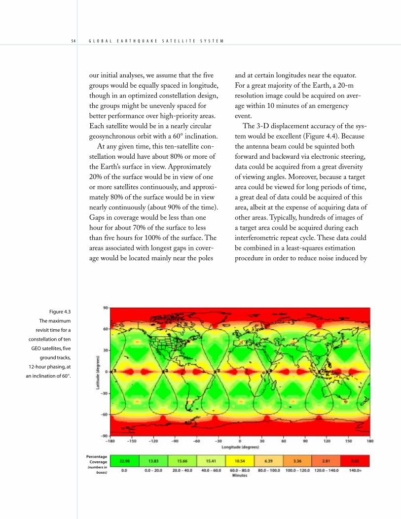
G L O B A L . E A R T H Q U A K E . S A T E L L I T E . S Y S T E M5 4

our initial analyses, we assume that the five

groups would be equally spaced in longitude,

though in an optimized constellation design,

the groups might be unevenly spaced for

better performance over high-priority areas.

Each satellite would be in a nearly circular

geosynchronous orbit with a 60° inclination.

At any given time, this ten-satellite con-

stellation would have about 80% or more of

the Earth’s surface in view. Approximately

20% of the surface would be in view of one

or more satellites continuously, and approxi-

mately 80% of the surface would be in view

nearly continuously (about 90% of the time).

Gaps in coverage would be less than one

hour for about 70% of the surface to less

than five hours for 100% of the surface. The

areas associated with longest gaps in cover-

age would be located mainly near the poles

and at certain longitudes near the equator.

For a great majority of the Earth, a 20-m

resolution image could be acquired on aver-

age within 10 minutes of an emergency

event.

The 3-D displacement accuracy of the sys-

tem would be excellent (Figure 4.4). Because

the antenna beam could be squinted both

forward and backward via electronic steering,

data could be acquired from a great diversity

of viewing angles. Moreover, because a target

area could be viewed for long periods of time,

a great deal of data could be acquired of this

area, albeit at the expense of acquiring data of

other areas. Typically, hundreds of images of

a target area could be acquired during each

interferometric repeat cycle. These data could

be combined in a least-squares estimation

procedure in order to reduce noise induced by

Figure 4.3

The maximum

revisit time for a

constellation of ten

GEO satellites, five

ground tracks,

12-hour phasing, at

an inclination of 60°.

PercentageCoverage

(numbers in

boxes)

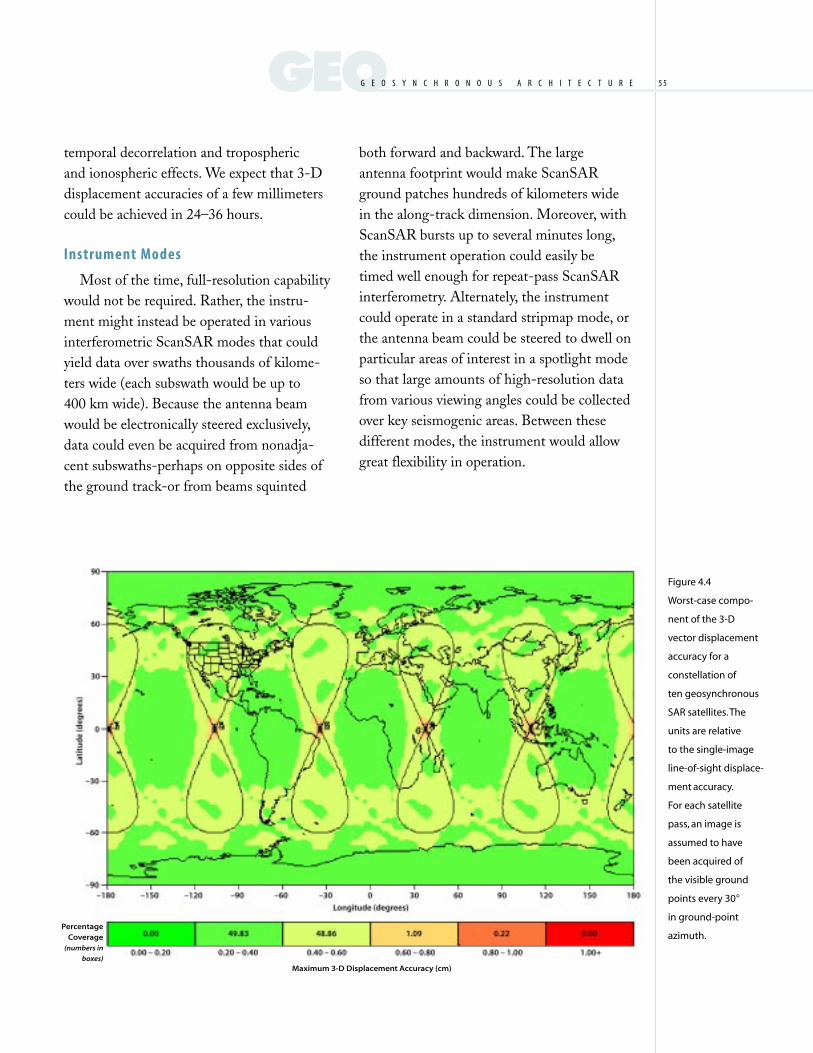
5 5GEO

Figure 4.4

Worst-case compo-

nent of the 3-D

vector displacement

accuracy for a

constellation of

ten geosynchronous

SAR satellites. The

units are relative

to the single-image

line-of-sight displace-

ment accuracy.

For each satellite

pass, an image is

assumed to have

been acquired of

the visible ground

points every 30°

in ground-point

azimuth.

temporal decorrelation and tropospheric

and ionospheric effects. We expect that 3-D

displacement accuracies of a few millimeters

could be achieved in 24–36 hours.

Instrument Modes

Most of the time, full-resolution capability

would not be required. Rather, the instru-

ment might instead be operated in various

interferometric ScanSAR modes that could

yield data over swaths thousands of kilome-

ters wide (each subswath would be up to

400 km wide). Because the antenna beam

would be electronically steered exclusively,

data could even be acquired from nonadja-

cent subswaths-perhaps on opposite sides of

the ground track-or from beams squinted

both forward and backward. The large

antenna footprint would make ScanSAR

ground patches hundreds of kilometers wide

in the along-track dimension. Moreover, with

ScanSAR bursts up to several minutes long,

the instrument operation could easily be

timed well enough for repeat-pass ScanSAR

interferometry. Alternately, the instrument

could operate in a standard stripmap mode, or

the antenna beam could be steered to dwell on

particular areas of interest in a spotlight mode

so that large amounts of high-resolution data

from various viewing angles could be collected

over key seismogenic areas. Between these

different modes, the instrument would allow

great flexibility in operation.

Maximum 3-D Displacement Accuracy (cm)

PercentageCoverage

(numbers in

boxes)

G E O S Y N C H R O N O U S . A R C H I T E C T U R E

G L O B A L . E A R T H Q U A K E . S A T E L L I T E . S Y S T E M5 6

The system might have numerous modes

that are tailored to different situations and

changing priorities. A typical operational

plan might involve the daily or twice-daily

creation of multiple maps of certain high-

priority seismogenic areas (as described in

the LEO+ scenario) as well as low-resolu-

tion global maps every few days, or high-

resolution global maps every few weeks. The

operational plan could also be modified as

needed in response to global hazard events

and current conditions.

Per formance

Because the curvature of the relative plat-

form motion changes a great deal over the

orbit, the stripmap-mode azimuth resolu-

tion depends on the satellite latitude and

location of the target in the sensor footprint.

When the instrument is looking towards

the outside of each loop in the figure-8 pat-

tern, the stripmap-mode azimuth resolution

can be as coarse as 20 m, yet it can be finer

than 2 m when the instrument is looking

towards the inside. That is, in some cases,

the orbit curvature would effectively cause

the antenna beam to dwell on a particular

ground area in a manner similar to that of a

spotlight-mode SAR acquisition, even when

the antenna beam is kept pointing toward

broadside. Azimuth resolutions of around

2 m or better might also be obtained any-

where in the swath or along the orbit when

the instrument is operating explicitly in

spotlight mode.

The processing involved for attaining

2-m resolution would not be trivial, how-

ever. The required synthetic aperture length

for such a resolution would be more than

200 km, over which the curvature of the

platform motion would change significantly.

In fact, a different azimuth-compression

reference function would be required for

each along-track sample position. Moreover,

the slant-range depth of focus might be

even smaller than the nominal slant-range

resolution of around 10–20 m if 2-m resolu-

tion is desired. Another difficulty of high-

resolution processing would be posed by the

variability of the ground scene and of the

atmosphere over the time required by the

satellite to traverse the long synthetic aper-

ture distances; up to 25 min may be required

in some situations. In practice, 2-m resolu-

tion may be very difficult to achieve, though

5–10-m azimuth resolutions should be

readily attainable. Note that while fine

spatial resolution is not always required for

geophysical applications, high-resolution

data can be averaged spatially in order to

mitigate the effects of temporal

decorrelation in interferometric data.

Indeed, as in the LEO+ case, we expect

that the interferometric displacement accu-

racy will be limited more by temporal de-

correlation as well as by tropospheric or

ionospheric effects than by the instrument

performance. Given the large amount of

data that a geosynchronous system can

acquire of a targeted area over a short period

of time, though, it is not unreasonable to

expect that with sufficient averaging, the

displacement accuracy can be reduced to the

level of a few millimeters for specific target

sites. Over larger areas, we expect that

subcentimeter displacement accuracies

would be typical.

The instrument would also allow for

excellent 3-D displacement accuracy over

much of the Earth since most points on the

ground could be imaged from diverse sets of

5 7

viewing angles. This diversity of viewing

angles comes from the both the lateral curva-

ture of the ground track as well as the varia-

tion in ground squint angles that are possible

through electronic beam steering from high

altitudes.

Data Rates and Volume

Although the footprint of a geosynchro-

nous SAR’s accessible area would be much

larger than that of a sensor in a lower orbit,

the instantaneous data rates of the two would

be comparable (on the order of 100–200 Mbs).

This is because neither sensor would be able

to acquire full-resolution data over its entire

footprint simultaneously; data would need to

be collected over smaller subswaths. While

the subswaths of a geosynchronous SAR

would be considerably wider than those of a

LEO SAR, the Earth-relative velocity is

slower. Despite comparable data rates, because

the geosynchronous sensor is almost always in

sight of land, even when the sensor itself is

over water, the instrument could acquire data

nearly continuously. The total data volume

could therefore be on the order of 1–2 TB per

satellite per day, or around 5–10 PB per satel-

lite over the satellite’s relatively long 15-year

life. These values would increase by a factor

of two or four if multiple radar polarizations

were used.

Such data rates and volumes would require

specialized downlink and data-handling facili-

ties. Since geosynchronous satellites would

be in view continuously from low-latitude

ground stations for long periods of time, how-

ever, one or two dedicated ground stations

could be used to downlink the data from each

satellite or each pair of satellites in the same

ground track. Furthermore, with appropriate

intersatellite communication, one or two

ground stations might be able to handle all

of the data from an entire constellation.

Geosynchronous SAR PayloadDescription

The geosynchronous SAR instrument is

dominated by the very large deployable an-

tenna. Because of the large antenna area, our

mission concept integrates the SAR antenna

with the spacecraft structure and subsystems

as illustrated in Figure 4.5. The 30-m-diam-

eter antenna aperture is deployed with

horizontal booms and then tensioned to

maintain flatness with two asymmetric axi-

ally deployed masts and tensioning cables.

The antenna aperture is constructed from

flexible membrane material that is integrated

with the active electronics for proper beam

formation and transmit/receive signal ampli-

fication. The antenna flatness must be main-

tained to within 1/20 of a wavelength, or

roughly 1 cm across the entire aperture. This

type of flatness requirement can be achieved

using the axial booms and membrane

tensioning cables.

Due to the challenge of such a flatness

requirement, the proper calibration of the

full array is essential for successful beam-

forming. The principal array error sources

include feed errors caused by variations

in electronic components, and element

displacement caused by mechanical defor-

mation of the array surface. The removal

of displacement errors is somewhat prob-

lematic. Only an external calibration system

can address the problem of element dis-

placement. There is a trade-off between

mechanical rigidity (and thus, surface accu-

racy) and mass. In order to minimize the

launch mass, it is desirable to tolerate greater

GEOG E O S Y N C H R O N O U S . A R C H I T E C T U R E

G L O B A L . E A R T H Q U A K E . S A T E L L I T E . S Y S T E M5 8

surface errors. The added complexity of an

external calibration system must be weighed

against the benefit of lighter structural

elements. There are several approaches to

external calibration. An onboard metrology

system (either optical or RF) can be used.

Feed errors include all (manufacturing, ther-

mal or aging related) amplitude and phase

errors in feed networks, interconnects and

T/R modules. There are several proven ap-

proaches to compensating for feed errors

using loop-back calibration loops. If the

feedback paths are properly designed to

eliminate leakage from adjacent elements,

this calibration can be performed continu-

ously during normal radar operation.

Thin-film solar arrays provide power to

the antenna and spacecraft. These arrays are

an integral part of the system configuration

and share the same structural elements. One

solar array is an annular ring formed around

the perimeter of the radar antenna aperture.

Solar arrays also partially cover the rear or

zenith-pointed side of the spacecraft,

stretching up the tensioning cables as shown

in Figure 4.5. The solar array “tent configu-

ration” provides a large surface area for solar

power collection from any sun orientation

but will also result in high solar pressure on

the solar arrays making station keeping more

challenging and costly. To minimize the ef-

fect, we have lengthened the axial boom for

steeper angles of the rear-facing solar array.

We have also reduced the size of the solar

arrays as much as possible. The top of the

solar array “tent” is open because the thermal

subsystem requires a window to space for

radiating excess thermal energy. The power

system also includes sufficient batteries to

operate for short periods in eclipse. On the

tips of each mast are propulsion modules for

orbit maintenance. The antenna is mounted

Figure 4.5

Geosynchronous

SAR large deployable

antenna concept.

Horizontal Booms(x 12)

Telescoping Booms(x 2)

Propulsion Modules(× 2)

L-band RF MembraneAntenna Aperture

Thin-FilmSolar Arrays

Selected Subsystemsof Spacecraft Bus

Pre-tensionedCables (x 24)

5 9GEOG E O S Y N C H R O N O U S . A R C H I T E C T U R E

to a centralized spacecraft bus that also

houses the radar central processor/controller.

The high-radiation environment of the

geosynchronous orbit poses a substantial risk

to the SAR electronics, and degrades the

performance and reliability of the solar ar-

rays. Long-term exposure can cause device

threshold shifts, increased power consump-

tion, and device damage. Radiation-hard-

ened devices and shielding can mitigate total

dose effects. The expected total dose for a

15-year mission behind 30 mils of aluminum

is 15 Mrad for a geosynchronous orbit in-

clined to 60°. Clearly, this presents a major

technical challenge. The total dose decreases

exponentially with shielding, and therefore

the expected total dose behind 100 mils of

aluminum is reduced to 600 krad. This be-

comes a more manageable problem. How-

ever, only limited shielding can be employed

for the electronics on the antenna. Greater

levels of shielding will be very massive and

bulky, and perhaps not compatible with

membrane antenna technology. Therefore,

we consider the radiation environment to be

one of the biggest challenges to realizing

this system.

A more detailed description of the radar

system architecture and antenna design will

be presented in Chapter 6. The spacecraft

bus contains the subsystems required

to perform all spacecraft housekeeping func-

tions and radar control and data handling

functions. The bus also supports the

deployable booms, masts, antenna aperture,

and solar arrays. Twelve horizontal booms

deploy, support, and tension the antenna

aperture and solar array. These booms each

have a fully deployed length of 19 m and are

supported by, as well as stowed for launch in,

the spacecraft bus. Self-rigidizable spring-

tape-reinforced (STR) inflatable booms

of 10 inches (0.25 m) in diameter were

selected as the baseline booms. Two high-

stiffness, telescoping Able Deployable

Articulated Masts (ADAM) developed by

AEC-Able provide axial support for the

large antenna and solar arrays. The masts

will be deployed axially from the top and

the bottom of the spacecraft bus. The masts

are asymmetric; the nadir-pointing mast

has a fully deployed length of 19 m and the

upper mast used to support the solar arrays

has a length of 38 m. This configuration

was chosen to maximize solar array effi-

ciency and to reduce mass and solar pres-

sure effects. Each ADAM mast has a linear

mass density of 1.3 kg/m and is stowed in a

dedicated canister for launch. The canister

for stowing the upper ADAM mast also

acts as the central mandrel for packing the

antenna aperture. This means that the

membrane aperture will be wrapped around

the upper canister for launch. The antenna

aperture is formed by three layers of thin-

film membranes. The 30-m-diameter mem-

brane antenna aperture is integrated with

all of the distributed transmit, receive, and

control electronics including T/R modules,

true-time-delay (TTD) digital transceivers,

power converters, and signal-distribution

and interconnect technologies. Twenty-four

pre-tensioned cables are used to stiffen the

horizontal booms. The upper ADAM mast

supports 12 of these cables, and the lower

ADAM mast supports the other 12 cables.

The solar arrays that provide all power for

the instrument and spacecraft housekeeping

functions are made with flexible, amorphous

thin-film technology that is 13% efficient.

The areal mass density of these solar arrays

G L O B A L . E A R T H Q U A K E . S A T E L L I T E . S Y S T E M6 0

is assumed to be about 0.63 kg/m2. The

front annular-ring-shaped solar array will

be packaged for launch and deployed in

space together with the membrane antenna

aperture. The rear arrays will be deployed

and supported by the 12 upper cables. Two

propulsion modules are located at the tips

of the ADAM masts. Each propulsion

platform consists of hydrazine thrusters,

solar-electric ion propulsion engines, and

supporting elements of the propulsion sub-

system.

The total dry mass of the integrated geo-

synchronous SAR flight system is roughly

4500 kg (with contingency). A breakdown

of mass and power is provided in Table 4.2.

The geosynchronous SAR integrated

flight system will be packaged for launch as

shown in Figure 4.6. The total launch stack

height is 8 m, which will fit in a Delta IV

fairing. The large antenna must be stowable

with high packaging-efficiency in order to

physically fit into the spacecraft launch ve-

hicle. Since low mass and low stow-volume

are driving requirements, a flexible mem-

brane antenna architecture was selected.

Rigid honeycomb panels, such as that used

for SIR-C and SRTM antennas, were not

considered due to their larger mass and

stowage volume.

Mission Design

Because of the large area of the antenna,

our concept of the mission involves the inte-

gration of the antenna and the spacecraft

structure as just described, with rigidizable

booms, deployed radially as illustrated in

Figure 4.7. An alternative, more-traditional

design involving a separate articulated solar

array was examined but not selected because

of the mechanical problems involved. The

solar arrays of the current working design are

sized such that sufficient power would be

available regardless of the satellite orienta-

tion with respect to the Sun. The spacecraft

would also carry enough battery capacity for

three minutes of instrument operation dur-

ing eclipse. This would allow images with

azimuth resolutions of 10 m or better to be

obtained in emergency situations if necessary.

Eclipses would occur once per day during

each of two month-long seasons per year,

with eclipses of up to 70 minutes duration.

The large central opening in the solar arrays

over the back of the radar antenna aperture is

required for the radiators that would provide

thermal control.

Gimbaled propulsion units with both

chemical and ion thrusters as well as their

propellant tanks would be located on azi-

muthally rotating platforms at the ends of

the main masts. These thrusters would be

used for orbit maintenance and for dumping

the built-up momentum of the reaction

wheels used to provide attitude control and

yaw steering. The reaction wheels themselves

Figure 4.6

Major components

of a GEO SAR

flight system.

Central Mandrel(with the membrane

aperture wrappedaround)

Spacecraft Bus

Propulsion Box #1

Propulsion Box #2

6 1GEOG E O S Y N C H R O N O U S . A R C H I T E C T U R E

Table 4.2

Geosynchronous

SAR mass and

power estimate.

S YS T E M / S U B S YST E M NO. O F U N I T T OTAL U N I T T OTALU N I T S P OW E R ( W ) P OW E R ( W ) M A S S ( kg ) M A S S ( kg )

Spacecraft 8226 2810

Spacecraft Bus 1 1091 1091 1166 1166

Flex Solar Array 12 158 1894 76 909

Batteries 2 0 0 214 428

Propulsion Modules 2 2621 5241 154 307

Radar Antenna Structure 0 387

Antenna Membrane Aperture 36 0 0 4.242 152.7

ADAM Mast (nadir) 1 0 0 24.7 24.7

ADAM Mast (zenith) 1 0 0 49.4 49.4

Able Mast Canisters 2 0 0 20 40

Horizontal Boom 12 0 0 9.5 114

End Cap 24 0 0 0.25 6

Radar Electronics 28050 286

Central Processor (CPU) 1 1000 1000 25 25

Digital Receivers 61 50 3050 0.1 6

T/R Modules 15616 2 24000 0.006 94

Feed Probes/Interconnects 15616 0 0.001 16

Optical Fiber Distribution 1 0 30 30

Power Distribution Cabling 1 0 90 90

Power Converters 244 0 0.1 25

Spacecraft Total (Dry) 36276 3482

Contingency (30%) 10883 1045

Spacecraft Total (Dry) with Contingency 47159 4527

Propellant 752

Star 48 V engine for orbit circularization 2455

Launch Mass 7734

Launch Vehicle Capability (Delta IV 4050 Heavy) to GTO 11000

Launch Mass Margin (30%) 3266

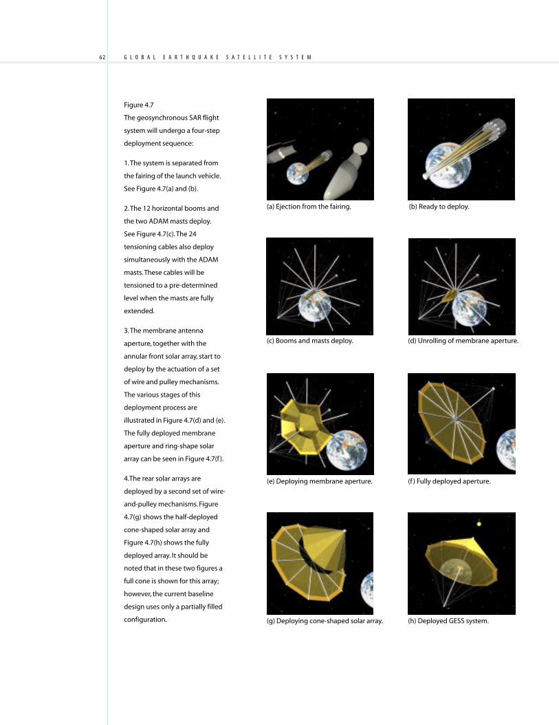
G L O B A L . E A R T H Q U A K E . S A T E L L I T E . S Y S T E M6 2

(a) Ejection from the fairing. (b) Ready to deploy.

(e) Deploying membrane aperture. (f ) Fully deployed aperture.

(g) Deploying cone-shaped solar array. (h) Deployed GESS system.

Figure 4.7

The geosynchronous SAR flight

system will undergo a four-step

deployment sequence:

1. The system is separated from

the fairing of the launch vehicle.

See Figure 4.7(a) and (b).

2. The 12 horizontal booms and

the two ADAM masts deploy.

See Figure 4.7(c). The 24

tensioning cables also deploy

simultaneously with the ADAM

masts. These cables will be

tensioned to a pre-determined

level when the masts are fully

extended.

3. The membrane antenna

aperture, together with the

annular front solar array, start to

deploy by the actuation of a set

of wire and pulley mechanisms.

The various stages of this

deployment process are

illustrated in Figure 4.7(d) and (e).

The fully deployed membrane

aperture and ring-shape solar

array can be seen in Figure 4.7(f ).

4.The rear solar arrays are

deployed by a second set of wire-

and-pulley mechanisms. Figure

4.7(g) shows the half-deployed

cone-shaped solar array and

Figure 4.7(h) shows the fully

deployed array. It should be

noted that in these two figures a

full cone is shown for this array;

however, the current baseline

design uses only a partially filled

configuration.

(c) Booms and masts deploy. (d) Unrolling of membrane aperture.

6 3GEOG E O S Y N C H R O N O U S . A R C H I T E C T U R E

would be located near the spacecraft center of

mass. Also located at the end of the nadir

mast would be a telecommunications package,

including a high-gain antenna, and an Earth

sensor for attitude control. The packages lo-

cated here would be relatively small compared

to the size of the radar antenna, so they would

not interfere with the operation of the instru-

ment. Precise knowledge of the platform po-

sition and attitude would be obtained from

the Earth sensor, Sun sensors, star trackers,

and a reverse GPS system.

Aside from the technological difficulties

posed by the instrument, several key issues

need to be addressed in the overall mission

design. Because of the great distance of

the radar from the Earth and the consequent

need for large amounts of power (up to

37 kW DC total for the spacecraft, including

28 kW for the instrument, in addition to

power for telecom, solar-electric ion propul-

sion, but not including contingency), a large

area would be required for the solar arrays.

Not only would the solar arrays constitute a

large fraction of the total spacecraft mass,

they would present a large surface area over

which solar pressure would exert forces that

perturb the spacecraft trajectory and attitude.

Several thruster fires per day would be needed

to maintain orbit control tightly enough for

high-precision repeat-pass interferometry.

It is not clear how thruster firings, whether

chemical or electric, would affect the flatness

of the radar antenna and the subsequent

system performance.

The spacecraft mass, including contin-

gency, would be around 4500 kg. In order to

maintain an adequate launch vehicle margin

of 30%, we require a launch vehicle such as

a Delta IV 4050 Heavy, as well as a Star

48 V upper stage (2455 kg). The launch

vehicle puts the spacecraft into geosynchro-

nous transfer orbit (GTO), and the Star 48 V

provides the apogee burn to produce a final

geosynchronous orbit. We further note that

more-optimal designs of several subsystems

could potentially result in mass savings of at

least several hundred kilograms.

Cost

A rough-order cost estimate for the GESS

geosynchronous SAR mission concept was

derived from Team X cost models and tech-

nology projections. With a technology cut-

off year of 2010, a 5-year development, and

15-year mission operations, the total cost for

the first satellite is in the range of $1–2 billion.

A ten-satellite constellation will cost roughly

$8–10 billion.

Future Opportunities

Seismology from Space Using Ka-BandGEO S atellite

Broadband digital seismometers — the

current state of the art in seismology — offer

continuous three-component surface dis-

placements with sensitivities in the micron

range. Although much of the world is covered

with varying densities of broadband seismom-

eters, they remain isolated to discrete point

locations.

A satellite-based, continuous measurement

of surface displacements with temporal and

spatial sensitivities appropriate for seismic

waves (submillimeter displacements, 0.01–1-Hz

sampling) would represent an important step

forward in understanding earthquake physics

and solid Earth structure and dynamics. Cur-

rent models for 3-D velocity structure of the

G L O B A L . E A R T H Q U A K E . S A T E L L I T E . S Y S T E M6 4

Earth are based on propagation of seismic

waves as measured at discrete points. Spatially

continuous mapping of seismic wave phases

from large earthquakes would allow great

improvements in crustal and lithospheric het-

erogeneity models, and would be synergistic

with current developments in super comput-

ing models of 3-D Earth structure and seis-

mic wave propagation (Figure 4.8). Detailed

images of complex wave interference would

generate significant improvements in basin

seismic resonance and earthquake hazard

assessment. By seeing the rupture unfold and

observing the amplitudes of the seismic waves

generated along the rupture, more-precise

models would be determined for the rupture

dynamics. This should lead to a fundamental

improvement in our knowledge of how earth-

quakes initiate and why they stop.

The development of a radar mission for

monitoring seismic waves involves tremen-

dous technical challenges, but it is not outside

the realm of possibility as a long-term goal.

For now, we assume that the science require-

ments for such a mission dictate a horizontal

resolution of 10 km, a vertical resolution of

100 µm, and a temporal resolution sufficient

for following 5 km/s seismic waves.

While most spaceborne imaging radars

employ aperture synthesis techniques for

obtaining high horizontal resolution, the

high-temporal resolution and wide-area cov-

erage requirement of this application preclude

the use of such techniques. That is, temporal

sampling must occur on time scales finer than

those possible for a high-altitude sensor to

traverse a synthetic aperture length. Low-

altitude sensors would be unable to provide

sufficient coverage. We consequently envision

a geostationary, real-aperture Ka-band system.

That is, in contrast to the geosynchronous

SAR, this platform must be maintained so

that it does not move relative to the Earth sur-

face. A constellation of three to five satellites

could provide coverage for all equatorial and

moderate-latitude regions of the Earth.

A short wavelength is desired so as to

maximize the interferometric sensitivity to

small surface displacements and to minimize

the required antenna area, but the frequency

must not be so great as to cause pulse-to-pulse

decorrelation through frequency drift. We

select the Ka-band frequency of 35 GHz

(8.57-mm wavelength) for this analysis as a

compromise. Therefore, in order to obtain

10-km horizontal resolution at a latitude of

±60°, an antenna with a diameter of approxi-

mately 110 m is required.

Assuming nominal system parameters,

the high antenna gain implies that the single-

pulse SNR will be greater than 40 dB for

incidence angles up to 68° with 50 kW of

radiated power and a normalized backscatter

coefficient σ0 of –20 dB. For this computa-

tion, we assume that a 1-µs gated continuous

wave (CW) pulse is transmitted. (Range reso-

lution is not required, as successive pulses are

to be interferometrically combined.) Ther-

mally induced phase noise will be much less

than the 2.2° (25 dB SNR) threshold required

for an interferometric vertical accuracy of

100 µm.

Successive pulses for each 10 km ground

cell will need to be spaced by approximately

1 s if the wave speed is 5 km/s. Given the time

between pulses, tropospheric artifacts may

pose a significant limitation on the achievable

vertical accuracy of the system (see Chapter 5,

Optimizing the Measurement). Over 1 s, the

tropospheric delay can vary by approximately

100 µm or more, depending on local condi-

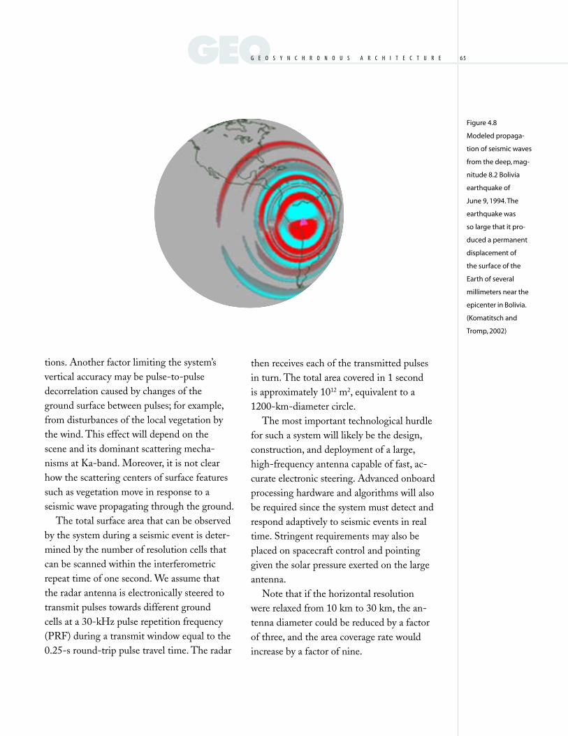
6 5GEOG E O S Y N C H R O N O U S . A R C H I T E C T U R E

Figure 4.8

Modeled propaga-

tion of seismic waves

from the deep, mag-

nitude 8.2 Bolivia

earthquake of

June 9, 1994. The

earthquake was

so large that it pro-

duced a permanent

displacement of

the surface of the

Earth of several

millimeters near the

epicenter in Bolivia.

(Komatitsch and

Tromp, 2002)

tions. Another factor limiting the system’s

vertical accuracy may be pulse-to-pulse

decorrelation caused by changes of the

ground surface between pulses; for example,

from disturbances of the local vegetation by

the wind. This effect will depend on the

scene and its dominant scattering mecha-

nisms at Ka-band. Moreover, it is not clear

how the scattering centers of surface features

such as vegetation move in response to a

seismic wave propagating through the ground.

The total surface area that can be observed

by the system during a seismic event is deter-

mined by the number of resolution cells that

can be scanned within the interferometric

repeat time of one second. We assume that

the radar antenna is electronically steered to

transmit pulses towards different ground

cells at a 30-kHz pulse repetition frequency

(PRF) during a transmit window equal to the

0.25-s round-trip pulse travel time. The radar

then receives each of the transmitted pulses

in turn. The total area covered in 1 second

is approximately 1012 m2, equivalent to a

1200-km-diameter circle.

The most important technological hurdle

for such a system will likely be the design,

construction, and deployment of a large,

high-frequency antenna capable of fast, ac-

curate electronic steering. Advanced onboard

processing hardware and algorithms will also

be required since the system must detect and

respond adaptively to seismic events in real

time. Stringent requirements may also be

placed on spacecraft control and pointing

given the solar pressure exerted on the large

antenna.

Note that if the horizontal resolution

were relaxed from 10 km to 30 km, the an-

tenna diameter could be reduced by a factor

of three, and the area coverage rate would

increase by a factor of nine.

G L O B A L . E A R T H Q U A K E . S A T E L L I T E . S Y S T E M6 6

C H A P T E R

F I V E

easuring surface deformation from space at

the required accuracy and frequency for earthquake

studies constitutes numerous challenges. Methods to

improve the measurement capabilities presented in

this report include the possibility of using a medium

Earth orbit (MEO), and developing ways to reduce the

noise from atmospheric effects.

M

Optimizing the Measurement

Inset: Simulated tropospheric delay. Background: Orbit path and footprint from a

MEO spacecraft for GESS.

6 7

Spectrum of Options: LEO+, MEO, GEO

The mission concepts explored in this study

constitute the extremes of a range of options

for a global earthquake-monitoring satellite

system. The LEO and LEO+ concepts, which

have many similarities, are near-term possi-

bilities that entail the use of conventional tech-

nology in mission architectures akin to those

of existing SAR spacecraft. On the other hand,

the geosynchronous concept is an ambitious,

far-term possibility that would be dramatically

different from any current SAR system in terms

of its technology, operation, and performance.

A middle ground may be possible, and in fact

potentially desirable.

The main differences between the LEO/

LEO+ concepts and the geosynchronous con-

cept arise from the disparity in the satellite

orbital altitudes — around 1000 km for the

LEO/LEO+ cases vs. 35,800 km for the geo-

synchronous case. Higher-altitude orbits place

more demanding requirements on the radar

instrument: Considerably more power is

required, as well as a physically larger radar

antenna in order to maintain acceptable

range-Doppler ambiguity performance. At

the same time, higher orbits also provide

more comprehensive Earth coverage as well.

Although a sensor’s area coverage rate for

fixed resolution is limited by range-Doppler

ambiguities and is consequently independent

of altitude, a higher-altitude sensor would

generally have land areas of interest in view

more often, so the effective or “useful” cover-

age rate would be greater for higher-altitude

sensors. A SAR constellation at MEO (be-

tween around the LEO and GEO altitudes)

might strike a good balance between instru-

ment complexity and Earth coverage.

Under the assumption that the SAR

visible-swath width is limited by the ground-

incidence angle, the visible-swath width in-

creases with altitude, as depicted in Figure 5.1.

Points are marked on these curves at altitudes

Figure 5.1

Plots of one-sided

SAR swath width for

different ground

incidence angle

limits as a function

of platform altitude.

Markers are for LEO,

LEO+, and GEO

satellites.

OPTIMIZATIONO P T I M I Z I N G . T H E . M E A S U R E M E N T

9000

8000

7000

6000

5000

4000

3000

2000

1000

0.5 1 1.5 2 2.5 3 3.5 4 4.50

Wid

th o

f Vis

ible

Sw

ath

(km

)

Orbit Altitude (km) × 104

10–80° Ground Incidence25–65° Ground Incidence

G L O B A L . E A R T H Q U A K E . S A T E L L I T E . S Y S T E M6 8

corresponding to the LEO (800 km), LEO+

(1325 km), and geosynchronous (35,800 km)

concepts. As the altitude increases towards

infinity, the visible-swath width approaches

an asymptotic limit determined by the curva-

ture of the Earth. An incremental change in

orbit altitude thus has a much greater impact

on the swath width at lower altitudes than at

higher ones.

Considering broadside image acquisitions

only, a crude estimate of a SAR platform’s

two-sided daily coverage area might be com-

puted by multiplying the two-sided visible

swath widths of Figure 5.1 by the average

nadir velocity of the spacecraft and integrat-

ing over one day. Plots of such estimates are

shown in Figure 5.2. (Note that ground areas

can come into view several times per day, so

the coverage area plotted can be larger than

the total surface area of the Earth.) Because

the nadir velocity decreases with altitude

while the swath width increases, these curves

peak at MEO altitudes. Such estimates of the

daily coverage area are somewhat oversimpli-

fied, however. These estimates do not account

for areas accessible through squinted acquisi-

tion geometries (see Figure 5.3), and the finite

along-track footprint widths of high-altitude

sensors can have a dramatic effect on Earth

coverage. The estimates also do not account

for the ground-track curvature typical of high-

altitude orbits, nor do they account for the fact

that high-altitude orbits might be more easily

designed for better coverage of particular tar-

get areas. Furthermore, it may be more diffi-

cult to obtain two-sided coverage from lower

altitudes since doing so would likely require

mechanical rather than electronic antenna

beam steering. These factors imply that, in

practice, the effective peaks in daily coverage

might occur at MEO altitudes somewhat

higher than shown in Figure 5.2. More de-

tailed system trade analyses and cost studies

Figure 5.2

Two-sided daily

broadside coverage

area as a function

of platform altitude

assuming broad-

side acquisitions

only. The locations

of the peaks will

be at higher MEO

altitudes if other

factors are

considered. Markers

are for LEO, LEO+,

and GEO satellites.

3.5

3

2.5

2

1.5

1

0.5

0.5 1 1.5 2 2.5 3 3.5 4 4.5

2 (S

wat

h W

idth

) (A

vera

ge

Gro

un

d V

elo

city

) (1

Day

) (km

2 )

Orbit Altitude (km)

10–80° Ground Incidence25–65° Ground Incidence

0

× 109

× 104

6 9

would be required to determine the optimal

satellite altitude given the factors described

above.

Figure 5.3 is perhaps more telling of the

Earth-coverage advantages of high-altitude

sensors. This plot shows the two-sided in-

stantaneously accessible area, or in other

words, the area of the two-sided sensor visible

footprint. For low to moderate orbital alti-

tudes (i.e., before the break point at about

18,000 km altitude), the along-track width

of the sensor footprint is limited by the maxi-

mum azimuth angle to which the radar an-

tenna beam can be steered electronically. At

higher altitudes, the along-track footprint

width is limited by the squint angle on the

ground. The curves shown assume up to

±15° of azimuth beam steering and up to

±60° of ground squint. For the case of the

lower curve, the footprint of the geosynchro-

nous sensor is approximately 30 times larger

than that of the LEO+ sensor. On the other

hand, a MEO sensor at half the altitude of

the geosynchronous sensor (17,900 km)

would have a footprint area 83% of the size

of its geosynchronous counterpart.

Clearly, the goal of around-the-clock ac-

cessibility for quick-response imaging favors

the use of higher-altitude sensors. As the sat-

ellite relative velocity decreases with altitude,

however, the integration time required to

form an image may become significant com-

pared to the event-response time. The average

integration time required for 10-m resolution

is shown in Figure 5.4. For the geosynchro-

nous case, the integration time could be up to

several minutes. This factor would need to be

accounted for in more detailed trade studies.

High-altitude SAR systems could provide

extensive Earth coverage, but their associated

demands on the radar hardware cannot be ne-

glected. Figure 5.5 illustrates the relationship

Figure 5.3

Two-sided

instantaneous

accessibility. Area of

the sensor two-sided

visible footprint as a

function of platform

altitude. Markers are

for LEO, LEO+, and

GEO satellites.

OPTIMIZATIONO P T I M I Z I N G . T H E . M E A S U R E M E N T

12

10

8

6

4

2

00.5 1 1.5 2 2.5 3 3.5 4 4.5

Inst

anta

neo

usl

y V

isib

le G

rou

nd

Are

a (k

m2 )

Orbit Altitude (km)

× 107

× 104

10–80° Ground Incidence25–65° Ground Incidence

G L O B A L . E A R T H Q U A K E . S A T E L L I T E . S Y S T E M7 0

Figure 5.4

Synthetic aperture

integration time

required for

10-m resolution

as a function of

platform altitude.

The required

integration time

can be several

minutes or more

at high altitudes.

Markers are for

LEO, LEO+, and

GEO satellites.

5

4.5

4

3.5

3

2.5

2

1.5

1

0.5

0

Ave

rag

e In

teg

rati

on

Tim

e (m

in)

0.5 1 1.5 2 2.5 3 3.5 4 4.5

× 104Orbit Altitude (km)

80° Ground Incidence10° Ground Incidence

Figure 5.5

Ideal minimum

antenna area as

a function of

platform altitude

for various max-

imum ground

incidence angles.

Higher platform

altitudes require

larger antenna

apertures. Markers

are for LEO, LEO+,

and GEO satellites.

4000

3500

3000

2500

2000

1500

1000

500

0

Min

imu

m A

nte

nn

a A

rea

(m2 )

80° Ground Incidence65° Ground Incidence50° Ground Incidence

Orbit Altitude (km)

0.5 1 1.5 2 2.5 3 3.5 4 4.5

× 104

7 1

between the orbital altitude and the required

ideal antenna area for a number of different

ground incidence angles. The required an-

tenna area is driven by the need to avoid

range-Doppler ambiguities and increases with

both altitude and ground incidence angle.

Higher altitudes place less-severe require-

ments on the electronic-steering capabilities

of the radar antenna, however. Figure 5.6

depicts, as functions of altitude, the far-range

look angles corresponding to two different

far-range ground incidence angles. For nadir-

pointed antennas, the far-range look angle

is equal to the maximum elevation steering

angle. From the curves shown, it is evident

that electronic beam steering from side to side

would be quite challenging at lower altitudes.

Although the parametric analyses pre-

sented in this section are somewhat simplified,

they strongly suggest that MEO architectures

deserve further consideration. A constellation

of SAR sensors in MEO orbits could likely

provide performance similar to that expected

from a geosynchronous constellation while

doing so with smaller antennas, reduced

power, and lower launch costs. Space radiation

at MEO altitudes is known to be rather severe,

but because the specific characteristics of the

radiation environment (e.g., particle energies)

must also be considered in the context of the

eventual system design, MEO orbits might

still be ideal for future SAR missions.

Atmospheric Analysis and Mitigation

Another method for improving measure-

ments from a GESS is to mitigate atmospheric

noise effects. Because InSAR observations of

surface displacement are obtained through the

measurement of signal time delays, variability

in the signal propagation properties of the at-

mosphere can seriously degrade the accuracy

of the InSAR technique. If not accounted for,

minute changes in the atmosphere’s index of

refraction can lead to data artifacts that are

Figure 5.6

Far-range look

angle as a function

of platform

altitude. Because

of the greater

variation in look

angle, side-to-side

electronic beam

steering is more

difficult from lower

altitudes. Markers

are for LEO, LEO+,

and GEO satellites.

OPTIMIZATIONO P T I M I Z I N G . T H E . M E A S U R E M E N T

80° Ground Incidence65° Ground Incidence

Far

Ran

ge

Loo

k A

ng

le (d

eg)

80

70

60

50

40

30

20

10

00.5 1 1.5 2 2.5 3 3.5 4 4.5

× 104Orbit Altitude (km)

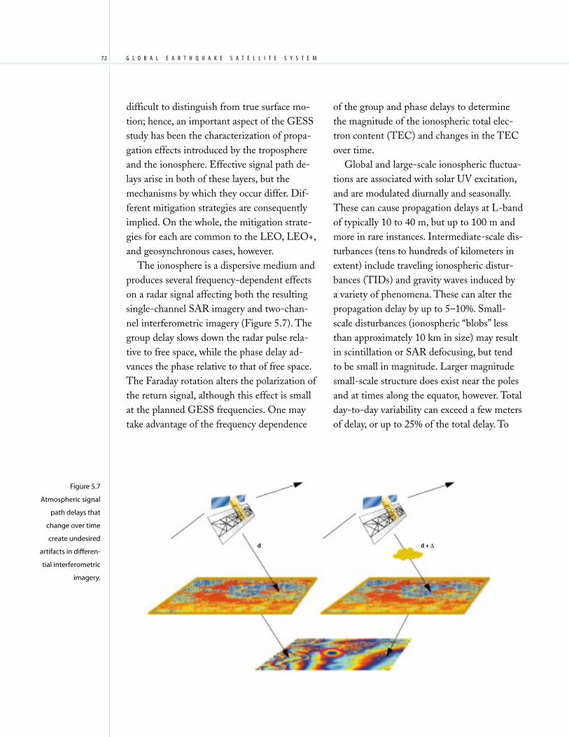
G L O B A L . E A R T H Q U A K E . S A T E L L I T E . S Y S T E M7 2

difficult to distinguish from true surface mo-

tion; hence, an important aspect of the GESS

study has been the characterization of propa-

gation effects introduced by the troposphere

and the ionosphere. Effective signal path de-

lays arise in both of these layers, but the

mechanisms by which they occur differ. Dif-

ferent mitigation strategies are consequently

implied. On the whole, the mitigation strate-

gies for each are common to the LEO, LEO+,

and geosynchronous cases, however.

The ionosphere is a dispersive medium and

produces several frequency-dependent effects

on a radar signal affecting both the resulting

single-channel SAR imagery and two-chan-

nel interferometric imagery (Figure 5.7). The

group delay slows down the radar pulse rela-

tive to free space, while the phase delay ad-

vances the phase relative to that of free space.

The Faraday rotation alters the polarization of

the return signal, although this effect is small

at the planned GESS frequencies. One may

take advantage of the frequency dependence

of the group and phase delays to determine

the magnitude of the ionospheric total elec-

tron content (TEC) and changes in the TEC

over time.

Global and large-scale ionospheric fluctua-

tions are associated with solar UV excitation,

and are modulated diurnally and seasonally.

These can cause propagation delays at L-band

of typically 10 to 40 m, but up to 100 m and

more in rare instances. Intermediate-scale dis-

turbances (tens to hundreds of kilometers in

extent) include traveling ionospheric distur-

bances (TIDs) and gravity waves induced by

a variety of phenomena. These can alter the

propagation delay by up to 5–10%. Small-

scale disturbances (ionospheric “blobs” less

than approximately 10 km in size) may result

in scintillation or SAR defocusing, but tend

to be small in magnitude. Larger magnitude

small-scale structure does exist near the poles

and at times along the equator, however. Total

day-to-day variability can exceed a few meters

of delay, or up to 25% of the total delay. To

Figure 5.7

Atmospheric signal

path delays that

change over time

create undesired

artifacts in differen-

tial interferometric

imagery.

d d + ∆

7 3OPTIMIZATIONO P T I M I Z I N G . T H E . M E A S U R E M E N T

Figure 5.8

Due to the

ionosphere, the

range of objects

in the image

changes with

frequency.

SAR

Ionosphere

Frequency-1

Frequency-2

Averaged range difference

measured to < 1 m determines

ionosphere to < 30 TECU

observe range changes at the centimeter level,

the ionospheric effects must be removed

almost completely.

We have examined two dual-frequency, or

split-spectrum, scenarios. In the first, we as-

sume that GESS transmits a chirp waveform

at two L-band (~1250 MHz) frequencies,

each 10 MHz wide, separated by 70 MHz.

In the second, we envision an additional

C-band antenna transmitting a 10 MHz-wide

chirp centered at 5350 MHz. We have ap-

plied concepts to interferometric SAR similar

to those developed for removing ionospheric

effects from GPS signals using the GPS

dual frequency range and phase observables.

Although there are significant differences

between GPS and SAR, much work appears

applicable. These dual-frequency approaches

appear to be capable of removing the iono-

sphere at the level that GESS requires, at

least for intermediate- and larger-scale

ionospheric features (10 km and up).

Splitting the spectrum for a single epoch, a

single pass of SAR data permits an estimate

of the total ionospheric range delay measure-

ment. The apparent range difference of iden-

tical features in the split-spectrum images is

where the range offset is proportional to T,

the line-of-site TEC of the ionosphere, and

to the difference of the squared inverses of the

two frequencies (Figure 5.8). The larger the

frequency difference, the larger the effect,

although for very different frequencies, the

ground imagery changes significantly in other

ways. By averaging the observed range offset

over areas about 20 km across (depending

on terrain and ground features), the total

ionospheric delay may be determined to as

little as 0.5 TEC units (TECU), equivalent to

about 10 cm of ground displacement for dif-

ferential interferometry.

Splitting the spectrum for two-epoch dif-

ferential interferometry yields a higher preci-

sion estimate of the change in the ionosphere

between the two epochs, but no information

about the total ionospheric delay. The change

in scaled phase due to ionospheric effects is

where the phase difference is proportional to

the change in state of the ionosphere, ∆T. By

averaging the interferometric range difference

over large enough areas (~10 km on a side),

the change in the ionosphere at the required

level (0.05 TEC units is approximately 1 cm)

may be determined. Thus, intermediate-sized

ionospheric perturbations can be estimated

and removed from the interferometric data

(Figure 5.9). Large-amplitude, smaller-scale

perturbations may prove extremely difficult to

remove, however.

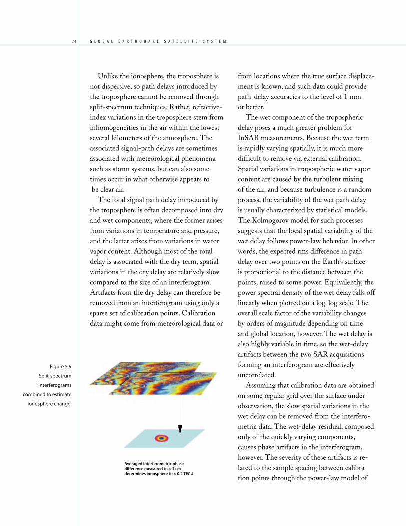
G L O B A L . E A R T H Q U A K E . S A T E L L I T E . S Y S T E M7 4

Unlike the ionosphere, the troposphere is

not dispersive, so path delays introduced by

the troposphere cannot be removed through

split-spectrum techniques. Rather, refractive-

index variations in the troposphere stem from

inhomogeneities in the air within the lowest

several kilometers of the atmosphere. The

associated signal-path delays are sometimes

associated with meteorological phenomena

such as storm systems, but can also some-

times occur in what otherwise appears to

be clear air.

The total signal path delay introduced by

the troposphere is often decomposed into dry

and wet components, where the former arises

from variations in temperature and pressure,

and the latter arises from variations in water

vapor content. Although most of the total

delay is associated with the dry term, spatial

variations in the dry delay are relatively slow

compared to the size of an interferogram.

Artifacts from the dry delay can therefore be

removed from an interferogram using only a

sparse set of calibration points. Calibration

data might come from meteorological data or

from locations where the true surface displace-

ment is known, and such data could provide

path-delay accuracies to the level of 1 mm

or better.

The wet component of the tropospheric

delay poses a much greater problem for

InSAR measurements. Because the wet term

is rapidly varying spatially, it is much more

difficult to remove via external calibration.

Spatial variations in tropospheric water vapor

content are caused by the turbulent mixing

of the air, and because turbulence is a random

process, the variability of the wet path delay

is usually characterized by statistical models.

The Kolmogorov model for such processes

suggests that the local spatial variability of the

wet delay follows power-law behavior. In other

words, the expected rms difference in path

delay over two points on the Earth’s surface

is proportional to the distance between the

points, raised to some power. Equivalently, the

power spectral density of the wet delay falls off

linearly when plotted on a log-log scale. The

overall scale factor of the variability changes

by orders of magnitude depending on time

and global location, however. The wet delay is

also highly variable in time, so the wet-delay

artifacts between the two SAR acquisitions

forming an interferogram are effectively

uncorrelated.

Assuming that calibration data are obtained

on some regular grid over the surface under

observation, the slow spatial variations in the

wet delay can be removed from the interfero-

metric data. The wet-delay residual, composed

only of the quickly varying components,

causes phase artifacts in the interferogram,

however. The severity of these artifacts is re-

lated to the sample spacing between calibra-

tion points through the power-law model of

Figure 5.9

Split-spectrum

interferograms

combined to estimate

ionosphere change.

Averaged interferometric phasedifference measured to < 1 cmdetermines ionosphere to < 0.4 TECU

7 5

the turbulence process, with artifacts becom-

ing less severe as the grid of calibration points

is made finer. Calibration data might com-

prise water-vapor estimates obtained from

GPS or water vapor radiometer (WVR)

instruments on the ground as well as down-

ward-looking instruments on board the

spacecraft. If calibration data are acquired

every 10 to 100 km, the residual wet delay

can be reduced to the level of 1 cm (see Fig-

ure 5.10). Calibration grids much finer than

this may be impractical. Mesoscale atmo-

spheric data assimilation models may provide

data at fine resolution to correct the delay.

The residual variability in the wet delay

can be further reduced through the averaging

or “stacking” of multiple interferometric data

OPTIMIZATIONO P T I M I Z I N G . T H E . M E A S U R E M E N T

sets (Sandwell and Fialko, 2002; Webb et al.,

2002). Stacking reduces artifacts and noise

from other sources as well, though data limi-

tations and the desire to preserve temporal

resolution imply that artifacts cannot be

eliminated entirely. Advances in data-pro-

cessing techniques may also offer ways of

removing some tropospheric artifacts. Never-

theless, relative to other sources of error, the

wet component of the tropospheric delay

may prove to be a limiting factor in the accu-

racy of the interferometric technique if the

goal is to observe millimeter-scale surface

displacements. More research on this topic

is required to support subcentimeter-scale

displacement accuracies.

Figure 5.10

Residual one-way

differential tropo-

spheric zenith

display comparing

theoretical models

and several data

sets as calibration.

The modeled

residual wet tropo-

spheric delay

decreases with

increased sampling

rate.

Spatial Sampling Rate (1/km)

20

15

10

5

010–2 10–1 100 101

PiecewisePower-LawModel

RM

S D

iffe

ren

tial

Del

ay (m

m)

Williamset al., 1998:GPS (SouthernCalifornia)

Hanssen,2001: InSAR(Groningen, TheNetherlands)

Zebker et al.,1997: InSAR(Big Island, Hawaii)

Treuhaft and Lanyi,1987: Theory+WVR(Goldstone, California)

Goldstein,1995: InSAR+WVR(Mojave Desert, California)

G L O B A L . E A R T H Q U A K E . S A T E L L I T E . S Y S T E M7 6

Technology Studies

C H A P T E R

S I X

GESS has studied SAR constellations from low-earth to geosynchronous orbits.

These SAR missions place a significant demand on the spacecraft resources (mass,

power, data rate). Revolutionary antenna technologies are required to enable the

GEO and MEO systems described. High-efficiency integrated (single-chip) T/R

modules are necessary to ensure the mass, power, and cost of the modules are not

prohibitively high when thousands of modules are required. Adaptive scanning

and phase self-compensation techniques will be necessary to alleviate require-

ments on antenna flatness. Modular or distributed architectures will enable these

systems to be very flexible. Radiation-tolerant electronics are also a major chal-

lenge, particularly for the antenna electronics, which have only limited shielding.

For the GESS study, three technology studies were completed to address the need

for large deployable electronically steered antennas and for a general reduction of

radar instrument mass and power. By ultimately reducing the instrument cost, SAR

constellations could be enabled. The three tasks were:

• Low-Power Chirp Generator: Demonstrate a miniaturized, low-power, rad-hard

chirp generator, which is modular and flexible such that the design is directly

applicable to GESS as well as other high-performance radar missions.

• High-Efficiency Transmitter Module: Demonstrate an ultrahigh-efficiency L-band

Class-E/F amplifier for use in phased-array transmit/receive modules.

• Geosynchronous SAR Antenna: Conduct design and technology trades to

establish the geosynchronous SAR antenna architecture to assess overall mission

feasibility and identify the technology roadmap.

7 7

Low-Power Chirp Generator

The goal of this activity was to reduce the

power consumption of the chirp generator by

a factor of five from similar SIR-C/SRTM

hardware. In this task, we have demonstrated

a low-power, high-bandwidth, reconfigurable

digital chirp generator (DCG) for use as a

basic building block scalable to a variety of

system applications.

Many NASA radar systems operate at

L-band or include an L-band intermediate

frequency as part of a higher-frequency sys-

tem. Linear FM chirp waveforms are used for

pulse compression. For signal repeatability

and flexibility, DCG technology was chosen.

The DCG must be frequency agile with the

ability to switch between frequencies in a

few nanoseconds. The DCG should produce

spectrally pure signals (high spurious free

dynamic range) and capable of 80-MHz chirp

bandwidth.

Minimizing the DC power consumption

was a major design goal. When distributed

signal generation is required, such as in radar

systems implementing an active array antenna

requiring hundreds or even thousands of indi-

vidual DCGs, then power considerations are

paramount.

A final major design goal was to ensure

that the DCG would endure the space envi-

ronment. A combination of radiation testing

and consultations with radiation testing ex-

perts was performed to address this issue.

Te c h n i c a l C h a l l e n g e s

Two candidate technologies were evalu-

ated. The first was based on gallium arsenide

(GaAs) technology (STEL-2375A) and the

second was based on silicon CMOS technol-

ogy (AD9854). The differing fabrication pro-

cess of these two devices leads directly to

almost all of their respective strengths and

weaknesses. High-frequency and high-band-

width digital synthesizers must run at very

high frequencies to satisfy the Nyquist limit.

High-frequency digital systems invariably

require more power than those of lower oper-

ating frequencies do. GaAs can run at speeds

considerably higher than CMOS, but also

consumes more power. Also, the power re-

quirements for GaAs are practically indepen-

dent of its operating speed. Therefore, one

cannot choose to reduce power simply by re-

ducing the speed. In contrast, CMOS requires

less power to operate, and its power consump-

tion is directly related to its operating speed,

although it cannot run at the maximum

speeds of GaAs. If a particular radar system

requires less bandwidth, the AD9854 device

may be run at slower speeds. In comparison,

the STEL-2375A requires 15 W regardless

of clocking speed or output frequency.

The AD9854 is hampered by its lower

maximum frequency output of 120 MHz.

While 120 MHz easily covers the required

80-MHz bandwidth, the signal must be

“mixed up” to L-band through heterodyning.

A fundamental problem with upconverting

low-frequency signals is the close-in image

frequency. Unless a multiple-stage upconver-

sion approach is adopted, the image filter is

often difficult to realize. The AD9854 is able

to overcome this disadvantage by having In-

phase and Quadrature (IQ) outputs. These

signals can be fed into an IQ mixer to cancel

the undesired side band. One technical chal-

lenge is created when using IQ modulation.

The IQ outputs must be matched to a quadra-

ture mixer that can handle DC-120-MHz

input and L-band output. A survey of avail-

able components revealed this to be a non-

trivial challenge.

TECHNOLOGYT E C H N O L O G Y . S T U D I E S

G L O B A L . E A R T H Q U A K E . S A T E L L I T E . S Y S T E M7 8

A major challenge for the AD9854 is its ra-

diation susceptibility. While the STEL-2375A

is inherently rad-hard, the reliable operation

of the AD9854 in a high-radiation environ-

ment is of concern. This is because it is a

silicon (rather than GaAs) device using a

commercial (non-rad-hard) fabrication

process.

E n a b l i n g Te c h n o l o g i e s

Two semiconductor technologies were

evaluated for use as the core-component

of a low-power, rad-hard DCG. The first

DCG-core is the ITT Microwave (formerly

Stanford Telecom) STEL-2375A, which is

a hybrid microcircuit composed of a GaAs

numerically controlled oscillator (NCO) and

a CMOS DAC. The NCO performs all of the

basic functions of the DCG and the DAC

converts the digital signal to an analog wave-

form. The NCO runs up to 1 GHz, which

means it can faithfully produce an analog sig-

nal up to 400 MHz. The second DCG-core

is the Analog Devices AD9854, which is a

0.35-µm CMOS device. This device runs up

to 300 MHz, which means it can faithfully

produce an analog signal up to 120 MHz.

The STEL-2375A uses advanced high-

speed digital GaAs technology. This tech-

nology is newer than silicon technologies,

such as CMOS, but mature enough to have

an established record. GaAs is well suited for

space-based missions as it is naturally radia-

tion tolerant, and its reliability has tested well.

Newer materials, such as silicon germanium

(SiGe), may become a more practical alterna-

tive as speeds increase. However, the radiation

susceptibility of SiGe is currently unknown.

The AD9854 device is not new, but its new

0.35-µm CMOS fabrication process allows

for high speeds and unique capabilities.

Recent advances in well-balanced, high-fre-

quency SiGe quadrature mixers have enabled

us to take advantage of the quadrature outputs

of the AD9854.

R e s u l t s

The STEL-2375A and the AD9854 were

each prototyped using an FPGA as an inter-

face and controller. The DCG based on the

STEL-2375A is shown in Figure 6.1(a) and

the DCG based on the AD9854 is shown

in Figure 6.1(b). Testing of these devices in-

cluded DC power consumption over all oper-

ating modes, spurious free dynamic range,

and features testing (i.e., chirp, CW, standby

modes). Radiation testing was also performed

on the AD9854.

Figure 6.1

Digital chirp

generators.

(a) STEL-2375A digital chirp generator.

(b) AD9854 digital chirp generator.

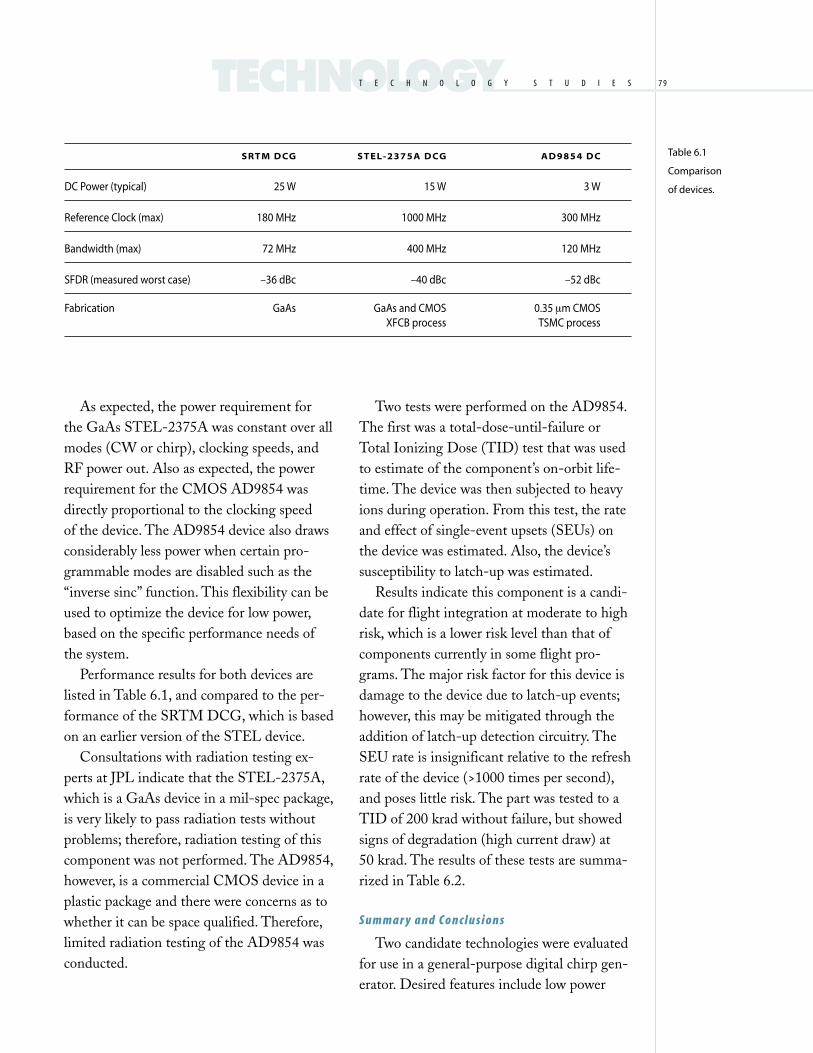
7 9

As expected, the power requirement for

the GaAs STEL-2375A was constant over all

modes (CW or chirp), clocking speeds, and

RF power out. Also as expected, the power

requirement for the CMOS AD9854 was

directly proportional to the clocking speed

of the device. The AD9854 device also draws

considerably less power when certain pro-

grammable modes are disabled such as the

“inverse sinc” function. This flexibility can be

used to optimize the device for low power,

based on the specific performance needs of

the system.

Performance results for both devices are

listed in Table 6.1, and compared to the per-

formance of the SRTM DCG, which is based

on an earlier version of the STEL device.

Consultations with radiation testing ex-

perts at JPL indicate that the STEL-2375A,

which is a GaAs device in a mil-spec package,

is very likely to pass radiation tests without

problems; therefore, radiation testing of this

component was not performed. The AD9854,

however, is a commercial CMOS device in a

plastic package and there were concerns as to

whether it can be space qualified. Therefore,

limited radiation testing of the AD9854 was

conducted.

Two tests were performed on the AD9854.

The first was a total-dose-until-failure or

Total Ionizing Dose (TID) test that was used

to estimate of the component’s on-orbit life-

time. The device was then subjected to heavy

ions during operation. From this test, the rate

and effect of single-event upsets (SEUs) on

the device was estimated. Also, the device’s

susceptibility to latch-up was estimated.

Results indicate this component is a candi-

date for flight integration at moderate to high

risk, which is a lower risk level than that of

components currently in some flight pro-

grams. The major risk factor for this device is

damage to the device due to latch-up events;

however, this may be mitigated through the

addition of latch-up detection circuitry. The

SEU rate is insignificant relative to the refresh

rate of the device (>1000 times per second),

and poses little risk. The part was tested to a

TID of 200 krad without failure, but showed

signs of degradation (high current draw) at

50 krad. The results of these tests are summa-

rized in Table 6.2.

S u m m a r y a n d C o n c l u s i o n s

Two candidate technologies were evaluated

for use in a general-purpose digital chirp gen-

erator. Desired features include low power

Table 6.1

Comparison

of devices.

TECHNOLOGYT E C H N O L O G Y . S T U D I E S

S RT M D CG ST E L - 2 3 7 5 A D CG A D 9 8 5 4 D C

DC Power (typical) 25 W 15 W 3 W

Reference Clock (max) 180 MHz 1000 MHz 300 MHz

Bandwidth (max) 72 MHz 400 MHz 120 MHz

SFDR (measured worst case) –36 dBc –40 dBc –52 dBc

Fabrication GaAs GaAs and CMOS 0.35 µm CMOSXFCB process TSMC process

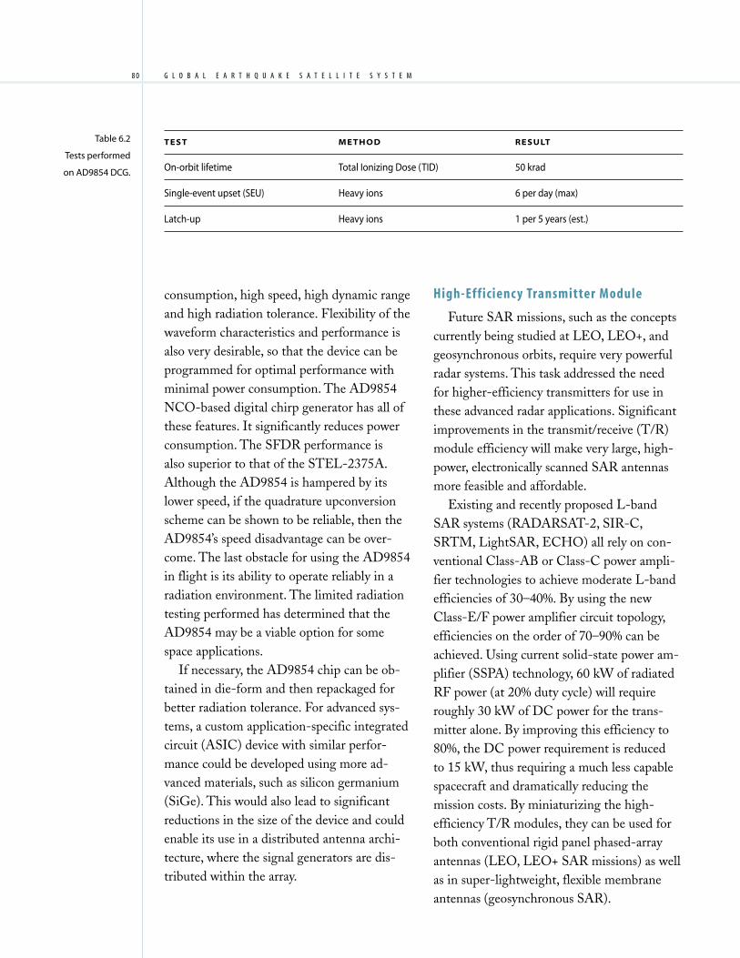
G L O B A L . E A R T H Q U A K E . S A T E L L I T E . S Y S T E M8 0

consumption, high speed, high dynamic range

and high radiation tolerance. Flexibility of the

waveform characteristics and performance is

also very desirable, so that the device can be

programmed for optimal performance with

minimal power consumption. The AD9854

NCO-based digital chirp generator has all of

these features. It significantly reduces power

consumption. The SFDR performance is

also superior to that of the STEL-2375A.

Although the AD9854 is hampered by its

lower speed, if the quadrature upconversion

scheme can be shown to be reliable, then the

AD9854’s speed disadvantage can be over-

come. The last obstacle for using the AD9854

in flight is its ability to operate reliably in a

radiation environment. The limited radiation

testing performed has determined that the

AD9854 may be a viable option for some

space applications.

If necessary, the AD9854 chip can be ob-

tained in die-form and then repackaged for

better radiation tolerance. For advanced sys-

tems, a custom application-specific integrated

circuit (ASIC) device with similar perfor-

mance could be developed using more ad-

vanced materials, such as silicon germanium

(SiGe). This would also lead to significant

reductions in the size of the device and could

enable its use in a distributed antenna archi-

tecture, where the signal generators are dis-

tributed within the array.

Table 6.2

Tests performed

on AD9854 DCG.

High-Efficienc y Transmitter Module

Future SAR missions, such as the concepts

currently being studied at LEO, LEO+, and

geosynchronous orbits, require very powerful

radar systems. This task addressed the need

for higher-efficiency transmitters for use in

these advanced radar applications. Significant

improvements in the transmit/receive (T/R)

module efficiency will make very large, high-

power, electronically scanned SAR antennas

more feasible and affordable.

Existing and recently proposed L-band

SAR systems (RADARSAT-2, SIR-C,

SRTM, LightSAR, ECHO) all rely on con-

ventional Class-AB or Class-C power ampli-

fier technologies to achieve moderate L-band

efficiencies of 30–40%. By using the new

Class-E/F power amplifier circuit topology,

efficiencies on the order of 70–90% can be

achieved. Using current solid-state power am-

plifier (SSPA) technology, 60 kW of radiated

RF power (at 20% duty cycle) will require

roughly 30 kW of DC power for the trans-

mitter alone. By improving this efficiency to

80%, the DC power requirement is reduced

to 15 kW, thus requiring a much less capable

spacecraft and dramatically reducing the

mission costs. By miniaturizing the high-

efficiency T/R modules, they can be used for

both conventional rigid panel phased-array

antennas (LEO, LEO+ SAR missions) as well

as in super-lightweight, flexible membrane

antennas (geosynchronous SAR).

T E S T M E T H O D R E S U LT

On-orbit lifetime Total Ionizing Dose (TID) 50 krad

Single-event upset (SEU) Heavy ions 6 per day (max)

Latch-up Heavy ions 1 per 5 years (est.)

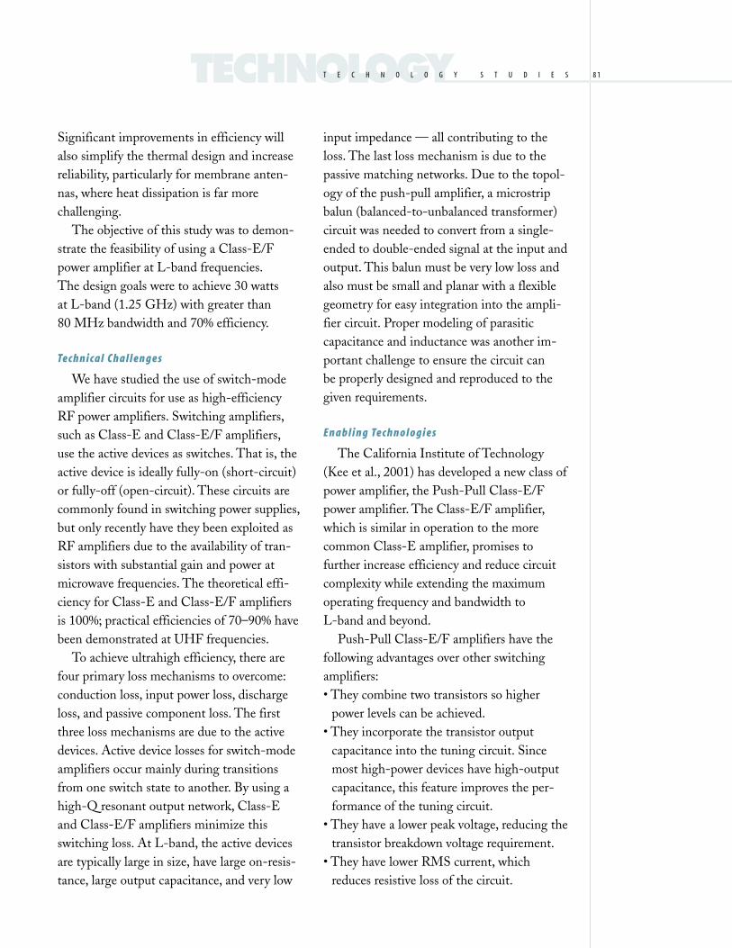
8 1

Significant improvements in efficiency will

also simplify the thermal design and increase

reliability, particularly for membrane anten-

nas, where heat dissipation is far more

challenging.

The objective of this study was to demon-

strate the feasibility of using a Class-E/F

power amplifier at L-band frequencies.

The design goals were to achieve 30 watts

at L-band (1.25 GHz) with greater than

80 MHz bandwidth and 70% efficiency.

Te c h n i c a l C h a l l e n g e s

We have studied the use of switch-mode

amplifier circuits for use as high-efficiency

RF power amplifiers. Switching amplifiers,

such as Class-E and Class-E/F amplifiers,

use the active devices as switches. That is, the

active device is ideally fully-on (short-circuit)

or fully-off (open-circuit). These circuits are

commonly found in switching power supplies,

but only recently have they been exploited as

RF amplifiers due to the availability of tran-

sistors with substantial gain and power at

microwave frequencies. The theoretical effi-

ciency for Class-E and Class-E/F amplifiers

is 100%; practical efficiencies of 70–90% have

been demonstrated at UHF frequencies.

To achieve ultrahigh efficiency, there are

four primary loss mechanisms to overcome:

conduction loss, input power loss, discharge

loss, and passive component loss. The first

three loss mechanisms are due to the active

devices. Active device losses for switch-mode

amplifiers occur mainly during transitions

from one switch state to another. By using a

high-Q resonant output network, Class-E

and Class-E/F amplifiers minimize this

switching loss. At L-band, the active devices

are typically large in size, have large on-resis-

tance, large output capacitance, and very low

input impedance — all contributing to the

loss. The last loss mechanism is due to the

passive matching networks. Due to the topol-

ogy of the push-pull amplifier, a microstrip

balun (balanced-to-unbalanced transformer)

circuit was needed to convert from a single-

ended to double-ended signal at the input and

output. This balun must be very low loss and

also must be small and planar with a flexible

geometry for easy integration into the ampli-

fier circuit. Proper modeling of parasitic

capacitance and inductance was another im-

portant challenge to ensure the circuit can

be properly designed and reproduced to the

given requirements.

E n a b l i n g Te c h n o l o g i e s

The California Institute of Technology

(Kee et al., 2001) has developed a new class of

power amplifier, the Push-Pull Class-E/F

power amplifier. The Class-E/F amplifier,

which is similar in operation to the more

common Class-E amplifier, promises to

further increase efficiency and reduce circuit

complexity while extending the maximum

operating frequency and bandwidth to

L-band and beyond.

Push-Pull Class-E/F amplifiers have the

following advantages over other switching

amplifiers:

• They combine two transistors so higher

power levels can be achieved.

• They incorporate the transistor output

capacitance into the tuning circuit. Since

most high-power devices have high-output

capacitance, this feature improves the per-

formance of the tuning circuit.

• They have a lower peak voltage, reducing the

transistor breakdown voltage requirement.

• They have lower RMS current, which

reduces resistive loss of the circuit.

TECHNOLOGYT E C H N O L O G Y . S T U D I E S

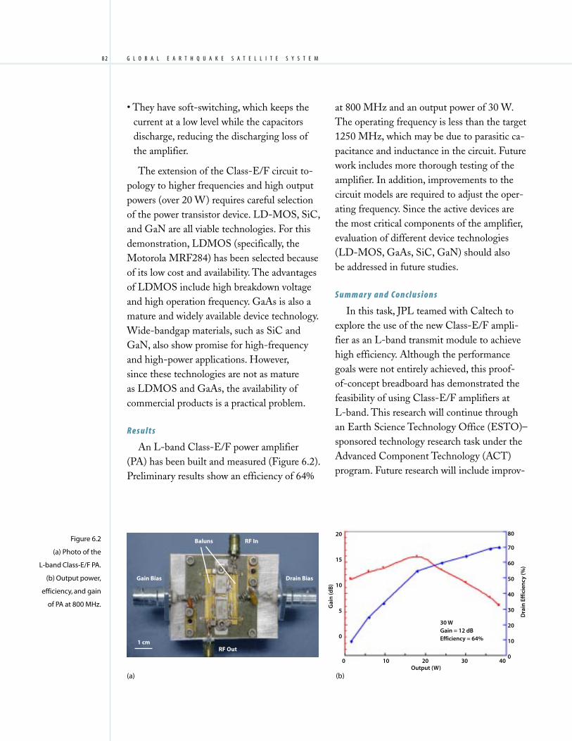
G L O B A L . E A R T H Q U A K E . S A T E L L I T E . S Y S T E M8 2

• They have soft-switching, which keeps the

current at a low level while the capacitors

discharge, reducing the discharging loss of

the amplifier.

The extension of the Class-E/F circuit to-

pology to higher frequencies and high output

powers (over 20 W) requires careful selection

of the power transistor device. LD-MOS, SiC,

and GaN are all viable technologies. For this

demonstration, LDMOS (specifically, the

Motorola MRF284) has been selected because

of its low cost and availability. The advantages

of LDMOS include high breakdown voltage

and high operation frequency. GaAs is also a

mature and widely available device technology.

Wide-bandgap materials, such as SiC and

GaN, also show promise for high-frequency

and high-power applications. However,

since these technologies are not as mature

as LDMOS and GaAs, the availability of

commercial products is a practical problem.

R e s u l t s

An L-band Class-E/F power amplifier

(PA) has been built and measured (Figure 6.2).

Preliminary results show an efficiency of 64%

at 800 MHz and an output power of 30 W.

The operating frequency is less than the target

1250 MHz, which may be due to parasitic ca-

pacitance and inductance in the circuit. Future

work includes more thorough testing of the

amplifier. In addition, improvements to the

circuit models are required to adjust the oper-

ating frequency. Since the active devices are

the most critical components of the amplifier,

evaluation of different device technologies

(LD-MOS, GaAs, SiC, GaN) should also

be addressed in future studies.

S u m m a r y a n d C o n c l u s i o n s

In this task, JPL teamed with Caltech to

explore the use of the new Class-E/F ampli-

fier as an L-band transmit module to achieve

high efficiency. Although the performance

goals were not entirely achieved, this proof-

of-concept breadboard has demonstrated the

feasibility of using Class-E/F amplifiers at

L-band. This research will continue through

an Earth Science Technology Office (ESTO)–

sponsored technology research task under the

Advanced Component Technology (ACT)

program. Future research will include improv-

Figure 6.2

(a) Photo of the

L-band Class-E/F PA.

(b) Output power,

efficiency, and gain

of PA at 800 MHz.

(b)(a)Output (W)

20

15

10

5

0

0 10 20 30 40

80

70

60

50

40

30

20

10

0

Dra

in E

ffic

ien

cy (%

)

Gai

n (d

B)

30 WGain = 12 dBEfficiency = 64%

Gain Bias Drain Bias

RF In

RF Out

Baluns

1 cm

8 3

ing the circuit models to better predict the

performance and then demonstrating im-

proved performance at L-band. Ultimately,

through the ACT program, the Class-E/F PA

will be incorporated into a complete high-

efficiency L-band T/R module.

Geosynchronous SAR Antenna Study

Future advanced SAR concepts, such as the

one being studied by GESS for a geosynchro-

nous SAR mission, require very large antenna

apertures with full 2-D beam-steering capa-

bility. This class of antennas requires apertures

on the order of several hundreds of square

meters transmitting 60 kW of RF power.

For this class of mission to be feasible and

affordable, the antenna mass and stowed vol-

ume must be low enough to fit into an exist-

ing launch vehicle. Antenna mass densities

must be reduced by an order of magnitude

(20 kg/m2 to less than 2 kg/m2).

Several notional concepts were developed

for a geosynchronous SAR mission and two

were studied in some detail. The first concept

is to deploy this system using autonomous,

reconfigurable panels. Here we envision using

an array of hexagonal panels that can be as-

sembled in space to form arrays of differing

geometries. Therefore, the same basic antenna

element can be manufactured in large volumes

on the ground and then assembled in space in

the desired configuration. These autonomous

antenna panels would be completely self-con-

tained each with its own spacecraft avionics

and solar arrays. A detailed study of this con-

cept was conducted for the National Recon-

naissance Office (NRO) under the Director’s

Innovation Initiative (DII) program. The sec-

ond concept under consideration for the geo-

synchronous SAR system is a large deployable

hexagonal antenna with centralized (rather

than distributed) spacecraft bus components,

as described in Chapter 4. The advantage of

this concept is that a single launch vehicle can

deploy the entire array. The autonomous panel

concept would require multiple launches to

deploy an antenna of the size required for

GESS.

A design study was completed of the geo-

synchronous SAR antenna based on the large

deployable antenna concept to identify key

technology drivers for such a system. First,

several antenna architectures were evaluated.

Once the antenna architecture was selected,

a study of the signal generation, distribution,

and transmit/receive architecture was con-

ducted to optimize for low mass, low power,

and maximum performance. Antenna struc-

tures and deployment were also studied.

Based on these design and technology trades,

the antenna mass, power, and cost were esti-

mated. The design was then used in a Team X

exercise to assess overall mission feasibility.

This section summarizes the results of the

antenna design study.

A n t e n n a R e q u i r e m e n t s a n d Pe r f o r m a n c e

The geosynchronous SAR mission design

concept was presented in Chapter 4. The

driving requirements of the radar antenna are

presented in Table 6.3. For a large 30-m aper-

ture antenna and 2-D beam scanning capa-

bility, mass, cost, and complexity are major

factors to be considered in selecting the

antenna architecture. Because the required

amount of beam scan is 8° and possibly

greater for other future systems, only array

concepts are considered for wide-angle beam

scanning needs.

Three array concepts were considered for

performance trade-off: distributed phased

array, reflectarray, and array lens. The distrib-

TECHNOLOGYT E C H N O L O G Y . S T U D I E S

G L O B A L . E A R T H Q U A K E . S A T E L L I T E . S Y S T E M8 4

uted phased array approach has graceful deg-

radation in performance with very little risk of

a single-point failure. Also, by using mostly

corporate-feed power division, the array is

able to achieve adequate RF bandwidth where

more than 10% bandwidth can be achieved.

The reflectarray and lens arrays do not require

complicated beamformers (power dividers)

but have limited bandwidth and require a

high power TWTA. Using distributed T/R

modules would be the more feasible and

reliable approach to achieving the very high

transmit power. The simplicity of the re-

flect-array and array lens approaches cannot

overcome the bandwidth advantage of the dis-

tributed phased array. Because the 6.5% band-

width is an essential requirement of the radar

system, the more complex distributed phased-

array approach is selected.

One of the most constrained aspects of the

array architecture is the element location. The

element locations will determine the overall

sidelobe and grating lobes of the antenna.

From the standpoint of complexity, it is

desirable to minimize the number of elements.

However, insufficient element density causes

the appearance of grating lobes and reduced

gain when the beam is scanned. In order to

minimize the element density while maintain-

ing the required suppression of grating lobes,

a triangular grid is used. By arranging the

elements on the nodes of a triangular grid,

slightly greater (as compared to rectangular

grid) element spacing can be used. The maxi-

mum spacing that will meet the grating lobe

requirements is 0.9 λ, which is 21.4 cm at the

center frequency. Suppression of grating lobes

also requires that each element has its own

phase shifter. A 4-bit phase shifter quantiza-

tion should suffice to achieve the required

beam pointing resolution and sidelobe level.

To reduce the impact of phase shifter losses

on system performance, each element is also

fed by its own T/R module, which contains a

low-noise amplifier (LNA), a PA, and control

circuitry to ensure signal gain on the antenna

element side of the phase shifter. An alterna-

tive architecture includes a T/R module (PA

and LNA) at each subarray and only a phase

shifter at every element. This architecture

requires low-loss phase shifters. The “fully-

populated” architecture delivers better perfor-

mance but at a higher mass and cost. For this

study, we have selected the fully-populated ar-

chitecture with one T/R module per element.

In order for the 30-m antenna aperture to

be stowed and fit into a several-meter launch

vehicle fairing, the antenna’s membrane aper-

ture must be separated into several sections

of rollable and foldable structures. Because

of the separation of structures and folding of

membranes, gaps where there are no radiating

elements (up to 10 cm wide) will be formed

between membranes. In addition, because

of the particular deployment mechanism

Table 6.3

Geosynchronous

SAR antenna

requirements.

PAR A M E T E R R E Q U I R E M E N T

Frequency 1.25 GHz

Bandwidth 80 MHz (6.5%)

Aperture Size 30 m × 30 m

RF transmit power 60 kW

Duty cycle (PW*PRF) 20%

Beam scan ±8° or more

Polarization Single linear vertical

Sidelobe level –30 dB

Cross-pol level –25 dB

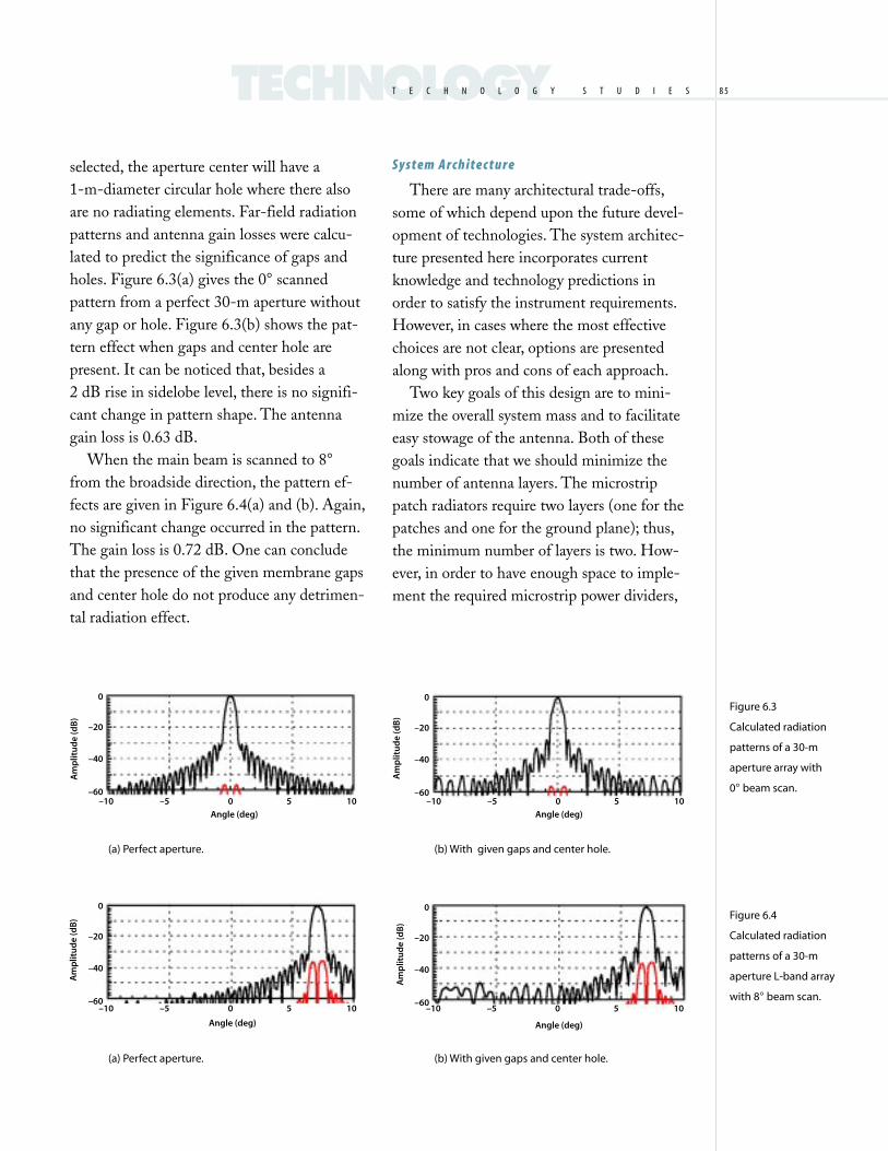
8 5

selected, the aperture center will have a

1-m-diameter circular hole where there also

are no radiating elements. Far-field radiation

patterns and antenna gain losses were calcu-

lated to predict the significance of gaps and

holes. Figure 6.3(a) gives the 0° scanned

pattern from a perfect 30-m aperture without

any gap or hole. Figure 6.3(b) shows the pat-

tern effect when gaps and center hole are

present. It can be noticed that, besides a

2 dB rise in sidelobe level, there is no signifi-

cant change in pattern shape. The antenna

gain loss is 0.63 dB.

When the main beam is scanned to 8°from the broadside direction, the pattern ef-

fects are given in Figure 6.4(a) and (b). Again,

no significant change occurred in the pattern.

The gain loss is 0.72 dB. One can conclude

that the presence of the given membrane gaps

and center hole do not produce any detrimen-

tal radiation effect.

Sy s t e m A r c h i t e c t u r e

There are many architectural trade-offs,

some of which depend upon the future devel-

opment of technologies. The system architec-

ture presented here incorporates current

knowledge and technology predictions in

order to satisfy the instrument requirements.

However, in cases where the most effective

choices are not clear, options are presented

along with pros and cons of each approach.

Two key goals of this design are to mini-

mize the overall system mass and to facilitate

easy stowage of the antenna. Both of these

goals indicate that we should minimize the

number of antenna layers. The microstrip

patch radiators require two layers (one for the

patches and one for the ground plane); thus,

the minimum number of layers is two. How-

ever, in order to have enough space to imple-

ment the required microstrip power dividers,

Figure 6.3

Calculated radiation

patterns of a 30-m

aperture array with

0° beam scan.

TECHNOLOGYT E C H N O L O G Y . S T U D I E S

(a) Perfect aperture. (b) With given gaps and center hole.

Angle (deg)

Am

plit

ud

e (d

B)

Angle (deg)

Am

plit

ud

e (d

B)

–10 –5 0 5 10–10 –5 0 5 10

(a) Perfect aperture.

0

–20

–40

–60

Am

plit

ud

e (d

B)

Angle (deg)

–10 –5 0 5 10

Figure 6.4

Calculated radiation

patterns of a 30-m

aperture L-band array

with 8° beam scan.

(b) With given gaps and center hole.

Am

plit

ud

e (d

B)

Angle (deg)

0

–20

–40

–60–10 –5 0 5 10

0

–20

–40

–60

0

–20

–40

–60

G L O B A L . E A R T H Q U A K E . S A T E L L I T E . S Y S T E M8 6

a third layer is required. Each layer is con-

structed of 40-µm-thick polyimide dielectric

material, such as Kapton®, with copper met-

allization. In order to satisfy the skin depth

requirements at L-band, the copper must be

at least 5 µm thick. However, other require-

ments such as DC power distribution, heat

dissipation, and radiation shielding may

require that the metallization be thicker in

some places.

There are two reasonable places to put the

T/R modules: on the inner ground-plane layer

or on the outer layer with the patch radiators.

In order to minimize the number of intercon-

nections, it is advantageous to place the T/R

modules on the layer with the patches. From a

thermal management perspective, it is best to

place the T/R modules on the ground plane

layer. This allows heat to be spread over the

entire ground plane, increasing radiating area.

However, each T/R module must then be

connected to the patch, which would require

over 15,000 interconnections, decreasing

reliability and making assembly difficult and

costly. A promising approach is to place the

T/R module on the inner layer, as above but

using a noncontacting method, such as

coupled lines or apertures, to feed the T/R

modules and the patches. This is superior

from a mechanical and reliability perspective

but may incur substantial RF losses, thereby

degrading power efficiency and system per-

formance. Because of the substantial advan-

tages of this approach, it merits further

investigation.

Because of the large size and operating

bandwidth of the antenna, true time delays

(TTD) are required for proper beam forma-

tion. If phase delays alone are used, a reduc-

tion in gain and increased grating lobes would

occur. It is impractical to apply a time delay to

every element, so instead, the full array is bro-

ken up in to subarrays of reasonable size and

each subarray has a time delay applied to it.

Additionally, each element within the subarray

contains a controllable phase delay. The full

array and subarray design is illustrated in

Figure 6.5.

There are a total of 61 TTD subarrays. The

size of the time-delayed subarray was chosen

to minimize the degradation of antenna gain

caused from grating lobes. Separation of the

antenna into subarrays also facilitates signal

distribution. Each of these TTD subarrays is

composed of 36 groups of seven elements

(defined as subarrays) arranged in a hexagonal

pattern. All 252 elements in the subarray are

driven by a single digital transceiver. The digi-

tal transceiver receives digital waveform data

from a central controller and converts it to an

analog waveform with the appropriate time

delay and is distributed to the 252 elements

with T/R modules and phase shifters. Re-

ceived power from each element is combined

in the microstrip divider/combiner networks

so that a single L-band analog received signal

reaches the digital transceiver. This signal is

then digitized and the resulting data is sent

back to a central processor/controller (CPC)

for final beamforming. The array system

architecture is shown in Figure 6.6, which

illustrates the interconnection of the CPC,

the TTD subarrays, the T/R modules, and

radiating elements.

As previously noted, true time delay is

required for proper beam formation. This

can be achieved in either analog or digital

circuitry. Analog time-delay circuitry consists

of switched time delays that are implemented

in transmission lines or optical fibers. Because

of the line lengths involved, these delays are

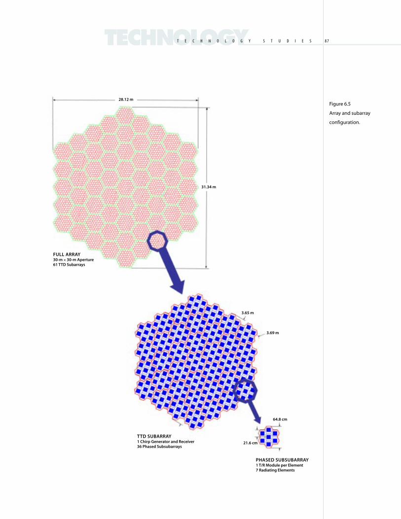
8 7

Figure 6.5

Array and subarray

configuration.

TECHNOLOGYT E C H N O L O G Y . S T U D I E S

PHASED SUBSUBARRAY1 T/R Module per Element7 Radiating Elements

FULL ARRAY30-m × 30-m Aperture61 TTD Subarrays

TTD SUBARRAY1 Chirp Generator and Receiver36 Phased Subsubarrays

3.65 m

3.69 m

21.6 cm

64.8 cm

31.34 m

28.12 m

G L O B A L . E A R T H Q U A K E . S A T E L L I T E . S Y S T E M8 8

difficult to miniaturize. Therefore, the ap-

proach chosen for this design is to implement

the time delays digitally. The major challenge

is developing a low cost method of integrating

optical fibers with the membrane and reliable

connection of fibers to the electronics. Also,

because of the high radiation environment,

radiation-tolerant fibers must be used.

The architecture of the T/R module is

conventional in the sense that it contains a

power amplifier, low-noise amplifier, phase

shifter, programmable attenuator, and control

circuitry. Because of the high average transmit

power of the array, it is essential that the

power amplifiers be as efficient as possible.

Class-E and Class-F amplifiers with over

90% efficiency at 50 MHz have been demon-

strated and efficiencies of 70% at L-band are

predicted. This is an area of ongoing research

of great interest for both radar and communi-

cations applications. A separate activity was

undertaken in the GESS study to demonstrate

an L-band high-efficiency Class-E/F power

amplifier for use in the T/R module, although

it wasn’t assumed in this system design.

While the architecture of the T/R module

is conventional, its packaging is not. In order

to successfully mount T/R modules on a thin

membrane and maintain the ability to fold

and roll it, the modules must have a low mass

and a small footprint. Also, reliable and low-

cost attachment techniques are required. This

requires highly integrated mixed-signal elec-

tronics. In order to reduce the mass of the

modules, radiation shielding must be mini-

mized. This requires the use of highly radia-

tion-tolerant semiconductor technologies.

Figure 6.6

Array system

architecture.Digital Data

Network

61 DigitalTransceivers

To 36-way MicrostripCorporate Feed

36-way MicrostripCorporate Feed

Microstrip7-way Divider

Patch Radiator

252 Elements

FULL ARRAY

TTD SUBARRAY

PHASED SUBARRAY

DigitalTransceiver

DigitalTransceiver

Solid-StateRecorder

Controller

BeamformingProcessor

T/R

Mo

du

le

T/R

Mo

du

le

T/R

Mo

du

le

DataDownlink

T/R

Mo

du

le

Patch Radiator

8 9

Another challenging aspect of such a large

and powerful array radar is generating and

distributing electrical power. Power is gener-

ated by a skirt of flexible solar cells that wrap

around the cone and at the edge of the array.

Power is then fed inward from the perimeter

of the array. In order to minimize ohmic

losses in the power distribution systems,

100 V was chosen for the distribution voltage.

Voltages greater than 100 V run a substan-

tially increased risk of arcing, while lower

voltages will increase ohmic losses. Since the

electronics in the T/R module and digital

transceivers require lower voltages, voltage

conversion is required.

Heavy copper wire attached to the mem-

brane causes unwanted mechanical stresses

and additional integration problems. Since

achieving low-loss transmission requires a

certain conductor cross-sectional area, we

can minimize the thickness of conductors by

maximizing the surface area that they cover.

The ultimate extension of this approach is to

feed the power through a thin copper sheet

on the interior membrane layer. The sheet

can be coated with copper on both sides, with

one side being the power plane and the other

side the ground plane. One danger of this ap-

proach is that a short circuit caused by dam-

age to the membrane may disrupt the power

source for the entire array. An approach to

mitigate this risk is to divide the power plane

into small cells, each connected to its neigh-

bors by fusible links. This concept requires

further study.

S t r u c t u r a l / M e c h a n i c a l

A structural system concept for deploy-

ment of the large antenna and integrated solar

arrays was formulated. This included several

trade studies on various deployable and inflat-

able booms and sizing of the structural mem-

bers (vertical and horizontal booms). A study

of system packaging, membrane management,

deployment, and tensioning was conducted.

A finite-element model was assembled and

used in a preliminary structural analysis. The

results of these studies were used to estimate

the overall system mass and launch volume.

The design was then used in a Team X exer-

cise to assess overall mission feasibility. The

results of the overall geosynchronous SAR

mission design were presented in Chapter 4.

The horizontal booms deploy, support, and

tension the membrane antenna aperture. The

self-rigidizable spring-tape-reinforced (STR)

inflatable booms of 10-inch diameter were

selected for this application for high stiffness

and low mass. Other high-stiffness, light-

weight booms, including those deployed by

mechanical means, are also suitable. The axi-

ally deployed booms must be very stiff to

maintain aperture flatness. We have baselined

the AEC-Able ADAM mast for this applica-

tion since it has SRTM heritage. Able is cur-

rently developing an improved high-stiffness

mast that will reduce the linear mass density

to 1/8 of the SRTM mast and increase the

stowed packaging efficiency by a factor of two

while maintaining equivalent strength, stabil-

ity, and stiffness. This advancement in tech-

nology will simplify the packaging of the

geosynchronous SAR antenna and increase

mass and launch volume margins.

M e m b r a n e A p e r t u r e P a c k a g i n g

Membrane management was studied to

identify a feasible method of packaging and

deploying the antenna. The membrane an-

tenna and the integrated ring-shaped solar

array together form a dodecagon. Each of the

TECHNOLOGYT E C H N O L O G Y . S T U D I E S

G L O B A L . E A R T H Q U A K E . S A T E L L I T E . S Y S T E M9 0

twelve sides of this dodecagon has a length of

19 meters. To package this dodecagon, it will

be first divided by twelve radially extended

fold lines and then be packed by a fold-and-

roll method. The folding part of this packing

method involves the sequential origami

folding steps exemplified in Figures 6.7(a)

through (d).

The folded stack height can be reduced by

increasing the number of rings in the folding

pattern while using the same folding ap-

proach. A four-ring folding will reduce the

stack height to around 5.2 m. Although fur-

ther reduction of stack height can be achieved

by using even more rings, it may present other

difficulties in packing the membrane aperture.

Also, it is important that the RF design be

made compatible with the fold lines as dis-

cussed previously. To stow for launch, the

folded-up membrane stack will be rolled

around the 1-m-diameter central mandrel

that is also the canister housing the stowed

upper ADAM mast.

C o n c l u s i o n s

While the implementation of a large-aper-

ture, high-power, true time delay (TTD) ra-

dar array on flexible membrane presents many

architectural challenges, none of the obstacles

appear insurmountable. A key focus area for

further research is interconnect technology.

Lightweight, low-loss, membrane-compatible

interconnects for RF, and data and power dis-

tribution must be developed. Furthermore,

these interconnects must be highly reliable

and easily manufactured. Continued research

into membrane compatible electronics is also

required. The ultimate goal is a low-cost,

high-reliability process for producing highly

integrated, radiation-hardened, mixed-signal

circuits and attaching them reliably to a mem-

Figure 6.7

Antenna folding

procedure.

(a)

(b)

(c)

(d)

9 1

brane. This technology is critical for imple-

mentation of the GESS radar and would also

enable many other large aperture radar con-

cepts. Membrane antenna technology has

been demonstrated with several successful

ground demonstrations. Future research must

address improved element feeding techniques

such as slot-coupled to replace bulky feed-

probes. This will result in a much less complex

and easier to manufacture design that can

stow much more compactly. The antenna

structures can implement either mature me-

chanically deployable structures or the emerg-

ing technology of inflatable/rigidizable

structures. The first few modes of the system

are governed mainly by the stiffness of the

horizontal booms. Preliminary analysis of the

in-space dynamics of the deployed flight sys-

tem indicates that the fundamental frequency

is greater than 0.2 Hz using inflatable boom

technology, which is well within the capability

of typical spacecraft attitude control systems.

The primary challenge is maintaining accept-

able antenna flatness, and addressing calibra-

tion and metrology techniques to correct for

surface deformation in the array.

Technology Roadmap

W h a t a r e t h e c h a l l e n g e s ?

We have described a number of advanced

SAR mission concepts. For the near-term

missions (LEO and LEO+), there is little

technology development required. Evolution-

ary advances in technology to reduce instru-

ment mass and power will lead to incremental

improvements in performance. However, to

enable the most ambitious GESS mission

concepts, such as the geosynchronous SAR

constellation, revolutionary new technologies

are essential. The antenna is the dominant

component of the radar system and with the

increasing demands for higher resolution,

higher sensitivity, targetability, and coverage,

the antenna aperture becomes very large, re-

quiring a complicated distributed active array

architecture. The array architecture presents

many system-level design and integration

challenges. Since thousands of T/R modules

are required, reducing the mass, power, and

cost of these modules will be very beneficial.

In addition, signal distribution (RF, control,

power) is very complex and low-cost inter-

connect technologies are required to interface

with the modules. Also for the large array,

advanced techniques such as digital

beamforming and TTD steering may be

required. Adaptive methods to compensate

for deformation in the array flatness will also

need to be addressed. These system issues

require a very complicated antenna. For such

a large aperture to fit within existing launch

vehicles, membrane antenna technology

would likely be employed rather than con-

ventional rigid panels. This is a major tech-

nical undertaking.

Inflatable membrane antennas have been

an area of research over the past several years,

with several engineering prototypes developed

to demonstrate that inflatable structures can

be used to deploy and stretch flat membrane

antenna apertures with good RF performance

(Huang et al., 1998). Recent focus on inflatable

structures has been to develop self-rigidizing

technologies and methods to control deploy-

ment. Approaches to properly tension the

membranes to maintain flatness and precise

layer separation is also an area of focus. Al-

though inflatable membrane antennas have

been successfully demonstrated, these anten-

nas have not yet addressed the very compli-

cated problem of integrating electronics

within the aperture. Nor can the existing

TECHNOLOGYT E C H N O L O G Y . S T U D I E S

G L O B A L . E A R T H Q U A K E . S A T E L L I T E . S Y S T E M9 2

systems be scaled to antennas of the size re-

quired for GESS. Mechanically deployed

structures are far more mature than inflatables

and have the advantage of high stiffness and

stability; however, they do not have the high

packing efficiency of inflatable structures.

Trade-off studies indicate that as the structure

length grows beyond 50 m, inflatable tech-

nologies may be advantageous. For GESS,

both inflatable and deployable structures are

candidates.

Besides the mechanical complications of

constructing a large-aperture membrane SAR,

the integration of the large number of T/R

modules and other electronics within the

membrane antenna (reliably and cost effec-

tively) is also a major challenge. Since the ulti-

mate goal is to keep the weight and stowed

volume of the antenna small, conventionally

packaged T/R electronics are not appropriate.

Furthermore, attaching a large packaged com-

ponent to a thin-film membrane also presents

reliability concerns. Therefore, our vision in-

cludes embedding or attaching unpackaged

chips directly to the membrane structure.

The current state-of-the-art T/R modules

typically use three or four chips in a packaged

hybrid microcircuit. A fundamental goal is to

integrate all the T/R electronics onto a single

chip. This will minimize the total part count

and will result in overall reductions in module

cost, assembly cost, and interconnect costs,

while increasing reliability. This is particularly

significant when tens of thousands of T/R

modules are required.

Since the chip is not packaged (at least not

in the same way a conventional T/R module is

packaged), the radiation shielding of the chip

becomes a serious issue. Because the chip is

on a membrane, the heat dissipation from the

T/R is also challenging. New membrane ma-

terials with better heat conductivity are

needed for passive cooling of the electronics.

At high power levels, active cooling methods

such as micromachined heat pipes or similar

technologies may be required. These difficul-

ties are mitigated when very high-efficiency

T/R modules are used.

As advanced (lower TRL) technologies

such as thin-film organic electronics mature,

the possibility of printing some portions of

the T/R electronics (i.e., passive components,

phase shifters, sensors, etc.) directly onto the

membrane may become possible. This would

greatly simplify the complexity and construc-

tion of the antenna and may lead to a substan-

tially lower production cost, which is key to

a viable SAR constellation mission.

C u r r e n t Te c h n o l o g y I nve s t m e n t

NASA is actively working to develop the

technologies required for large membrane

antennas. Figure 6.8 and Table 6.4 show

the roadmap for this effort. Currently two

NASA programs, Code Y’s ACT program

and Code R’s Advanced Measurements and

Detection program, are sponsoring this effort.

The GESS geosynchronous SAR antenna

architecture study has been used to establish

the technology requirements and roadmap

for the long-term SAR missions. The near-

term goal is to demonstrate a fully functional

2 × 8 element antenna subarray by 2004. The

demonstration will combine some of the key

technologies that we have been developing to

ensure that the system as a whole is functional

before more effort is spent on increasing the

TRL of the technologies in use. Internal

R&D funding is also supporting an indepen-

dent task to develop a single-chip MMIC

T/R module, which will ultimately replace

the current five-chip modules.

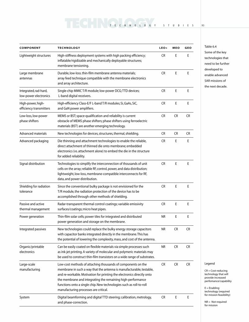
9 3TECHNOLOGYT E C H N O L O G Y . S T U D I E S

Table 6.4

Some of the key

technologies that

need to be further

developed to

enable advanced

SAR missions of

the next decade.

CO M P O NE N T T E C H N O LO G Y LEO+ ME O G E O

Lightweight structures High-stiffness deployment systems with high packing efficiency; CR E E

inflatable/rigidizable and mechanically deployable structures;

membrane tensioning.

Large membrane Durable, low-loss. thin-film membrane antenna materials; CR E E

antennas array feed technique compatible with the membrane electronics

and array architecture.

Integrated, rad-hard, Single-chip MMIC T/R module; low-power DCG; TTD devices; CR E E

low-power electronics L-band digital receivers.

High-power, high- High-efficiency Class-E/F L-band T/R modules; Si, GaAs, SiC, CR E E

efficiency transmitters and GaN power amplifiers.

Low-loss, low-power MEMS or BST; space-qualification and reliability is current CR CR CR

phase shifters obstacle of MEMS phase shifters; phase shifters using ferroelectric

materials (BST) are another emerging technology.

Advanced materials New technologies for devices, structures, thermal, shielding. CR CR CR

Advanced packaging Die thinning and attachment technologies to enable the reliable, CR E E

direct attachment of thinned die onto membrane; embedded

electronics (vs. attachment alone) to embed the die in the structure

for added reliability.

Signal distribution Technologies to simplify the interconnection of thousands of unit CR E E

cells on the array; reliable RF, control, power, and data distribution;

lightweight, low-loss, membrane-compatible interconnects for RF,

data, and power distribution.

Shielding for radiation Since the conventional bulky package is not envisioned for the CR E E

tolerance T/R module, the radiation protection of the device has to be

accomplished through other methods of shielding.

Passive and active Radar-transparent thermal control coatings; variable emissivity CR E E

thermal management surfaces/coatings; micro heat pipes.

Power generation Thin-film solar cells; power tiles for integrated and distributed NR E E

power generation and storage on the membrane.

Integrated passives New technologies could replace the bulky energy storage capacitors NR CR CR

with capacitor banks integrated directly in the membrane. This has

the potential of lowering the complexity, mass, and cost of the antenna.

Organic/printable Can be easily coated on flexible materials via simple processes such NR CR CR

electronics as ink-jet printing. A variety of molecular and polymeric materials may

be used to construct thin-film transistors on a wide range of substrates.

Large-scale Low-cost methods of attaching thousands of components on the CR CR CR

manufacturing membrane in such a way that the antenna is manufacturable, testable,

and re-workable. Motivation for printing the electronics directly onto

the membrane and integrating the remaining high-performance

functions onto a single chip. New technologies such as roll-to-roll

manufacturing processes are critical.

System Digital beamforming and digital TTD steering; calibration, metrology, CR E E

and phase-correction.

Legend

CR = Cost-reducingtechnology that willprovide increasedperfomance/capability

E = Enablingtechnology (requiredfor mission feasibility)

NR = Not requiredfor mission

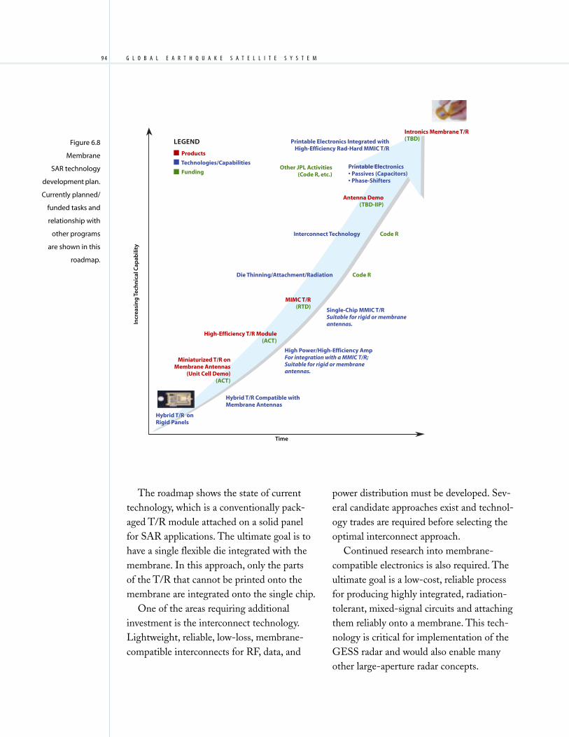
G L O B A L . E A R T H Q U A K E . S A T E L L I T E . S Y S T E M9 4

The roadmap shows the state of current

technology, which is a conventionally pack-

aged T/R module attached on a solid panel

for SAR applications. The ultimate goal is to

have a single flexible die integrated with the

membrane. In this approach, only the parts

of the T/R that cannot be printed onto the

membrane are integrated onto the single chip.

One of the areas requiring additional

investment is the interconnect technology.

Lightweight, reliable, low-loss, membrane-

compatible interconnects for RF, data, and

power distribution must be developed. Sev-

eral candidate approaches exist and technol-

ogy trades are required before selecting the

optimal interconnect approach.

Continued research into membrane-

compatible electronics is also required. The

ultimate goal is a low-cost, reliable process

for producing highly integrated, radiation-

tolerant, mixed-signal circuits and attaching

them reliably onto a membrane. This tech-

nology is critical for implementation of the

GESS radar and would also enable many

other large-aperture radar concepts.

Figure 6.8

Membrane

SAR technology

development plan.

Currently planned/

funded tasks and

relationship with

other programs

are shown in this

roadmap.

LEGEND

Products

Technologies/Capabilities

Funding

Printable Electronics Integrated withHigh-Efficiency Rad-Hard MMIC T/R

Intronics Membrane T/R(TBD)

Other JPL Activities(Code R, etc.)

Printable Electronics• Passives (Capacitors)• Phase-Shifters

Antenna Demo(TBD-IIP)

Interconnect Technology

Die Thinning/Attachment/Radiation

Code R

Code R

MIMC T/R(RTD)

Single-Chip MMIC T/RSuitable for rigid or membraneantennas.

High Power/High-Efficiency AmpFor integration with a MMIC T/R;Suitable for rigid or membraneantennas.

Hybrid T/R Compatible withMembrane Antennas

Miniaturized T/R onMembrane Antennas

(Unit Cell Demo)(ACT)

Hybrid T/R onRigid Panels

High-Efficiency T/R Module(ACT)

Incr

easi

ng

Tec

hn

ical

Cap

abili

ty

Time

9 5

A R T H Q U A K E S C I E N C E I S P O I S E D

to capitalize on a revolutionary capability for observing

global crustal deformation. The concurrent improvements

in seismic monitoring networks, high-performance

computing, and geodetic measurement of crustal defor-

mation have yielded significant advances in knowledge

of fault behavior and crustal stress during the past

decades. A major leap forward will be enabled with the

ability to monitor crustal deformation with high tempo-

ral and spatial resolution. That capability will extend the

observational spectrum into the realm of transient and

aseismic deformation. These fast but seismically quiet

deformation processes, which are at present poorly

understood components of the strain budget, are key

to developing a complete understanding of earthquake

physics. Community models of earthquake physics and

seismic hazards, developed in a data-rich environment,

will rapidly evolve in response to the data. These new

models are expected to yield future earthquake

forecasts of useful dimensions that will feed decision-

support tools to mitigate losses from future large

earthquakes.

The Global Earthquake Satellite System study responds

to the clearly articulated need within the solid-Earth

science community for dense surface deformation data.

It is a detailed implementation plan in alignment with

the recommendations of the SESWG, and charts the

course for NASA to make major contributions to the

interagency EarthScope program, while broadening

those goals to a global scope. In the GESS study, we

explored the requirements space for various compo-

nents of an integrated system, but focused our mis-

sion architecture studies on systems that deliver

high-accuracy, high-resolution surface deformation

using InSAR. Detailed science requirements were gath-

ered from the wider community to guide the studies.

The major conclusion of the architecture studies is

that a constellation of InSAR satellites is needed to

address the requirements for monitoring a spectrum

of steady and transient deformation processes. To

ensure the ability to access any area on the surface

of the Earth within 24 hours would require two LEO

satellites in orbits above 1000 km. A few MEO or GEO

satellites would be equivalent to many spacecraft in

LEO and would fully characterize the known transient

processes such as postseismic relaxation, slow earth-

quakes, creep events, and accelerated slip, with full

global coverage. It is expected that new discoveries of

even faster processes than are recognized today will

accrue as crustal deformation measurements extend

into the subdaily time scale. The spectrum of transient

deformation processes known at present includes

The 20-Year Plan

E

9 5

G L O B A L . E A R T H Q U A K E . S A T E L L I T E . S Y S T E M9 6

surface deformation due to ground water storage, and

hence, the hydrologic cycle. Thus, the opportunity for

synergistic interaction of hydrology and tectonics, espe-

cially with regard to liquefaction susceptibility, is

an exciting area of interdisciplinary research that is

an added benefit of the high spatially and temporally

resolved deformation measurements.

The GESS integrated science and technology plan

shown on the opposite page maps the desired

scientific knowledge to observational and modeling

requirements and to technology investments needed to

achieve the vision. Measurements from LEO orbits are

within reach at present. Higher vantage points, such

as MEO or geosynchronous, require investments in

inflatable, deployable antennas and structures, high-

efficiency lightweight electronics, and new processing

schemes to account for varying atmospheric and iono-

spheric conditions during the long integration times

required to achieve the synthetic aperture from a

slowly moving platform. These investments should be

made now to ensure that NASA is ready to respond to

the wealth of new discoveries that will be returned

by a near-term LEO InSAR constellation.

LEO/LEO+ CONSTELLATION

Incr

easi

ng

Tem

po

ral a

nd

Sp

atia

l Res

olu

tio

nIn

crea

sin

g L

on

g-T

erm

Mea

sure

men

t A

ccu

racy

Near Term

Short-Term (Monthly),Targeted (Fault System)

GEO/MEO CONSTELLATIONContinuous Global Coverage

GEO/MEOPATHFINDER MISSION

LEO/LEO+ PATHFINDER MISSION

Understanding

Improved Hazard Assessments

Disaster Response

Far Term

G E S S R o a d m a p

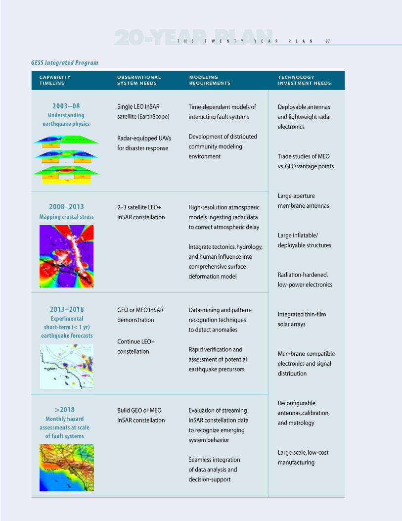
9 7

Deployable antennas

and lightweight radar

electronics

Trade studies of MEO

vs. GEO vantage points

Large-aperture

membrane antennas

Large inflatable/

deployable structures

Radiation-hardened,

low-power electronics

Integrated thin-film

solar arrays

Membrane-compatible

electronics and signal

distribution

Reconfigurable

antennas, calibration,

and metrology

Large-scale, low-cost

manufacturing

Time-dependent models of

interacting fault systems

Development of distributed

community modeling

environment

Build GEO or MEO

InSAR constellation

>2018Monthly hazard

assessments at scaleof fault systems

2013–2018Experimental

short-term (< 1 yr)earthquake forecasts

2008–2013Mapping crustal stress

2003–08Understanding

earthquake physics

Single LEO InSAR

satellite (EarthScope)

Radar-equipped UAVs

for disaster response

2–3 satellite LEO+

InSAR constellation

GEO or MEO InSAR

demonstration

Continue LEO+

constellation

Evaluation of streaming

InSAR constellation data

to recognize emerging

system behavior

Seamless integration

of data analysis and

decision-support

Data-mining and pattern-

recognition techniques

to detect anomalies

Rapid verification and

assessment of potential

earthquake precursors

High-resolution atmospheric

models ingesting radar data

to correct atmospheric delay

Integrate tectonics, hydrology,

and human influence into

comprehensive surface

deformation model

CAPABI LI T Y OBSERVAT IONAL MODELING TECHNOLO GYTIMELINE SYSTEM NEEDS REQUIREMENTS INVESTMENT NEEDS

GESS Integrated Program

20-YEAR PLANT H E . T W E N T Y . Y E A R . P L A N

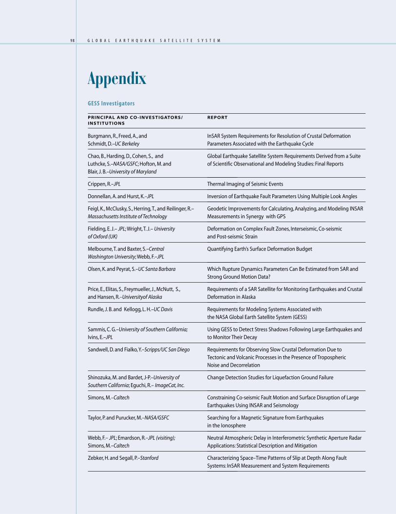
9 8

Burgmann, R., Freed, A., andSchmidt, D.–UC Berkeley

Chao, B., Harding, D., Cohen, S., andLuthcke, S.–NASA/GSFC; Hofton, M. andBlair, J. B.–University of Maryland

Crippen, R.–JPL

Donnellan, A. and Hurst, K.–JPL

Feigl, K., McClusky, S., Herring, T., and Reilinger, R.–Massachusetts Institute of Technology

Fielding, E. J.– JPL; Wright, T. J.– Universityof Oxford (UK)

Melbourne, T. and Baxter, S.–CentralWashington University; Webb, F.–JPL

Olsen, K. and Peyrat, S.–UC Santa Barbara

Price, E., Elitas, S., Freymueller, J., McNutt, S.,and Hansen, R.–Universityof Alaska

Rundle, J. B. and Kellogg, L. H.–UC Davis

Sammis, C. G.–University of Southern California;Ivins, E.–JPL

Sandwell, D. and Fialko, Y.–Scripps/UC San Diego

Shinozuka, M. and Bardet, J-P.–University ofSouthern California; Eguchi, R.– ImageCat, Inc.

Simons, M.–Caltech

Taylor, P. and Purucker, M.–NASA/GSFC

Webb, F.– JPL; Emardson, R.–JPL (visiting);Simons, M.–Caltech

Zebker, H. and Segall, P.–Stanford

InSAR System Requirements for Resolution of Crustal DeformationParameters Associated with the Earthquake Cycle

Global Earthquake Satellite System Requirements Derived from a Suiteof Scientific Observational and Modeling Studies: Final Reports

Thermal Imaging of Seismic Events

Inversion of Earthquake Fault Parameters Using Multiple Look Angles

Geodetic Improvements for Calculating, Analyzing, and Modeling INSARMeasurements in Synergy with GPS

Deformation on Complex Fault Zones, Interseismic, Co-seismicand Post-seismic Strain

Quantifying Earth’s Surface Deformation Budget

Which Rupture Dynamics Parameters Can Be Estimated from SAR andStrong Ground Motion Data?

Requirements of a SAR Satellite for Monitoring Earthquakes and CrustalDeformation in Alaska

Requirements for Modeling Systems Associated withthe NASA Global Earth Satellite System (GESS)

Using GESS to Detect Stress Shadows Following Large Earthquakes andto Monitor Their Decay

Requirements for Observing Slow Crustal Deformation Due toTectonic and Volcanic Processes in the Presence of TroposphericNoise and Decorrelation

Change Detection Studies for Liquefaction Ground Failure

Constraining Co-seismic Fault Motion and Surface Disruption of LargeEarthquakes Using INSAR and Seismology

Searching for a Magnetic Signature from Earthquakesin the Ionosphere

Neutral Atmospheric Delay in Interferometric Synthetic Aperture RadarApplications: Statistical Description and Mitigation

Characterizing Space–Time Patterns of Slip at Depth Along FaultSystems: InSAR Measurement and System Requirements

P R I N C I PA L A N D C O - I N V E S T I G ATO R S / R E P O RTI N S T I T U T I O N S

GESS Investigators

G L O B A L . E A R T H Q U A K E . S A T E L L I T E . S Y S T E M

Appendix

9 9

GESS Science Definition Team

Chair: Carol A. Raymond

Jet Propulsion Laboratory,California Institute of Technology

Douglas Burbank

University of California, Santa Barbara

Benjamin F. Chao

NASA Goddard Space Flight Center

Andrea Donnellan

Jet Propulsion Laboratory,California Institute of Technology

Alan Gillespie

University of Washington

Thomas L. Henyey

University of Southern California

Thomas Herring

Massachusetts Institute of Technology

Thomas Jordan

University of Southern California

Donald L. Turcotte

Cornell University

Mary Lou Zoback

U.S. Geological Survey

APPENDIXT E A M S . A N D . R E F E R E N C E S

References

Bawden, G., W. Thatcher, R. S. Stein, K. W. Hudnut, and G. Peltzer,

Tectonic contraction across Los Angeles after removal of

groundwater pumping effects, Nature, 412, 812–815, 2001.

Burgmann, R., A. M. Freed, and D. Schmidt, InSAR system

requirements for resolution of crustal deformation param-

eters associated with the earthquake cycle, 10 pp., Final

Report, GESS Requirements Definition Study, JPL Contract

1232377, 2002.

Chao, B. F., S. C. Cohen, D. J. Harding, M. Hofton, J. B. Blair, and

S. B. Luthcke, Global Earthquake Satellite System requirements

derived from a suite of scientific observational and modeling

studies: Final reports, 24 pp., Final Report, GESS Requirements

Definition Study, 2002.

Crippen, R., Thermal Imaging of Seismic Events, 6 pp.,

Final Report, GESS Requirements Definition Study, 2002.

DeLouis, B., P. Lundgren, J. Salichon, and D. Giardini, Joint

inversion of InSAR and teleseismic data for the slip history of

the 1999 Izmit (Turkey) earthquake, Geophys. Res. Lett., 27,

3389–3392, 2000.

Feigl, K., S. McClusky, T. Herring, and R. Reilinger, Geodetic im-

provements for calculating, analyzing and modeling INSAR

measurements in synergy with GPS, 9 pp., Final Report, GESS

Requirements Definition Study, JPL Contract 1233102, 2002.

Fielding, E. J. and T. J. Wright, Deformation on complex fault

zones, interseismic, co-seismic and post-seismic strain,

Final Report, GESS Requirements Definition Study, 2002.

Fenoglio, M. A., M. J. S. Johnston, and J. Byerlee, Magnetic and

electric fields associated with changes in high pore pressure

in fault zones: application to the Loma Prieta ULF emissions,

J. Geophys. Res., 100, 12951–12958, 1995.

Freed, A. M. and J. Lin, Delayed triggering of the 1999 Hector

Mine earthquake by viscoelastic stress transfer, Nature, 411,

180–183, 2001.

Hamza, V. M., Tectonic leakage of fault bounded aquifers

subject to non-isothermal recharge: a mechanism generating

thermal percursors to seismic events, Phys. Earth Plan. Int.,

126, 163–177, 2001.

Hofton, M. A. and J. B. Blair, Detecting vertical ground surface

change using laser pulse correlation, J. Geodyn., 34, 477–489,

2002.

GESS Study Team,Jet Propulsion Laboratory,California Institute of Technology

Carol A. Raymond

Science Lead

Soren Madsen

Radar Lead

Wendy Edelstein

Technology Lead

Jeff Booth

Curtis Chen

Adam Freedman

David Imel

Said Kaki

Yunling Lou

Paul Lundgren

G L O B A L . E A R T H Q U A K E . S A T E L L I T E . S Y S T E M1 0 0

Huang J., M. Lou, A. Feria, and Y. Kim, An inflatable L-band

microstrip SAR array, IEEE AP-S/URSI Symposium, Atlanta,

Georgia, pp. 2100–2103, June 1998.

Ivins, E., personal communication to Carol A. Raymond, 2003.

Johnston, M. J. S., Review of electric and magnetic fields

accompanying seismic and volcanic activity, Surveys in

Geophysics, 18, 441–475, 1997.

Kee, S.D., I. Aoki, and D. B. Rutledge, 7-MHz, 1.1-kW demon-

stration of the new E/F2,odd switching amplifier class, 2001

IEEE MTT-S International Microwave Symposium Digest, 3,

1505–1508, 2001.

Komatitsch, D. and J. Tromp, Spectral-element simulations

of global seismic wave propagation - I. Validation, Geophys.

Jour. Int., 149, 390–412, 2002.

Lienkaemper, J.J., J. S. Galehouse, and R.W.Simpson, Creep

response of the Hayward Fault to stress changes caused by

the Loma Prieta earthquake, Science, 276, 2014–2016, 1997.

Lundgren, P. R., InSAR time series resolution of blind thrust

and surface fault creep, 3 pp., Final Report, GESS Require-

ments Definition Study, 2002.

Madsen, S. N., C. Chen, and W. Edelstein, Radar options for

global earthquake monitoring, IGARSS 04_09_14:00, 2002.

Melbourne, T., S. Baxter, and F. Webb, Quantifying Earth’s

surface deformation budget, 9 pp., Final Report, GESS Require-

ments Definition Study, JPL Contract 1232313, 2002.

Minster, J. B., personal communication to Carol A. Raymond,

2001.

Olsen, K., and S. Peyrat, Which rupture parameters can be

estimated from SAR and strong ground motion data?, 11 pp.,

Final Report, GESS Requirements Definition Study, JPL Contract

1232158, 2002.

Park, S. K., Precursors to earthquakes: Seismoelectromagnetic

signals, Surv. Geophys., 17, 493–516, 1996.

Pollitz,F.F. and I. S. Sacks, Stress triggering of the 1999 Hector

Mine earthquake by transient deformation following the

1992 Landers earthquake, Bull. Seismo. Soc. Amer., 92,

1487–1496, 2002.

Price, E., S. Elitas, J. Freymueller, S. McNutt, and R. Hansen,

Requirements of a SAR satellite for monitoring earthquakes

and crustal deformation in Alaska, 10 pp., Final Report, GESS

Requirements Definition Study, JPL Contract 1232431, 2002.

Pritchard, M., M. Simons, P. Rosen, S. Hensley, and F. Webb,

Geophys. J. Int., 150, 362–376, 2002.

Rundle, J. B. and L. H. Kellogg, Requirements for modeling

systems associated with the NASA Global Earthquake Satel-

lite System (GESS), 25 pp., Final Report, GESS Requirements

Definition Study, JPL Contracts 1232241/1232379, 2002.

Rundle, J. B., L. H. Kellogg, K. F. Tiampo,W. Klein, P. B. Rundle, and

A. Donnellan, Illuminating the relationship between observ-

able data and unobservable dynamics using numerical simu-

lations of a changing Earth, PAGEOPH, submitted, Fall 2002.

Sandwell, D. and Y. Fialko, Requirements for observing slow

crustal deformation due to tectonic and volcanic processes

in the presence of tropospheric noise and decorrelation,

CD-ROM Final Report, GESS Requirements Definition Study,

JPL Contract 1232381, 2002.

Sammis, C. G. and E. Ivins, Using GESS to detect stress

shadows following large earthquakes and to monitor their

decay, 17 pp., Final Report, GESS Requirements Definition

Study, JPL Contract 1235152, 2002.

Shinozuka, M., B. Mansouri, R. T. Eguchi, and C. K. Huyck,

Change detection studies for liquefaction ground failure:

16 pp., Final Report, GESS Requirements Definition Study

(Part A), JPL Contract 1232166, 2002.

Taylor, P. and M. Purucker, Searching for a magnetic signature

from earthquakes in the ionosphere, 76 pp., Final Report,

GESS Requirements Definition Study, 2002.

Tobita, T., J-P Bardet, and M. Shinozuka, Regional detection of

soil liquefaction susceptibility using SAR, 58 pp., Final Report,

GESS Requirements Definition Study (Part B), JPL Contract

1232166, 2002.

Toda, S., R. S. Stein, and T. Sagiya, Evidence from the AD 2000

Izu islands earthquake swarm that stressing rate governs

seismicity, Nature, 419, 58–61, 2002.

Tomiyasu, K., Conceptual performance of a satellite borne,

wide swath synethic aperture radar, IEEE Transactions on

Geoscience and Remote Sensing, GE-19(2), 108–116, 1981.

Zebker, H. and P. Segall, Characterizing space–time patterns

of slip at depth along fault systems: InSAR measurement and

system requirements, 6pp., Final Report, GESS Requirements

Definition Study, JPL Contract 1232132, 2002.

1 0 0 G L O B A L . E A R T H Q U A K E . S A T E L L I T E . S Y S T E M

JPL 400-1069 03/03