31. methods of determining the excess attenuation
TRANSCRIPT

31. METHODS OF DETERMINING THE EXCESS ATTENUATION
FOR GROUND-TO-GROUND NOISE PROPAGATION
By Stanley H. Guest
NASA George C. Marshall Space Flight Center
and
Bert B. Adams
Lockheed Missiles and Space Company
SUMMARY
Three basic methods of obtaining excess attenuation values for ground-to-ground sound propagation are described for use in various applications. The acquisition of the acoustic data, the selection of usable information, and the influencing meteorological factors are given along with the results. The relative effects of seasonal variation, relative humidity, and temperature a re provided in addition to the nonlinearity effects with distance as were observed from the data. The results obtained from this study can be applied to noise control relating to airport/community problems as well as to any other general noise abatement situation concerning sound propagation over the ground surface.
INTRODUCTION
According to the Federal Aviation Administration, the revenue air passenger miles are expected to increase by 250 percent within the next 10 years. reasonable to expect that the interference of airplane noise with people will also increase proportionately. It is thus apparent that this ever-growing problem must be given serious study.
(See ref. 1.) It is
Because of the increasing complexity of the physical and psychological problems created by the general and continued use of jet engines by both military and civilian agencies, The Federal Aviation Administration instituted what is known as the Interagency Noise Abatement Program in an attempt to find techniques to alleviate as much as possible for as many people as possible at a cost that is within reason, these acoustical problems adversely affecting our environment. The techniques include a combination of three basic approaches to these problems: (1) modifying the sound source (that is, producing quieter jet engines), (2) optimizing the flight path along which the sound is transmitted, and (3) developing a satisfactory airport/community interface, both physically and psychologically.
453

The sound source problem will not be handled in this paper, nor will the interfacing be directly discussed.
The consideration of the transmission path and the variables affecting the sound propagation is a complicated task and would directly impact such aspects as airport plan- ning and layout, residential and commercial land zoning, building code criteria, personnel safety and annoyance factors, test procedures for aircraft certification, and many other considerations which require long- term planning and airport/community interface.
To plan for community activities in relation to large noise sources (jet ports), studies are being made of the behavior of sound as it is propagated from i t s source to a receiver, where both the source and receiver a re at ground level. The substance of this paper is, effectively, a study of far-field attenuation of sound, the results of which can be applied to airport "ground operations" from the landing of the aircraft through the "taxi" phase, passenger pick-up, and so forth, until just after take-off. This period of ground operation can be lengthy and contributes largely to the growing problem of aircraft noise.
CA
CH
EA
N
OBSPLd
OBSPLj
OBSPLk
OBSPLn
OBSPLo
R.H.
Rd
454
SYMBOLS
velocity of sound (vector to Athens), m/sec
velocity of sound (vector to Huntsville), m/sec
excess attenuation including all attenuation of energy in excess of spherical divergence, dB/unit distance
integer
octave band sound pressure level at distance radius Q from source, dB, re 2 x 1 0 - 5 ~ 1 ~ ~
octave band sound pressure level at any position j, dB, re 2 X 10⁻⁵N/m2
octave band sound pressure level at any position k, dB, re 2 X 10⁻⁵N/m2
octave band sound pressure level at position n, dB, re 2 X 10'5N/m2
octave band sound pressure level at a reference position Ro, dB, re 2 x 1 0 - 5 ~ / ~ 2
relative humidity at ground level, percent
distance radius to any microphone more distant than Ro, distance units
distance radius from sound source to microphone position j, distance units Rj
Rk
Rn distance radius to position n, distance units
distance radius from sound source to microphone position k, distance units
distance radius to reference microphone closest to source, distance units R O
TG temperature at ground level, OC
WA
WH
E-l mean value
(T standard deviation
$2 average of squared values
wind velocity toward Athens, m/sec
wind velocity toward Huntsville, m/sec
TEST SETUP AND DISCUSSION OF PROBLEM
Because of its large test-stand facilities, where large rocket engines and boosters are static tested under varied weather conditions, the George C. Marshall Space Flight Center has ready-made high-energy sound sources which are ideal for this type of study: the S-IC, booster for the Saturn V space vehicle; the S-IB, booster for the Saturn IB space vehicle; and the F-1 rocket engine, the single-engine element of the S-IC booster. To make extensive studies of the acoustic energy propagation by these sound sources, a Land Acoustical Monitoring System (LAMS) has been permanently installed at the center. Only the installation of this Land Acoustical Monitoring System was necessary to take advantage of the following already existing factors at the Marshall Space Flight Center for acoustic studies: first, the large sound source; second, long data samples to be obtained over an extended test duration; third, a sound source invariant with time or test; fourth, a large number of tests and data measurements; and fifth, extensive meteorolog- ical survey information at the actual location of the test. (The Aerospace Environment Division, Aero-Astrodynamics Laboratory, Marshall Space Flight Center, makes sys- tematic studies of meteorological conditions,)
The LAMS system consists of two radial lines of transducers located in two direc- tions from the test stands. (See fig. 1.) The first line of transducers consists of
455

29 microphones along a 36-km line at an azimuth of approximately 310° (k3O) in the direc- tion of Athens, Alabama, and the second consists of 22 microphones along an 18-km line at an azimuth of approximately 45O (k6O) in the direction of Huntsville, Alabama. The microphones are mounted on telephone poles a t 40 feet above the local temain at a median separation distance of 1.5 km (Athens LAMS) and 0.9 km (Huntsville LAMS). The three static test stands a r e located in a triangular pattern at a maximum distance of less than 1.5 km apart. Figure 1 also shows the relative positions of the microphones and test stands with the ground elevation along each radial LAMS line. It can be seen that the elevation is relatively constant (k25-foot variations) along the Athens LAMS and along the first 15 km of the Huntsville LAMS. (Only four microphones are placed at higher eleva- tions and they are at the greatest distance from the source.)
The ground cover for the Athens LAMS is estimated to be 80-percent open fields (farms, pastures, grassland) with intermittent trees and hedgerows. The Huntsville LAMS is approximately 60- to 70-percent open country with wooded areas, partly decid- uous and partly evergreen. No other quantitative information is currently available concerning the physical makeup of the soil o r the impedance characteristics typical of the ground and its cover. For both lines, it can only be estimated that the tree height averages 20 to 30 feet and the grass cover is about 6 inches. No bodies of water intervene.
The acoustic data used in this study were acquired from among 79 tests during the period from June 1965 to January 1967 by using the static tests of the Saturn V booster (214.5 dB sound power level; all sound power levels referenced to watt), the S-IB booster (204 dB sound power level), and the F-1 rocket engine (204.5 dB sound power level).
DATA ACQUISITION SYSTEM
The data acquisition system, basically designed by Bolt Beranek and Newman, Inc., of Boston, Massachusetts, consisted of 51 permanently located microphones on 40-foot telephone poles. The Chesapeake NM 135 and a modified model of increased sensitivity, along’with several Shure microphones, were calibrated before each test by a hand-held calibrator (diaphragm type) producing a single frequency signal (100 Hz). The micro- phones were again checked, this time remotely, just before static test firing of the engines, by an insert voltage technique. The remote check was made on the assumption that the spectral response characteristics remained flat, after the laboratory calibration, over the frequency range from 1 Hz to 2000 Hz. Remote attenuator settings (5, 10, and 30 dB), available for each microphone, were used when prior prediction of the sound field indicated that radical levels were expected. This prediction was based on the velocity- of-sound profiles containing vector wind, temperature, and humidity factors.
456
6

The output from each microphone was amplified and fed to an FM modulator and then to the base station at the George C. Marshall Space Flight Center (MSFC) over land- lines. The signal was directly recorded on a 14-track recorder for data processing. The accuracy quoted on the data-acquisition system was &2 dB for 95-percent confidence level from 1 Hz to 1000 Hz. The background noise was also recorded just before data acquisition to prevent use of any anomalous electrical noise or any interfering physical noise which might be recorded from any of the microphones.
The data reduction from the magnetic tape to a digital form was conducted on an automatic octave band data system. The data were printed on cards for computer use and were also plotted for visual inspection. The time-history record was observed from several transducers and an analysis was made of an acceptable portion of the test data. An averaging time of 50 seconds was used for tests of sufficient duration and an aver- ageing time of 20 seconds for others. (The average test duration was 75 seconds.)
From the statistical considerations, concerning only the conversions from magnetic tape to digital form, the averaging appeared to be quite acceptable. On the assumption of a normal probability distribution, a confidence level of 99.5 percent had less than *1 dB spread for the 10-Hz center frequency octave band data that were averaged for 20 seconds. The 50-second averaging time yielded less than &0.6 dB spread for the same confidence level and frequency.
The meteorological data (velocity of sound, wind, temperature, and relative humidity as a function of altitude; 79 600 points of information) used in this study were obtained from the facilities of the Marshall Aero-Astrodynamics Laboratory which are located approximately 2 km from the static test stands. These operations a re similar to those of a U.S. weather station in data acquisition, record keeping, and handling of statistics. The equipment facilities and data handling techniques a r e described in reierences 2 and 3. The atmospheric data were obtained from ground level to an altitude of 20 to 50 km. It has been established from these data that, in general, the effects of refraction of sound waves back to the ground plane for distances of approximately 20 km away from the source depend primarily on the existing conditions (velocity profile) at low altitudes, that is, less than 3 kilometers above the ground. To be safe the velocity of sound profiles and vector winds were observed from ground level to an altitude of 5 km.
The atmospheric conditions for all altitudes were acquired by releasing a radio- sonde transducer about 2 minutes before firing time. The radiosonde, tracked by a GMD system, reported position coordinates for determination of winds aloft. The temperature, relative humidity, and position coordinates were reported at 30-second intervals. The wind values, after being smoothed by a seven-point weighted mean technique, were then recorded. The relative humidity was used with the temperature and wind vector infor- mation to produce velocity-of -sound profiles as functions of azimuth angle,
457
The meteorological values given were generally in 150-meter altitude increments. This increment varied slightly because of the rate of change of ascent of the balloon with altitude.
DATA SELECTION AND ANALYSIS I
After the data had been reduced to a usable form (that is, octave band spectra as a function of distance from the source and all the supporting data including the atmospheric conditions), it became obvious that not all the data were applicable to defining the atten- uation caused by the ground surface and its cover. This fact is due to the refractive properties of the layered atmosphere. For example, the atmospheric medium with its layered structure of warmer or cooler air or with winds aloft can alter the sound pres- sure levels on the ground about the source by refracting the energy along-paths not common with that of propagation in an isentropic homogeneous medium. The resultant is seen in the form of sound pressure gradients (with distance) that are not related to those normally found with the loss in proportion to the inverse of the distance and the normal attenuation properties. For cases of energy being returned to the ground, where ray concentration is greater than normal, the gradient is considered to be positive. It may be highly positive for cases where ray paths converge, a caustic o r a focal zone being produced; o r conversely, the gradient may be highly negative, and the energy directed away from the ground plane, again deviating from the normal propagation path considered for a homogeneous isentropic atmosphere. These situations occur in the Marshall data, as they would in any locale where the atmospheric gradients are significant. Thus, to determine the attenuation characteristics associated with the ground plane or the atmos- pheric media, these extraneous effects of atmospheric conditioning must at least be recog- nized. Since the quantitative effects of refraction are very difficult to describe analyti- cally, the data for cases where significant atmospheric gradients were present were elimi- nated. It can only be hoped that the effects of scattering and dispersion due to turbulence will be minimized by the selection of data from tests where wind velocity was relatively low; thus, having many tests, especially for the various field conditions, is necessary for any isolation of the variables involved.
The selection of which tests to use, for cases of nonsignificant refraction conditions, was made on the basis of wind velocity and the velocity-of-sound profile (vector profiles) for each LAMS line. The test data were considered to be acceptable for analysis if the wind speed was less than approximately 5 m/sec (ground level), if the gradient did not exceed 10 m/sec-km (0.010 sec-l) for the gross profile characteristics, and if no addi- tional excessive gradients were observed in the small layer structure of the atmosphere. For example, if the gross characteristic of the velocity-of-sound profile up to 3 km altitude was -5 m/sec-km but had a local additional gradient of *lo m/sec-km over an
458

altitude segment of greater than a half kilometer, then that test was not considered as representative of a nonrefractive atmospheric situation. This local additional gradient change of A 0 m/sec-km was adopted as a general rule for data selection after examining the data and the results of acoustic ray-tracing programs and decibel contour plots with the meteorological data as input. The gross characteristics of the velocity-of -sound profiles observed from the data used in this study are given in table I with the wind vectors (and standard deviations) for the Huntsville and Athens LAMS lines at altitude increments of one-half kilometer. The temperature and the relative humidity at ground level are also given by seasonal periods (summer, May to August; fall, September to November; winter, December to February; spring, March to April). By applying these criteria for limiting the use of data acquired under what are considered to be significantly refractive conditions, the potential number of data points representing values for attenuation in the frequency range from 1 Hz to 1000 Hz was reduced. method I, the data bits were reduced from 943 500 to 61 505. See table 11).
.
(For the first proposed approach,
ANALYSIS METHODS
Several computer programs were written for the IBM 7094 to perform the calcula- tions and data sorting for different analysis methods. The three approaches used are given in the following sections.
Method I
In the first approach al1,acoustic data were corrected for background noise level. For those cases in which the data did not exceed the noise floor by at least 3 dB, the data were rejected. For a single test case, and along a specific LAMS line where a common directivity index was assumed (that is, the directivity index at 310° azimuth was con- sidered to be constant within ~t3O about the line), the octave band sound pressure level for two microphones was assumed to be given by
where OBSPL values a r e the octave band sound pressure levels at any microphone j and k; and Rk are the distances corresponding to any two microphones; and EA(f) is the excess attenuation per octave band, given in dB/distance. The excess attenuation, that is, the attenuation due to the air, the ground cover, or any other cause (excluding divergence) for any octave band, is given as
459

R- OBSPLj - OBSPLk + 20 loglo 2
Rk Rk - Rj
dB/dis tance EA(f) =
If it is assumed that the EA per unit distance is independent of the distance from the source and if this comparison is made for each microphone or combination of micro- phones, - comparisons per octave band are made where N represents the number of microphones which have provided octave band data for that test. (See fig. 2.)
2
By multiplying the EA values for any one test by the number of comparisons used
from that test, that is, (EA)test [ N(N - 1) ltest , summing all such terms for many tests,
and dividing by the total average for the excess attenuation is found.
for all the tests (for a given octave band), a weighted 2
Method I1
The second analytical approach was to acquire the EA values as they were simi- larly obtained by references 4 and 5, among others. The closest microphone was chosen as the reference point and the EA values were then calculated from ever-increasing distances from the reference. (See fig. 2.) From
Rd QBSPLO - QBSPLd = 20 loglo - RO + EA(f)(Rd - Ro)
RO OBSPLO - OBSPLd + 20 loglo - EA(f) = Rd dB/distance
Rd - Ro
where Ro is the radial position of the reference microphone, the closest to the source, and Rd indicates the radial position of the next more distant microphone in sequence.
Method 111
A third approach was used also to look at the EA values in piecewise distance increments, not overlapping increments, over the entire measurement range. (See fig. 2.) The equations were basically the same; only the input was arranged differently.
The excess attenuation is expressed as
460

Rn OBSPLn - OBSPLn+1 + 20 loglo - - IN-' dB/distance K. EA(f) =
Rn+1 - Rn
where Rn is the radius position of any microphone in a sequence and Rn+1 is the next adjacent microphone at a greater distance from the source. All microphones were used together with the adjacent one to form a piecewise description of EA along the propaga- tion path. Thus, the EA per unit distance would be observed in small increments at an ever-increasing distance from the source. This approach indicates any nonlinear effects of attenuation and the position or distance range at which they would occur, that is, because of the sound pressure decreasing with increased distances, or could help in determining whether the turbulence effects, the terrain, or even whether the meteorological conditions of refraction a r e causing the attenuation to appear nonlinear or nonuniform over the measurement field.
Method 111 provides the most information about the EA characteristics with dis- tance along the transmission path since the only averaging used is over the number of tests involved; whereas the other methods involved averaging over long distances and nonuniform sound pressure level gradients.
RESULTS AND DISCUSSION
The methods of handling the acoustic data are varied and should certainly depend on the objective of the researcher. In the literature several forms of analysis are noted; some a r e presented as dependent on the distance from the source (refs. 4 to 8), others are given for use with various distance ranges (refs. 4 and 9), in another approach (ref. 10) the excess attenuation is given as a function of the product of the distance and the frequency, and still other presentations are given as independent of distance (refs. 7, 11, and 12).
The results herein were all acquired from the same se t of data but analyzed in various ways (methods I, 11, and 111 as described) and presented accordingly for use in application to various problems. In the future it is hoped that the complexity of this prob- lem due to the currently inseparable influence of several variables can be reduced. Also the physical phenomena causing the varied interpretations should be separated and more effectively considered. Much more work is to be done with the Marshall data but this work requires a large amount of computer time on a limited basis and therefore will proceed accordingly.
46 1

It is thought that the data acquisition program at Marshall - the large number of measurements from many tests, the detail in the meteorological data, the long sound dura- tions, and long averaging times in conjunction with the stationary high-energy sources - makes these data much more appealing for study than some tests with conditions that are somewhat meagerly described in the literature.
Method I
Results for method I (EA values averaged over all possible combinations of micro- phones, independent of distance) are presented in this section. The EA values derived from this portion of the analysis represent the average attenuation per season (including ground and propagational medium effects) per unit distance over all possible microphone combinations and thus are independent of the distance from the source.
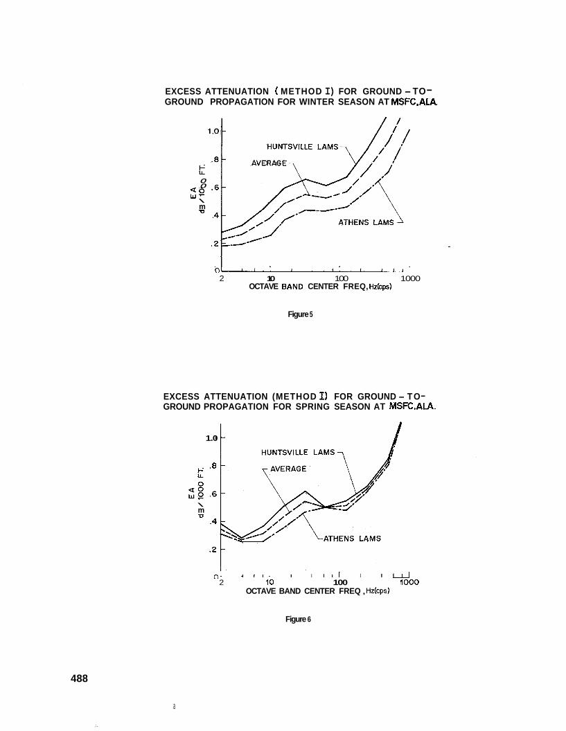
The averaged EA values, computed for each LAMS line, for various seasons (figs. 3 to 6) do not appear to change significantly to merit consideration of the season as a variable in the application of the EA values. From figure 7, however, there appears to be some physically reasonable order to the EA values across the entire frequency range. The highest values of attenuation were observed in the sequence of fall, summer, winter, and spring over most of the frequency range. Since the layer of ground cover has possibly reached a maximum depth in the fall, that is, dropped leaves, highest weed and crop growth, and so forth, the fall season might be of correct order. Likewise the ground cover growth is standing erect and at near maximum height with leaves still on the t rees in the summer and thus possibly implies greater attenuation than is observed with the more barren ground plane of the spring and winter. However, the differences in the values for the four seasons (by chosen date) possibly do not merit concern since the spread of data averages is so small. Reference 5 shows a similar spread of EA values for the sea- sons. The variation is more exaggerated but the ground conditions are possibly quite different in Leningrad, Russia.
The average value of the excess attenuation from method I, including atmospheric and ground effects (constructive and destructive interference is negligible for the fre- quency range and the geometry) is indicated in figure 8 with the plot of the excess attenu- ation values for air. (See ref. 13.) Of notable mention for field data is that the excess attenuation for air (ref. 13) tends to exceed the cumulative effects of classical absorption, the excess attenuation for the air media, the effects of turbulence as a scattering agent, and the absorptive properties of the ground plane and its cover (acting to some degree, on the macroscale, as a layer of sound-absorbing material on a wall) at the higher frequency values of 1000 Hz and above. This comparison, of course, considered the averaged tem- perature and relative-humidity conditions.
462

The effect of relative humidity on the EA values did not appear to be significant; however, only three tests were available for use in the low humidity range and thus the standard deviations for data were larger than for the comparisons using larger test sam- ples. Likewise, the effect of temperature as measured in the ground plane did not corre- late with the EA variations in any discernible order that was incompatible with the sea- sonal order.
The attenuation at the lower frequency range is somewhat more pronounced than has been expected since few EA values are found in the literature for acoustic energy below 30 Hz. The attenuations in this frequency range are significantly greater than can be attributed to the molecular absorption phenomenon for the atmosphere. The small increase in the EA values (fig. 8) in the 50-Hz region is not explainable, other than being related to some ground-cover characteristics (showing a similar trend on Athens and Huntsville LAMS lines) or to the prevalent physical characteristics of the atmosphere.
Method 11
Method 11 made use of a reference microphone in connection with all others to pro- vide EA values for a sequence of ever-increasing propagation distances. (See fig. 2). This method effectively smooths some of the nonuniform EA values noted over the prop- agation path (as found from method HI).
The EA values, as obtained from approximately 3200 data bits, are provided in fig- ures 9 and 10 for only the summer season because of a lesser number of tests available for analysis in the other three seasons. These data also indicate that the nonlinearity of EA with distance is more pronounced for less than 25 000 feet from the source. Beyond 35 000 feet the nonlinearity is not noted in the data. From observing the averages of the EA values per season from method I (fig. 7), it is expected that any seasonal effect still should be of minimal concern.
Figure 11 delineates the comparison of the results of other researchers for approxi- mately the same conditions; however, referenced reports presented very meager informa- tion on the meteorological o r other test conditions. It is noted that there is a spread of the EA values over the entire frequency range. Perhaps the ground conditions were a factor in some of the cases where large differences were observed, but it is also pos- sible that other factors could be responsible for some of the wide variations in results. These factors could include a nonstationary sound source, lack of meteorological data, a small number of measurements, the inclusion of data for extreme atmospheric conditions (winds, velocity profiles, and short test durations and data averaging times), and, in gen- eral, other similar deficiencies in complete, applicable, and accurate data acquisition.
463

Method El
The values of EA, as obtained from piecewise distance increments, are given over the entire measurement range; that is, the EA value between microphones 1 and 2 EAl2 was plotted at the distance midpoint of that increment and EA23 likewise, until all the microphones were used. For several of the octave bands the general results of method 111 compared favorably with the results of method 11. (See figs. 12 and 13 and compare methods 11 and 111 for 500 Hz and 250 Hz.) The other octave band frequency data lacked sufficient statistical accuracy for reporting at this time.
The nonuniformity of the variation of EA values with distance, from method 111, indicates that they do not always fall into a more orderly pattern as derived from method 11 results, since there is extensive inherent averaging with that approach (method II). The nonuniformity of EA with distance is physically due to nonuniformity in the data; that is, the sound pressure levels varied nonuniformly. This variation is due to either actual differences in rates of absorption in each of the increments, effects of refraction in certain local areas (lapse conditions for higher EA values, and rays returning for lower EA values), effects of local winds in certain increments, local ter- rain effects, or other inhomogeneities in the atmosphere. The EA values from method 111, however, tend to be positive in an exaggerated manner when there is even a very local shadow zone. Because of the extreme sensitivity to small sound pressure level changes over small distances, the EA values for method III are not statistically accept- able to merit explicit use in an engineering application to airport noise at this time. Thus these small variations in sound pressure levels distort the average EA values and thus present a problem in acquiring a set of'experimental data from the field corresponding to the theoretical perfect atmosphere and terrain conditions of the laboratory.
This third method would be the most descriptive of the three approaches since it provides the EA values as they exist over each small distance increment and these values are not lost in the averaging process; however, a great number of tests would be required for a statistically acceptable definition of the attenuation features. Thus this method did not produce any usable engineering values even with the relatively large number of tests available.
CONCLUSIONS
In general, the following statewents can be made concerning the analyses of the data by the three methods described herein:
1. Method I - All possible microphone combinations - provides excess attenuation EA values that are low because of weighted averaging resulting from the nonlinearity effects.
464

REFERENCES
1. Sperry, W. C.; Powers, J. 0.; and Oleson, S. K.: Status of the Aircraft Noise Abate- ment Program. Sound and Vib., vol. 2, no. 8, Aug. 1968, pp. 8-21. .
2. Turner, Robert E.; and Schow, Robert R.: MSFC Atmospheric Sounding Station Semiannual Operation Review. MTP-AERO-62-59, NASA George C. Marshall Space Flight Center, 1962.
3. Turner, Robert E .; and Jendrek, Richard A. : Radiosonde Automatic Data Processing System. NASA TM X-53186, 1964.
4. Parkin, P. H.; and Scholes, W. E.: The Horizontal Propagation of Sound F rom a Jet Engine Close to the Ground, at Radlett. J. Sound Vib., vol. 1, no. 1, Jan. 1964, pp. 1-13.
5. Parkin, P. H.; and Scholes, W. E.: The Horizontal Propagation of Sound From a Jet Engine Close to the Ground, at Hatfield. J. Sound Vib. vol. 2, no. 4, Oct. 1965, pp. 353-374.
6. Anon.: Method for Calculating the Attenuation of Aircraft Ground to Ground Noise Propagation During Takeoff and Landing. AIR 923, SOC. Automot. Eng., Mar. 1, 1968.
7 . Dneprovskaya, I. A.; Iofe, V. K.; and Levitas, F. I.: On the Attenuation of Sound as It Propagates Through the Atmosphere. Sov. Phys. - Acoust., vol. 8, no. 3, Jan.- Mar. 1963, pp. 235-239.
8. Ingard, Uno: A Review of the Influence of Meteorological Conditions on Sound Propa- gation. J. Acoust. SOC. Amer., vol. 25, no. 3, May 1953, pp. 405-411.
9. Franken, Peter A.; and Bishop, Dwight E.: The Propagation of Sound From Aircraft Ground Operations. NASA CR-767, 1967.
10. Wiener, Francis M.; and Keast, David N.: Experimental Study of the Propagation of Sound Over Ground. J. Acoust. SOC. Amer., vol. 31, no. 6, June 1959, pp. 724-733.
11. Anon.: Acoustical Considerations i n the Planning and Operation of Launching and Static Test Facilities for Large Space Vehicles. Phase I. BBN 884 (Contract Nas 8-2403), Bolt, Beranek, and Newman, Inc., Dec. 11, 1961.
12. Benson, R. W.; and Karplus, H. B.: Sound Propagation Near the Earth's Surface as Influenced by Weather Conditions. WADC Tech. Rep. 57-353, Pt. I, U.S. Air Force, Mar. 1958. (Available from DDC as AD 130793.)
13. Harris , Cyri l M.: Absorption of Sound in Air Versus Humidity and Temperature. NASA CR-647, 1967.
466

2. Method I serves basically as an approach for recognizing relative EA effects.
3. The EA values for air (molecular absorption) appear to be high for the f re- quency range above 1000 Hz o r 2000 Hz.
4. Seasonal effects on EA values appear to be small.
5. Variations of relative humidity and temperature (ground values) have little effect on EA values.
6. The meteorological effects have a great influence on computed EA values. Supporting data for tes ts a r e mandatory.
7. Methods II and 111 provide comparable results if ground effects are homogeneous and there are no atmospheric refraction cases.
8. Methods 11 and III more nearly provide the EA values for general engineering/ airport use application, The method used should be compatible with the desired objective.
9. The method used fo r determining EA information should be selected on the basis of its providing the desired objective for engineering application.
465

TABLE I.- METEOROLOGICAL CONDITIONS ASSOCIATED WITH
Altitude, m
0 500
1000 1500 2000 2 500
Altitude, m
0 500
1000 1500 2000 2 500 3000
Sound velocity (referenced to ground value)
To Athens To Huntsville
*2 l-l U Q2 l-l 0
0 0 0 0 0 0 16.42 -3.67 1.72 23.67 -4.38 2.11 19.88 -6.79 1.94 62.50 -7.42 2.73 94.08 -9.33 2.65 120.04 -9.75 4.99
139.33 -11.50 2.66 193.4 1 -12.83 5.36 196.58 -13.75 2.74 250.08 -15.00 I 5.00
THE ACOUSTIC DATA (LAMS)
(a) Summer
Wind velocity
To Athens -
Q2
5.91 12.83 14.50 16.75 17.20 18.75 26.25
l-l
0.50 .66 .25 .08 .12
- .29 - .50
U
2.38 3.52 3.79 4.09 4.14 4.32 5.09
To Huntsville
1 p
3 .oo 8.87
12.05 19.75 26.04 21.45 20.45
l-l
-0.16 - .71 -.79
-1.25 -1.79 -2.12 -2.04
U -
1.72 2.88 3.38 4.26 4.78 4.11 4.03
467

TABLE I.- METEOROLOGICAL CONDITIONS ASSOCIATED WITH
THE ACOUSTIC DATA (LAMS) - Continued
Altitude, m
I
Relative humidity,
m/s m/s m/s m/s OC percent WAS WH, CAJ CH, TG’
2000 -3 2 500 -4 3000 -4
L I I
0 0 0
0 500 1000 1500 2000 2 500 3000
0 500 1000 1500 2000 2 500 3000
-~
0 -3 -7
- 10 -3 -11 -3 - 14 0 -17
0 -2 -3 -4 -3 -4 -4
0 -3 -5 -8
-11 - 14 -17
-2 2 0 0 0 -4 -7
-3 -8
-11 - 13 -13 - 10 -9
-
0 -3 -7
- 10 - 13 - 16 - 19
0 0 -3 -9 -3 - 14 -5 - 18 -8 -21 -13 - 19 -17 - 19
S-IB; test 37; June 29, 1966 I
26 78
468
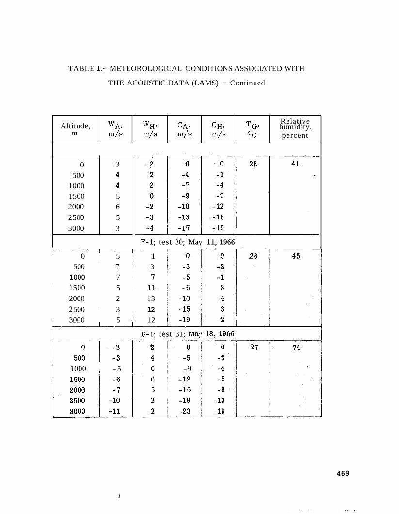
TABLE I.- METEOROLOGICAL CONDITIONS ASSOCIATED WITH
THE ACOUSTIC DATA (LAMS) - Continued
Altitude, m
Relative WA, WH, CA, CH, TG, humidity, m/s m/s m/s m/s OC percent
0 500
1000 1500 2000 2 500 3000
F-1; test 30; May 11, 1966
3 4 4 5 6 5 3
0 5 1 500 7 3 1000 7 7 1500 5 11 2000 2 13 2 500 3 12 3000 5 12
F-1; test 31; Ma!
1000 -5 -9 I I I
469

TABLE I.- METEOROLOGICAL CONDITIONS ASSOCIATED WITH.
THE ACOUSTIC DATA (LAMS) - Continued
Altitude, m
(a) Summer - Continued
Relative wH, CAY CH, TG, humidity,
m/s m/s m/s 4 s OC per cent WA,
0 500 1000 1500 2000 2 500 3000
-4 -6 -7 -9 -9 -9 -9
3 0 0 29 68 2 2 0 0 -1 -2
-2 I -2 1
-6 -6 -9 -8
- 13 -11 - 16 -15 - 16 - 15 - 18 - 18
0 500 1000
~ 1000 -3 -7
1 2 4
1500 2000 2 500 3000
3 2 2 4
0 -7
- 10 - 14 - 19 - 24 -25
1500 2000 2500
47 0
1 -4 -11 2 -6 -13 2 -9 -15
3000 4 - 10 - 13
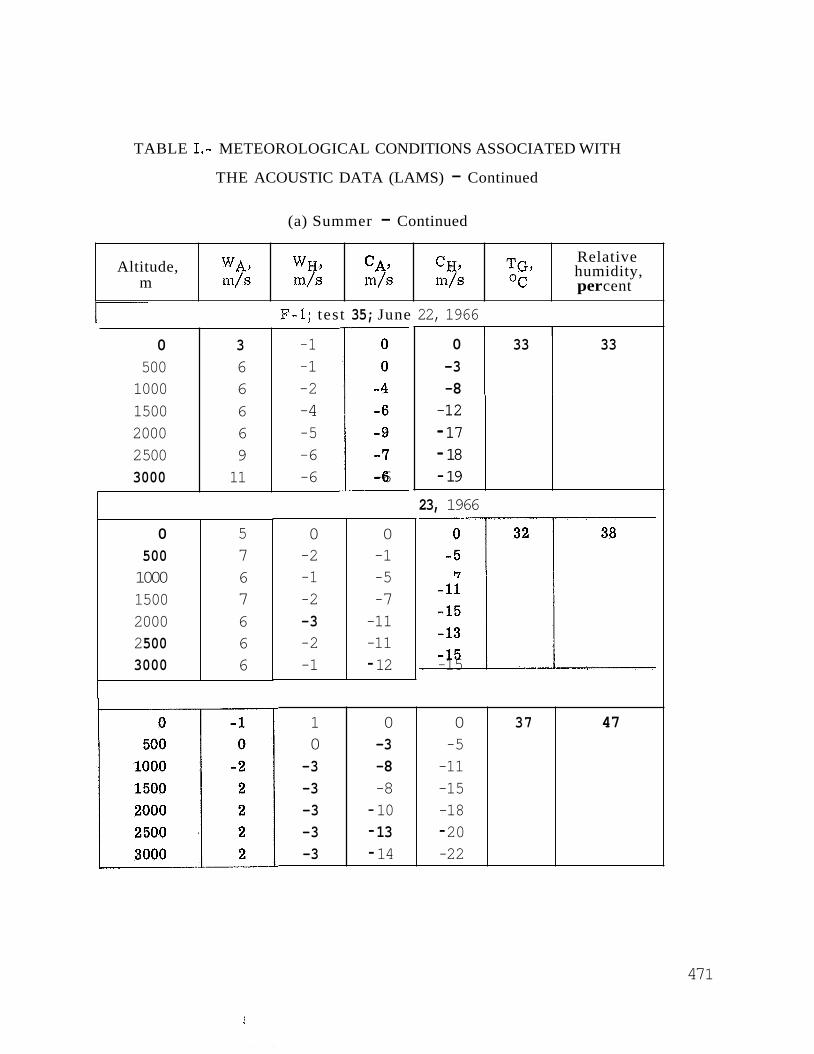
TABLE I.- METEOROLOGICAL CONDITIONS ASSOCIATED WITH
Altitude, WA, WH, CAP CH, TG, m m/s m/s m/s m/s OC
THE ACOUSTIC DATA (LAMS) - Continued
Relative humidity, per cent
(a) Summer - Continued
0 3 500 6 1000 6 1500 6 2000 6 2 500 9 3000 11
-1 -1 -2 -4 -5 -6 -6
I 0 -3 -8
33 33
0 -2 -1 -2 -3 -2 -1
i -6
0 -1 -5 -7
-11 -11 - 12
F-1; test 35; June 22, 1966 1 I
0 500 1000 1500 2000 2 500 3000
5 7 6 7 6 6 6
1 0 0 0 -3 -5 -3 -8 -11 -3 -8 -15 -3 - 10 -18 -3 - 13 - 20 -3 - 14 -22
-12 - 17 - 18 - 19
37 47
-12 - 17 - 18 - 19
23, 1966
~
~ -15 ~ -15
47 1
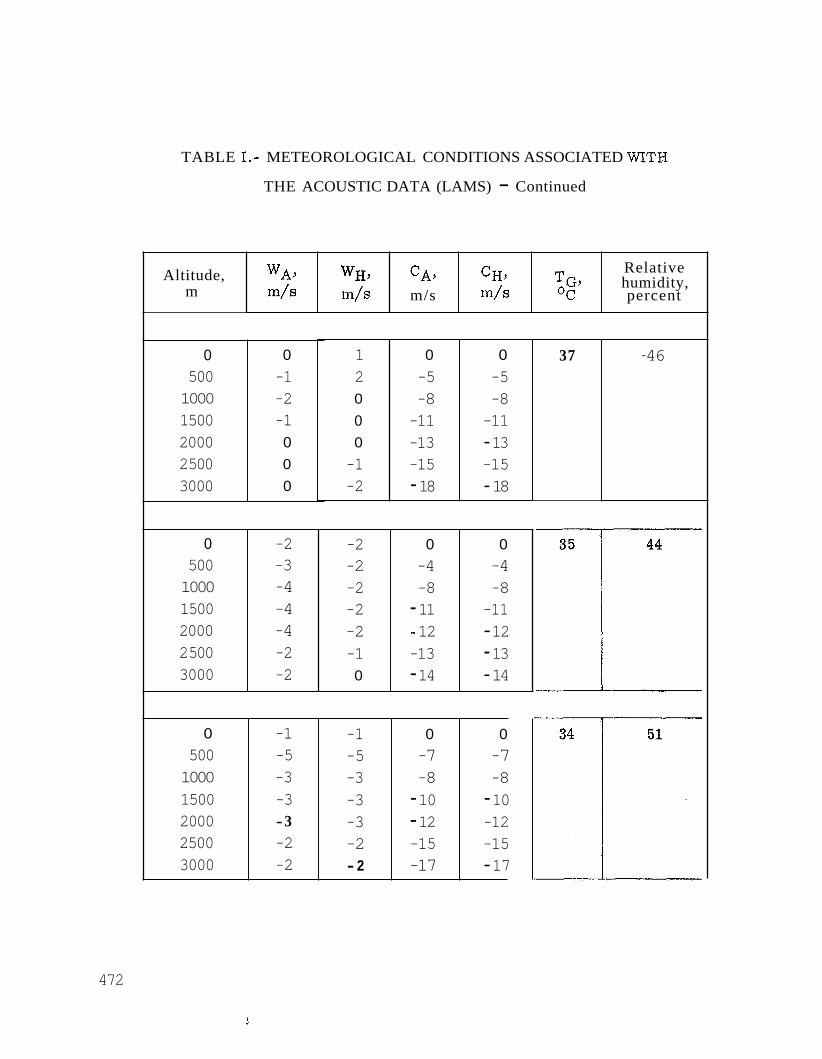
TABLE I.- METEOROLOGICAL CONDITIONS ASSOCIATED WITH
THE ACOUSTIC DATA (LAMS) - Continued
WA, 4 s
Altitude, m
Relative TG, humidity,
m/s m/s m/s OC percent WHY CA, CH,
0 500 1000 1500 2000 2 500 3000
1 2 0 0 0 -1 -2
0 0 -5 -5 -8 -8
-11 -11 -13 - 13 -15 -15 - 18 - 18
0 -1 -2 -1 0 0 0
0 -2 500 -3 1000 -4 1500 -4 2000 -4 2 500 -2 3000 -2
-2 0 0 -2 -4 -4 -2 -8 -8 -2 - 11 -11 -2 - 12 - 12 -1 -13 - 13 0 - 14 - 14
0 -1 500 -5 1000 -3 1500 -3 2000 -3 2500 -2 3000 -2
37
-1 0 0 -5 -7 -7 -3 -8 -8 -3 - 10 - 10 -3 - 12 -12 -2 -15 -15 - 2 -17 - 17
-46
1 1
1
472
1

TABLE I.- METEOROLOGICAL CONDITIONS ASSOCIATED WITH
THE ACOUSTIC DATA (LAMS) - Continued
Altitude, WA9 m m/s
(a) Summer - Continued
Relative humidity,
m/s m/s m/s OC percent WH, CA, CH9 TG,
0 500
1000 1500 2000 2 500 3000
2 0 3 0 2 -2 2 -4 4 -4 4 -2 2 -2
0 -3 -7 -9 -9
- 12 - 15
0 -6 -8
- 10 -15 - 18 - 20
F-1; test 45; July
40 0 500
1000 1500 2000 2 500 3000
0 500
1000 1500 2000 2 500 3000
-2 0 -3 0 -4 0 -5 1 -5 -1 -3 -2 -3 -2
0 -7
-11 - 15 - 16 -17 -19
0 -2 -4 -4 -5 -5 -4
0 -4 -9
- 13 -15 - 16 - 17
13, 1966
0 0 0 -1 -6 -4 -1 - 10 -7 0 - 14 - 10
-2 - 17 - 14 -3 - 19 -17 -3 -21 -20
39 43
41
473

474
CA9 4 s m/s
Altitude, WA, WH? m m/s
TABLE I.- METEOROLOGICAL CONDITIONS ASSOCIATED WITH
THE ACOUSTIC DATA (LAMS) - Continued
Relative CH, TGY humidity, m/s OC percent
(a) Summer - Continued
0 -6 -8
- 12 - 16 -17 -15
34
F-1; test 47; July 25, 1966
0 -6 -8
- 12 - 16 -17 -15
0 500
1000 1500 2000 2 500 3000
34
F-1; test 48; August 5, 1966
0 0 500 0
1000 2 1500 3 2000 2 2500 1 3000 0
0 -1 -1 -3 -3 -1 0
0 -2 -5 -7 -8 -9 -9
0 0 0 0 0 500 1 2 -3 -3
1000 0 2 -6 -6 1500 -1 4 -11 -6 2000 -1 5 - 14 -8 2 500 -1 3 - 15 -11 3000 -1 1 - 16 -15
33 53
49; August 9, 1966
51 51

TABLE I. - METEOROLOGICAL CONDITIONS ASSOCIATED WITH
THE ACOUSTIC DATA (LAMS) - Continued
WH, CA, CH., m m/s m/s m/s m/s
Altitude, WA,
(a) Summer - Concluded
Relative TG? humidity, OC percent
0 -3 -3 0 0 27 500 -3 -7 -4 -7
1000 -2 -5 -6 -9 1500 0 -3 -6 -9 2000 0 -1 -7 -7 2 500 -3 -1 - 10 -8 3000 -5 0 - 13 -8
39
F-1; test 65; June 14, 1967 I 1 I
0 1 3 0 0 33 34 500 1000 1500 2000 2 500 3000
2 1 1 2 3 4 -
0 -2 -3 -3 -5 -7
-4 -8
-11 - 12 - 14 - 14
-6 - 10 - 14 -17 -21 -25
47 5
TABLE I. - METEOROLOGICAL CONDITIONS ASSOCIATED WITH
THE ACOUSTIC DATA (LAMS) - Continued
Altitude,
(b) Fall
Wind velocity
To Athens To Huntsville
Y m
0 ~
0 500
1000 1500 2000 2500 3000
0.49 2.72 2.03 2.97 4.27 4.27 4.76
Altitude, m
0 500
1000 1500 2000 2 500 3000
0.2 3.80 4.0 2.40 9.40
11.6 27.8
q2 0.4
10.0 7.4
17.8 39.4 61.8 77.4
-0.20 1.40 1.20
.40
.60
.80
-0.40 -1.60 -1.80 -3.00 -4.60 -6.60 -7.40
0.40 1.36 1.60 1.50 3.00 3.31
1.40
I - I
5.08
0 +2 Y 1c,2
0 20.8 51.4 94.0
159.0 225.8 309.4
~~
Sound velocity (referenced to ground value) I
P
0 -4 .O -7.0 -9.2
-11.8 -14.2 -17.0
I To Huntsville
0 2.19 1.55 3.06 4.44 4.92 4.52
0 0 6.2 -2.2
25.4 -4.6 51.8 -6.8 57.8 -7.0 64.6 -7.8 90.4 -8.8
0
0 1.17 2.06 2.36 2.97 1.94 3.60
47 6

TABLE I.- METEOROLOGICAL CONDITIONS ASSOCIATED WITH
THE ACOUSTIC DATA (LAMS) - Continued
(b) Fall - Continued
F-I; test 52; September 13, 1966
0 500
1000 1500 2000 2 500 3000
-1 -1 -1 0 0
-3 -3
0 -4 -6 -8 -9
- 12 - 15
0 -3 -7
- 10 - 10 -9 -9
F-I; test 54; October 26, 1966
29 57
0 500
1000 1500 2000 2 500 3000
-1 -3 -3 - 3 -1 -1 -1
0 2 0 0
-1 -2 -4
0 -4 -7 -6 -6 -6
0 -1 - 5 - 5 -8 -9
22 20
I -9 I -13 1 I I I I I
F-I; tes t 71; October 19, 1967
0 500
1000 1500 2000 2 500 3000
0 -6 - 5 -8
-12 -13 -13
0 -1 -1 -2 -4 -4 -4
0 -8
-10 -1 5 -19 -20 -21
29
477

478
Altitude m
TABLE I. - METEOROLOGICAL CONDITIONS ASSOCIATED WITH
THE ACOUSTIC DATA (LAMS) - Continued
Relative WAY wH7 cA7 CH, TG7 humidity m/s 4 s m/s m/s OC percent
(b) Fall - Concluded
0 500 1000 1500 2000 2500 3000
0 0 -1 -4 -6 -9
- 12
F-I; test 73: November 16, 1967
0 -2 -6 -8
-11 -15 -20
0 -2 -1 -2 -3 -5 -7
Averasre
15 16
20.4 I 27.4

TABLE I. - METEOROLOGICAL CONDITIONS ASSOCIATED WITH
THE ACOUSTIC DATA (LAMS) - Continued
cr
0 2.48 3.43 5.71 7.42 7.91 6.97
(c) Winter
@ 0 12.2 3.8 31.8 15.8 19.8 32.4
Altitude m
Wind velocity
To Athens To Huntsville
0 500 1000 1500 2000 2 500 3000
Wind velocity
To Athens To Huntsville Altitude m
cr EL cr EL
0 2.2 -0.6 1.36 1.8 0.2 1.33 500 10.6 - .6 3.20 17.80 1.4 3.98 - 1000 29.2 -2.8 4.62 23.60 .4 4.84 1500 67.6 -4.4 6.94 25.80 2.2 4.58 2000 116.4 -6.4 8.68 29.2 4.0 3.63
128.2 -7.4 8.57 4 5.40 6.2 2.64 3000 147.6 9.2 7.93 63.2 1 7.6 2.33 . 2500 I
Altitude, m
0 500 1000 1500 2000 2 500 3000
10.6 - .6 3.20 17.80 1.4 3.98 - 29.2 -2.8 4.62 23.60 .4 4.84 67.6 -4.4 6.94 25.80 2.2 4.58 116.4 -6.4 8.68 29.2 4.0 3.63 128.2 -7.4 8.57 4 5.40 6.2 2.64 147.6 9.2 7.93 63.2 7.6 2.33
Sound velocity (referenced to ground value) I
To Athens
$J2 0 14.0 63.6 136.6 213.8 293.6 417.2
E-l
0 -2.8 -7.2 -10.2 -12.6 -1 5.2 -19.2
I To Huntsville
EL
0 -1.8 -5.2 -4.6 -3.0 -2.6 -2.8
cr
0 2.99 3.31 3.26 2.61 3.61 4.96
479

TABLE I.- METEOROLOGICAL CONDITIONS ASSOCIATED WITH
Altitude, m
THE ACOUSTIC DATA (LAMS) - Continued
Relative TG’ humidity,
m/s 4 s m/s 4 s OC percent
WA, WH, CA, cH,
0 500
1000 1500 2000 2 500 3000
S-IC; test 16; February 17, 1966
-2 -2 -4 -6 -8 -8
-10
10 -2
-4 -6 -4 0 6
11
38 - 0 -4 -8
-12 -13 -1 5 -18
0 500
1000 1500 2000 2500 3000
0 -7
-11 - 10 -5 0
-3
-2 2 0 0 13 38 -2 7 -4 -1 -8 7 -12 - 2
-14 6 -1 9 -3 -20 6 -25 -4 -20 6 -29 - 7 -20 5 -31 -9
2 500 3000
2 3 2 5
1500 2000 3
~ -5 - 5 -T” -5
480
40

TABLE I. - METEOROLOGICAL CONDITIONS ASSOCIATED WITH
Relative TG, humidity,
m m/s m/s m/s m/s OC percent Altitude, WA, WH, CA, CH,
-
THE ACOUSTIC DATA (LAMS) - Continued .
1 0 4 4 4 4 4 8 3 10
-3 9 2 11
(c) Winter - Concluded
0 1 -2 -3 -5
-14 -8
0 500 1000 1500 2000 2 500 3000
S-IB; test 32; January 17, 1966
3 3 2 0
. -1 -2 -4
0 50 0 1000 1500 2000 2 500 3000
0 500 1000 1500 2000 2 500 3000
S-IB; test 40; November 16, 1966
0 18 60 1
-2 0 2 1
-2
F-1; test 24; April 27, 1966
0 5 8
11 12 14 14
0 -3 -7
-11 -13 -17 -22
48 1

TABLE I. - METEOROLOGICAL CONDITIONS ASSOCIATED WITH
+2 8.16 44.83 71.5 99.33 113.33 14 1.0 150.33
482
E-l
1.83 5.83 7.83 9.33 10.0 11.0 11.33
Altitude, m
0 500 1000 1500 2000 2 500 3000
6.5 23.3 16.16 15.83 27.50 52.00 78.0
THE ACOUSTIC DATA (LAMS) - Continued
(dl Spring
Wind velocity
0.16 .oo
- 1.50 -2.83 -4.50 -6.66 -8.0
To Athens
0 8.17 10.50 20.50 26.17 29.17 45.00,
0 .83 .16
- 1.17 -2.25 -2.83 - 5.00
0
2.54 4.83 3.73 2.80 2.70 2.76 3.74
0 500 1000 1500 2000 2500
To Huntsville
0 0 0 18.67 -3.33 2.75 63.00 -7.67 2.04 129.66 -11.33 1.14 206.66 -14.33 1.15 378.00 -19.33 2.08
3000
3.50 3.65 4.47 4.69
520.00 -22.67 2.46
I Sound velocity (referenced to ground value) Altitude, 1 ~2 , ~ , To Athens m To Huntsville
+2 I E-l (T
0 2.73 3.24 4.38 4.59 4.60 4.47

TABLE I. - METEOROLOGICAL CONDITIONS ASSOCIATED WITH
THE ACOUSTIC DATA (LAMS) - Continued
I
Relative humidity,
m/s m/s m/s m/s OC percent Altitude, WA, wH, C A, CH, TG,
m -
(d) Spring - Continued
F-1; test 18; March 18, 1966 - 0 1 3 0 0 19 100
500 1 12 3 6 1000 -2 14 8 5 1500 -5 16 12 5 2000 -5 16 15 3 2 500 -7 16 17 3 3000 -9 17 21 2
F-1; test 19; March 21, 1966
0 0 4 0 0 28 43 500 2 4 -2 -2 1000 0 6 -7 -4 1500 -2 7 - 12 -7 2000 -5 8 - 13 -8 2500 -7 10 -2 1 -7 3000 -7 10 -23 - 10
F-1; test 20; March 21, 1966
0 3 4 0 0 28 44 500 5 8 0 1 1000 2 9 -6 -1 1500 1 5 - 10 -4 2000 -1 10 - 16 -6 2 500 -5 11 -21 -6 3000 -4 13 -2 1 -6
483

484
Altitude, m
TABLE I. - METEOROLOGICAL CONDITIONS ASSOCIATED WITH
THE ACOUSTIC DATA (LAMS) - Concluded
Relative WA) WH, C A, CH., TG, humidity, m/s m/s m/s m/s O C percent
0 500 1000 1500 2000 2 500 3000
F-1; test 21; March 29, 1966
-4 2 0 0 - 10 4 -9 -2 -9 6 - 12 -2 -7 8 - 13 -4 -8 10 -15 -4
-11 13 - 22 -4 -15 12 -28 -7
0 500 1000 1500 2000 2 500 3000
-2 -1 -2 -4 -7 -8 -9
-2 2 4 5 4 2 2
0 -3 -6
- 10 - 14 - 18 -21
0 0 -1 -1 -4 -7 -9
16 25
3
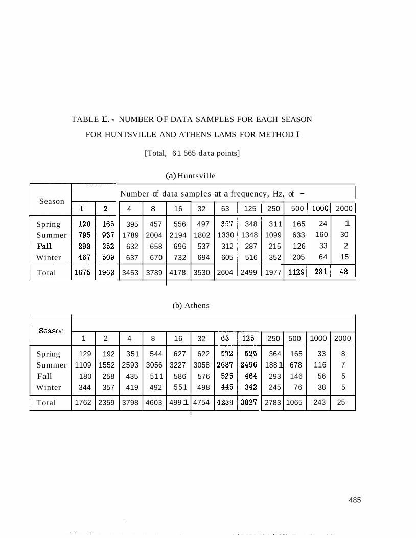
TABLE II.- NUMBER OF DATA SAMPLES FOR EACH SEASON
165 633 126 205
FOR HUNTSVILLE AND ATHENS LAMS FOR METHOD I
[Total, 61 565 data points]
24 1 160 30
33 2 64 15
(a) Huntsville
1
129 1109
180 344
1762
2 4
192 351 1552 2593 258 435 357 419
2359 3798
500
165 678 146 76
1065
1000 2000
33 8 116 7 56 5 38 5
243 25
Number of data samples at a frequency, Hz, of - I Season
Spring Summer
Winter
Total
63 I 125 I 250 16 500 I 10001 2000 32 4
395 1789
632 637
8
457 2004
658 670
3789
359 348 311 1330 1348 1099 312 287 215 605 ~ 516 1 352
2604 2499 1977
497 1802 537 694
3530
556 2 194
696 732
4178 3453
(b) Athens
I 250 8
544 3056
5 1 1 492
4603
32
622 3058
576 498
4754
16
627 3227
586 5 5 1
499 1
364 188 1 293 245
2783
Spring Summer Fall Winter
I Total
485

4 86
MICROPHONE LAYOUT FOR LAMS LINES
* . ATHENS LAMS
.. .'-' HUNTSVILLE LAMS .. . .. .. TYPICAL MICROPHONE
F-1 '.'. 2 e SOUND SOURCE
s-I2@@:s-,e 0 5
KILOMETERS SCALE 1:250.000
w 0 5 IO 15 20 25 30 35 0 5 IO 15 20
RANGE. KI LOM ETERS RANGE,KILOMETERS
Figure 1
VARIATIONS OF METHODS
METHOD I ALL POSSIBLE COMBINATIONS OF MICROPHONES
MICROPHONE9 Q 9 Q Q
METHOD II: COMPARISON WITH REFERENCE MICROPHONE
REFERENCE
PPPPPPP MICROPHONE
'I COMPARISON J2 J3 j4 l5 16
ORDER
METHOD TE PIECEWISE COMPARISONS OVER ENTIRE MEASUREMENT RANGE
PPPPPP UUUUUL
Figure 2

EXCESS ATTENUATION (METHOD I) FOR GROUND -TO- GROUND PROPAGATION FOR FALL SEASON AT MSFC,ALA.
.4 ATHENS LAMS A
EXCESS GROUND
0 I , I t ' I I , I
2 10 100 1000 OCTAVE BAND CENTER FREQ, Hz(cps)
Figure 3
ATTENUATION ( METHOD I) FOR GROUND -TO- PROPAGATION FOR SUMMER SEASON AT MSFC ,ALA.
1 .o c HUNTSVILLE LAMS
ATHENS LAMS
I I I I , I
2 10 100 1000 OCTAVE BAND CENTER FREQ , Hz(cps) . .
Figure 4
487
J
EXCESS ATTENUATION ( METHOD I) FOR GROUND -TO - GROUND PROPAGATION FOR WINTER SEASON AT MSFC,ALA.
0 0
\
U
:e m
8 I , I 3 I I I ,
2 10 100 1000 OCTAVE BAND CENTER FREQ, Hz(cps)
Figure 5
EXCESS ATTENUATION (METHOD I) FOR GROUND - T O - GROUND PROPAGATION FOR SPRING SEASON AT MSFC,ALA.
1.0
. 8 I-' LL
\
-0 m .4
I I I I I I l l I I I l l 2 10 100 1000
OCTAVE BAND CENTER FREQ , HdcPs)
Figure 6
488
a

EXCESS ATTENUATION FOR VARIOUS SEASONS METHOD I
, , I , I , I I ,
oh IO 100 1000 OCTAVE BAND CENTER FREQUENCY Hz (cps)
Figure 7
AVERAGE EXCESS ATTENUATION FOR ALL SEASOEJS 1.4 r METHOD I
1.2 -
1.0 -
.a -
dB/1000 ft
.2 -
I I I l l I I I l l I I I l l
1000 0 io 100 OCTAVE BAND CENTER FREQ, Hzkps)
Figure 8
4 89

EXCESS ATTENUATION FOR GROUND -TO-GROUND PROPAGATION
METHOD II ft, THOUSANDS
/ 8x10³ 3-01 5 / EA,
dB/1000 ft
2.0 -
2 IO IO0
18x103
36-58x103 -
d IO00
OCTAVE BAND CENTER FREQUENCY, Hz (cps)
Figure 9
VARIATION OF EXCESS ATTENUATION (dB/lOOOft) FOR GROUND-TO-GROUND PROPAGATION (METHOD II) FOR
VARIOUS DISTANCE WITH OCTAVE- BAND CENTER FREQUENCY (SUMMER SEASON-H U NTSVl LLE LAMS)
THOUSANDSOFFEET A'-
, , , I I I I l a ,
O h ' ' " " I ' IO I O 0 1000 OCTAVE BAND CENTER FREQUENCY, Hz. (cps)
Figure 10
490
EXCESS ATTENUATION (dB/IOOOft) AT A 2-KILOMETER DISTANCE AS A FUNCTION OF OCTAVE-BAND CENTER FREQUENCY,Hz
6.0[ 5.0 REF 5
(DNEPROVSKAYA) I
PRESENT ! , REF9
I I I 100 1000 IO 000
OCTAVE-BAN D CENTER FREQUENCY, HZ (CPS)
Figure 11
TYPICAL EXCESS ATTENUATION METHODS II AND m; 500 Hz CENTER
FREQUENCY BAND
2.0
'- METHOD IT
0 8 16 24 32 40 GROUND DIST., K FEET
Figure 12
491
49 2
EXCESS ATTENUATION FROM METHODS TIANDm (SUMMER SEASON)
250 Hz CENTER FREQUENCY BAND
1.6 - -
EA, 1.2 dB/1000ft -
.8 -
-
-
.4 -
0 8 16 24 32 40 48x103 DISTANCE, f t
Figure 13