2d unsteady computations for cosdyna > tony gardner > 21.06.2006 folie 1 2d unsteady...

Folie 12D unsteady computations for COSDYNA > Tony Gardner > 21.06.2006

2D unsteady computations with deformation and adaptation for COSDYNA

Tony Gardner

DLR AS-HK

2D unsteady computations for COSDYNA > Tony Gardner > 21.06.2006

Folie 2

Summary

Overview of project COSDYNA

Computational geometry

TAU deformation module

Adaptation scheme

Example computations and initial results

Conclusion


Folie 3

Show Video 1 (Example of method)


Folie 4

HighPerFlex

DLR internal High Performance Flexible Aircraft project (HighPerFlex) 2003-2006

LAWIA – (Last- und Widerstandsabminderung)

Load and drag reduction on a full A340 model by the steady CFD investigation of TED settings on an aeroelastically coupled aircraft.

COSDYNA – (Control surface dynamics)

Numerical and experimental investigation of unsteady profile and TED oscillations

JENIFA – (Jet engine interference in flutter analysis)

Experimental and numerical work to compliment the DLR-ONERA project WIONA (wing with oscillating nacelle)


Folie 5

COSDYNA unsteady computations

To compute unsteady coefficients for comparison with TWG experiments in October 2006

TWG experiments will be performed with a 2D VC-Opt airfoil in the adaptive test section. Forced oscillations of flap and airfoil can be programmed or the airfoil can swing freely.

Computations must be at least partially performed beforehand due to time constraints.

Computations must include flap and airfoil movement.

Optimally, computations will not include gap flow

Computations include cases with strong shocks, and thus will optimally allow adaptation


Folie 6

2D VC-Opt airfoil in TWG


Folie 7

Geometry

VC-Opt, length 300mm

Design Mach =0.775

With 25% flap (gapless) deployed by grid deformation

Re=2 million

2D CENTAUR grid

Farfield at r=50 chords

(needs farfield vortex correction)

Surface points at 2mm spacing

28 structured sublayers (no cell chopping)

Built for y+=1

Raw grid has 50,000 points before 2D reduction


Folie 8

Flap movement

Chimera

Requires a gap between body and flap (non-physical)

Gapless using automatic hole cutting is in development

Deformation

Can perform gapless movement

Requires definition of the new surface position

Handling the hinge requires care

Simplifies grid generation


Folie 9

TAU Deformation

Tau deformation takes a surface deformation and deforms the volume grid to enclose this new surface

The grid points and numbering (GID) are preserved in the new grid, changing only the grid point positions. Solutions in TAU use GID.

A deformation can be expressed as (x, y, z), (x, y, z) or as a 3D, algebraic test deformation (z=C{y-y0}2)

TAU version 2005.1.1

Not explicitly 2D (accumulated machine precision errors)

Adaptation level information destroyed on reading of grid

No 2D algebraic test deformation

TAU version 2006.1.0

Grid quality problems with incremental deformations

No 2D algebraic test deformation


Folie 10

TAU version

Based on 2005.1.1 with 2D adaptation patch

Added 2D deformation (Gerhold)

Added adaptation level loading (Gerhold)

Added 2D linear algebraic deformation

Deforming as: z=C(x-x0)

Using shell script in serial

Python was attempted, but I couldn’t get the scripts working.

Due to development status and lack of documentation?

Writing a solution each time step means that saved IO in Python is not as significant as it might be in other cases.


Folie 11

Script execution in serial (Data passing as disk write)

Adaptation

Unsteady solver

Deformation

Unsteady solver

Steady solver

Deformation

Adaptation

Steady solver

Steady starting solution (20 mins)

Unsteady computation (2-3 days)


Folie 12

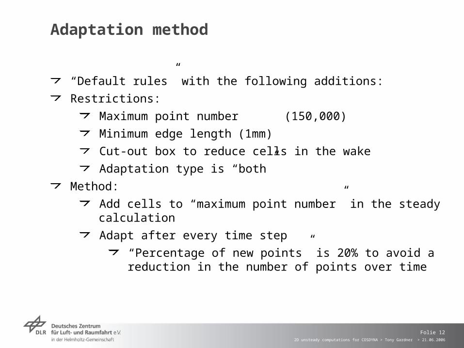
Adaptation method

“Default rules” with the following additions:

Restrictions:

Maximum point number (150,000)

Minimum edge length (1mm)

Cut-out box to reduce cells in the wake

Adaptation type is “both”

Method:

Add cells to “maximum point number” in the steady calculation

Adapt after every time step

“Percentage of new points” is 20% to avoid a reduction in the number of points over time


Folie 13

Example Grid 1/4


Folie 14

Example Grid 2/4


Folie 15

Example Grid 3/4


Folie 16

Example Grid 4/4


Folie 17

Time stepping study

Flap movement (): 0.0 1.0 degrees

Pitching amplitude (): 0.0 0.2 degrees

Reduced frequency (): 0.40 / 0.80

Ma: 0.80

Steps/period: 25, 50, 100, 200


Folie 18


Folie 19

Grid refinement study

Very difficult to undertake, even in 2D

Currently testing against a number of static, unrefined grids

Problems with large grid sizes of static grids

Refinement cases where surface grid size and tetrahedral stretching were reduced did not converge, up to 300000 cells.

Currently trying other refinement methods.


Folie 20


Folie 21


Folie 22

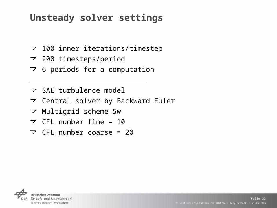
Unsteady solver settings

100 inner iterations/timestep

200 timesteps/period

6 periods for a computation

SAE turbulence model

Central solver by Backward Euler

Multigrid scheme 5w

CFL number fine = 10

CFL number coarse = 20


Folie 23

Show Videos 2 and 3

Ma=0.8

Re=2 million

=0.15 (~20 Hz)

Video2: Body oscillation only. = 0.0 0.2 degrees

Video3: Flap oscillation only. = 0.0 1.0 degrees


Folie 24

First results


Folie 25

Conclusions and further work

Under special conditions, 2D unsteady computations with adaptation and deformation appear to work.

Verification of the results with experiment still needs to be undertaken.

Grid refinement studies are still a problem

A similar approach could be undertaken using Python scripting.

2d unsteady computations for cosdyna > tony gardner > 21.06.2006 folie 1 2d unsteady...

Documents