26 april 2013lecture 6: problem solving1 problem solving jorge cruz di/fct/unl april 2013
Post on 22-Dec-2015
216 views
TRANSCRIPT
26 April 2013 Lecture 6: Problem Solving 1
Problem Solving
Jorge CruzDI/FCT/UNL
April 2013
Lecture 6: Problem Solving 2
Problem Solving
Variable Elimination
Dependency Reduction
Modelling Techniques
System Scaling
Constraint Solving Systems
Interval Libraries
Some Languages and Tools
Some Common Benchmarks
Some Problems
26 April 2013
Final Project
Lecture 6: Problem Solving 3
Modelling Techniques
Frequently a single problem may be modelled by several equivalent CCSPs
The behaviour of a constraint solver may change drastically even with equivalent CCSPs
To choose the best model for a particular problem is important to understand the underlying constraint propagation algorithms
Some modelling techniques are commonly adopted for improving the accuracy and efficiency of the continuous constraint solvers
26 April 2013

Lecture 6: Problem Solving 4
Modelling Techniques
A fundamental problem of interval arithmetic is the dependency problem (see lecture 2).
Dependency Reduction
Dependency Problem. In the interval arithmetic evaluation of an interval expression, each occurrence of the same variable is treated as a different variable. The dependency between the different occurrences of a variable in an expression is lost.
Some expressions may be rewritten into equivalents that minimize the dependency problem
Factorize as much as possible polynomial expressions:Instead of using constraint x2y2+xy2+xy=0 use constraint xy(y(x+1)+1)=0
Use better interval extensions (mean value form, Taylor form,…):Instead of using constraint xx2=0 use constraint 0.25(x0.5)2=0
Examples:
26 April 2013

Lecture 6: Problem Solving 5
Modelling Techniques
Precision and efficiency may be improved if the number of variables is reduced
Variable Elimination
Sometimes a set of constraints may be rewritten into an equivalent set with less variables
Example:
Continuous constraint solvers rely on the efficiency of branch and prune algorithms for enforcing consistency on the CCSP variables
Instead of using the constraint system:
x1 + x2 + x3 = 1(x1 + x1x2 + x2x3) x4= c1
(x2 + x1x3) x4= c2
x3x4 = c3
Consider x4 = c3/x3 and use the constraint system:x1 + x2 + x3 = 1(x1 + x1x2 + x2x3)c3 = c1x3
(x2 + x1x3)c3 = c2x326 April 2013

Lecture 6: Problem Solving 6
Modelling Techniques
A consequence of numerical errors is the amplification of the variable domains and poor pruning results
System Scaling
Two major sources of numerical errors are:operations with large numbers (lower density of F-Numbers at this ranges)operands with different magnitudes
Scaling the system and making some variable substitutions may avoid such situations as much as possible
Continuous constraint solvers rely on interval techniques for dealing with numerical errors.
Consider x = 1020y and use the constraint: y2+3y+2=0
Example:
Instead of using constraint: 10-20x2+3x+2×1020=0
26 April 2013
Lecture 6: Problem Solving 7
Some Languages and Tools
PROFIL/BIAS (Programmer's Runtime Optimized Fast Interval Library) http://www.ti3.tu-harburg.de/Software/PROFILEnglisch.html
Interval Libraries
GAOL: NOT Just Another Interval Library
http://sourceforge.net/projects/gaol
smath (routines for interval arithmetic and constraint narrowing)
http://interval.sourceforge.net/interval/prolog/clip/clip/smath/README.html
CFILIB (Fast Interval LIBrary)
http://www.math.uni-wuppertal.de/org/WRST/software/filib.html
FILIB++ (Fast Interval LIBrary in C++)
http://www.math.uni-wuppertal.de/org/WRST/software/filib.html
C++
26 April 2013
Lecture 6: Problem Solving 8
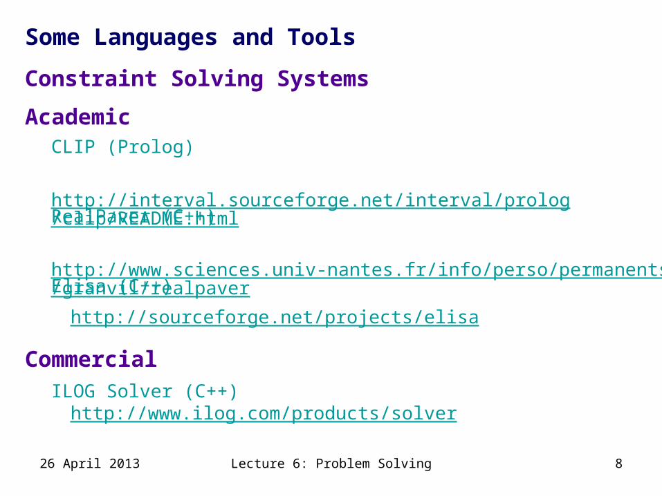
Some Languages and Tools
ILOG Solver (C++)http://www.ilog.com/products/solver
Constraint Solving Systems
Elisa (C++)
http://sourceforge.net/projects/elisa
RealPaver (C++)
http://www.sciences.univ-nantes.fr/info/perso/permanents/granvil/realpaver
AcademicCLIP (Prolog)
http://interval.sourceforge.net/interval/prolog/clip/README.html
Commercial
26 April 2013
Lecture 6: Problem Solving 9
Some Problems
Many continuous problems may be modelled and solved as CCSPs.
Some Common Benchmarks
Several benchmarks are commonly used to address the quality of the constraint solvers.
The following problems illustrate some common benchmarks in interval constraints.
For each benchmark we would like to know where are the solutions (if any) satisfying the constraints within the specified ranges
26 April 2013

Lecture 6: Problem Solving 10
Some Problems
2x1=2 2x2=1 2x3=2 2x4=1 2x5=x6
x5+2x6=2 (x1-x7)2+x8
2-x72=(x8-x2)2
(x1-x7)2+x82-(x3-x7)2=(x4-x8)2
x12+x2
2-2x1x7+2x2x8=0 x1
2-x33-x4
2-2x7(x1-x3)+2x4x8=0
Appolonius
Ranges:
Constraints:
x1, x2, x3, x4, x5, x6, x7, x8[-108,108]
26 April 2013

Lecture 6: Problem Solving 11
Some Problems
x2 + y2 + z2 = 36x + y = zxy + z2 = 1
Bronstein
Ranges:
Constraints:
x, y, z[-108,108]
26 April 2013
Lecture 6: Problem Solving 12
Some Problems
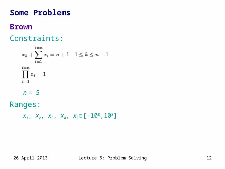
Brown
Ranges:
Constraints:
n = 5
x1, x2, x3, x4, x5[-108,108]
26 April 2013
Lecture 6: Problem Solving 13
Some Problems
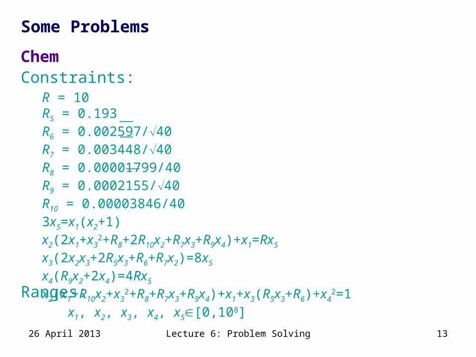
R = 10 R5 = 0.193 R6 = 0.002597/40 R7 = 0.003448/40 R8 = 0.00001799/40 R9 = 0.0002155/40 R10 = 0.00003846/40 3x5=x1(x2+1) x2(2x1+x3
2+R8+2R10x2+R7x3+R9x4)+x1=Rx5
x3(2x2x3+2R5x3+R6+R7x2)=8x5
x4(R9x2+2x4)=4Rx5
x2(x1+R10x2+x32+R8+R7x3+R9x4)+x1+x3(R5x3+R6)+x4
2=1
Chem
Ranges:
Constraints:
x1, x2, x3, x4, x5[0,108]
26 April 2013
Lecture 6: Problem Solving 14
Some Problems
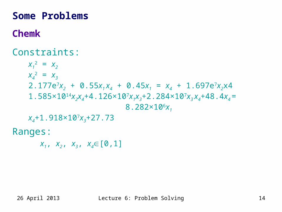
x12 = x2
x42 = x3
2.177e7x2 + 0.55x1 x4 + 0.45x1 = x4 + 1.697e7x2x41.585×1014x2x4+4.126×107x1x3+2.284×107x3 x4+48.4x4 =
8.282×106x1 x4+1.918×107x3+27.73
Chemk
Ranges:
Constraints:
x1, x2, x3, x4[0,1]
26 April 2013

Lecture 6: Problem Solving 15
Some Problems
y2z2 + y2 + z2 + 13 = 24yzx2z2 + x2 + z2 + 13 = 24xzx2y2 + x2 + y2 + 13 = 24xy
Cyclo
Ranges:
Constraints:
x, y, z[0,105]
26 April 2013
Lecture 6: Problem Solving 16
Some Problems
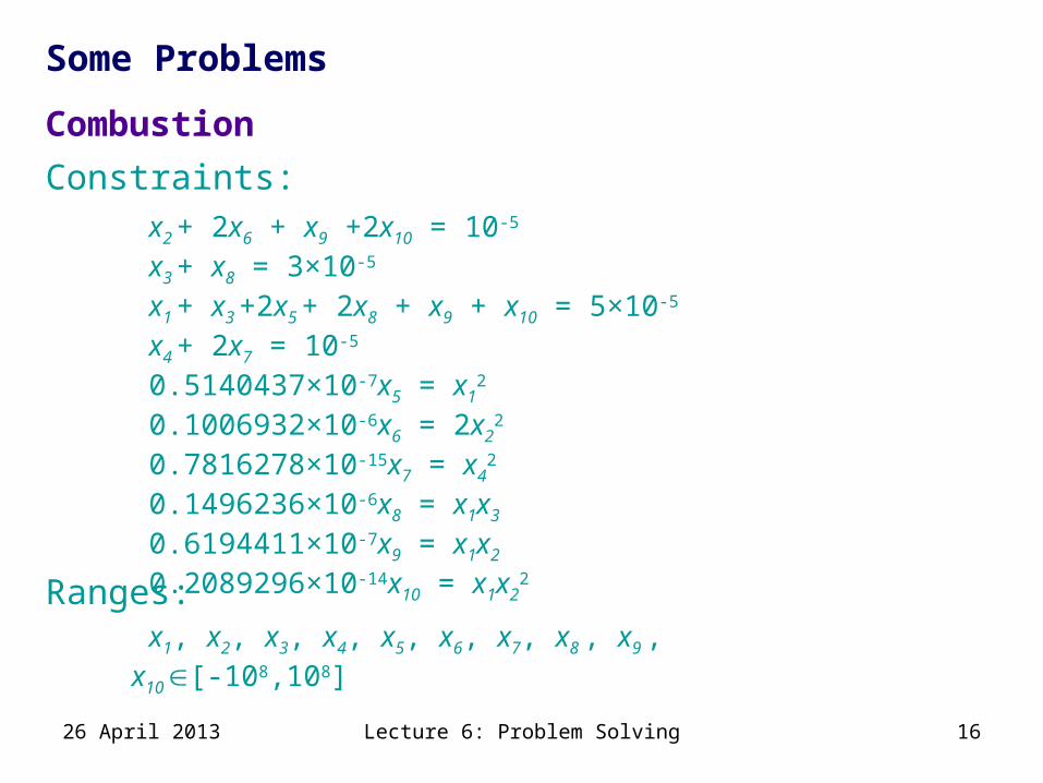
x2 + 2x6 + x9 +2x10 = 10-5
x3 + x8 = 3×10-5
x1 + x3 +2x5 + 2x8 + x9 + x10 = 5×10-5
x4 + 2x7 = 10-5
0.5140437×10-7x5 = x12
0.1006932×10-6x6 = 2x22
0.7816278×10-15x7 = x42
0.1496236×10-6x8 = x1x3
0.6194411×10-7x9 = x1x2
0.2089296×10-14x10 = x1x22
Combustion
Ranges:
Constraints:
x1, x2, x3, x4, x5, x6, x7, x8 , x9 , x10 [-108,108]
26 April 2013

Lecture 6: Problem Solving 17
Some Problems
x1 +5x22 = x2
3 + 2x2 + 13x1 + x2
3 + x22
= 14x2 + 29
Freudenstein
Ranges:
Constraints:
x1, x2[-108,108]
26 April 2013
Lecture 6: Problem Solving 18
Some Problems
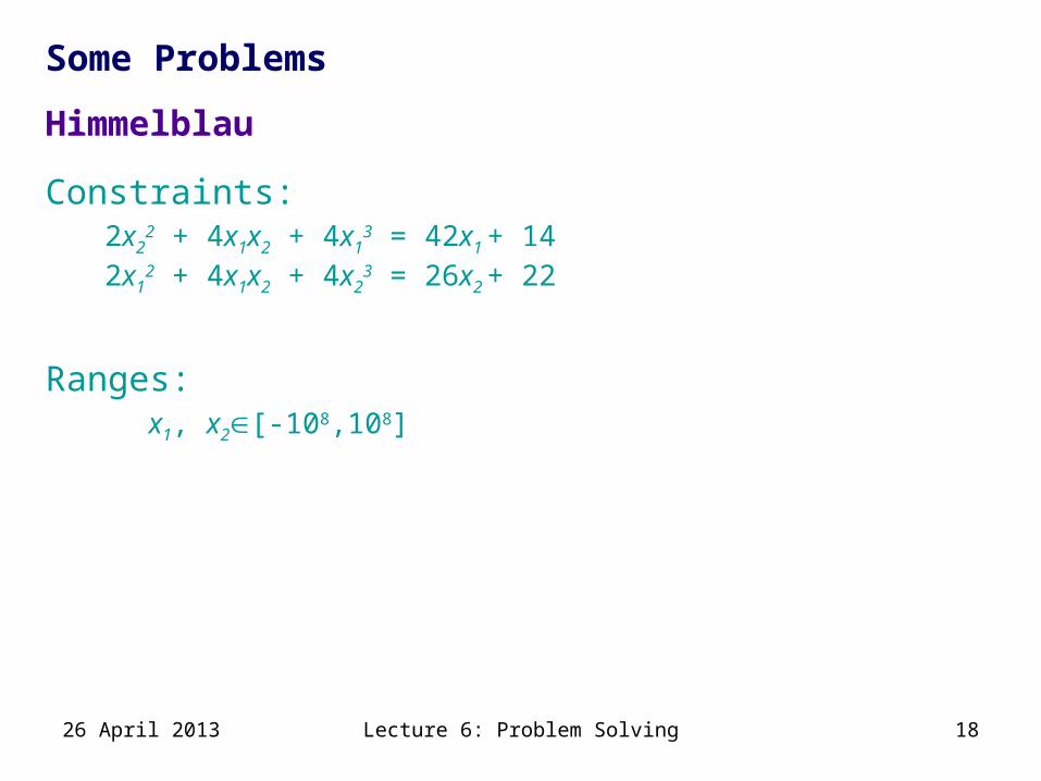
2x22 + 4x1x2 + 4x1
3 = 42x1 + 142x1
2 + 4x1x2 + 4x23 = 26x2 + 22
Himmelblau
Ranges:
Constraints:
x1, x2[-108,108]
26 April 2013
Lecture 6: Problem Solving 19
Some Problems
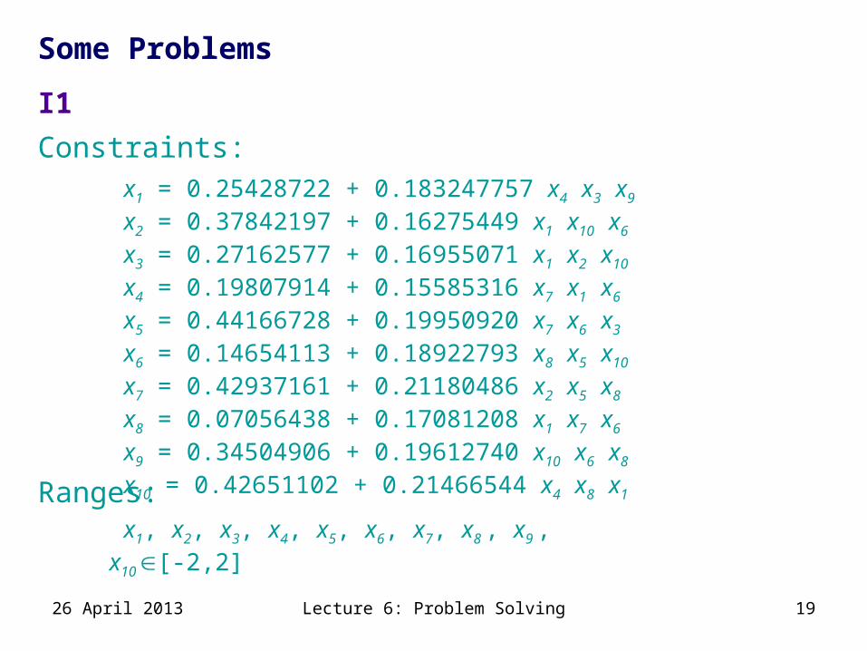
x1 = 0.25428722 + 0.183247757 x4 x3 x9 x2 = 0.37842197 + 0.16275449 x1 x10 x6 x3 = 0.27162577 + 0.16955071 x1 x2 x10 x4 = 0.19807914 + 0.15585316 x7 x1 x6 x5 = 0.44166728 + 0.19950920 x7 x6 x3 x6 = 0.14654113 + 0.18922793 x8 x5 x10 x7 = 0.42937161 + 0.21180486 x2 x5 x8 x8 = 0.07056438 + 0.17081208 x1 x7 x6 x9 = 0.34504906 + 0.19612740 x10 x6 x8 x10 = 0.42651102 + 0.21466544 x4 x8 x1
I1
Ranges:
Constraints:
x1, x2, x3, x4, x5, x6, x7, x8 , x9 , x10 [-2,2]
26 April 2013

Lecture 6: Problem Solving 20
Some Problems
6(x1 x2 - x3 x4) + 10 x1 = 1 6(x1 x4 + x2 x3) + 10 x3 = 4 x1
2 + x32 = 1
x22 + x4
2 = 1
Kincox
Ranges:
Constraints:
x1, x2, x3, x4 [-1,1]
26 April 2013
Lecture 6: Problem Solving 21
Some Problems
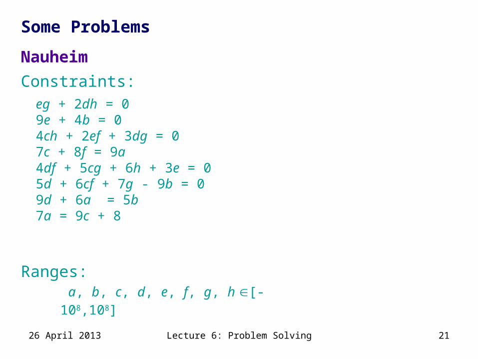
eg + 2dh = 09e + 4b = 04ch + 2ef + 3dg = 07c + 8f = 9a4df + 5cg + 6h + 3e = 05d + 6cf + 7g - 9b = 09d + 6a = 5b7a = 9c + 8
Nauheim
Ranges:
Constraints:
a, b, c, d, e, f, g, h [-108,108]
26 April 2013
Lecture 6: Problem Solving 22
Some Problems
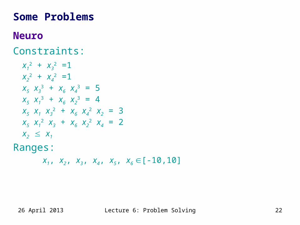
x12 + x3
2 =1x2
2 + x42 =1
x5 x33 + x6 x4
3 = 5x5 x1
3 + x6 x23 = 4
x5 x1 x32 + x6 x4
2 x2 = 3x5 x1
2 x3 + x6 x22 x4 = 2
x2 x1
Neuro
Ranges:
Constraints:
x1, x2, x3, x4, x5, x6 [-10,10]
26 April 2013
Lecture 6: Problem Solving 23
Some Problems
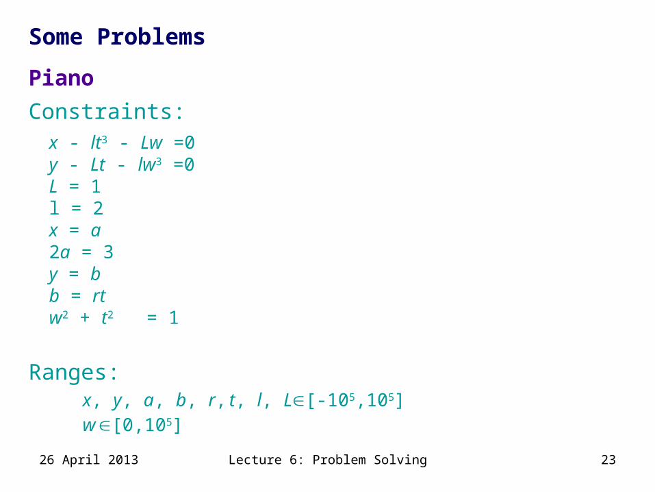
x - lt3 - Lw =0y - Lt - lw3 =0L = 1 l = 2x = a2a = 3y = bb = rtw2 + t2 = 1
Piano
Ranges:
Constraints:
x, y, a, b, r, t, l, L[-105,105] w [0,105]
26 April 2013

Lecture 6: Problem Solving 24
Some Problems
x12 + x2
2 =1x3
2 + x42 =1
x52 + x6
2 =1x7
2 + x82 =1
0.004731x1x3 + x7 = 0.3578x2x3 + 0.1238x1 + 0.001637x2 + 0.9338x4 + 0.35710.2238x1x3 + 0.7623x2x3 + 0.2638x1 = 0.07745x2 + 0.6734x4 + 0.6022 + x7
x6 x8 + 0.3578x1 + 0.004731x2 = 00.2238x2 + 0.3461 = 0.7623x1
Robot Kinematics
Ranges:
Constraints:
x1, x2, x3, x4, x5, x6, x7, x8 [-1,1]
26 April 2013

Lecture 6: Problem Solving 25
Project
Use interval constraint techniques to solve systems of nonlinear equations that models Social Argumentation Networks [1].
The problem
These are systems with n equations and n unknowns of the form:
with 1in, xi[0,1], ai(0,1) and mji{0,1}
[1] J. Leite and J. Martins. Social abstract argumentation. In Proceedings of IJCAI'11, volume 3, 2011.
26 April 2013
n
jjjiii xmax
1
)1(

Lecture 6: Problem Solving 26
Project
Solve the following systems:a)
b)
c)
Task 1
26 April 2013
)1(8.0)1(2.0
)1)(1(86.0)1)(1(5.0
)1(5.0
45
54
543
312
21
xxxx
xxxxxx
xx
)1)(1(9.0)1)(1(9.0)1)(1(9.0
323
212
311
xxxxxxxxx
)1)(1(8.0)1)(1(7.0)1)(1(9.0
213
312
321
xxxxxxxxx
Lecture 6: Problem Solving 27
Project
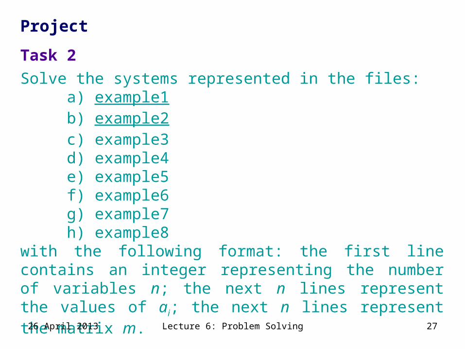
Solve the systems represented in the files: a) example1b) example2c) example3d) example4e) example5f) example6g) example7h) example8
with the following format: the first line contains an integer representing the number of variables n; the next n lines represent the values of ai; the next n lines represent the matrix m.
Task 2
26 April 2013

Lecture 6: Problem Solving 28
Project
a) Implement na application to generate and solve a random system of n variables.
b) Solve random systems of 5, 10, 15, 20, 25, … variables (10 instances of each) and produce a table with statistical information of its performance (execution time, number of splits, …)
Task 3
26 April 2013