problem statement problem solution
TRANSCRIPT

16.851 Assignment #1, 2003-09-17
Problem Statement
Motivation The design of a spacecraft power subsystem is an important driver for the mass, size, and capability of the spacecraft. Every other spacecraft subsystem is affected by the power subsystem, and in particular, important issues such as communications bandwidth, thermal regulation, and structural design are largely influenced by the capabilities and limitations of the power system. The motivation for this problem is the broad applicability of a power-system design tool to a wide range of future design problems.
Requirements Given time histories of the power load and power source, design a power subsystem that optimizes with respect to some specified cost function. The power source profile can be specified directly, or determined from constituent information such as time histories of the sunlight intensity and the changing angle of a solar panel as a spacecraft rotates with respect to the sun. The design space for the power subsystem should contain several types of power generation devices, such as photovoltaic arrays and radioisotope thermoelectric generators; and several types of energy storage devices, such as batteries and flywheels. From this design space, a system that minimizes the cost function should be selected.
Problem Solution The approach taken to the problem is to create a set of modular functions that are combined to achieve a solution. The primary advantage to using this approach is that small, simple blocks of code can be validated more easily than large, complex blocks.
Inputs Required user inputs include the following quantities:
- Load power as a function of time in Watts, sampled at constant time steps. - Source power as a function of time in Watts, sample at constant time steps. This can
be supplied either directly as a power profile, or indirectly as constituent data such as the time histories of incident sunlight intensity and angle of solar array with respect to the sun.
- The length of the time step in seconds. - The initial life fraction of the energy storage device. - The energy initially stored in the energy storage device, in Joules.
Outputs Outputs from the design module include the following quantities:
- The mass of the power system in kilograms, including the mass of the energy storage system (batteries or flywheel) and power generation system (solar array or RTGs). This mass does not include other components of the system such as power conditioning electronics.

- The cost of the energy storage and power generation systems in millions of dollars. - The time history of the state of charge of the energy storage system, in Joules. - The time indices at which the energy storage capacity was insufficient to meet
demand, if this has occurred. - The time history of excess thermal energy that must be dissipated, in Joules. - The remaining life in the storage system as a fraction of the original lifespan.
Formulas and Constraint Equations When determining the state of charge for an energy storage device, two constraint equations must be satisfied at all times. First, the integral of the load power must be less than the sum of the integral of the source power and the initial stored energy, as shown in the following equation.
t t ( )Pload dτ ≤ ∫ P dτ + t E 0source t0
∫t0
Secondly, because it is impossible for an energy storage device to contain negative energy, the energy contained in the device is constrained by a lower bound at zero, and by an upper bound at the device maximum capacity Emax.
Emax ( )≥ 0≥ t E
The fraction of the lifetime lost due to a particular discharge/charge cycle on a chemical battery can be determined using the following formula, where ∆Li is the fraction lost, di is the depth of discharge, b is the intercept, and m is the slope. This equation was derived from Fig. 11-11 in SMAD.
⎛ di −b ⎞−⎜ ⎟ ⎝ m ⎠∆Li = −10
The remaining lifetime fraction as a function of time can then be determined by summing the fractions lost due to each cycle. In the following equation, the lifetime fraction is L0
at time t0. n
(t L − t0 )= L + ∑∆Lin 0 i =0
These equations summarize many of the major interactions between elements of the power subsystem.
Files The following files, listed in alphabetical order, are used in the calculation of the optimal power system and the validation of components of the power system model. The main function is masterloop.m; all of the other functions, with the exception of the validation functions, are called from within the function masterloop. A simplified flow diagram for the module is shown in Figure 1.

= =
×
yes yes
no no
masterloop.m
PowerDesignResult.m
Design Vector
Power Source
Solar Array
Power Source
RTG
SolarArrayPerArea.m
Surface Area
RTGPower.m
battery_profile.m
error
Design Vector
Figure 1. Simplified flow diagram.
battery_profile.m - Calculates the time profiles of the energy storage device state of charge and excess
thermal energy. Determines if the power and energy devices are sufficient to handle the applied load.
- Calculates the cumulative effect of individual discharge/charge cycles on the device lifetime.
- Inputs include the properties of the energy storage device and the time histories of the source and load power.
- This file contains the functions battery_profile and delta_life. - Validated using MER_sol4.m.
EffectivePowerIntensity.m - Used to compute the effective solar radiation intensity based on the incident angle
between the line of radiation and a vector normal to the solar array surface.

- As the incident angle is a function of time, the resulting effective power intensity is also a function of time.
masterloop.m - The main function, from which the other functions are called. Operates with a set of
nested ‘for’ loops, which are used to test all possible combinations of designs.
MER_sol4.m - Used to validate the model used in battery_profile.m. This function can be
run from the command line without any additional inputs. - Reads in the source (solar array) and load (egress operations) power profiles for the
Mars Exploration Rover egress scenario planned for sol 4, as reported in the MER Mission Plan.
- Uses battery_profiles.m to recreate the battery state of charge history shown in the MER Mission Plan, and plots the recreated profile against the MER Missoin Plan profile.
- Requires the Excel spreadsheet MER_sol4_input_data.xls. The accuracy of the input data is limited by the fact that the data points were eyeballed from the plot in the mission plan and copied to Excel point by point.
- This file contains the functions MER_sol4, plot_results, corner_times, create_profile, and t2m.
MER_sol4_input_data.xls - A spreadsheet containing data points from MER_sol4_power_profile.png.
Used for validation of the function battery_profile.
MER_sol4_power_profile.png - A bitmap screen capture of the energy balance plot for MER A sol 4 egress
operations, taken from the MER Mission Plan. Used for validation of the function battery_profile.
plot_battery_dod_cycles.m - Used to visualize the effect of a single discharge/charge cycle on the lifetime of a
battery. Creates a plot of depth of discharge as a function of fraction of lifetime lost for all types of chemical batteries being considered. This function can be run from the command line without any additional inputs.
PowerDesignResult.m - Given the design requirements and the specification of the power source and energy
storage devices, PowerDesignResult.m computes the overall mass and cost, the power available from the power source as a function of time, and the state of charge of the energy storage device as a function of time.
- The function may also return a set of time instances at which the stored energy was insufficient to handle the power load. Furthermore, it computes the energy storage device’s remaining life and required energy dissipation.

- Depends on SolarPowerPerArea.m and battery_profile.m to compute the aforementioned information.
power_read_xls.m - Reads in an Excel spreadsheet containing data on power generation and energy
storage devices (e.g. RTGs, photovoltaics, batteries, fly-wheels, etc.), and saves the information to Matlab structures.
RTGPower.m - Used to compute the power an RTG can generate. The power an RTG can generate
depends on the specific model of the RTG.
slope_intercept.m - Given a particular set of energy storage device properties, calculates the slope and
intercept of the plot of depth of discharge as a function of cycle life. The slope is considered constant, based on the limited data available from SMAD and external sources.
SolarPowerPerArea.m - Used to determine the amount of power that can be generated from a unit area of a
solar array, based on the type of the solar array and the effective illumination intensity. It takes into account the degradation of the array over the time period, the efficiency of the solar array, and the inherent degradation (i.e. degradation of the solar array system due to the temperature and shadowing effects) [SMAD].
- Depends on EffectivePowerIntensity.m for computing the effective power intensity.
TestPowerDesignResult.m - This function is used to validate the functionality of PowerDesignResult.m
through a simplified LEO scenario.
TestSolarArray.m - This function is used to validate the functionality of SolarPowerPerArea.m and EffectivePowerIntensity.m through a simplified LEO scenario.
Module Validation
Energy Storage for MER Several of the functions used in the module are validated individually. Among these is the battery_profile function, which is validated using data from the MER Mission Plan, as shown in Figure 2. The function MER_sol4.m reads the source and load power profiles from an Excel spreadsheet, parses the data, and passes the power profiles to battery_profile, which generates the Battery SOC and Excess Power profiles. The top plot is taken from the MER Mission Plan, the middle plot shows the inputs to and outputs from the function battery_profile, and the bottom plot shows these inputs
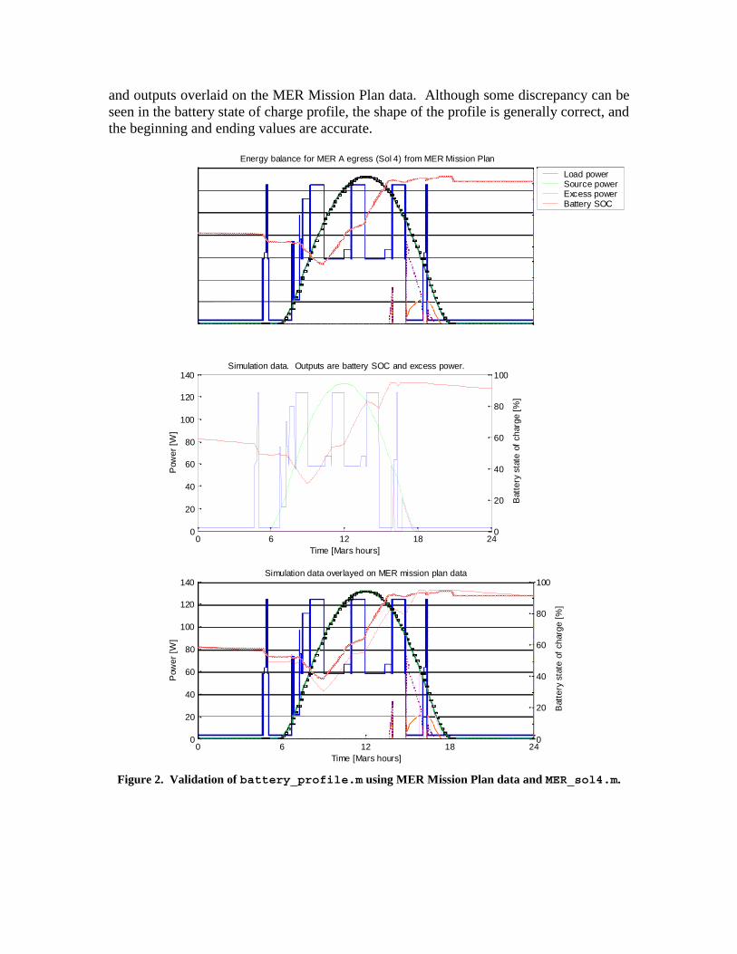
and outputs overlaid on the MER Mission Plan data. Although some discrepancy can be seen in the battery state of charge profile, the shape of the profile is generally correct, and the beginning and ending values are accurate.
Energy balance for MER A egress (Sol 4) from MER Mission Plan
Load power Source power Excess power Battery SOC
Pow
er [
W]
Simulation data. Outputs are battery SOC and excess power. 140 100
120 80
100
6080
60 40
40
20 20
Bat
tery
sta
te o
f ch
arge
[%
]
0 0 0 6 12 18 24
Time [Mars hours]
Simulation data overlayed on MER mission plan data
0
20
40
60
80[W]
0
20
40
60
80
]
100
120
140
Pow
er
100
Bat
tery
sta
te o
f ch
arge
[%
0 6 12 18 24 Time [Mars hours]
Figure 2. Validation of battery_profile.m using MER Mission Plan data and MER_sol4.m.

Depth of discharge and cycle lifetime The issue of battery lifetime dependence on depth of discharge and number of cycles is addressed by treating each discharge/charge cycle as an individual event, and tracking the cumulative effect of the individual events. Data in SMAD and elsewhere were used to create the relationships between depth of discharge and degradation of lifetime shown in Figure 3. The slopes of the lines are considered constant, based on data in SMAD. This figure may be plotted using plot_battery_dod_cycles.m.
Dep
th o
f di
scha
rge
[%]
Depth of discharge vs cycle life for secondary batteries 100
90
80
70
60
50
40
30
20
10
0
iSil i
Nickel-Hydrogen IPV (RNH30-9) Lith um Ion (INCP77)
ver Z nc (SZHR25) Nickel-Hydrogen CPV (RNHC4-1)
0 -1 -2 -3 -4 -5 -6 -7 -8 Fraction of life lost in one charge/discharge cycle [log10(x)]
Figure 3. Relationship between depth of discharge and reduction in lifetime for chemical batteries.
Solar Arrays The test function TestSolarArray.m is used to validate SolarPowerPerArea.m and EffectivePowerIntensity.m within a specific scenario. This scenario assumes a satellite in a low Earth circular orbit. The satellite has a fixed solar array, that is, the incident angle of the solar array with respect to the line of solar radiation varies in between -π and π. We also assume that the solar array is double sided and is never eclipsed by Earth. Figure 4 is the output generated by TestSolarArray.m.
Figure 4. Solar array power intensity for a simulated low Earth orbit without an eclipse.

The blue lines represent the solar radiation intensity, which is approximately 1367 W/m2. The green line is the effective radiation intensity the solar panels can absorb. Note that the effective solar radiation is periodic due to the periodicity of the incident angle. The red line represents the total power generated by the solar array. As shown by the plot on the left, this line tracks the effective solar radiation (green), but with lower magnitude due to the efficiency of the solar array. The plot on the right with larger time scale exhibits the degradation of the solar array as expected. Given a solar array, the power generated by the solar array is:
� (P = η ⋅ Id ⋅ Ieff ⋅ A ⋅ (1 − (D + t D − t0 )))0
where η is the efficiency, Id is the inherent degradation, Ieff is the effective radiation �intensity, A is the surface area exposed to the radiation, D0 is the initial degradation, D is
the rate of degradation, t is the current time, and t0 is the initial time. While the harsh environment (e.g. thermal cycling and micrometeoroid strikes) causes degradation/rate of degradation, the inherent degradation is caused by design inefficiencies (e.g. shadowing).
Radioisotope Thermoelectric Generators
The function RTGPower.m exhibits exponentially decaying power, as expected of a radioisotope thermoelectric generator.
Figure 5. RTG power vs. time.
We model the power generated by an RTG using an exponentially decaying function:
P = P0 ⋅ e−kt ,
where k is 1/87.74 [1/years] for Pu-238 that is typically used for an RTG.
Module Results The module was run using the input power profile and incident angle profile shown in Figure 6 and Figure 7, respectively. The profile was chosen to approximate a Low Earth Orbit to a very crude level. The fraction of life span remaining at the start of the period was chosen to be one, and a maximum energy storage capacity of 161280 J was chosen, a factor of ten less than the capacity of the Mars Exploration Rover batteries. The initial energy in the batteries was selected as 60% of this amount.
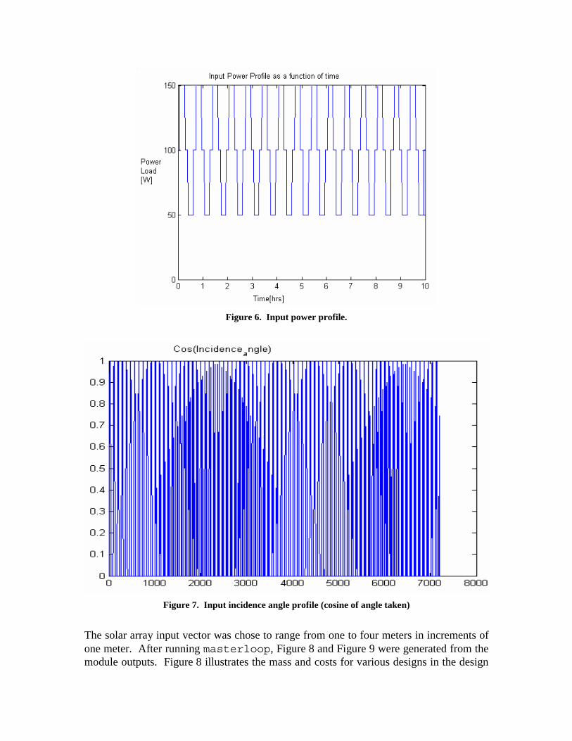
Figure 6. Input power profile.
Figure 7. Input incidence angle profile (cosine of angle taken)
The solar array input vector was chose to range from one to four meters in increments of one meter. After running masterloop, Figure 8 and Figure 9 were generated from the module outputs. Figure 8 illustrates the mass and costs for various designs in the design
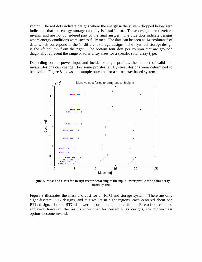
vector. The red dots indicate designs where the energy in the system dropped below zero, indicating that the energy storage capacity is insufficient. These designs are therefore invalid, and are not considered part of the final answer. The blue dots indicate designs where energy conditions were successfully met. The data can be seen as 14 “columns” of data, which correspond to the 14 different storage designs. The flywheel storage design is the 2nd column from the right. The bottom four dots per column that are grouped diagonally represent the range of solar array sizes for a specific solar array type.
Depending on the power input and incidence angle profiles, the number of valid and invalid designs can change. For some profiles, all flywheel designs were determined to be invalid. Figure 8 shows an example outcome for a solar-array based system.
Figure 8. Mass and Costs for Design vector according to the input Power profile for a solar array source system.
Figure 9 illustrates the mass and cost for an RTG and storage system. There are only eight discrete RTG designs, and this results in eight regions, each centered about one RTG design. If more RTG data were incorporated, a more distinct Pareto front could be achieved; however, the results show that for certain RTG designs, the higher-mass options become invalid.
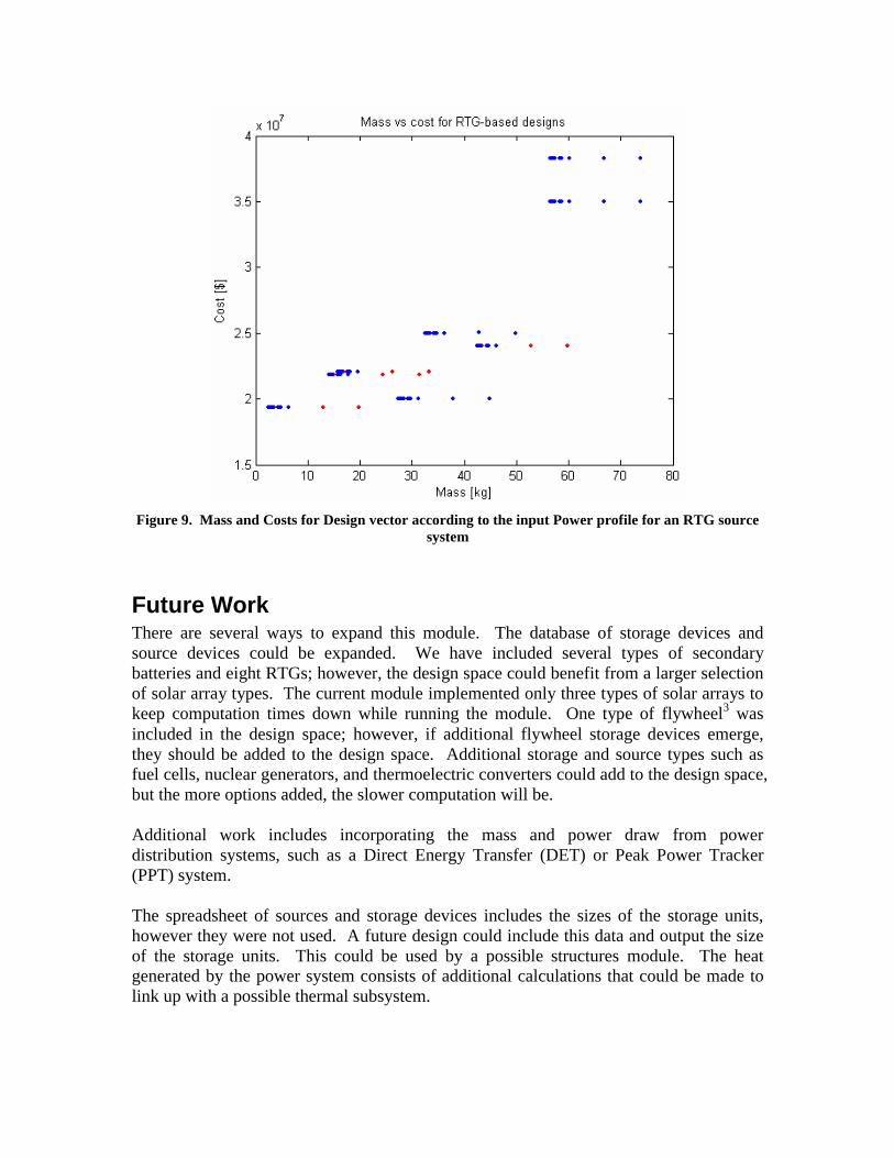
Figure 9. Mass and Costs for Design vector according to the input Power profile for an RTG source system
Future Work There are several ways to expand this module. The database of storage devices and source devices could be expanded. We have included several types of secondary batteries and eight RTGs; however, the design space could benefit from a larger selection of solar array types. The current module implemented only three types of solar arrays to keep computation times down while running the module. One type of flywheel3 was included in the design space; however, if additional flywheel storage devices emerge, they should be added to the design space. Additional storage and source types such as fuel cells, nuclear generators, and thermoelectric converters could add to the design space, but the more options added, the slower computation will be.
Additional work includes incorporating the mass and power draw from power distribution systems, such as a Direct Energy Transfer (DET) or Peak Power Tracker (PPT) system.
The spreadsheet of sources and storage devices includes the sizes of the storage units, however they were not used. A future design could include this data and output the size of the storage units. This could be used by a possible structures module. The heat generated by the power system consists of additional calculations that could be made to link up with a possible thermal subsystem.

Subsystems which would act as inputs to this power module include orbits, and environment. Environment already has an input, the form of the Solar Intensity, but additional data could be added. The Orbits subsystem has an effect on the Effective Intensity, and on the Power Input profile.
References 1. Wertz, J., and Larson, W., Space Mission Analysis and Design, Third Edition.
Torrance, CA: Microcosm Press, 1999. 2. Ludwinski, J., et. al., “Mars Exploration Rover (MER) Project Mission Plan,”
Pasadena, CA: Jet Propulsion Laboratory, April 24, 2002, JPL-D19659. 3. Designfax, http://www.manufacturingcenter.com/dfx/archives/0701/0701fly.asp,
Sept. 16, 2003. 4. Eagle-Picher, http://www.epcorp.com/EaglePicherInternet/, Sept. 16, 2003
Source Code Following are the full contents of the Matlab and Excel source code used in this assignment.
battery_profile.m function [energy,invalid,dissipation,life] = battery_profile(nsteps, dt, load, source, e_init, e_max, life_init, efficiency, slope, intercept) %[ENERGY, INVALID, DISSIPATION, LIFE] % = BATTERY_PROFILE(NSTEPS,DT,LOAD,SOURCE,E_INIT,E_MAX,LIFE_INIT,EFFICIENCY,SLOPE,INTERCEPT) % % Inputs: % NSTEPS The number of uniformly-spaced time values % DT [s] The separation between the time values % LOAD [W] The time profile of the power load % SOURCE [W] The time profile of the power source % E_INIT [J] The initial stored energy in the storage device % E_MAX [J] The capacity of the energy storage device % LIFE_INIT The fraction of the device’s usable life as of the start of the period % EFFICIENCY The fraction of the input energy that is recoverable % SLOPE The slope of the depth of discharge vs log life fraction plot % INTERCEPT The y-intercept of the depth of discharge vs log life fraction plot % % Outputs: % ENERGY [J] The time profile of the energy stored in the device % INVALID Indices of times at which the stored energy is negative (!) % DISSIPATION [W] The time profile of excess energy to be dissipated % LIFE The fraction of the device’s usable life as of the end of the period % % Note that if LENGTH(INVALID)>0, the capacity of the energy storage device is insufficient % to meet demand, and this is an invalid design. Any function calling BATTERY_PROFILE(...) % should verify that INVALID is empty before proceeding with further calculations. %
% reject any invalid inputs if (nsteps<2) error(’Error! NSTEPS must be at least two.’); end if (dt<=0) error(’Error! Time step DT must be greater than zero.’); end if (length(load) ~= nsteps) error(’Error! Length of LOAD must be NSTEPS.’);

end if (length(source) ~= nsteps) error(’Error! Length of SOURCE must be NSTEPS.’); end if (e_max<0) error(’Error! Energy capacity E_MAX must be non-negative.’); end if (e_init>e_max) error(’Error! Initial energy E_INIT is greater than max energy E_MAX.’); end if (life_init > 1 | life_init < 0) error(’Error! Initial life LIFE_INIT must be between zero and one.’); end if (efficiency > 1 | efficiency < 0) error(’Error! Charge efficiency EFFICIENCY must be between zero and one.’); end
% energy starts with e_init energy(1) = e_init;
% invalid vector starts out with no indices invalid = [];
% actual capacity is about 95% of e_max, based on MER battery profile e_cap = 0.95*e_max;
% life begins at initial value life = life_init;
% create a time index vector time = 0:length(load)-1;
% allocate memory now to speed things up dissipation = zeros(size(time));
% integrate power and track energy storage profile for i=2:length(time) energy(i) = energy(i-1) + efficiency*dt*(source(i-1)-load(i-1));
% energy can’t go negative, so this should result in an invalid design if energy(i)<0
% records the indices of invalid energy events invalid = [invalid i];
end
if energy(i)>e_cap % records the excess energy that won’t fit in the storage device dissipation(i) = (energy(i)-e_cap)/dt;
% caps the stored energy at its maximum value energy(i) = e_cap;
end end
% all the indices that have negative slope dec = find(sign(energy(2:length(energy))-energy(1:length(energy)-1)) == -1);
% all the indices that have positive slope inc = find(sign(energy(2:length(energy))-energy(1:length(energy)-1)) == 1);
% account for depth of discharge and cycles to track life expectancy i=1; while i<length(dec)
% the first point in a descent (i.e. the local peak) top = max([(dec(i)-1) 1]);
% the indices in the next increasing section temp = inc(find(inc>top));
% if there are no more increasing sections

if length(temp)==0 % depth of discharge dod = (e_max-energy(dec(length(dec))))/e_max;
% terminate the loop i=length(dec);
% if there is an upcoming increasing section else
% interested in the first index in the increasing section temp = temp(1);
% depth of discharge dod = (e_max-energy(temp))/e_max;
% find the indices falling in later decreasing sections dec = dec(find(dec>temp));
end
% decrement the lifetime by some fraction due to this cycle life = life - delta_life(dod, slope, intercept); end
%%%%%%%%%%%%%%%%%%%%%%%%%%%%%%%%%%%%%%%%%%%%%%%%%%%%%%%%%%%%%%% % Determines the fraction of the storage device lifetime lost% due to a particular discharge cycle.
function dlife = delta_life(dod_frac, m, b)if m==0 & b==0
dlife = 0; else
dlife = 10^-((dod_frac-b)/m); end
MER_sol4.m function [t,L,A,E,W,life] = MER_sol4%[T, L, A, E, W, LIFE] = MER_sol4% % Reads in the solar array input power and the load power for the Mars Exploration Rover % egress scenario (data are from the MER Mission Plan, JPL/NASA). Requires the Excel % spreadsheet ’MER_sol4_input_data.xls’ to be in the same directory. Determines the % profile of the battery state of charge given the load and source power profiles, % and plots the results. % % Outputs:% T [min] Time vector% L [W] Power load profile% A [W] Power source profile% E Time profile of fraction of battery being used% W [W] Power dissipation profile% LIFE Fraction of remaining usable battery lifetime %
% read in data from the Excel spreadsheet[data,clocks] = xlsread(’MER_sol4_input_data.xls’);
% time history of the load power val = data(:,1);val = val(find(val(:,1)>=0));times = clocks(:,1);times = times(1:length(val));time = t2ms(times);[tL,L] = create_profile(time, val, 4);
% time history of the array power val = data(:,3);
val = val(find(val(:,1)>=0));times = clocks(:,3);times = times(1:length(val));time = t2ms(times);[tA,A] = create_profile(time, val, 0);
if (sum(tA-tL)~=0) error(’Error! Load and input power profiles have different time vectors.’); end
t = tA; % common time profile dt = 60; % [s] chosen to simplify calculations life0 = 1.0; % fraction of life span remaining at start of period energy_max = 448*3600; % Joules energy_initial = 0.59*energy_max;
% battery properties efficiency = 1.0; slope = -0.28; intercept = 1.67;
% find the output [EE, invalid, W, life] = battery_profile(length(t), dt, L, A, energy_initial, ...
energy_max, life0, efficiency, slope, intercept);
% warn if energy drops below zero if length(invalid)>0
disp(’Battery energy went negative; invalid design.’); end
% change to a percentage E = EE/energy_max;
% plot the data h=figure(1);subplot(311)plot_results(’original’, t/60, L, A, E, W); subplot(312)plot_results(’ourdata’, t/60, L, A, E, W); subplot(313)plot_results(’all’, t/60, L, A, E, W);
% scale the plothmargin = 0; vmargin = 0;orient tall;set(h,’PaperPosition’,[hmargin vmargin (8.5-2*hmargin) (11-2*vmargin)]);
%%%%%%%%%%%%%%%%%%%%%%%%%%%%%%%%%%%%%%%%%%%%%%%%%%%%%%%%%%%%%%%%%%%% % Plots the time profiles of L, A, E, and W as functions of t.% ’What’ tells which data are to be plotted.
function plot_results(what, t, L, A, E, W)
if strcmp(what,’original’) | strcmp(what,’all’) ax(1) = newplot;
set(gcf,’nextplot’,’add’)
% read in and display the MER power profile image img = imread(’MER_sol4_power_profile.png’,’png’);h1 = image(img);
set(ax(1),’visible’,’off’); set(ax(1),’box’,’off’)
% rescale the width by 80% (left-justified) pos = get(ax(1),’position’);pos(3) = 0.8*pos(3);
set(ax(1),’position’,pos);end

if strcmp(what,’original’) % create a dummy axis on which to make a legend dummyax = axes(’position’,[1 1 1/0.8 1].*get(ax(1),’position’));
% make dummy plots with the colors we will use for the real data plot(-1,-1,’b-’,-1,-1,’g-’,-1,-1,’m-’,-1,-1,’r-’);axis([0 1 0 1]);
set(dummyax,’color’,’none’,’box’,’off’,’XTick’,[],... ’XTickLabel’,[],’YTick’,[],’YTickLabel’,[])
% create the legend h=legend(’Load power’,’Source power’,’Excess power’,’Battery SOC’,-1);title(’Energy balance for MER A egress (Sol 4) from MER Mission Plan’);
return; end
if strcmp(what,’ourdata’) ax(2) = newplot; pos = get(ax(2),’position’); pos(3) = 0.7*pos(3);
set(ax(2),’position’,pos); else
ax(2) = axes(’position’,get(ax(1),’position’)); end
if strcmp(what,’ourdata’) | strcmp(what,’all’) % the source, load and excess powers, and a line to make the top look nice h2 = plot(t, A, ’g-’, t, L, ’b-’, t, W, ’m-’, [0 24],[140 140],’k-’); if strcmp(what,’ourdata’)
set(ax(2),’xgrid’,’off’,’ygrid’,’off’,’box’,’off’); else
set(ax(2),’color’,’none’,’xgrid’,’off’,’ygrid’,’off’,’box’,’off’); end set(gcf,’nextplot’,’add’)
axis([0 24 0 140]); set(ax(2),’XTick’,[]); ylabel(’Power [W]’)
% the battery state of charge percentage, with right-side axis ax(3) = axes(’position’,get(ax(2),’position’));h2 = plot(t, 100*E, ’r-’);
set(ax(3),’YAxisLocation’,’right’,’color’,’none’, ... ’xgrid’,’off’,’ygrid’,’off’,’box’,’off’);
axis([0 24 0 100]); set(ax(3),’XTick’,[0 6 12 18 24]); ylabel(’Battery state of charge [%]’)end
set(gcf,’nextplot’,’replace’); xlabel(’Time [Mars hours]’);
if strcmp(what,’ourdata’) title(’Simulation data. Outputs are battery SOC and excess power.’);
else title(’Simulation data overlayed on MER mission plan data’);
end
%%%%%%%%%%%%%%%%%%%%%%%%%%%%%%%%%%%%%%%%%%%%%%%%%%%%%%%%%%%%%%%%%%%% % translates corner value hh:mm to minutes
function corner_times = t2ms(times)for i=1:length(times)
corner_times(i) = t2m(times{i}); end
%%%%%%%%%%%%%%%%%%%%%%%%%%%%%%%%%%%%%%%%%%%%%%%%%%%%%%%%%%%%%%%% %%%%

% creates a power profile given corner values. corner_times must be integers.
function [t,L] = create_profile(corner_times, corner_values, initial)
% check for validity of inputs if length(corner_times) ~= length(corner_values) error(’Error! Invalid input to create_profile()’); end if sum(corner_times==round(corner_times))~=length(corner_times) error(’Error! Input to create_profile() ’’corner_times’’ must contain only integers.’); end
% make sure there is a time zero t = 0:corner_times(length(corner_times)); if (corner_times(1) ~= 0)
corner_times = [0 corner_times]; corner_values = [initial corner_values];
end
% fill in the time profile with equal steps for i=1:length(corner_times)-1
t0 = corner_times(i); t1 = corner_times(i+1); dt = t1-t0;
L(t0+2:t1+1) = (corner_values(i+1)-corner_values(i))/dt*(1:dt)+corner_values(i); end L(1) = initial;
%%%%%%%%%%%%%%%%%%%%%%%%%%%%%%%%%%%%%%%%%%%%%%%%%%%%%%%%%%%%%%%%%%%% % changes hh:mm to number of minutes since midnight
function [min] = t2m(time)div = find(time==’:’);if length(div)~=1 error(’Error! Invalid input to function t2m().’); end min = str2num(time(1:div-1))*60 + str2num(time(div+1:length(time)));
plot_battery_dod_cycles.m function plot_battery_dod_cycles(varargin) % PLOT_BATTERY_DOD_CYCLES % PLOT_BATTERY_DOD_CYCLES(FIGNUM) % PLOT_BATTERY_DOD_CYCLES(AXES_HANDLE) % % Plots the depth of discharge (DOD) as a function of cycle repetition lifetime % Creates a new figure, or plots to figure number FIGNUM.
% read the data from the Excel spreadsheet [storage, generation, solar] = power_read_xls(’power_design_vector.xls’);
% check if any data were found slen = length(storage); if slen==0
disp(’Warning. No energy storage device data found.’); return; end
% check to see where it is supposed to plot if nargin>0 var = varargin{1};
if var-fix(var) == 0 % set the figure figure(varargin{1});
else % set the axes axes(var)

end else
% create a new figure figure; end
% record hold statewashold = ishold;
% set up plotting properties for easy access latercolors = ’bgrmcy’; colors = [colors colors colors colors colors colors colors];points = ’ox+sd<>’; points = [points points points points points points points];
% initialize types{1} = ’’;legstr = []; count = 0;
% look at all elements in the storage structure for i=1:slen
% check to see if we have seen this type yet if ~ismember(storage(i).Type, types)
% add the newly found type to the list of known types count = count+1; types{count+1} = storage(i).Type;
% get the line properties from the battery characteristics [slope, intercept] = slope_intercept(storage(i).DOD, storage(i).Cyclelife);
% ignore the case when fatigue is not a factor if slope==0 & intercept==0
continue;
else % add on the the string that we will eval for the legend legstr = [legstr ’,’’’ storage(i).Type ’ (’ storage(i).PartNumber ’)’ ’’’’];
% offset the points so we can see overlapping data sets x=[-1:7] + count/8; y=slope*x+intercept;
% plot the line plot(x,100*y,[colors(count) points(count) ’-’]);
end hold on;
end end
% return the hold state to its previous value if ~washold
hold off; end
% set nice axis limits and turn on the grid axis([0 8 0 100]); grid on;
% negatize the x ticks, since we’re looking at the inverse of the plotted value h=gca; ticks = str2num(get(h,’XTickLabel’)); set(h,’XTickLabel’,num2str(-ticks));
% label the plot title(’Depth of discharge vs cycle life for secondary batteries’); xlabel(’Fraction of life lost in one charge/discharge cycle [log_{10}(x)]’); ylabel(’Depth of discharge [%]’);
% create a legend

legstr = legstr(2:length(legstr)); eval([’legend(’ legstr ’)’]);
power_read_xls.m function [storage, generation, solar] = power_read_xls(filename) %[STORAGE, GENERATION, SOLAR] = POWER_READ_XLS(FILENAME) % % Reads in data from the Excel file FILENAME, and parses it into % data structures. The file must contain sheets named ’Storage’, % ’Generation’, and ’Solar’, and the sheets must be arranged in % a particular format, or an error will result. See the file % ’power_design_vector.xls’ for an example of proper format. %
storage = []; generation = []; solar = [];
% read in the energy storage info [num, txt] = xlsread(filename,’Storage’);
% add on new field names one by one for i=1:size(txt,1) storage = setfield(storage, txt{i,1}, []); end
names = fieldnames(storage); i_offset = size(txt,1) - size(num,1); j_offset = size(txt,2) - size(num,2);
for i=1:size(txt,1) for j=3:size(txt,2)
if i<=i_offset eval([’storage(j-2).’,names{i},’= ’’’,txt{i,j}, ’’’;’]);
else eval([’storage(j-2).’,names{i},’= num(i-i_offset,j-j_offset);’]);
end end end
% read in the power generation info [num, txt] = xlsread(filename,’Generation’);
for i=1:size(txt,1) generation = setfield(generation, txt{i,1}, []); end
names = fieldnames(generation); i_offset = size(txt,1) - size(num,1); j_offset = size(txt,2) - size(num,2);
for i=1:size(txt,1) for j=3:size(txt,2)
if i<=i_offset eval([’generation(j-2).’,names{i},’= ’’’,txt{i,j}, ’’’;’]);
else eval([’generation(j-2).’,names{i},’= num(i-i_offset,j-j_offset);’]);
end end end
% read in the solar array info [num, txt] = xlsread(filename,’Solar’);
for i=1:size(txt,1) solar = setfield(solar, txt{i,1}, []); end

names = fieldnames(solar); i_offset = size(txt,1) - size(num,1); j_offset = size(txt,2) - size(num,2);
for i=1:size(txt,1) for j=3:size(txt,2)
if i<=i_offset eval([’solar(j-2).’,names{i},’= ’’’,txt{i,j}, ’’’;’]);
else eval([’solar(j-2).’,names{i},’= num(i-i_offset,j-j_offset);’]);
end end end
slope_intercept.m function [slope, intercept] = slope_intercept(dod, cycles)%[SLOPE, INTERCEPT] = SLOPE_INTERCEPT(DOD, CYCLES) % % Returns the slope and intercept of a plot of the depth of discharge as a function% of the log10 of the number of cycles in the device lifetime.% % Inputs:% DOD Depth of discharge. Fraction of the energy discharged.% CYCLES Number of cycles possible at given depth of discharge.% % Outputs:% SLOPE Slope of plot of DOD as a function of log10 of the cycle life.% INTERCEPT DOD-axis intercept of plot.% % If CYCLES=0, SLOPE=0 and INTERCEPT=0 will be returned. Otherwise, SLOPE=-0.28% and INTERCEPT corresponding to the DOD, CYCLES pair will be returned.%
% check for invalid inputsif (dod>1 | dod<0) error(’Error! Depth of discharge must be between zero and one.’); end if (cycles<0) error(’Error! Number of cycles must be non-negative.’); end
% any device that does not exhibit changes in lifetime with depth of discharge. if cycles==0 slope = 0;
intercept = 0;
% any other device else
% from SMAD III, p.421 slope = -0.28;
% from y = m * log10(x) + b intercept = dod-slope*log10(cycles);
end

8:01 124 11:45 132MER_sol4_input_data.xls
0:0 3 0:0 0 9:00 124 12:00 132 4:38 3 5:50 0 9:01 58 12:15 132 4:39 59 6:15 6 10:25 58 12:30 131 4:53 63 6:30 13 10:26 67 12:45 130 4:54 124 6:45 18 10:55 67 13:00 126 4:59 124 7:00 26 10:56 58 13:15 123 5:00 63 7:15 32 10:59 58 13:30 120 5:01 59 7:30 45 11:00 124 13:45 117 5:02 3 7:45 53 11:57 124 14:00 111 6:42 3 8:00 60 11:58 58 14:15 105 6:43 75 8:15 70 13:19 58 14:30 100 6:49 75 8:30 78 13:20 67 14:45 94 6:50 22 8:45 85 13:45 67 15:00 86 7:15 22 9:00 90 13:46 58 15:15 80 7:16 98 9:15 100 13:50 58 15:30 70 7:17 98 9:30 105 13:51 124 15:45 65 7:18 76 9:45 110 14:47 124 16:00 55 7:24 76 10:00 115 14:51 3 16:15 50 7:25 59 10:15 119 16:00 3 16:30 40 7:29 59 10:30 123 16:01 64 16:45 30 7:30 112 10:45 125 16:15 64 17:00 21 7:56 112 11:00 127 16:16 124 17:15 13 7:57 56 11:15 130 16:21 124 17:30 6 8:00 56 11:30 131 16:22 3 17:45 3 8:01 124 11:45 132 24:00 3 18:00 0 9:00 124 12:00 132 24:00 0
PowerDesignVector.xls
PartNumber text RNH30-9 RNH81-5 RNH160-3 INCP77 MSP01 INCP95 SZHR25 SZHR25 Company text Eagle-Picher Eagle-Picher Eagle-Picher Lithion Lithion Lithion Eagle-Picher Eagle-Picher Device text SecondaryBattery SecondaryBattery SecondaryBattery SecondaryBattery SecondaryBattery SecondaryBattery SecondaryBattery SecondaryBattery Type text Nickel-Hydrogen IPV Nickel-Hydrogen IPV Nickel-Hydrogen IPV Lithium Ion Lithium Ion Lithium Ion Silver Zinc Silver Zinc Name text 1.1 1.2 1.3 3.1 3.2 3.3 4.1 4.2 SpecificEnergy W hr/kg 144432 172800 181440 468000 522000 522000 324000 324000 EnergyDensity W hr/L 116172000 254160000 304920000 1116000000 1166400000 1206000000 882000000 882000000 RatedCapacity A hr 108000 291600 576000 37800 90000 126000 90000 144000 NominalVoltage V 1.25 1.25 1.25 14.4 28 3.6 1.5 1.5 Mass kg 0.997 2.55 4.18 1.5 17.8 0.87 0.5 0.55 Diameter m 0.0892 0.0902 0.1178 0.075 0.1 0.05 0.015 0.054 Length m 0.2286 0.32 0.307 0.025 0.129 0.12 0.05 0.085 MaxCycles num 20000 20000 20000 2100 900 800 5000 5000 CoulombicEfficiency % 0.95 0 0 0.99 0.99 0.99 0 0 FadeRate %/cycle 0.5 0.5 0.5 0.02 0.02 0.02 0.5 0.5 Life years 2 2 2 0 0 0 0.5 0.5 Cost $ 0 0 0 0 0 0 0 0 TRL num 9 9 9 9 9 9 9 9 DOD fraction 0.55 0.55 0.55 0.8 0.8 0.8 0.5 0.5 Cyclelife num 10000 10000 10000 1500 1500 1500 200 200
Name UniqueNameTBD UniqueNameTBD UniqueNameTBD UniqueNameTBD UniqueNameTBD UniqueNameTBD UniqueNameTBD UniqueNameTBD Device RTG RTG RTG RTG RTG RTG RTG RTG Type SNAP-19 Viking1 Cassini MMRTG SRG GPHS SNAP-3B7 SNAP-27 Company Reference 16.89CDR 16.89CDR 16.89CDR 16.89CDR 16.89CDR 16.89CDR 16.89CDR 16.89CDR Power W 40.3 43 285 140 110 290 2.7 73.4 Mass kg 13.6 15.4 56 32 27 56 2.1 42 Diameter m 0.508 0.58 0.41 0.41 0.27 0.097 0.61 0.58 Length m 0.23 0.4 1.12 0.6 0.89 0.093 0.865 0.4 Life years 15 6 15 14 14 15 15 8 Cost $ 21850000 22020000 35000000 25000000 20000000 38290000 19370000 24020000 TRL 9 9 9 7 4 9 9 9
Name text Silicon GaAs Multijunction Ref text class class class Device text Solar Array Solar Array Solar Array Efficiency 0.148 0.185 0.22 InherentDegradation 0.77 0.77 0.77 InitialDegradation 0 0 0 DegradationRate 1/sec 1.1883E-09 7.92202E-10 7.92202E-10 Density kg/m^2 0.55 0.85 0.85 K constant 0.5 0.185 0.22 CostPerArea $/m^2 10000 70000 90000

masterloop.m clear all
%take in the design vector [storage, generation, solar] = power_read_xls(’power_design_vector.xls’);
%storage type Number%Nickel-Hydrogen IPV 1 %Nickel-Hydrogen CPV 2 %Lithium Ion 3 %Silver Zinc 4 %Fly Wheel 5
[ENV]=environmentfun;
%%%%%%%%%%%%%%%%%%%%%%%%%%%%%%%%%%%%%%%%%%%%%%% %%%%%INPUTS$$$$$$$$$$$$$$$$%%%%%%%%%%%%%%%%%%%% %take in data file %[data,clocks] = xlsread(’MER_sol4_input_data.xls’); %sample data file%[time, L, A]=parseinputdata(data,clocks);
%time vector t_f = 5 * 24 * 60;dt=60; time = dt*[0:1:t_f];
% Orbital Period [sec]op = 90 * 60;
% Incident Angle [rad] %incident_angle = 0:2*pi/op*dt:time(length(time))*2*pi/op;%incident_angle = mod(0:2*pi/op*dt:time(length(time))*2*pi/op,pi) - pi/2*ones(1,length(time));incident_angle = mod(0:2*pi/op*dt:time(length(time))*2*pi/op,pi) - pi/2*ones(1,length(time)); for i = 1:length(incident_angle)
if mod(i,91) > 41 incident_angle(i) = pi/2;
end end %power_load requirement(W) %power_load = 75 + 25 * sin(time); power_load(1:length(time)) = 100 + 50*round(sin(time*3*pi/3600));
life_init = 1.0; % fraction of life span remaining at start of period energy_max = 44.8*3600; % Joules energy_initial = 0.59*energy_max;% Joules
%solar array vector SA_area=1:1:4; %m^2
%%%%%%%%%%%%%%%%%%%%%%%%%%%%%%%%%%%%%%%%%%%%%%%%
storage_design_length=length(storage); %find max length of storage design generation_design_length=length(generation);%find max length of generator design solar_design_length=length(solar);%find max length of solar design SA_design_length=length(SA_area); stcnt=1;%storage counter socnt=1;%solar cnt gecnt=1;%generator cnt SAcnt=1;
%debug code
for stcnt=1:storage_design_length
storage(stcnt).InitialCharge=energy_initial; % storage(stcnt).InitialCharge=0;
storage(stcnt).RemainingLife=life_init;

’solar cycle’
%Pick either SOlar or RTG (generation) for socnt=1:solar_design_length
for SAcnt=1:SA_design_length %outside loop solar(socnt).IncidentAngle = incident_angle; solar(socnt).SurfaceArea = SA_area(SAcnt);
SAResult(stcnt,socnt,SAcnt)= PowerDesignResult({solar(socnt)}, storage(stcnt), power_load,ENV,time); end
end %done with Solar options
’RTG cycle’
%try RTG options for gecnt=1:generation_design_length
RTGResult(stcnt,gecnt) = PowerDesignResult({generation(gecnt)}, storage(stcnt), power_load,ENV,time); end end
EffectivePowerIntensity.m function effective_power_intensity = EffectivePowerIntensity(illumination_intensity, incident_angle); %EFFECTIVEPOWERINTENSITY Effective Power Intensity. % % I_EFF = EFFECTIVEPOWERINTENSITY(SI, IA) computes the time profile % of the effective illumination intensity SI due to the illumination % incident angle IA. The unit of I_EFF is [W/m^2]. % % The powerIntensity(t) is a vector that represents the time profile % of the illumination intensity [W/m^2]. % % The incidentAngle(t) is a vector that represents the time profile % of the illumination incident angle (i.e the angle between the vector % normal to the surface and the line of illumination) [radians]. %
effective_power_intensity = illumination_intensity .* cos(incident_angle);
environmentfun.m function [ENV] = environmentfun % ENVIRONMENT MODULE % % ------------------------------------------------------------------- % Global INPUT VARIABLE NAME UNIT % % ------------------------------------------------------------------- % CONSTANTS VARIABLENAME UNIT % % ------------------------------------------------------------------- % INTERNAL OUTPUTS VARIABLE NAME UNIT % ------------------------------------------------------------------------- % OUTPUTS VARIABLE NAME UNIT % % Sun Illumination Intensity illuminationIntensity W/m^2 % -------------------------------------------------------------------------
ENV.IlluminationIntensity = 1367;

PowerDesignResult.m function R = PowerDesignResult(power_source, energy_storage, power_load, environment, t); % R = POWERDESIGNRESULTS(POWER_SOURCE, ENERGY_STORAGE, POWER_LOAD, ENVIRONMENT, T)% % Inputs:% POWER_SOURCE Design specification of the power source. % ENERGY_STORAGE Energy storage device design specification.% POWER_LOAD Power load requirement. % ENVIRONMENT Environment specification. % T Time. % % Outputs:% R Struct of the results:% .Mass Total power subsystem mass [Kg]. % .Cost Total cost of the power subsystem [US$].% .AvailablePower Power availble from the power source [W].% .AvailableEnergy Energy available from the energy storage [J].% .EnergyStorageInvalid Time at which the enery was insufficient.% .EnergyDissipation Required energy dissipation. % .EnergyStorageLifeRemaining Remaining life on the energy storage.
% Initialize the mass of the design. R.Mass = 0;% Initialize the cost of the design. R.Cost = 0;% Initialize the available power.R.AvailablePower = zeros(1,length(t));% Initialize the available engergy.R.AvailableEnergy = zeros(1,length(t));
% For each power source:for i = 1:length(power_source)
% The power source is a solar array: if strcmp(power_source{i}.Device,’Solar Array’)
%if not(isfield(enviornment,’illumination_intensity’)) % error(’To use a solar array, the illumination intensity "illuminationIntensity" must be specified within the environment") %end
% Compute the effective illumination intensity given the % illumination intensity and the incident angle of of the % illumination. effective_intensity = ...
EffectivePowerIntensity(environment.IlluminationIntensity, ... power_source{i}.IncidentAngle);
% Compute the power generated pwer area of the solar array. power_per_area = SolarPowerPerArea(power_source{i},effective_intensity,t); % Compute the power available. R.AvailablePower = R.AvailablePower ...
+ power_source{i}.SurfaceArea * power_per_area; % Compute the mass of the solar array. R.Mass = R.Mass ...
+ power_source{i}.Density * power_source{i}.SurfaceArea; R.SAMass=power_source{i}.Density * power_source{i}.SurfaceArea; R.RTGMass=0; R.MassINV=0;
R.CostINV=0; % Compute the cost of the solar array. R.Cost = R.Cost ...
+ power_source{i}.CostPerArea * power_source{i}.SurfaceArea; % The power source is an RTG:
elseif strcmp(power_source{i}.Device,’RTG’) % Compute the power availble. R.AvailablePower = R.AvailablePower + RTGPower(power_source{i},t); % Lookup the mass of the RTG. R.Mass = R.Mass + power_source{i}.Mass; R.MassINV=0; R.CostINV=0; R.SAMass=0; R.RTGMass=power_source{i}.Mass;

% Lookup the cost of the RTG. R.Cost = R.Cost + power_source{i}.Cost;
% Do not recognize the power source type: else
error(’Unrecognized power source was defined.’); end end
[slope, intercept] = slope_intercept(energy_storage.DOD, energy_storage.Cyclelife);
% Compute energy available from the energy storage device. [R.AvailableEnergy, R.EnergyStorageInvalid, ... R.EnergyDissipation, R.EnergyStorageLifeRemaining] = battery_profile(...
length(t), ... % Number of time steps t(2) - t(1), ... % Time increment power_load, ... R.AvailablePower, ... ...%energy_storage.InitialCharge, ... % Initial energy available
energy_storage.SpecificEnergy * energy_storage.Mass * 0.6, ... % Initial energy available energy_storage.SpecificEnergy * energy_storage.Mass, ... % Max chargin capacity
energy_storage.RemainingLife, ... % Remaing Life energy_storage.CoulombicEfficiency, ... % Efficiency slope, ... intercept);
if (length(R.EnergyStorageInvalid) > 0) %disp(’Invalid energy storage device.’)
R.MassINV=R.Mass + energy_storage.Mass; R.CostINV=R.Cost + energy_storage.Cost;
R.Mass=NaN;R.Cost=NaN; R.STMass=NaN;
else
% Compute the mass if the energy storage device.R.Mass = R.Mass + energy_storage.Mass;R.STMass=energy_storage.Mass;% Cost of the power subsystem design. R.Cost = R.Cost + energy_storage.Cost; R.MassINV=NaN;R.CostINV=NaN;end
RTGPower.m function P = RTGPower(RTG, t); % P = RTGPOWER(RTG, T) % % Inupts: % RTG Specification of the RTG % t Time length in a finite discret increments
initial_power = RTG.Power; % initial Power P = initial_power * exp(-1/(87.74*365*24*3600)*t); % assume Pu238 half life
SolarPowerPerArea.m function P = SolarPowerPerArea(solar_array, effective_intensity, t); % P = SOLARPOWERPERAREA(SOLAR_ARRAY, EFFECTIVE_INTENSITY, T)% % Inputs% SOLAR_ARRAY Specifies the type and the specificatution of solar array % EFFECTIVE_INTENSITY Effective power intensity due to incident angles. % T Time sequence.
% Outpus % P Power per area of a solar array.
if (length(t) ~= length(effective_intensity)) error(’The length of the vectors of effective intensity and time do not match.’); P = 0; else
t_0 = t(1); for i = 1:length(t)
P(i) = CurrentPowerPerArea(solar_array, effective_intensity(i), t_0, t(i)); end end
function P_current = CurrentPowerPerArea(solar_array, effective_intensity, t_0, t) P_current = solar_array.Efficiency * solar_array.InherentDegradation ... * (1 - (solar_array.InitialDegradation + solar_array.DegradationRate ...
* (t - t_0))) * effective_intensity;
TestPowerDesignResult.m clear; close all; % Initial Time [sec] t_0 = 0;
% Final Time [sec] t_f = 5 * 24 * 3600;
% Time Increment [sec] dt = 50; t = t_0:dt:t_f;
environment.IlluminationIntensity = 1367*ones(1,length(t));
[storage, generation, solar] = power_read_xls(’power_design_vector.xls’);
% Obital Period [sec] op = 90 * 60;
% Incident Angle [rad] incident_angle = 0*t;
% Power Load power_load = 100 * sin(t/t_f*pi);
power_source{1} = solar(1); power_source{1}.IncidentAngle = incident_angle; power_source{2} = solar(3); power_source{2}.IncidentAngle = incident_angle; power_source{1} = generation(1);
energy_storage = storage(1); energy_storage.InitialCharge = 30; energy_storage.RemainingLife = 1;
area = [1 2 3 4 5]; %[m^2]
for i=1:length(area) power_source{1}.SurfaceArea = area(i); %[m] power_source{2}.SurfaceArea = area(i); %[m] design(i) = PowerDesignResult(power_source, energy_storage, power_load, environment, t);
end
for i=1:length(area) figure(1)
hold on plot(area(i),design(i).Mass,’o’);
figure(2)

hold onplot(area(i),design(i).Cost,’o’);
figure(3) hold onplot(t,design(i).AvailablePower);
figure(4) hold onplot(t,design(i).AvailableEnergy);
end
TestSolarArray.m clear;close all;[storage, generation, solar] = power_read_xls(’power_design_vector.xls’)
% eta: efficiency% d_0: initial degradation % d_dot: degradation rate% I_eff: effective power intensity% P_profile: profile of power per unit area% P_current: currently available power per unit area
solar_array.Device = ’Solar Array’;solar_array.Efficiency = 0.185;solar_array.InherentDegradation = 0.77; solar_array.InitialDegradation = 0.01;solar_array.DegradationRate = 0.0275/365.25/24/3600;
% Initial Time [sec]t_0 = 0;
% Final Time [sec]%t_f = 365.25 * 24 * 3600;%t_f = 5 * 24 * 3600;t_f = 50000;%t_f = 1000000000;% Time Increment [sec]%dt = 24 * 3600;dt = 5; %dt = 1000000;t = t_0:dt:t_f;
% Power Intensity [W/m^2] power_intensity = 1367*ones(1,length(t));
% Obital Period [sec] op = 90 * 60;
% Incident Angle [rad] incident_angle = mod(0:2*pi/op*dt:t(length(t))*2*pi/op,pi) - pi/2*ones(1,length(t)); for i = 1:length(incident_angle)
if mod(i,1082) > 541 incident_angle(i) = pi/2;
end end
effective_power_intensity = EffectivePowerIntensity(power_intensity, incident_angle); available_power_per_area = SolarPowerPerArea(solar_array, effective_power_intensity, t);
plot(t, power_intensity, t, effective_power_intensity, t, available_power_per_area); legend(’Solar Radiation’,’Effective Radiation’,’Available Power Intensity’);
rtg_power = RTGPower(generation(1),t); rtg_power_final=min(rtg_power);
figure(2) plot(t,rtg_power)