1

23RD IIOA CONFERENCE, MEXICO CITY, JUNE 2015

GLOBAL VALUE CHAINS, TRADE AND GROWTH: REVISITING DEMAND AND SUPPLY DYNAMICS

IN AN INTERNATIONAL INPUT-OUTPUT SPECIFICATION

Hubert Escaith 1 For discussion only, 25 May 2015

Abstract: Global Manufacturing and International Supply Chains changed the way trade and international economics are understood today. The present essay builds on recent statistical advances to suggest new ways of looking at the demand and supply side approaches when Global

Value Chains (GVCs) are taken into consideration. This pilot case focuses on the G-20 countries, a group of leading developed and developing economies which took a prominent role in fostering and managing global economic governance. The paper is organised in two main parts. The demand dynamics is first analysed through a growth-accounting decomposition, then through the long term determinants of income elasticity of imports. The second part looks at the implications of global manufacturing for our understanding of the supply-side growth dynamics, privileging a trade perspective: the definition of comparative advantages and the potential for value-chain up-

grading. It is work in progress and is presented at the Conference for fostering comments, critics and suggestions.

Table of Contents

1 INTRODUCTION .......................................................................................................... 2

2 THE DEMAND SIDE: FROM THE SHORT TO THE LONG TERM ......................................... 2

2.1 The Growth Accounting Framework ................................................................................ 3

2.2 Growth in the G-20 countries: the demand side dynamics, 1995-2011 ............................... 4

3 LONG TERM DETERMINANTS OF THE DEMAND-SIDE DYNAMICS ............................... 10

3.1 Income, purchasing power and non-homothetic preferences ............................................10

3.2 An Attempt at Statistical Modelling ...............................................................................11

3.2.1 Statistical explorations of long term relationships ........................................................12

3.3 Summary: main findings .............................................................................................15

4 THE SUPPLY SIDE DYNAMICS .................................................................................... 17

4.1 Trade in Value Added and Revealed Comparative Advantages ..........................................18

4.2 Global Value Chains Upgrading and Inefficiency Spill-overs ..............................................19

4.3 GVC Up-Grading and Import-Substitution Industrialization: Old Wine in New Bottle? ...........21

5 CONCLUSIONS........................................................................................................... 22

BIBLIOGRAPHY .............................................................................................................. 24

1 Opinions are personal; in particular, they do not represent WTO's views. This unedited draft is for

discussion only and presents some preliminary results prepared in view of a wider work program on the trade and growth dynamics. I thank Ch. Degain for doing the matrix calculations mentioned in Box 1, R. Inklaar for his advice concerning the use of the Penn World Table and the OECD for providing us with a preliminary set of harmonized input-output data. Obviously, errors and omissions are mine, but it is up to you to find them and provide me with suggestions and comments at hubert.escaith@wto.org

2

1 INTRODUCTION

Economic growth is usually measured as the variation in the Gross Domestic Product, itself calculated by national accountants either from the supply side (the sum of the value-added created by industrial activities) or the demand side (changes in aggregate demand). By the virtue of the GDP identity, both measures should give the same result. In the neoclassical tradition, the long run rate of growth is determined by exogenous factors affecting the supply-side of the

identity, such as the increase in labour (working population), the stock of human and physical capital and technical progress. Technical progress, in turn, is a residual estimated by applying growth accounting techniques introduced by Solow in the late 1950s. A Keynesian approach to growth will take a shorter term and focus the attention to the change in level and composition of the aggregate demand. In the case of developing countries, the short term demand-side analysis lead also to important long term results, following the Harrod trade multiplier tradition.

The irruption of Global Manufacturing and International Supply Chains has changed the way trade

and international economics are understood today, compared to the time when those growth theories were developed (mainly during the 30 years following the 1929 crisis, as more recent developments are principally refinement of the demand and supply side approaches). Some, as Grossman and Rossi-Hansberg (2006) predict that this change is of paradigm nature and requires new theoretical modelling. Without entering into this epistemological debate (see Park, Nayyar and

Low [2013] for a literature review), the present essay builds on recent statistical advances to suggest new ways of looking at the demand and supply side approaches when Global Value Chains (articulating supply and demand chains from an international perspective) are taken into consideration. Theory cannot progress securely without data and statistics needs to be guided by theory. Thanks to recent research programs developed by a series of national and international organizations, we

count now with evidences that allow testing the relevance of old theories and, if falsified, will provide stylized facts which should illuminate the path in search of new ones. The essay, which is still work-in-progress, builds on the preliminary results of the 2015 release of the OECD-WTO Trade in Value Added data base (TiVA). It is aimed at investigating the statistical feasibility and

the analytical usefulness of developing a series of new indicators on the "trade and growth" nexus.

This pilot case focuses on the G-20 countries, a group of leading developed and developing economies which took a prominent role in fostering and managing global economic governance. In 2012, under the Mexican presidency, the G-20 identified GVCs as a priority area for research and policy making. It is work in progress and is presented at the Conference for fostering comments, critics and suggestions. The paper is organised in two main parts. The demand dynamics is first analysed through a

growth-accounting decomposition using recent development of international input-output models, then put into a medium term perspective covering 1995-2011. The paper looks into the long term determinants of income elasticity of imports over 1980-2011 period, using the recent release of the Penn World Tables. The second part look at some of the implications of the global value chain models for our understanding of the supply-side dynamics. The first approach relates to comparative advantages and the new information provided by trade in value-added. Then, the paper looks at indicators for potential up-grading. Because global value chains are conceived for

optimizing the efficiency of each of the various steps involved in manufacturing, upgrading potential is closely conditioned by inter-industrial efficiency spill-overs. Conclusions summarize the main results. 2 THE DEMAND SIDE: FROM THE SHORT TO THE LONG TERM

The demand-side analysis presents in a first section a reformulation of the traditional demand-decomposition accounting which is more in line with the recent development of trade in task models and the progress made in measuring trade in value-added. The second section will present the results obtained using the OECD-WTO Trade in Value-Added (TiVA) database. A third section will look at some of the long term determinants that drive the evolution of demand aggregates.

3

2.1 The Growth Accounting Framework

The decomposition of economic growth from the Demand Side is usually performed by analysing independently the short term evolution of Aggregated Final Demand. The GDP identity states that, in monetary terms, aggregate supply is always equal to demand. At country level, the value of aggregate supply is given by the Gross Domestic Product as the sum of the net output (or value-added) of domestic industries, plus the imported goods and services; aggregate demand is

composed of domestic and external components. Domestic demand relates to consumption by household and public sector (administration) and gross investment; external demand is satisfied through exports of goods and services. Note that consumption by industries is not included in final demand but is deducted from gross output to calculate the industrial value-added in the left-hand side of the identity (its supply side).

It is also traditional to move imports to the right-hand side of the identity in order to have only the net external demand (exports minus imports). It leads to the traditional formulation of the GDP

identity: GDP C + I +(X-M) [2.1]

GDP: Gross Domestic Product as the sum of sectoral value-added, at current price. C: Private and public consumption I: Gross Investment (fixed capital and changes in inventories)

X-M: net exports of goods and services Economic growth is usually assimilated to (positive) changes in the GDP. In order to satisfy the identity at current prices, any change in aggregate GDP from the supply side (∆GDP) needs therefore to be balanced by a similar change in the demand side of the identity [2.1]. ∆GDP ∆C + ∆I + ∆(X-M) [2.2]

In modern practice, the growth accounting identity [2.2] is usually employed when looking at the

short term evolution of the economy. But the identity holds for long period of time and has been implicitly or explicitly used by demand-driven growth models. In [2.2], trade enters the GDP growth decomposition through the net exports of goods and services (X-M). This has, from a national account perspective, the merit of linking the GDP equation to the balance of payments trade balance. Unfortunately, the accounting elegance comes

at an analytical cost, because it minimizes the importance of trade (imports have a negative impact, irrespective of their welfare effects on the consumer side or their positive implications on the supply side of the GDP) and overestimates the importance of domestic expenditures as drivers of growth. Had the 19th Century Mercantilists knew about this identity, they would have exulted; even today, it is not unusual to hear "economists" concluding that reducing imports leads mechanically to increasing domestic output and higher growth.

This mercantilist argument is analytically misleading. From an analytical perspective, the growth-accounting decomposition [2] is grossly mis-specified when looking at the long term effects of external demand on growth. This is due, inter alia, to the fact that in [2.2], all the "negative"

impact of ∆M on ∆GDP is affected to ∆X when computing net exports, as if imports were independent of the change in the domestic production of the goods and services required to satisfy consumption and investment.

The 20th Century Mercantilists, who advocated in the 1950s an import substitution industrial policy, already recognised that for most developing countries, increasing investments (one of the engines of growth from the supply side perspective) required an increase in imports of capital goods.2 Similarly, the first oil shocks in the early 1970s made clear that, for their economic development, industrialised countries required importing the natural resources they could not produce. The third industrial revolution, which marks the early years of the 21st Century, goes further by showing that

imports create exports (Jara and Escaith, 2012). Re-incorporating those considerations into the

2 The two gap model, for example, was an open economy Harrod-Domar model designed to show how a

shortage of foreign exchange can reduce economic growth by constraining imports (Bacha, 1983).

4

short term decomposition of economic growth, we follow and adapt Kranendonk and Verbruggen (2008), allocating imports to all expenditure categories. GDP (C-Mc) + (G-Mg)+ (I-MI) +(X-MX) [2.3]

With Mc , Mg , MI and MX the import content of, respectively, public and private consumptions, investment and exports.

M = Mc + Mg + MI + MX [2.4] As long as (Mc + Mg + MI) is higher than 0, it is clear that the traditional national account decomposition (X-M) in [2.1] underestimates the role of external demand (X=Gross exports). The ‘import-adjusted method’ [2.3] provides a better understanding of the short term demand

drivers of GDP growth fluctuations along the business cycle. Moreover, it has the considerable advantage of being better rooted in (i) the development economic theory and (ii) the recent trade

in tasks models, reducing therefore the risk of measurement without theory, an issue that should not be underestimated when doing growth accounting. As Kranendonk and Verbruggen (2008) mention, the traditional methodology for calculating the contribution of aggregate demand to GDP growth "can easily lead to misinterpretations about the expenditure categories that are really driving the (changes in) economic growth".

On a more practical basis, this reformulation fits perfectly the recent work on Trade in Value Added and Global Value Chains being done in various academic centres and international organizations. 3 For example, MX is closely related with the calculation of Hummels' vertical specialization index (intermediate imports embodied into exports, see Box 1). But one may go further and measure also the imported component of final goods produced by the national industries and absorbed on

the domestic markets. We can decompose MC and MI into: imports of final goods for final demand C and I plus imports of intermediate inputs required by the domestic industries for producing the output absorbed domestically by C and I.

Following the progress made in measuring trade in value-added, investment and private or public consumption can be decomposed into three components: the share of domestic absorption satisfied from purely domestic inputs (intermediate and primary), the final goods imported to

satisfy directly the final demand (direct imports), the foreign inputs required for producing the domestic output which will be consumed domestically. Equation [2.3] becomes: GDP = (C - Md

C - MiC ) + (G - Md

G - MiG ) + (I - Md

I - MiI) +(X-MX) [2.5]

Where the superscript (d, i) indicate that the imports are, respectively, direct (final goods and services) or indirect (intermediate goods and services required to produce domestic goods).

Md

C + MiC = MC

MdG + Mi

G = MG Md

I + MiI = MI

M = MC + MG + MI + MX

Note that, by definition, MX has no direct imported component as all imports of final goods and services are absorbed for consumption or investment. 2.2 Growth in the G-20 countries: the demand side dynamics, 1995-2011

When trade is measured in value-added terms, as in the OECD-WTO TiVA (see Box 1), statisticians need to identify and measure all trade flows by country and industrial origin (the supply side) and country destination, further disaggregating for industrial and final demand uses (the demand side).

As indicated in Box1, TiVA already provides the indirect imported content of gross exports (the VS index). Because TiVA calculation is so far based on the simplifying hypothesis of the homogeneity of the production function irrespective of the destination of domestic output, VS is also equal to

3 See Escaith (2014) for a review of the recent efforts in mapping and measuring trade along global

value chains

5

the imported content of all industrial output, including the products absorbed by domestic final demand. Box 1: Decomposition of Gross Exports into their Domestic and Foreign Components

The foreign content of gross exports is measured as the embodied imported content used as

inpturs during the production process. The decomposition requires the use of input-output tables.

The basic relationship of trade in value added, from a single country perspective, can be described

as follows (OECD-WTO, 2012):

X= AX + Y [B1.1]

Often written (after rearranging terms): X= [I-A]-1 Y [B1.2]

where:

X: is an n*1 vector of the output of n industries within an economy.

A: is an n*n technical coefficients matrix; where aij is the ratio of inputs from domestic

industry i used in the output of industry j.

I: is the diagonal n*n identity matrix

Y: is an n*1 vector of final demand for domestically produced goods and services (final

demand includes consumption, investment and exports) and AX results in a vector of direct and

indirect intermediate inputs required for producing Y.

A country's total value added can be split in two parts: one is the VA embodied in goods and

services absorbed domestically (consumption and investment), the other is the VA embodied in its

exports. Assuming the homogeneity of products made for the domestic market and products made

for exports, total imports embodied directly and indirectly within exports are given by:

Import content of exports = M (1-A)-1 E [B1.3]

where:

M: is a 1*n vector with components mj (the ratio of imports to output in industry j)

E: is a n*1 vector of exports by industry to the rest of the world.

In the same way, one can estimate the total indirect and direct contribution of exports to value-

added by replacing the import vector m above with an equivalent vector that shows the ratio of

value-added to output (V), with 𝑉𝑗 = [1 − ∑ 𝑎𝑖𝑗𝑖 ]. So, the contribution of exports to total economy

value-added is equal to:

VAE: V (I-A)-1E [B1.4]

Discounting the reflected part of domestic value-added exports that return home embodied into

imported intermediate goods, we can define two types of domestic VA exports: final and

intermediate:

VAE(fd): V (I-A)-1 E fd [B1.6]

VAE(imd): V (I-A)-1 E imd [B1.5]

With Efd+Eimd = E

Deriving the [2.5] decomposition from the TiVA database is relatively straightforward, once the

TiVA indicators such as VS are available. 4 The section presents the results of this decomposition applied to G-20 economies, between 1995 and 2011. 5 Due to extension constraints, the analysis

4 It was not the case at the time of writing this paper. 5 The G-20 includes the EU and 19 countries: Argentina, Australia, Brazil, Canada, China, France,

Germany, India, Indonesia, Italy, Japan, Republic of Korea, Mexico, Russian Federation, Saudi Arabia, South Africa, Turkey, the United Kingdom, the United States.

6

does not enter into a description of particular country cases, and provide only an overall picture which hides important individual differences. Indeed, the G-20 is composed of developed and developing countries, each one with different resource endowments, productive structures and institutional arrangements. Additional words of cautions are required before looking at the results. They are tentative because

the underlying TiVA data were not yet finalized at the time of preparing this paper and we opted to simplify some of the calculations. 6 More fundamentally, the underlying input-output data are in nominal terms, therefore the results are affected by changes in relative prices, including exchange rates. This is particularly important when looking at commodity exporters, as the international price of primary goods increased notably after 2003.

Table 1 Growth rate and import content of main demand aggregates, 1995-2011

Investment (fixed)

General Government

Household Consumption

Exports of Goods and Services

1995-2011 Variation Mean Var. Coef. Mean

Var. Coef. Mean

Var. Coef. Mean

Var. Coef.

Growth (YoY, %) a 7.3 0.6 7.6 0.5 6.4 0.5 9.0 0.4

Imported (var % pt) b 6.2 1.3 6.0 1.0 7.0 1.0 ... ...

- Indirectly (var % pt) b 5.3 1.0 6.1 1.0 5.2 1.1 6.1 1.0

Notes: a: Average annual growth rate of the aggregate over the 1995-2011 period; b: Average change in the imported content between 1995 and 2011, in percentage points. Unweighted (simple) average and coefficients of variation calculated on the G-20 countries (19 observations). Source: Author's calculation based on WTO-OECD preliminary TiVA data (to be publicly released in June 2015).

Exports have been the most dynamic component of the gross aggregate demand for the G-20 and

the result is relatively stable between country (with 0.4, the corresponding coefficient of variation is the lowest). Counterbalancing this demand-pool effect, the import content embodied in the production of exported goods and services increased by 6 percentage points between 1995 and 2011. This may be due to structural factors, in particular an increase in the vertical specialization (importing to export) or changes in relative prices, in particular the price of primary commodities used in production, such as oil. A closer look at the data tend to show that the structural factors

have been probably more important in the case of exports, considering that the rise in indirect

imports is among the highest (together with government consumption) while an increase in import content due to commodity price effects would have affected all components equally. 7 Household consumption, traditionally the largest demand aggregate, recorded the largest increase in the direct import content (total import content jumped by 7 percentage point the highest in the table, while the indirect share increased only by 5.2 points). At the contrary, the imported content of government consumption (the second most dynamic demand component after exports)

increased, particularly due to its indirect component. This is particularly interesting because countercyclical policies usually favour public consumption on the basis of its higher GDP multiplier (due to the lower import content). But indirectly, the additional demand filters out to other countries, thanks to the indirect imports required for producing domestic goods and services. Eventually, even the most "selfish" countercyclical policies have a favourable global impact. The coordinated public demand increase that G-20 implemented in April 2009 was very effective to

limit the depth of the 2008-2009 global crisis and accelerate recovery. Those indirect spill-over effects are probably to be commended for achieving the desired outcome.

Figure 1 shows the evolution of the import contents over the 1995-2011 period for the G-20 group. The graph includes three panels, showing the average total, direct and indirect import contents by final demand aggregate. Each panel is subdivided in two time series: the first one shows the three benchmark years 1995, 2000 and 2005 while the second one is based on annual

values from 2008 to 2011. Those values coincide with the Global Crisis and its recovery, providing important information on the evolution of globalization understood as a higher demand for products produced by foreign partners.

6 For example, the present analysis discards change of inventories and some minor components of final

domestic demand while gross exports include the reflected VA imports --domestic value-added embodied in products being imported for intermediate or final use--).

7 In particular investment, as it includes not only machinery and equipment, but also construction and public infrastructure whose production is intensive in basic products.

7

Figure 1 Direct and indirect import content by main demand aggregates, 1995-2011

(a) Total import content (direct and indirect)

(b) Direct import content

(c) Indirect import content

Notes: Percentage of the corresponding gross aggregate (equal to domestic value-added plus direct and indirect imports). Simple average of the G-20 countries. Source: Author' s elaboration, on the basis of WTO-OECD TiVA database, preliminary 2015 release.

8

Figure 2 Relative evolution of demand-side growth and import content, 1995-2015

(a) Investment (fixed capital) (b) Exports

(c) Public consumption (d) Households consumption

Notes: The horizontal axis shows the average annual growth of the demand aggregate over the period in percent. The vertical axis shows the change in total import content (direct --except for exports-- and indirect) in percentage points while the size of the sphere informs on the change in the relative share of the indirect component. Source: Author's elaboration on the basis of WTO-OECD TiVA data, preliminary 2015 release.

9

Panel (a) of Figure 1 shows that the import component varies greatly between aggregates, being the highest for investment (as expected by the two-gap school) with a total foreign contribution of about 34%. Household consumption follows at about 30% while public consumption and exports stands much below, at about 20%. Globalization, as measured by the reliance on foreign goods and services to satisfy direct or indirectly final demand increased over the period and reached a

maximum before the Global Crisis (2008 data-point). For all the demand aggregates, imports declined in both absolute and relative terms with the Great Trade Collapse of 2008-209 and did not recover the maximum content despite a strong recuperation in 2010 and 2011. Panel (b) shows a great heterogeneity in terms of direct import content. By definition, it is nil for exports, but almost zero for public consumption. Moreover, its direct import content declined after

2008 without showing any sign of recuperation: in 2011, administration import only 0.4% of their needs, less than in 1995 (0.5% in average of the G-20 countries). In other terms, most if not all of the additional demand that a government will create will have a

direct multiplier effect on the local economy. Except that the indirect imported content of public spending is the highest, together with the case of exports (panel c). As mentioned previously, this indirect content has been increasing rapidly over the 1995-2011 period, and the 2011 value is

very close to the 2008 maximum of 21%. Those findings confirm our previous hypothesis that, through its indirect content, additional public demand filters out to other countries while is apparent low import intensity makes it particularly attractive for "selfish" counter-cyclical policies. It is therefore a good candidate for coordinated macro-policies, as policy making remains driven by domestic considerations, following the saying "economics is global but policy making is local".8 Figure 2 provides more details on the diversity of individual country dynamics. Panel (a) shows the

relationship between the growth of investment (horizontal axis) and the change in imported content (vertical). There is a double and divergent tendency, with total imported content being negatively correlated with growth: countries relying more on their own domestic content were also those where the demand was more dynamic. However, the relationship is somewhat positive when indirect content is considered: a few high performers (eg India and Turkey) have also a high

growth in indirect imported content (indicated by the size of the bubble in the scatter plot). Japan,

Germany and Korea increased their direct and indirect import contents in a situation of low to moderate investment growth. Exports (Panel b) tell also a bimodal story about import reliance (or vertical specialization, in this case). A few countries increased their exports on the basis of increased import content (India, Turkey and Korea), others did so on the basis of a reduction in their vertical specialization index. In this latter group, we find commodity exporters (products that typically include a high content of

domestic value-added), such as Saudi Arabia, Russia, Australia, Brazil or Indonesia, which benefitted from the long cycle of high commodity prices (2003-2011). China is an exception in this cluster of countries benefitting from large natural resources endowments. This tends to support the hypothesis that China, a country which is very much inserted in GVCs, is increasingly substituting foreign inputs with domestic ones. Panel (c) is somewhat similar to panel (a), with a negative correlation between the growth of

public consumption and its import content, excepting some outliers such as Korea, Turkey and

India where indirect import content increased significantly. The pattern is similar when looking at households' consumption (panel d). The import content increased in some slow growing cases such as the Japan, Argentina and Germany; it decreased in fast growing ones: commodity exporters (Saudi Arabia and Russia) but also in China. Here again, indirect import reliance is a discriminat factor, as it increased in the case of some fast growing demand growth (Turkey and Indonesia).

The 1995-2011 period which was analysed in the previous paragraphs is probably not representative of a "normal" situation (if such a situation actually exists). Indeed, this period coincided with a series of changes –many of them related to the rise of global value chains– that profoundly modified the global economy, and trade in particular. Escaith and Miroudot (2015) show that the rapid expansion of trade, leading to exceptionally high trade-income apparent elasticity (id est, a sustained period of strong demand driven trade expansion), coincided to an

8 This is a 21st Century version of Mandeville's 18th Century "Fable of The Bees" about "Private Vices"

(or selfish objectives, in the present case) and "Public Benefits" (global macroeconomic governance).

10

exceptional phase GVC expansion and global growth cum income convergence. Those drivers of change were losing steam in the most recent post-crisis period. The next section will look at other type of data to explore what could be the underlying factors that would drive demand-led growth in the longer run.

3 LONG TERM DETERMINANTS OF THE DEMAND-SIDE DYNAMICS

The decomposition of GDP growth from the demand side [2.3] is a descriptive methodology based on identities. Its main analytical interest resides in separating a complex phenomenon (growth of an economy) into simpler sub-sets of driving forces, illustrating some hidden or little known factors. Even if the resulting decomposition applied to a large sample of observations can be used

to identify stylized facts, the method remains purely descriptive. Moreover, it is valid only ex post facto or to perform short term forecasting.

A different analytical framework is required if we wish to deepen the analytical review of the factors which may explain the dynamics of each one of these sub-components. In particular, any longer term prospective or predictive analysis exercise should therefore look at the role of the following set of relationship (semi-elasticities):

- Household income and consumer goods imports - Investment in fixed capital and imports of capital goods - Domestic output for export or domestic absorption and imports of intermediate goods (Vertical Specialization) Other the longer term, the dynamic of demand for imports depends on many factors, some of them being structural, other more contingent to macroeconomic factors or trade policies.

Structural factors refer to the size of the economy, its level of industrial development, the international trade environment (cost of transportation, trade facilitation, etc.) and —as we already saw in the previous section on short term dynamics— the origin of the demand for imports (final products for consumption, for investment or intermediate goods for further processing).

Macro-economic variables relate, in the medium term, to the phase of the business cycle, binding financial and balance of payments constraints or changes in the relative prices between domestic

and international products and, in the longer term, to the evolution of real national income and the closely related trend affecting tradable and non-tradable products. 3.1 Income, purchasing power and non-homothetic preferences

The gravity equation used for modelling bilateral trade flows implies that the higher the national income, the higher the demand for imports. In addition to its level, the composition of demand is

expected to be affected by income growth. Of particular interest in our case is the substitution effect between tradable and non-tradable products when household income increases. Two parallel effects play a role here. One is the familiar results of Balassa-Samuelson (1964), whereby the more developed the economy, the higher the prices for nontraded products. As non-traded products are mainly (labour intensive) services, their price evolution in the long run is a good proxy of changes in wages and household income. When household income rises over a threshold

where basic necessities are fulfilled, another effect –the Engel's law– predicts that additional

consumption will privilege superior products, in particular services like education, health and leisure activities. With the exception of tourisms, most of those services are not (easily) tradable. So, preferences are non-homothetic and consumers in poor countries will typically spend a higher share of their income on food and other tradable goods than consumers in rich countries (Engel’s law). As explained by Caron, Fally and Markusen (2014), the prevalence of non-homothetic

preferences has also a negative impact on aggregate trade-to-GDP ratios. If high-income countries have a comparative advantage in income-elastic products (i.e. superior goods and services for which consumption is very sensitive to the level of income), both poor and rich countries tend to consume more of their own goods as opposed to what the gravity model would predict. 9 We should expect this negative bias due to non-homothetic preferences should be reduced when

9 Non-homothetic preferences can therefore be one explanation for the “home bias” observed in trade.

11

differences in income are reduced, reinforcing therefore the above-mentioned tendency for trade-income elasticity to overshoot its long term values when income are converging. Under the hypothesis of long term convergence between developed and developing countries, the net impact on trade of an increase in per capita income remains therefore ambiguous. We should expect a high elasticity when income is low but a smaller one when income increases over a

threshold. Imports of final capital goods or imports of intermediate inputs for domestic production will intuitively follow a similar pattern, but for different reasons: low-income countries have limited technological capabilities and need to import most of their capital and complex intermediate goods; this dependency is expected to decrease when the economy develops then stabilise. After a certain threshold, this trend may be reversed. A supply-side effect (comparative

advantages see p. 17) may induce higher income economies to specialize on a limited set of highly priced goods and services where they have a comparative advantage and internationally purchase other products. 10 All in all, the traded component is expected to be higher for investment goods than for household consumption, if only because purchases of non-traded services (housing, health

and education) constitute a high share of households' budget.

3.2 An Attempt at Statistical Modelling

Modelling the demand for imports is therefore a complex process, prone to the risks of omitted variables and misspecification. A UN review identified three major frameworks in the modern theory of international trade, namely, the theory of comparative advantage, the Keynesian trade multiplier and the new trade theory on imperfect competition. The roles of income and prices in the determination of trade are explained differently in these theoretical frameworks. Interest changes also according to researchers. Trade analysts are more interested in the direction of trade

as well as the dynamics of new markets (the "extensive margin") and their reference models are based on the gravity equation (1) and the Heckscher-Ohlin framework where relative prices are explained by the differences in factor endowments between countries. The Keynesian and Post-Keynesian approaches focus more on the relationship between income and import demand at the

aggregate level and, for the Keynesian at least, in the short term. Relative prices are therefore (explicitly or implicitly) assumed fixed. Interest is on propensity to import, the marginal propensity

to import and the income elasticity of imports. More recently, interest shifted from trade between countries to trade between firms. The new trade theory and the new "new" trade theory look much more into the microeconomics of trade from a firm perspective, including dynamic competitive advantages due to scale and scope as well as firm heterogeneity. They also focus much more than the two previous approaches on inter-industry trade and are well suited for analysing global value chains.

Not surprisingly, results vary widely according to authors, because measure cannot be separated from theory. There is a vast literature (see Stern, Francis, and Schmacher (1976) and Khan and Goldstein (1985) for surveys [to be updated]) that contains empirical estimates of trade elasticities, but the magnitude of the estimates varies widely, and in some instances, the signs of the estimates are contrary to theories. Household demand for imports may be approached through the Engel's law, which states that, as

income rises, the proportion of income spent on inferior goods (food, then manufactures) falls and demand of services and luxury goods increases. Because most services are non-tradable, and 80% of trade as measured by Balance of Payments is made of goods, the income elasticity of demand of imports is probably lower than 1. With income convergence between North and South, demand for tradable is expected to grow at a slower pace than GDP. On the other hand, with the rise of income, the relative price of tradable/non-tradable will decrease: the Engel's law may be

somewhat offset by price effects. The exploration of those effects is a topic of investigation by itself. The long term evolution of import demand linked to investment and domestic production is another aspect to be investigated. At the difference of consumer theory, there is much less

10 This relationship may not hold for public consumption of imported goods and services, which is

expected to remain relatively stable through time or increase with the reduction of trade frictions (e.g., international agreements on public procurement).

12

analytical research on the demand for intermediate goods and services by firms. We should look for guidance into the "make or buy" models developed by business analysts or into the Armington elasticities used for example in CGE modelling and related literature. Development levels play also a role here: as developing countries industrialise, some degree of substitution between imported and domestically produced machinery and equipment has to be expected. This may be directly related to the capacity of the home country to efficiently substitute imports (a supply-side

consideration), id est, relates to the size of the economy and its level of technological development. A parallel reasoning may also apply to the VS index, as the domestic content of exports is expected to increase when countries up-grade within the value chains (see below, p. 21). Actually, those long term results may lead to re-interpreting the Thirlwall's Law. In a nutshell, many factors are expected to influence the long term behaviour of import demand,

and any attempt at modelling it faces serious misspecification issues. In the following sections, we intend to proceed in progressive steps, first initiating with an exploratory approach taking into consideration the main structural variables, then look more in details into the dynamic characteristics of the trade-income elasticity. A separate exercise will look at the demand for

intermediate inputs used in exports. The rise in the trade for intermediate parts and components is one of the most recent developments of international trade, with the international fragmentation of manufacturing and the rise of global value chains.

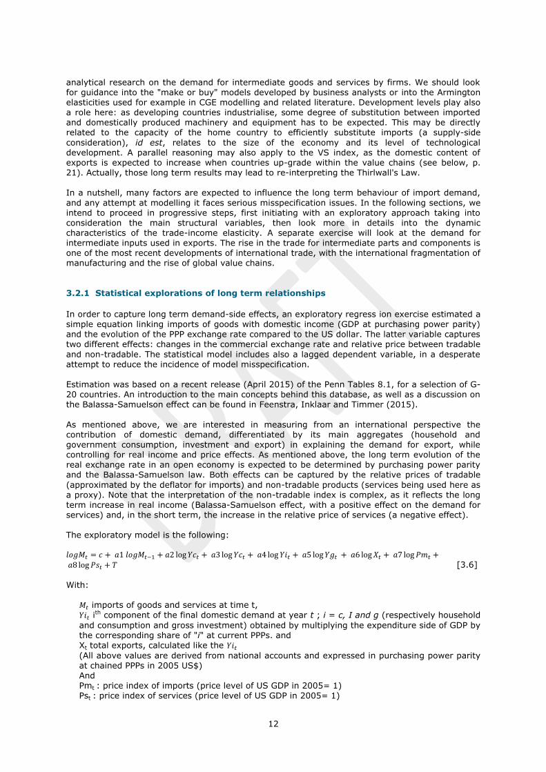
3.2.1 Statistical explorations of long term relationships

In order to capture long term demand-side effects, an exploratory regress ion exercise estimated a simple equation linking imports of goods with domestic income (GDP at purchasing power parity) and the evolution of the PPP exchange rate compared to the US dollar. The latter variable captures two different effects: changes in the commercial exchange rate and relative price between tradable

and non-tradable. The statistical model includes also a lagged dependent variable, in a desperate attempt to reduce the incidence of model misspecification. Estimation was based on a recent release (April 2015) of the Penn Tables 8.1, for a selection of G-

20 countries. An introduction to the main concepts behind this database, as well as a discussion on the Balassa-Samuelson effect can be found in Feenstra, Inklaar and Timmer (2015).

As mentioned above, we are interested in measuring from an international perspective the contribution of domestic demand, differentiated by its main aggregates (household and government consumption, investment and export) in explaining the demand for export, while controlling for real income and price effects. As mentioned above, the long term evolution of the real exchange rate in an open economy is expected to be determined by purchasing power parity and the Balassa-Samuelson law. Both effects can be captured by the relative prices of tradable

(approximated by the deflator for imports) and non-tradable products (services being used here as a proxy). Note that the interpretation of the non-tradable index is complex, as it reflects the long term increase in real income (Balassa-Samuelson effect, with a positive effect on the demand for services) and, in the short term, the increase in the relative price of services (a negative effect). The exploratory model is the following: 𝑙𝑜𝑔𝑀𝑡 = 𝑐 + 𝑎1 𝑙𝑜𝑔𝑀𝑡−1 + 𝑎2 log 𝑌𝑐𝑡 + 𝑎3 log 𝑌𝑐𝑡 + 𝑎4 log 𝑌𝑖𝑡 + 𝑎5 log 𝑌𝑔𝑡 + 𝑎6 log 𝑋𝑡 + 𝑎7 log 𝑃𝑚𝑡 + 𝑎8 log 𝑃𝑠𝑡 + 𝑇 [3.6]

With:

𝑀𝑡 imports of goods and services at time t,

𝑌𝑖𝑡 ith component of the final domestic demand at year t ; i = c, I and g (respectively household

and consumption and gross investment) obtained by multiplying the expenditure side of GDP by the corresponding share of "i" at current PPPs. and Xt total exports, calculated like the 𝑌𝑖𝑡

(All above values are derived from national accounts and expressed in purchasing power parity at chained PPPs in 2005 US$) And Pmt : price index of imports (price level of US GDP in 2005= 1) Pst : price index of services (price level of US GDP in 2005= 1)

13

T : time index, ranging from 1980 to 2011 Pst is derived from the 2005 benchmarks from Inklaar and Timmer (2012) except for Saudi Arabia where the estimate was done by the author. Other years extrapolated using deflactor for domestic absorption in the Penn World Tables 811

The lagged dependent variable 𝑀𝑡 was included for purely statistical reasons. Without it, equation

[3.6] would register high serial correlation in its residual term, indicating, inter alia, that some important missing variables were missing. Introducing the lagged dependent variable reduces the misspecification issue, and can be interpreted as an instrument capturing the idiosyncratic variables that are not well represented by country-specific dummies (fixed effects). Nevertheless, this model remains purely exploratory, its objective is to provide some magnitude about the semi-elasticity of demand for imports. Thus, statistical tests are tentative and the results should not be interpreted as confirmatory or falsification testing of pre-specified hypotheses.

A first exploration included all countries in our sample for the period 1980-2011 (Australia; Brazil; Canada; China; Germany; France; United Kingdom; Indonesia; India; Italy; Japan; Korea; Mexico;

Russia; Saudi Arabia; Turkey; United States and South Africa). In order to keep a balanced panel of observations, the Russian Federation had to be excluded for lack of data for the pre-1990 period. As our statistical foundations are shaky, we opted for OLS in order to deal more efficiently

with the probable specification and multicollinearity issues in a relatively small sample. For similar reason, our preferred model includes fixed effects (country dummies) as other idiosyncratic effects are expected to be captured by the lagged dependent variable. But this is more a wish than a fact and we also run the regression with random effects. The corresponding results can be used to check for robustness on alternative specifications [Note: this remains to be done in a revised version]. As we look for long term relationship, the model is specified in levels.

Table 2 Exploratory regressions, all countries 1980-2011

Fixed effects

a

Random effects

a

Variable Coefficient b

Std. Error

Coefficient b

Std. Error

C -1.67 0.47

-0.25 0.1

LOG M(-1) 0.52 0.03

0.76 0.02

LOG(Y_C) 0.07 0.05

0.04 0.02

LOG(Y_I) 0.14 0.03

0.05 0.02

LOG(Y_G) 0.12 0.03

0.01 0.02

LOG(X) 0.29 0.03

0.14 0.02

LOG(P_SER) 0.28 0.03

0.08 0.02

LOG(P_M) -0.32 0.06

-0.13 0.05 TREND 0.00 0.00

0.00 0.00

R-squared 0.99

0.99 Durbin-Watson stat 1.35

1.57

Notes: a/ OLS; periods included: 32 years (including 1979 for the lagged dependent variable); cross-sections included: 17; total panel (balanced) observations: 544. b/ Significant coefficients in bold (at alpha=0.05 or lower), based on t tests.

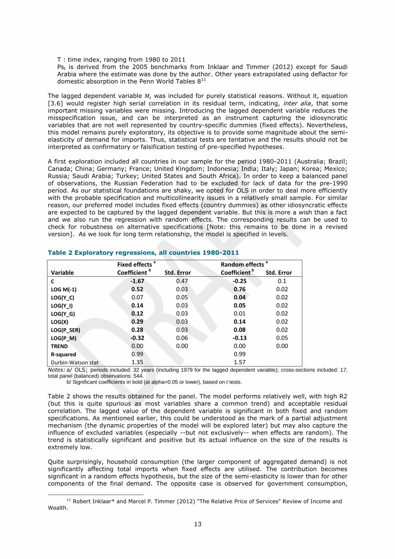
Table 2 shows the results obtained for the panel. The model performs relatively well, with high R2

(but this is quite spurious as most variables share a common trend) and acceptable residual

correlation. The lagged value of the dependent variable is significant in both fixed and random specifications. As mentioned earlier, this could be understood as the mark of a partial adjustment mechanism (the dynamic properties of the model will be explored later) but may also capture the influence of excluded variables (especially --but not exclusively-- when effects are random). The trend is statistically significant and positive but its actual influence on the size of the results is extremely low.

Quite surprisingly, household consumption (the larger component of aggregated demand) is not significantly affecting total imports when fixed effects are utilised. The contribution becomes significant in a random effects hypothesis, but the size of the semi-elasticity is lower than for other components of the final demand. The opposite case is observed for government consumption,

11 Robert Inklaar* and Marcel P. Timmer (2012) "The Relative Price of Services" Review of Income and

Wealth.

14

significant when effects are fixed but non-significant when they are random. Here again, while the coefficient is significant, it is lower than for other demand components. Investment is a clear driver of imports, and its semi-elasticity is higher than for household and government consumption. This shows the relative high import intensity of fixed capital formation, especially when it relates to machinery and equipment.

The very high semi elasticity attached to exports may be surprising at first glance, considering that global manufacturing and the increasing reliance on imported inputs to produce exports became globally significant in the mid-1990s and only for some countries (China, Europe, Mexico and the USA in particular). An additional effect is probably at work here, and relates to the Harrod tradition of export led growth in developing countries. Higher exports relax the balance of payments constraint and lead to higher domestic demand. There is therefore a pro-cyclical effect through the

financial constraint which reinforces the fact that exports are intensive in imports of intermediate inputs. The price elasticity has the expected negative coefficient. The positive coefficient associated to the

price of non-tradable (services) is also expected, but may reflect two different effects. One is the traditional relative price effect: if the relative price of non-tradable products increases, demand will tend to privilege tradable goods, and therefore boost imports. The second effect is linked to the

Balassa-Samuelson effect: the price of services (in PPP$, which means relative to the USA taken as a benchmark) reflects the increase in households' per capita income, leading to increased consumption of tradable goods even if non-tradable are superior goods under Engel's law. In the above panel regressions, all countries were pooled together; the implicit hypothesis of such grouping is that those economies differ on idiosyncratic factors (fixed or random) that affect mainly levels but share the same semi-elasticities [Note: Hypothesis to be tested in next revision].

This may not be the case, and the next exploration looks at differentiating those economies according to their development status. Table 3 compares the sets of results obtained when separating developed and developing countries.

Table 3 Exploratory regressions, developed and developing countries 1980-2011

Fixed Effects

a Random Effects

a

Developed countries

b

Developing countries

c Developed countries

b

Developing countries

c

Variable Coefficient d

Std. Err.

Coefficient

d

Std. Err. Coefficient

d

Std. Err.

Coefficient

d

Std. Err.

C -1.00 0.84

-1.47 0.68 -0.25 0.10

-0.24 0.21 LOG M(-1) 0.47 0.04

0.50 0.04 0.76 0.02

0.62 0.03

LOG(Y_C) -0.07 0.08

0.09 0.07 0.04 0.02

0.01 0.03 LOG(Y_I) 0.25 0.04

0.15 0.04 0.05 0.02

0.20 0.03

LOG(Y_G) 0.06 0.04

0.11 0.04 0.01 0.02

0.03 0.03 LOG(X) 0.36 0.03

0.27 0.04 0.14 0.02

0.14 0.03

LOG(P_SER) -0.04 0.04

0.39 0.05 0.08 0.02

0.25 0.03 LOG(P_M) -0.01 0.06

-0.40 0.09 -0.13 0.05

-0.26 0.09

TREND 0.00 0.00

0.00 0.00 0.00 0.00

0.01 0.0 R-squared 0.99

0.98

0.99

0.98

Durbin-Watson stat 1.47

1.28

1.60

1.34

Notes: a/ OLS; periods included: 32 years (including 1979 for the lagged dependent variable) b/ Cross-sections included: 8; balanced panel (8 x 32 observations) c/ Cross-sections included: 9; balanced panel (9 x 32 observations)

. d/ Significant coefficients in bold (at alpha=0.05 or lower), based on t tests.

Again, the lagged dependent variable is always significant and higher when effects are expected to be random rather than fixed The trend is positive but its economic effect is very low. Households' consumption is not a clear driver of imports, with only one case (developed countries, random

effects) where the coefficient is significantly positive. The case of government consumption is pretty similar, albeit the sole significant result is observed for developed countries (fixed effects). At the contrary, investment is intensive in imports irrespective of the sub-sample and the estimation method employed. The Harrodian perspective would have expected developing

15

economies to be more dependent of imports than industrialised economies for their investment (at least when it comes to machinery and transport equipment) but this is the case only when random effects are applied. The price of imports has the expected negative sign in all instances and appears to be more substantial for developing than developed economies. A similar result is observed for the PPP

price of services which is also a proxy for households' income. It's statistical and economic weight is much higher for developing economies than for industrial countries. This is compatible with the Balassa-Samuelson effect, stronger in developing countries (our sub-sample includes G-20 developing economies, often called "emerging"). Nevertheless, it is important to remember that all results presented here are tentative and exploratory.

3.3 Summary: main findings

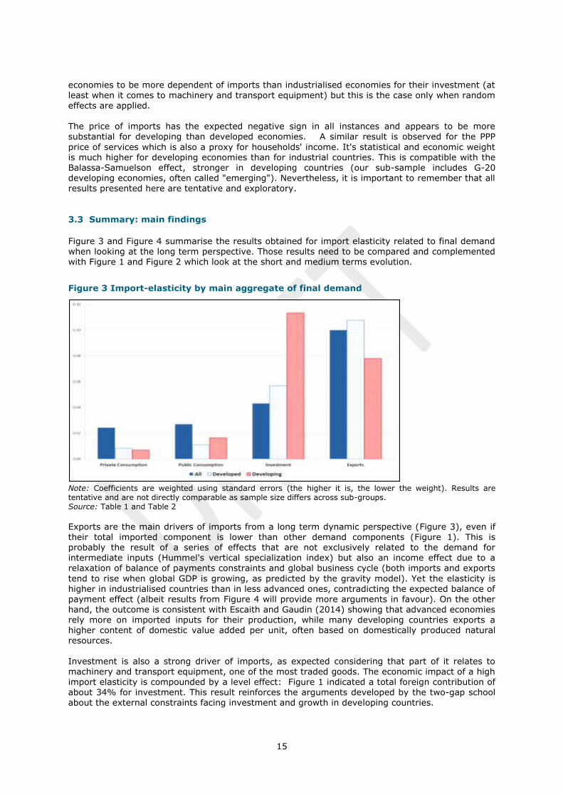
Figure 3 and Figure 4 summarise the results obtained for import elasticity related to final demand when looking at the long term perspective. Those results need to be compared and complemented with Figure 1 and Figure 2 which look at the short and medium terms evolution.

Figure 3 Import-elasticity by main aggregate of final demand

Note: Coefficients are weighted using standard errors (the higher it is, the lower the weight). Results are tentative and are not directly comparable as sample size differs across sub-groups. Source: Table 1 and Table 2

Exports are the main drivers of imports from a long term dynamic perspective (Figure 3), even if their total imported component is lower than other demand components (Figure 1). This is probably the result of a series of effects that are not exclusively related to the demand for intermediate inputs (Hummel's vertical specialization index) but also an income effect due to a

relaxation of balance of payments constraints and global business cycle (both imports and exports

tend to rise when global GDP is growing, as predicted by the gravity model). Yet the elasticity is higher in industrialised countries than in less advanced ones, contradicting the expected balance of payment effect (albeit results from Figure 4 will provide more arguments in favour). On the other hand, the outcome is consistent with Escaith and Gaudin (2014) showing that advanced economies rely more on imported inputs for their production, while many developing countries exports a higher content of domestic value added per unit, often based on domestically produced natural resources.

Investment is also a strong driver of imports, as expected considering that part of it relates to machinery and transport equipment, one of the most traded goods. The economic impact of a high import elasticity is compounded by a level effect: Figure 1 indicated a total foreign contribution of about 34% for investment. This result reinforces the arguments developed by the two-gap school about the external constraints facing investment and growth in developing countries.

16

The results obtained for household and government consumptions are less robust. Once indirect imports are included (Figure 1), household consumption is more intensive in imports (30%) than government spending (20%). The difference is due to a very low direct import component in the case of government consumption. When looking at the long term dynamics (Figure 3), the full sample estimate is higher than when developed and developing economies are split, indicating lots of variations at individual country level. Part of the issue may also be due to collinearity

(consumption is pro-cyclical); in the case of private consumption, part of the income effect may be captured by the inclusion of non-tradable price index which is strongly influenced by the Balassa-Samuelson effect.

Figure 4 Import demand and relative price elasticity

Note: Coefficients are weighted using standard errors (the higher it is, the lower the weight). Results are tentative only and are not directly comparable as sample size differs across sub-groups. Source: Table 1 and Table 2

Figure 4 summarizes the results obtained for price elasticity. As expected, imports rise when the cost of non-tradable increases and drop when their own cost rises. Developing countries are much

more sensitive to price developments than industrialised countries, perhaps because financial constraints are more binding. For services, this may also be related to the fact that the relative price of services in PPP$ captures also the change in the level of households' real income and this Balassa-Samuelson effect is expected to be higher in developing countries.

17

4 THE SUPPLY SIDE DYNAMICS

As mentioned in the introduction, long-term growth in the mainstream tradition is determined outside the GDP identity by exogenous factors affecting the supply-side of the identity, such as the increase in labour (working population), the stock of human and physical capital and technical progress. Technical progress, in turn, is a residual estimated by applying growth accounting techniques introduced by Solow in the late 1950s. From this perspective, trade promotes long

term growth by accelerating the transmission of technical progress and -- in particular when trade takes place along global value chains-- by facilitating the adoption of modern management techniques and best practices in terms of industrial norms. In addition to these effects of trade on total factor productivity (TFP), GVCs are characterized by their strong "trade-investment" nexus. Foreign Direct Investment is also a driver of growth (i) through TFP when technical progress is embodied in new generations of capital and (ii) by removing some of the balance of payment

constraints that face many developing countries.

More simply, some basic structural factors are at work to explain the relationship between world trade and world GDP reflects more structural factors. Escaith and Miroudot (2015) show that in this frictionless world, trade will grow more rapidly in the phases of GDP absolute convergence and reached a maximum when all economies are of similar size. Because trade is a driver of growth, there is an endogenous force which will sustain convergence, up to a certain level (actually, if we

follow our very simple gravity model, it is not per capital convergence which matters but market size convergence: the driving force on income will be stronger when the population is smaller). Those supply side effects are of much interest for development economists, but, when looking at the supply-side from a statistical perspective, the trade analysts focus on the specialization of each country in terms of product mix and its revealed comparative advantages. The purpose of this chapter is to look at the changes in comparative advantages that occurred during the 1995-2011

period, providing a few stylized facts and exploring the role of global value chains from a trade in value-added perspective. The calculation of Revealed Comparative Advantages (RCA) has a long story and is associated to

Balassa (1965). A similar approach, related to the Shift-Share Analysis (known as "Constant Market Share Analysis" by trade analysts), can be traced back to Tyszynski (1951). RCA looks at

the competitiveness position of an exporting country by comparing its export structure with the market structure (demand). As countries are expected to specialize in the products where they have comparative advantages, this comparison reflects its RCA. Because this analysis is based on relative market shares, it is related to the shift-share analysis which looks at decomposing trade growth through the initial distribution of market shares and a residual, supposed to measure changes in competitiveness.

During the 19th Century and most of the 20th Century, RCAs expected to show a distribution of comparative advantages closely related to the degree of industrialization, with developed countries specializing in complex manufacturing and least-advanced countries exporting commodities. In particular, export specialization as observed through trade flows is seen as a reliable indicator of a country’s underlying capabilities, conveying important information on countries’ latent capabilities (Hausmann, Hwang and Rodrik, 2007). This approach of comparative advantages

being revealed by export flows is valid when trade is composed of commodities and final goods. With the rise of GVCs, inter-industrial trade in intermediate inputs has taken much more importance, while GVCs allowed less advanced countries to leap-frog the industrialization ladder by specializing in some of the tasks required for the manufacturing of the final products. As a result, the export structure may not reflect anymore the relative situation of the exporting country with respect to the technology frontier.

As mentioned by Ferrarini and Scaramozzino (2011), today, a measure of comparative advantage that actually look at supply capabilities should be based on net trade flows at sectoral level. The analysis of RCAs on the basis of net trade flows is particularly relevant in presence of global production sharing and vertical specialization. Understanding the reality of today's trade in global manufacturing networks provides important information on the capacity for any given country to upgrade and "capture" a larger share of the value-added generated in the international supply

18

chain. 12 We propose to seize the opportunity of Trade in Value Added data allows to move the analysis one step further and include also domestic inter-industrial relationships in the analysis of comparative advantages and industrial competitiveness. 4.1 Trade in Value Added and Revealed Comparative Advantages

The TiVA database is particularly well conceived for analysing RCAs, as it is organized not according to products but according to industries. Moreover, building on the suggestion of Ferrarini and Scaramozzino (2011) but including an industry perspective rather than a product by product approach, it is possible to subtract from these exports all the imported products that a given industry required for producing its exports. This is easily done in the OECD-WTO TiVA database by taking into consideration the value of the vertical specialization (VS) index (see equation [B1.3] in

Box 1).

The calculation of RCAs is based on the comparison of export structures. In our case, we took the G-20 countries exports to the world and computed RCAs by comparing individual export structure with the G-20 average. The calculation was done for all industries (goods and services) for years 1995 and 2011. We also differentiated exports according to the use (final demand or intermediate use). This may provide interesting information on the comparative advantages relative to an

upstream or downstream position in the global value chain. Actually, according to the industry, less advanced developing countries may join either as an upstream supplier (agriculture or mining) or as downstream suppliers (final product assembly in electronics); conversely, being downstream is a sign of market power in agriculture (brand reputation associated to geographical appellations) while being upstream in electronics or automobile indicates a strong position in R&D. Due to consideration of extension, the paper will not look into the individual situation of each

sector and each country, but focus on a few stylized facts. Our first interest was to look at the changes in RCAs, and see if the initial situation in 1995 was a good predictor of achieving similar results in 2011. The results in Table 4 can be read as a kind of transition matrix, indicating the probability of maintaining the initial status over the 1995-2011 period. Overall, the odds are

clearly in favour of a conservative situation and most exporters retain their relative strengths and weaknesses.

Table 4 Correlation between sectoral comparative advantages in 1995 and in 2011

All Sectors RCA Final Goods and Services 2011

RCA Intermediate Products 2011

RCA Final Goods and Services 1995

0.7 0.6

RCA Intermediate Products 1995

0.6 0.7

Source: Based on OECD-WTO TiVA database 2015 (preliminary).

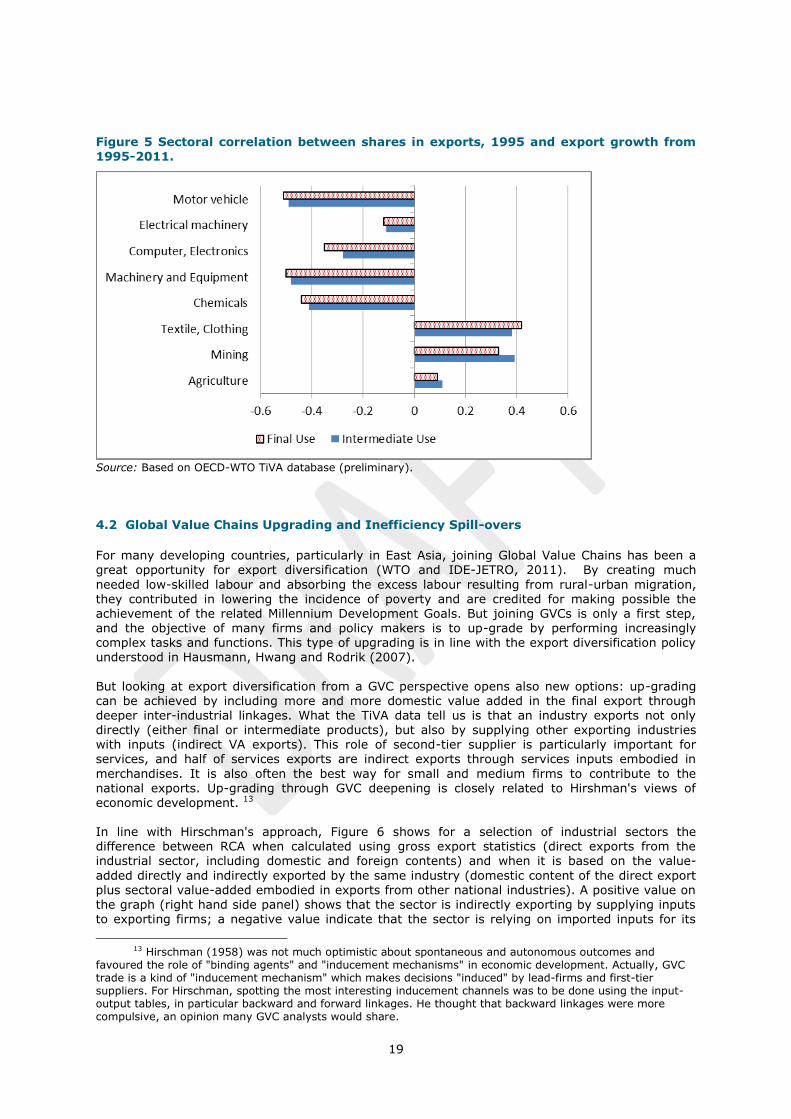
But the situation varies a lot from sector to sector. Figure 5 shows the results obtained for a selection of good producing sectors, some of them identified as low technology, others closely related to industrialization. The figure compares the initial strength in the base year with the subsequent growth of exports. Not surprisingly, natural resources rich countries maintained their

competitive advantage during the period under review, recording relatively high export growth.

But the situation was much more contrasted when we look at some industries that were particularly concerned by the global fragmentation of production. With the exception of textile and apparel, all other manufacturing sectors recorded a reversion to the mean: the dominant countries in 1995 recorded, in average, lower export growth. That the evolution of textile and apparel had, at the contrary, the effect of consolidating dominant position indicates that this sector, which was among the first one to be internationalised, had achieved its structural mutation in 1995, while

new players arrived after this date in the other industries.

12 "Capture" is not the right word when referring to GVCs, which are mainly about net value creation

and more in tune with the positive/cooperative view of the Physiocrats school than the Mercantilists' negative/confrontational vision of the world. But this zero-sum game anachronism is now firmly installed in the specialised literature, so...

19

Figure 5 Sectoral correlation between shares in exports, 1995 and export growth from 1995-2011.

Source: Based on OECD-WTO TiVA database (preliminary). 4.2 Global Value Chains Upgrading and Inefficiency Spill-overs

For many developing countries, particularly in East Asia, joining Global Value Chains has been a

great opportunity for export diversification (WTO and IDE-JETRO, 2011). By creating much

needed low-skilled labour and absorbing the excess labour resulting from rural-urban migration, they contributed in lowering the incidence of poverty and are credited for making possible the achievement of the related Millennium Development Goals. But joining GVCs is only a first step, and the objective of many firms and policy makers is to up-grade by performing increasingly complex tasks and functions. This type of upgrading is in line with the export diversification policy understood in Hausmann, Hwang and Rodrik (2007).

But looking at export diversification from a GVC perspective opens also new options: up-grading can be achieved by including more and more domestic value added in the final export through deeper inter-industrial linkages. What the TiVA data tell us is that an industry exports not only directly (either final or intermediate products), but also by supplying other exporting industries with inputs (indirect VA exports). This role of second-tier supplier is particularly important for services, and half of services exports are indirect exports through services inputs embodied in

merchandises. It is also often the best way for small and medium firms to contribute to the national exports. Up-grading through GVC deepening is closely related to Hirshman's views of

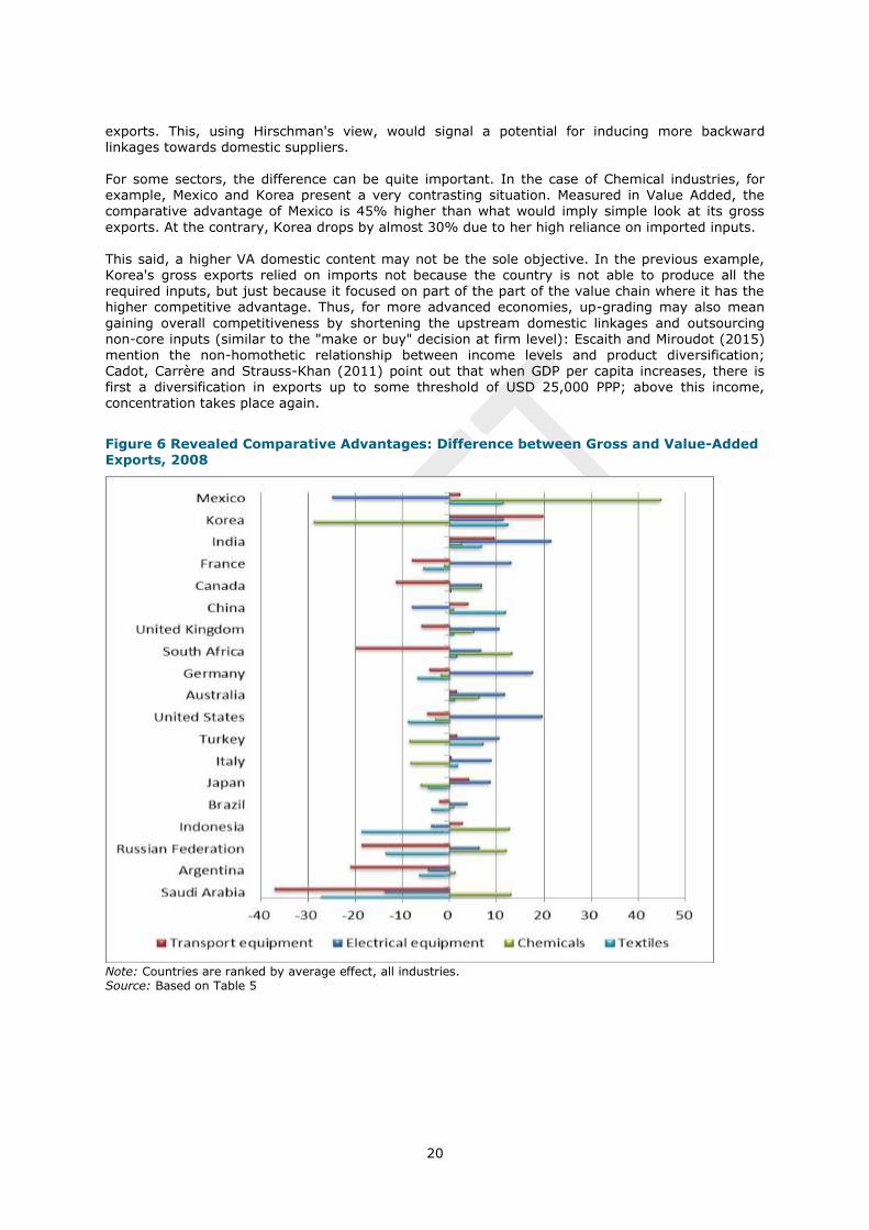
economic development. 13 In line with Hirschman's approach, Figure 6 shows for a selection of industrial sectors the difference between RCA when calculated using gross export statistics (direct exports from the industrial sector, including domestic and foreign contents) and when it is based on the value-

added directly and indirectly exported by the same industry (domestic content of the direct export plus sectoral value-added embodied in exports from other national industries). A positive value on the graph (right hand side panel) shows that the sector is indirectly exporting by supplying inputs to exporting firms; a negative value indicate that the sector is relying on imported inputs for its

13 Hirschman (1958) was not much optimistic about spontaneous and autonomous outcomes and

favoured the role of "binding agents" and "inducement mechanisms" in economic development. Actually, GVC trade is a kind of "inducement mechanism" which makes decisions "induced" by lead-firms and first-tier suppliers. For Hirschman, spotting the most interesting inducement channels was to be done using the input-output tables, in particular backward and forward linkages. He thought that backward linkages were more compulsive, an opinion many GVC analysts would share.

20

exports. This, using Hirschman's view, would signal a potential for inducing more backward linkages towards domestic suppliers. For some sectors, the difference can be quite important. In the case of Chemical industries, for example, Mexico and Korea present a very contrasting situation. Measured in Value Added, the comparative advantage of Mexico is 45% higher than what would imply simple look at its gross

exports. At the contrary, Korea drops by almost 30% due to her high reliance on imported inputs. This said, a higher VA domestic content may not be the sole objective. In the previous example, Korea's gross exports relied on imports not because the country is not able to produce all the required inputs, but just because it focused on part of the part of the value chain where it has the higher competitive advantage. Thus, for more advanced economies, up-grading may also mean

gaining overall competitiveness by shortening the upstream domestic linkages and outsourcing non-core inputs (similar to the "make or buy" decision at firm level): Escaith and Miroudot (2015) mention the non-homothetic relationship between income levels and product diversification; Cadot, Carrère and Strauss-Khan (2011) point out that when GDP per capita increases, there is

first a diversification in exports up to some threshold of USD 25,000 PPP; above this income, concentration takes place again.

Figure 6 Revealed Comparative Advantages: Difference between Gross and Value-Added Exports, 2008

Note: Countries are ranked by average effect, all industries. Source: Based on Table 5

21

Table 5 Revealed Comparative Advantage: Difference between Gross and Value-Added Exports, 2008 (in %)

Country

Avera

ge

a

Fo

od

Te

xtile

s

Wood

pro

ducts

Chem

icals

Me

tal

pro

ducts

Ma

chin

ery

Ele

ctric

al

equip

me

nt

Tra

nsport

equip

me

nt

Oth

er

ma

nufa

ctu

re

Australia -0.5 -1.5 1.0 -0.9 6.2 -6.5 -10.8 11.7 1.5 -5.2 Canada 1.0 4.1 0.3 7.5 6.8 -6.1 -3.5 6.7 -11.4 4.9 France 1.7 1.9 -5.5 3.8 -1.1 0.0 1.5 13.1 -7.9 9.7 Germany -0.5 -5.1 -6.8 -0.8 -1.8 -8.8 1.8 17.5 -4.3 4.0 Italy -1.6 -4.4 1.8 -6.4 -8.3 -5.6 -1.4 8.8 0.4 0.6 Japan -1.6 -5.5 -4.5 -3.1 -6.1 -4.5 1.1 8.6 4.0 -4.7 Korea 9.3 10.4 12.3 17.4 -28.8 -3.8 16.1 11.4 19.8 28.6 Mexico 9.6 15.6 11.4 14.1 44.7 18.9 3.6 -24.8 2.2 0.6 Turkey -1.2 5.8 7.2 -4.1 -8.5 -10.9 -2.5 10.5 1.5 -9.9 United Kingdom 0.5 0.8 0.8 1.7 5.1 -2.9 -4.8 10.4 -6.0 -0.9 United States -0.9 -10.2 -8.8 -2.4 -3.0 6.8 -5.2 19.6 -4.7 -0.7 Argentina -7.5 -5.0 -6.4 -12.0 1.2 -6.1 -8.7 -4.5 -21.0 -5.3 Brazil -3.0 -8.2 -3.8 -7.6 0.9 -0.8 -6.1 3.6 -2.2 -2.5 China 0.5 2.0 11.9 -14.6 0.9 -0.6 -3.9 -8.0 3.9 13.0 India 3.8 8.7 6.8 4.3 2.6 8.8 2.5 21.4 9.5 -30.5 Indonesia -6.3 -3.1 -18.6 -11.7 12.6 -1.4 -30.0 -3.9 2.6 -3.3 Russian Federation -6.6 -12.9 -13.5 -12.1 12.1 -0.8 -10.9 6.3 -18.6 -9.0 Saudi Arabia -25.0 -24.8 -27.3 -30.9 13.0 -44.8 -28.4 -13.7 -37.1 -31.4 South Africa -0.3 1.2 1.5 -3.0 13.1 -3.9 0.0 6.6 -19.8 2.0

Note: a: simple average of industrial sectors. All sectorial results are in percentage of the RCA calculated for Gross Exports. Source: Based on OECD-WTO TiVA, May 2013 release

4.3 GVC Up-Grading and Import-Substitution Industrialization: Old Wine in New Bottle?

Many low-income developing countries join global value chains by performing only one of the various tasks required in the global value chain. The objective of most industrial policies is to

incorporate more value-added by promoting domestic inter-industrial linkages. Adopting a value-chain perspective and developing industrial clusters, as encouraged by M. Porter (1985), has been the back-bone of many new industrial policies since the 1990s. Increasing the length of domestic supply chains and deepening backward linkages by substituting imported inputs seems very similar to the older Import Substitution Industrialization (ISI) policy pursued by many developing countries in the 1950s and still in force in some areas. Yet, there are deep differences both in the

conception and in the implementation of these policies. In the pioneering work of Michael Porter, Value Chains are not about output, they are about (consumers, stakeholders) value. Translating this approach to an inter-industrial dimension, a value-chain perspective assesses and optimizes the contribution of various industries —upstream and downstream— to the overall value. Albeit this is far from being a paradigm change from a

business perspective, looking at the creation of value rather than quantities (of production, of

employment) is probably pretty novel when designing public "industrial" policies in developing countries. It is also increasingly relevant when looking at GVCs from a "trade and development" perspective: a productive chain is as strong as its weakest part. A GVC approach to industrialization, policy-makers should design "smart industrial policies" that, at the difference of old-style vertical industrial policies, look at value creation by reducing inefficiencies. Accounting for inter-industry

linkages and sectoral inefficiencies leads to the identification of inefficiency spillovers that arise when (distorted) intermediate inputs prices (which reflect sectoral inefficiencies) transmit inefficiencies from sector to sector. The policy maker's objective should be to remove those sectoral inefficiencies in order to bring the whole domestic part of the supply chain closer to the international efficiency frontier.

22

Because (international) efficiency is only relative to (international) industrial standards, this implies comparing national industries against international benchmarks. This approach goes contrary to Import Substitution Industrial policies that were based on domestic cross-subsidies, where rents created in one productive sector would compensate for inefficiencies in others and any remaining inefficiency "paid" by final consumers. 14 At contrary, GVC approach to industrial policy means aiming at international competitiveness by optimizing each segment of the value chain

rather than looking only at the profitability of the whole process. Therefore, it is not old wine in new bottle and GVC oriented industrial policies differ from old ISI ones. Following and extending the work of Cella and Pica (2001) on 5 OECD countries, International Input-Output matrices offer a novel source of data for a worldwide efficiency benchmarking analysis, comparing domestic inter-industrial linkages for a given country against its main trade

partners. Accounting for inter-industry linkages via the IO relationship allows to track sectoral inefficiency spillovers over the upstream and downstream domestic and international segments of the value-chain.

As observed by Cella and Pica (2001), sectoral inefficiencies in the OECD were largely due to inefficiencies imported from other sectors via intermediate input prices, rather than to internal factors. Overpriced inputs may be due to technical inefficiencies affecting the upstream industrial

sectors or the effect of distorting trade policies. This is a clear indication that GVC upgrading is not a new version of ISI: In ISI, inefficient sectors were often beneficiaries of effective protection through high tariffs, resulting in final domestic prices much higher than international ones. Diakantoni and Escaith (2014) explore the impact of tariff policies on the domestic price of inputs and their cascading effect on costs of production. They show that measuring trade in value-added reveals that, in a GVC context, transaction costs (border and behind the border cost of trade) on

both imported inputs and exports are a crucial part of the competitiveness of firms and determine in part their ability to participate in production networks. In particular, tariffs have an accumulative effect with important implications on effective protection and competitiveness. Moreover, they show that domestic services producers do pay the cost of customs duties when purchasing intermediates required for their functioning; their international competitiveness and the

competitiveness of the firms they supply with their services are reduced, inducing a negative spill-

over. [Note to the First Draft: At the time of writing this document, the new release of the OECD-WTO TiVA database was still in process of finalization and we could not apply benchmarking methods to the underlying IIO data. Applying those methods, which were initially developed to compare individual firms, to input-output matrices suffers from a number of issues, linked in particular to the heterogeneity of firms within a sector or between countries. Various alternatives are available

to control for this aggregation bias and characterize metafrontiers of efficiency even in presence of heterogeneity. This remain work to be done] 5 CONCLUSIONS

After the 2008-2009 Global Crisis and its aftermath, analysing the Trade and Growth relationship

is back to fashion. This relationship is increasingly analysed through the analytical angle of global value chains which has been one of the salient feature of trade in the late 20th Century. The so-called “Glorious Fifteen” in the 1990s coincided with the rise of global manufacturing and trade along international supply chains; this period saw the emergence of large developing countries and the apparition of new key players in international economics.

We saw that North-South economic convergence by itself is a key driver of trade. In the longer term, income convergence is expected to slow-down under the force of its own success and other factors like demand switching may work in the lowering trade-income elasticity. With the rise of income, household consumption of services such as housing, health and education are expected to increase more rapidly than demand for goods. Most of these services are less tradable than

14 Inefficient sectors being often beneficiaries of effective protection through high tariffs, resulting in

final domestic prices much higher than international ones (Diakantoni and Escaith, 2014 'Trade in Tasks, Tariff Policy and Effective Protection Rates ' WTO Working Paper Series 2014-22).

23

merchandises. Even if the trade-GDP ratio stabilizes, it will do so at higher levels, increasing even more global interdependence and the demand for policy coordination. As mentioned previously, this indirect content has been increasing rapidly over the 1995-2011 period, and the 2011 value is very close to the 2008 maximum of 21%. Those findings confirm our previous hypothesis that, through its indirect content, additional public demand filters out to other countries while is apparent low import intensity makes it particularly attractive for "selfish" counter-cyclical policies.

It is therefore a good candidate for coordinated macro-policies, as policy making remains driven by domestic considerations, following the saying "economics is global but policy making is local". The supply side emphasised the differences of perception that the global value chain perspective brings when looking at export-led growth strategies and industrial policies. Even if upgrading strategies look very similar to some smart import substitution strategies as identified by

Hirschman in the late 1950s, it is not old wine in new bottles. The main difference is the constant search for efficiency which drives GVCs worldwide and should also apply at national level for the upgrading strategy to be not only sustainable, but simply doable. Identifying industrial inefficiencies is made possible by applying benchmarking techniques to international input-output

data. The source of these inefficiencies may be structural, but also linked to an outdated design of the tariff policy, inherited from the old ISI policies.

24

BIBLIOGRAPHY

Anderson, J. (2011) 'The gravity model', Annual Review of Economics 3(1), 133-160. Bacha, E. (1982) 'Growth with Limited Supplies of Foreign Exchange: a Reappraisal of the Two-

Gap Model', PUC, Rio de Janeiro. Balassa, B. (1965), Trade Liberalisation and Revealed Comparative Advantage, The Manchester

School, 33, 99-123

Balassa, B. (1964) 'The Purchasing-Power Parity Doctrine: A Reappraisal' Journal of Political Economy 72 (6): 584–96.

Cadot, O., C. Carrère and V. Strauss-Kahn (2011) 'Export diversification: what’s behind the hump?' Review of Economics and Statistics 93(2), 590–605.

Caron, J, T. Fally and J. Markusen (2014) 'International trade puzzles: a solution linking production and preferences, Quarterly Journal of Economics 129(3), 1501-1552.

Cella, G. and G. Pica (2001) 'Inefficiency Spillovers in Five OECD Countries: An Interindustry Analysis' Economic Systems Research, 13:4, 405-416

Diakantoni, A. and H. Escaith (2014) 'Trade in Tasks, Tariff Policy and Effective Protection Rates' WTO Working Paper Series 2014-22.

Escaith, H (2014) 'Mapping Global Value Chains and Measuring Trade in Tasks' in "Asia and Global Production Networks: Implications for Trade, Incomes and Economic Vulnerability" edited by B. Ferrarini and D. Hummels, Asian Development Bank and Edwar Elgar Publishing.

Escaith, H. and H, Gaudin (2014) 'Clustering Value-Added Trade: Structural and Policy Dimensions', WTO Working Paper.

Escaith, H. and S. Miroudot (2015) 'World Trade and Income Remain Exposed to Gravity', CPER eBook on Trade Peaks and Stagnation edited by Bernard Hoekman (forthcoming).

Feenstra, R; R. Inklaar and M. Timmer (2015) 'The Next Generation of the Penn World Table', Revised, April.

Ferrarini, B and P. Scaramozzino (2011) 'Indicators and Patterns of Specialization in International

Trade', NCCR Working Paper. Grossman, G. and E. Rossi-Hansberg (2006) 'The Rise of Offshoring: It’s Not Wine for Cloth

Anymore' Princeton University and Federal Reserve Bank of Kansas City, pp. 59–102. Hausmann, R., J. Hwang and D. Rodrik (2007) 'What You Export Matters' Journal of Economic

Growth, Vol. 12, pp. 1-25. Hirschman, A (1958) 'The Strategy of Economic Development' Yale Studies in Economics, Yale

University Press. Inklaar, R. and M. Timmer (2012) 'The Relative Price of Services' Review of Income and Wealth. Khan, M., and M. Goldstein (1985) 'Income and Price Effects in Foreign Trade,' in Handbook of

International Economics, volume 2, edited by Ronald Jones and Peter Kenen (New York: North Holland), pp. 1041-1105.

Kranendonk, H. and J. Verbruggen (2008) 'Decomposition of GDP growth in European countries: Different methods tell different stories' CPB Netherlands Bureau for Economic Policy Analysis

OECD-WTO (2012) 'Trade in value-added: concepts, methodologies and challenges (joint OECD-WTO note)' WTO-MIWI.

Park, A., G. Nayyar and P. Low (2013) 'Supply Chain Perspectives and Issues: A literature Review', Fung Global Institute and WTO.

Pingfan Hong (1999) 'Import Elasticities Revisited' ST/ESA/1999/DP.10 DESA Discussion Paper No. 10, United Nations.

Porter, M (1985) 'Competitive Advantage: Creating and Sustaining Superior Performance'

Samuelson, P. (1994) 'Facets of Balassa-­‐Samuelson Thirty Years Later' Review of International

Economics 2(3): 201-­‐226.

Stern, R., F. Jonathan and B. Schumacher (1976) 'Price Elasticities in International Trade—An Annotated Bibliography' (London: MacMillan).

Tyszynski, H. (1951) 'World Trade in Manufactured Commodities, 1899-1950'. The Manchester School, 19: 272–304

WTO and IDE-JETRO (2011) 'Trade Patterns and Global Value Chains in East Asia: From Trade in

Goods to Trade in Tasks', June.