23 response optimization
TRANSCRIPT
MEET MTB UGUIDE 1 SC QREFUGUIDE 2INDEXCONTENTS HOW TO USE
DOMROPTI.MK5 Page 1 Friday, December 17, 1999 1:06 PM
23Response Optimization
■ Response Optimization Overview, 23-2
■ Response Optimization, 23-2
■ Overlaid Contour Plots, 23-20
MINITAB User’s Guide 2 23-1
MEET MTB UGUIDE 1 SC QREFUGUIDE 2INDEXCONTENTS HOW TO USE
Chapter 23 Response Optimization Overview
MEET MTB UGUIDE 1 SC QREFUGUIDE 2INDEXCONTENTS HOW TO USE
DOMROPTI.MK5 Page 2 Friday, December 17, 1999 1:06 PM
Response Optimization OverviewMany designed experiments involve determining optimal conditions that will produce the “best” value for the response. Depending on the design type (factorial, response surface, or mixture), the operating conditions that you can control may include one or more of the following design variables: factors, components, process variables, or amount variables.
For example, in product development, you may need to determine the input variable settings that result in a product with desirable properties (responses). Since each property is important in determining the quality of the product, you need to consider these properties simultaneously. For example, you may want to increase the yield and decrease the cost of a chemical production process. Optimal settings of the design variables for one response may be far from optimal or even physically impossible for another response. Response optimization is a method that allows for compromise among the various responses.
MINITAB provides two commands to help you identify the combination of input variable settings that jointly optimize a set of responses. These commands can be used after you have created and analyzed factorial designs, response surface designs, and mixture designs.
■ Response Optimizer provides you with an optimal solution for the input variable combinations and an optimization plot. The optimization plot is interactive; you can adjust input variable settings on the plot to search for more desirable solutions.
■ Overlaid Contour Plot shows how each response considered relates to two continuous design variables (factorial and response surface designs) or three continuous design variables (mixture designs), while holding the other variables in the model at specified levels. The contour plot allows you to visualize an area of compromise among the various responses.
Response OptimizationYou can use MINITAB’s Response Optimizer to help identify the combination of input variable settings that jointly optimize a single response or a set of responses. Joint optimization must satisfy the requirements for all the responses in the set. The overall desirability (D) is a measure of how well you have satisfied the combined goals for all the responses. Overall desirability has a range of zero to one. One represents the ideal case; zero indicates that one or more responses are outside their acceptable limits.
MINITAB calculates an optimal solution and draws a plot. The optimal solution serves as the starting point for the plot. This optimization plot allows you to interactively change the input variable settings to perform sensitivity analyses and possibly improve the initial solution.
23-2 MINITAB User’s Guide 2
MEET MTB UGUIDE 1 SC QREFUGUIDE 2INDEXCONTENTS HOW TO USE

Response Optimization Response Optimization
MEET MTB UGUIDE 1 SC QREFUGUIDE 2INDEXCONTENTS HOW TO USE
DOMROPTI.MK5 Page 3 Friday, December 17, 1999 1:06 PM
Data
Before you use MINITAB’s Response Optimizer, you must
1 Create and store a design using one of MINITAB’s Create Design commands or create a design from data that you already have in the worksheet with Define Custom Design.
2 Enter up to 25 numeric response columns in the worksheet.
3 Fit a model for each response using one of the following:
You can fit a model with different design variables for each response. If an input variable was not included in the model for a particular response, the optimization plot for that response-input variable combination will be blank.
MINITAB automatically omits missing data from the calculations. If you optimize more than one response and there are missing data, MINITAB excludes the row with missing data from calculations for all of the responses.
Note Although numerical optimization along with graphical analysis can provide useful information, it is not a substitute for subject matter expertise. Be sure to use relevant background information, theoretical principles, and knowledge gained through observation or previous experimentation when applying these methods.
Command on page…
Create Factorial Design 19-6, 19-24
Create Response Surface Design 20-4
Create Mixture Design 21-5
Define Custom Factorial Design 19-35
Define Custom Response Surface Design 20-19
Define Custom Mixture Design 21-28
Command on page…
Analyze Factorial Design 19-44
Analyze Response Surface Design 20-26
Analyze Mixture Design 21-38
Note Response Optimization is not available for general full factorial designs.
MINITAB User’s Guide 2 23-3
MEET MTB UGUIDE 1 SC QREFUGUIDE 2INDEXCONTENTS HOW TO USE
Chapter 23 Response Optimization
MEET MTB UGUIDE 1 SC QREFUGUIDE 2INDEXCONTENTS HOW TO USE
DOMROPTI.MK5 Page 4 Friday, December 17, 1999 1:06 PM
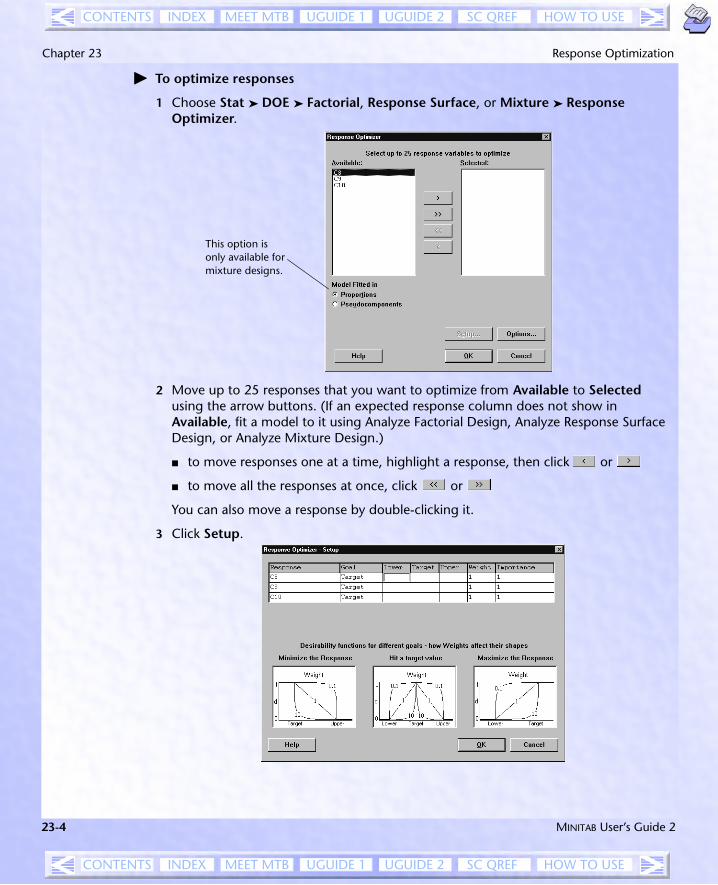
h To optimize responses
1 Choose Stat ➤ DOE ➤ Factorial, Response Surface, or Mixture ➤ Response Optimizer.
2 Move up to 25 responses that you want to optimize from Available to Selected using the arrow buttons. (If an expected response column does not show in Available, fit a model to it using Analyze Factorial Design, Analyze Response Surface Design, or Analyze Mixture Design.)
■ to move responses one at a time, highlight a response, then click or
■ to move all the responses at once, click or
You can also move a response by double-clicking it.
3 Click Setup.
This option is only available for mixture designs.
23-4 MINITAB User’s Guide 2
MEET MTB UGUIDE 1 SC QREFUGUIDE 2INDEXCONTENTS HOW TO USE

Response Optimization Response Optimization
MEET MTB UGUIDE 1 SC QREFUGUIDE 2INDEXCONTENTS HOW TO USE
DOMROPTI.MK5 Page 5 Friday, December 17, 1999 1:06 PM
4 For each response, complete the table as follows:
■ Under Goal, choose Minimize, Target, or Maximize from the drop-down list.
■ Under Lower, Target, and Upper, enter numeric values for the target and necessary bounds as follows:
1 If you choose Minimize under Goal, enter values in Target and Upper.
2 If you choose Target under Goal, enter values in Lower, Target, and Upper.3 If you choose Maximize under Goal, enter values in Target and Lower.
For guidance on choosing bounds, see Specifying bounds on page 23-7.
■ In Weight, enter a number from 0.1 to 10 to define the shape of the desirability function. See Setting the weight for the desirability function on page 23-9.
■ In Importance, enter a number from 0.1 to 10 to specify the relative importance of the response. See Specifying the importance for composite desirability on page 23-11.
4 Click OK.
5 If you like, use any of the options listed below, then click OK.
Options
Response Optimizer dialog box
■ for mixture designs, refit the model in proportions or psuedocomponents.
Options subdialog box
■ define a starting point for the search algorithm by providing a value for each input variable in your model. Each value must be between the minimum and maximum levels for that input variable.
■ for factorial designs, define settings at which to hold any covariates that are in the model.
■ suppress display of the multiple response optimization plot.
■ store the composite desirability values.
■ display local solutions.
Response optimization plot
■ adjust input variable settings interactively. You can also– save new input variable settings– delete saved input variable settings– reset optimization plot to initial or optimal settings– view a list of all saved settings– for mixture designs, lock component values
MINITAB User’s Guide 2 23-5
MEET MTB UGUIDE 1 SC QREFUGUIDE 2INDEXCONTENTS HOW TO USE
Chapter 23 Response Optimization
MEET MTB UGUIDE 1 SC QREFUGUIDE 2INDEXCONTENTS HOW TO USE
DOMROPTI.MK5 Page 6 Friday, December 17, 1999 1:06 PM
See Using the optimization plot on page 23-11.
Method
MINITAB’s Response Optimizer searches for a combination of input variable levels that jointly optimize a set of responses by satisfying the requirements for each response in the set. The optimization is accomplished by
1 obtaining the individual desirability (d) for each response
2 combining the individual desirabilities to obtain the combined or composite desirability (D)
3 maximizing the composite desirability and identifying the optimal input variable settings
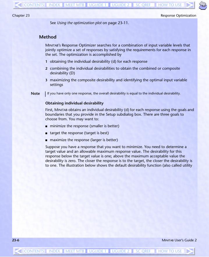
Obtaining individual desirability
First, MINITAB obtains an individual desirability (d) for each response using the goals and boundaries that you provide in the Setup subdialog box. There are three goals to choose from. You may want to:
■ minimize the response (smaller is better)
■ target the response (target is best)
■ maximize the response (larger is better)
Suppose you have a response that you want to minimize. You need to determine a target value and an allowable maximum response value. The desirability for this response below the target value is one; above the maximum acceptable value the desirability is zero. The closer the response is to the target, the closer the desirability is to one. The illustration below shows the default desirability function (also called utility
Note If you have only one response, the overall desirability is equal to the individual desirability.
23-6 MINITAB User’s Guide 2
MEET MTB UGUIDE 1 SC QREFUGUIDE 2INDEXCONTENTS HOW TO USE
Response Optimization Response Optimization
MEET MTB UGUIDE 1 SC QREFUGUIDE 2INDEXCONTENTS HOW TO USE
DOMROPTI.MK5 Page 7 Friday, December 17, 1999 1:06 PM
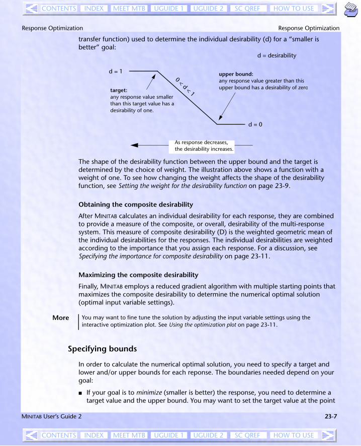
transfer function) used to determine the individual desirability (d) for a “smaller is better” goal:
The shape of the desirability function between the upper bound and the target is determined by the choice of weight. The illustration above shows a function with a weight of one. To see how changing the weight affects the shape of the desirability function, see Setting the weight for the desirability function on page 23-9.
Obtaining the composite desirability
After MINITAB calculates an individual desirability for each response, they are combined to provide a measure of the composite, or overall, desirability of the multi-response system. This measure of composite desirability (D) is the weighted geometric mean of the individual desirabilities for the responses. The individual desirabilities are weighted according to the importance that you assign each response. For a discussion, see Specifying the importance for composite desirability on page 23-11.
Maximizing the composite desirability
Finally, MINITAB employs a reduced gradient algorithm with multiple starting points that maximizes the composite desirability to determine the numerical optimal solution (optimal input variable settings).
Specifying bounds
In order to calculate the numerical optimal solution, you need to specify a target and lower and/or upper bounds for each reponse. The boundaries needed depend on your goal:
■ If your goal is to minimize (smaller is better) the response, you need to determine a target value and the upper bound. You may want to set the target value at the point
d = 0
d = 1 upper bound:any response value greater than this upper bound has a desirability of zerotarget:
any response value smaller than this target value has a desirability of one.
As response decreases, the desirability increases.
0 < d < 1
d = desirability
More You may want to fine tune the solution by adjusting the input variable settings using the interactive optimization plot. See Using the optimization plot on page 23-11.
MINITAB User’s Guide 2 23-7
MEET MTB UGUIDE 1 SC QREFUGUIDE 2INDEXCONTENTS HOW TO USE

Chapter 23 Response Optimization
MEET MTB UGUIDE 1 SC QREFUGUIDE 2INDEXCONTENTS HOW TO USE
DOMROPTI.MK5 Page 8 Friday, December 17, 1999 1:06 PM
of diminishing returns, that is, although you want to minimize the response, going below a certain value makes little or no difference. If there is no point of diminishing returns, use a very small number, one that is probably not achievable, for the target value.
■ If your goal is to target the response, you probably have upper and lower specification limits for the response that can be used as lower and upper bounds.
■ If your goal is to maximize (larger is better) the response, you need to determine a target value and the lower bound. Again, you may want to set the target value at the point of diminishing returns, although now you need a value on the upper end instead of the lower end of the range.
23-8 MINITAB User’s Guide 2
MEET MTB UGUIDE 1 SC QREFUGUIDE 2INDEXCONTENTS HOW TO USE
Response Optimization Response Optimization
MEET MTB UGUIDE 1 SC QREFUGUIDE 2INDEXCONTENTS HOW TO USE
DOMROPTI.MK5 Page 9 Friday, December 17, 1999 1:06 PM
Setting the weight for the desirability function
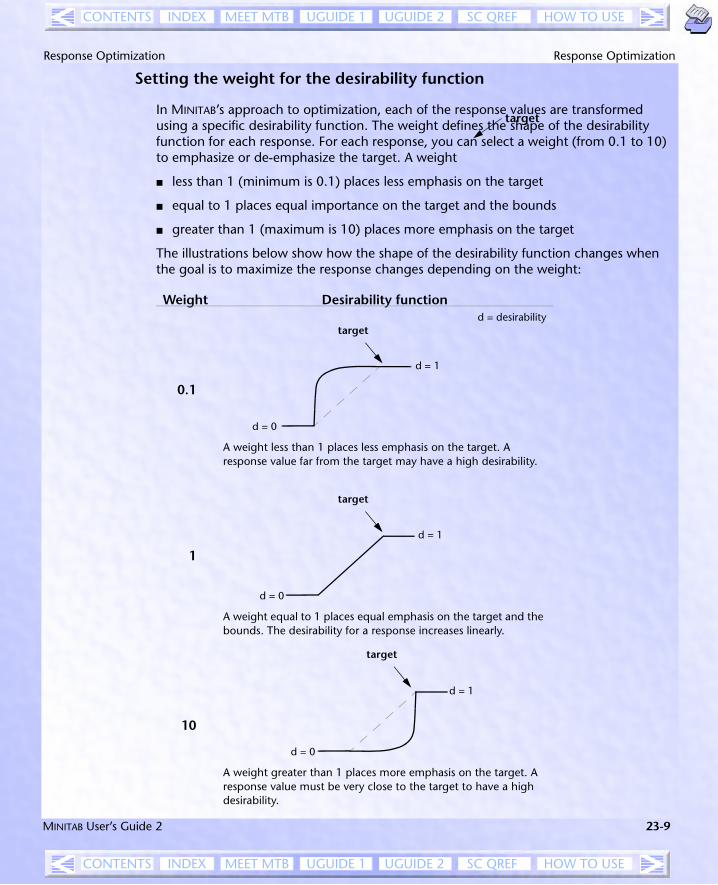
In MINITAB’s approach to optimization, each of the response values are transformed using a specific desirability function. The weight defines the shape of the desirability function for each response. For each response, you can select a weight (from 0.1 to 10) to emphasize or de-emphasize the target. A weight
■ less than 1 (minimum is 0.1) places less emphasis on the target
■ equal to 1 places equal importance on the target and the bounds
■ greater than 1 (maximum is 10) places more emphasis on the target
The illustrations below show how the shape of the desirability function changes when the goal is to maximize the response changes depending on the weight:
Weight Desirability function
0.1
d = desirability
A weight less than 1 places less emphasis on the target. A response value far from the target may have a high desirability.
1
A weight equal to 1 places equal emphasis on the target and the bounds. The desirability for a response increases linearly.
10
A weight greater than 1 places more emphasis on the target. A response value must be very close to the target to have a high desirability.
target
d = 0
d = 1
target
d = 0
d = 1
d = 0
d = 1
target
target
MINITAB User’s Guide 2 23-9
MEET MTB UGUIDE 1 SC QREFUGUIDE 2INDEXCONTENTS HOW TO USE
Chapter 23 Response Optimization
MEET MTB UGUIDE 1 SC QREFUGUIDE 2INDEXCONTENTS HOW TO USE
DOMROPTI.MK5 Page 10 Friday, December 17, 1999 1:06 PM
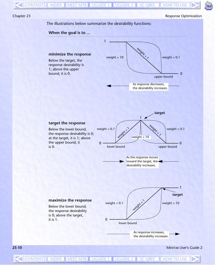
The illustrations below summarize the desirability functions:
When the goal is to ...
minimize the response
Below the target, the response desirability is 1; above the upper bound, it is 0.
target the response
Below the lower bound, the response desirability is 0; at the target, it is 1; above the upper bound, it is 0.
maximize the response
Below the lower bound, the response desirability is 0; above the target, it is 1.
0
1
weight = 10 weight = 0.1
weight = 1
upper bound
As response decreases, the desirability increases.
0
1
0
target
weight =
1weight = 1
lower bound upper bound
weight = 0.1weight = 0.1
weight = 10
As the response moves toward the target, the desirability increases.
0
1
lower bound
weight = 0.1 weight = 10
weight =
1
target
As response increases, the desirability increases.
23-10 MINITAB User’s Guide 2
MEET MTB UGUIDE 1 SC QREFUGUIDE 2INDEXCONTENTS HOW TO USE

Response Optimization Response Optimization
MEET MTB UGUIDE 1 SC QREFUGUIDE 2INDEXCONTENTS HOW TO USE
DOMROPTI.MK5 Page 11 Friday, December 17, 1999 1:06 PM
Specifying the importance for composite desirability
After MINITAB calculates individual desirabilities for the responses, they are combined to provide a measure of the composite, or overall, desirability of the multi-response system. This measure of composite desirability is the weighted geometric mean of the individual desirabilities for the responses. The optimal solution (optimal operating conditions) can then be determined by maximizing the composite desirability.
You need to assess the importance of each response in order to assign appropriate values. Importance values must be between 0.1 and 10. If all responses are equally important, use the default value of 1.0 for each response. The composite desirability is then the geometric mean of the individual desirabilities.
However, if some responses are more important than others, you can incorporate this information into the optimal solution by setting unequal importance values. Larger values correspond to more important responses, smaller values to less important responses.
You can also change the importance to determine how sensitive the solution is to the assigned values. For example, you may find that the optimal solution when one response has a greater importance is very different from the optimal solution when the same response has a lesser importance.
Using the optimization plot
Once you have created an optimization plot, you can change the input variable settings. For factorial and response surface designs, you can adjust the factor levels. For mixture designs, you can adjust component, process variable, and amount variable settings. You might want to change these input variable settings on the optimization plot for many reasons, including
■ to search for input variable settings with a higher composite desirability
■ to search for lower-cost input variable settings with near optimal properties
■ to explore the sensitivity of response variables to changes in the design variables
■ to “calculate” the predicted responses for an input variable setting of interest
■ to explore input variable settings in the neighborhood of a local solution
When you change an input variable to a new level, the graphs are redrawn and the predicted responses and desirabilities are recalculated. If you discover a setting combination that has a composite desirability higher than the initial optimal setting, MINITAB replaces the initial optimal setting with the new optimal setting. You will then have the option of adding the previous optimal setting to the saved settings list.
MINITAB User’s Guide 2 23-11
MEET MTB UGUIDE 1 SC QREFUGUIDE 2INDEXCONTENTS HOW TO USE
Chapter 23 Response Optimization
MEET MTB UGUIDE 1 SC QREFUGUIDE 2INDEXCONTENTS HOW TO USE
DOMROPTI.MK5 Page 12 Friday, December 17, 1999 1:06 PM
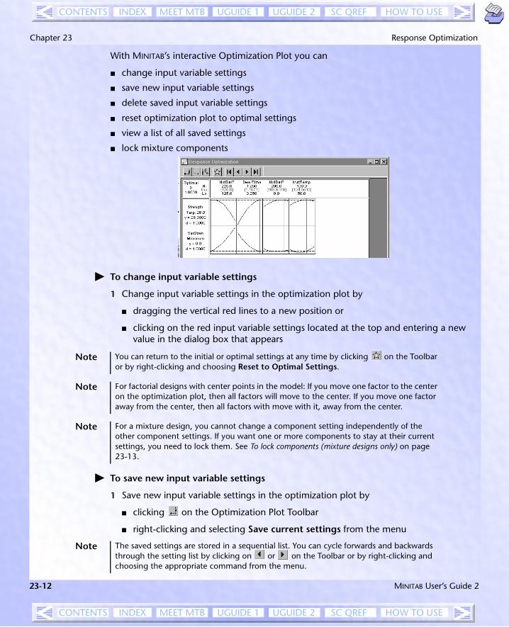
With MINITAB’s interactive Optimization Plot you can
■ change input variable settings
■ save new input variable settings
■ delete saved input variable settings
■ reset optimization plot to optimal settings
■ view a list of all saved settings
■ lock mixture components
h To change input variable settings
1 Change input variable settings in the optimization plot by
■ dragging the vertical red lines to a new position or
■ clicking on the red input variable settings located at the top and entering a new value in the dialog box that appears
h To save new input variable settings
1 Save new input variable settings in the optimization plot by
■ clicking on the Optimization Plot Toolbar
■ right-clicking and selecting Save current settings from the menu
Note You can return to the initial or optimal settings at any time by clicking on the Toolbar or by right-clicking and choosing Reset to Optimal Settings.
Note For factorial designs with center points in the model: If you move one factor to the center on the optimization plot, then all factors will move to the center. If you move one factor away from the center, then all factors with move with it, away from the center.
Note For a mixture design, you cannot change a component setting independently of the other component settings. If you want one or more components to stay at their current settings, you need to lock them. See To lock components (mixture designs only) on page 23-13.
Note The saved settings are stored in a sequential list. You can cycle forwards and backwards through the setting list by clicking on or on the Toolbar or by right-clicking and choosing the appropriate command from the menu.
23-12 MINITAB User’s Guide 2
MEET MTB UGUIDE 1 SC QREFUGUIDE 2INDEXCONTENTS HOW TO USE

Response Optimization Response Optimization
MEET MTB UGUIDE 1 SC QREFUGUIDE 2INDEXCONTENTS HOW TO USE
DOMROPTI.MK5 Page 13 Friday, December 17, 1999 1:06 PM
h To delete saved input variable settings
1 Choose the setting that you want to delete by cycling through the list.
2 Delete the setting by
■ clicking on the Optimization Plot Toolbar
■ right-clicking and choosing Delete Current Setting
h To reset optimization plot to optimal settings
1 Reset to optimal settings by
■ clicking on the Toolbar
■ right-clicking and choosing Reset to Optimal Settings
h To lock components (mixture designs only)
1 Lock a component by clicking on the black [ ] before the component name. You cannot lock a component at a value that would prevent any other component from changing. In addition, you must leave at least two components unlocked.
h To view a list of all saved settings
1 View the a list of all saved settings by
■ clicking on the Optimization Plot Toolbar
■ right-clicking and choosing Display Settings List
e Example of a response optimization experiment for a factorial design
You are an engineer assigned to optimize the responses from a chemical reaction experiment. You have determined that three factors—reaction time, reaction temperature, and type of catalyst—affect the yield and cost of the process. You want to find the factor settings that maximize the yield and minimize the cost of the process.
1 Open the worksheet FACTOPT.MTW. (We have saved the design, response data, and model information for you.)
2 Choose Stat ➤ DOE ➤ Factorial ➤ Response Optimizer.
3 Click to move Yield and Cost to Selected.
More You can copy the saved setting list to the Clipboard by right-clicking and choosing Select All and then choosing Copy.
MINITAB User’s Guide 2 23-13
MEET MTB UGUIDE 1 SC QREFUGUIDE 2INDEXCONTENTS HOW TO USE

Chapter 23 Response Optimization
MEET MTB UGUIDE 1 SC QREFUGUIDE 2INDEXCONTENTS HOW TO USE
DOMROPTI.MK5 Page 14 Friday, December 17, 1999 1:06 PM
4 Click Setup. Complete the Goal, Lower, Target, and Upper columns of the table as shown below:
5 Click OK in each dialog box.
Sessionwindowoutput
Response Optimization
Parameters
Goal Lower Target Upper Weight ImportYield Maximum 35 45 45 1 1Cost Minimum 28 28 35 1 1
Global Solution
Time = 46.062Temp = 150.000Catalyst = -1.000 (A)
Predicted Responses
Yield = 44.8077, desirability = 0.98077Cost = 28.9005, desirability = 0.87136
Composite Desirability = 0.92445
Interpreting results
The individual desirability for Yield is 0.98081; the individual desirability for Cost is 0.87132. The composite desirability for both these two variables is 0.92445.
To obtain this desirability, you would set the factor levels at the values shown under Global Solution in the Session window. That is, time would be set at 46.062, temperature at 150, and you would use catalyst A.
Response Goal Lower Target Upper
Yield Maximize 35 45
Cost Minimize 28 35
Graphwindowoutput
23-14 MINITAB User’s Guide 2
MEET MTB UGUIDE 1 SC QREFUGUIDE 2INDEXCONTENTS HOW TO USE
Response Optimization Response Optimization
MEET MTB UGUIDE 1 SC QREFUGUIDE 2INDEXCONTENTS HOW TO USE
DOMROPTI.MK5 Page 15 Friday, December 17, 1999 1:06 PM
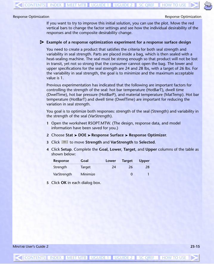
If you want to try to improve this initial solution, you can use the plot. Move the red vertical bars to change the factor settings and see how the individual desirability of the responses and the composite desirability change.
e Example of a response optimization experiment for a response surface design
You need to create a product that satisfies the criteria for both seal strength and variability in seal strength. Parts are placed inside a bag, which is then sealed with a heat-sealing machine. The seal must be strong enough so that product will not be lost in transit, yet not so strong that the consumer cannot open the bag. The lower and upper specifications for the seal strength are 24 and 28 lbs, with a target of 26 lbs. For the variability in seal strength, the goal is to minimize and the maximum acceptable value is 1.
Previous experimentation has indicated that the following are important factors for controlling the strength of the seal: hot bar temperature (HotBarT), dwell time (DwelTime), hot bar pressure (HotBarP), and material temperature (MatTemp). Hot bar temperature (HotBarT) and dwell time (DwelTime) are important for reducing the variation in seal strength.
You goal is to optimize both responses: strength of the seal (Strength) and variability in the strength of the seal (VarStrength).
1 Open the worksheet RSOPT.MTW. (The design, response data, and model information have been saved for you.)
2 Choose Stat ➤ DOE ➤ Response Surface ➤ Response Optimizer.
3 Click to move Strength and VarStrength to Selected.
4 Click Setup. Complete the Goal, Lower, Target, and Upper columns of the table as shown below:
5 Click OK in each dialog box.
Response Goal Lower Target Upper
Strength Target 24 26 28
VarStrength Minimize 0 1
MINITAB User’s Guide 2 23-15
MEET MTB UGUIDE 1 SC QREFUGUIDE 2INDEXCONTENTS HOW TO USE
Chapter 23 Response Optimization
MEET MTB UGUIDE 1 SC QREFUGUIDE 2INDEXCONTENTS HOW TO USE
DOMROPTI.MK5 Page 16 Friday, December 17, 1999 1:06 PM
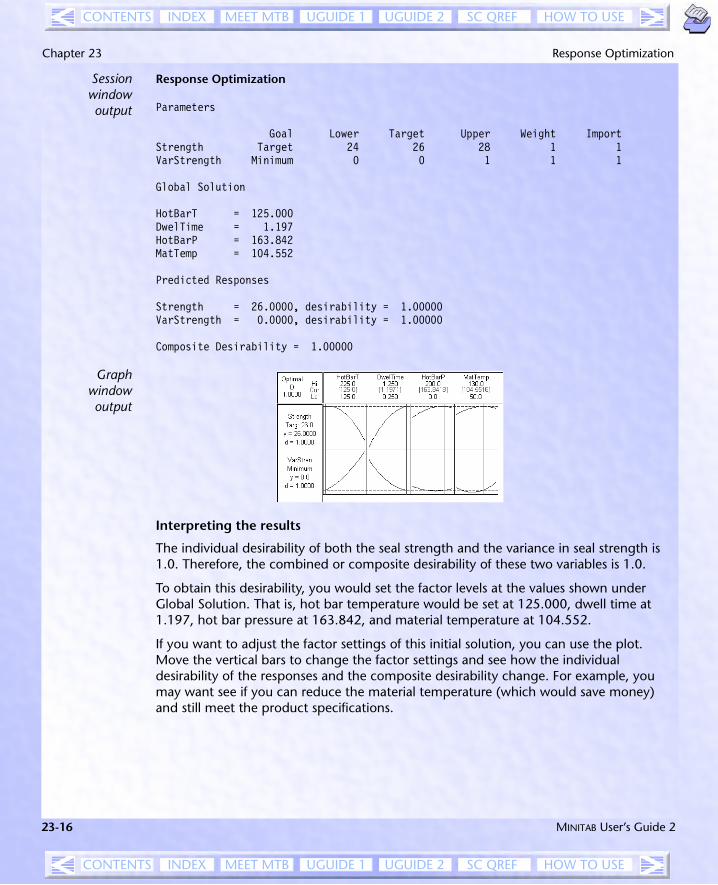
Sessionwindowoutput
Response Optimization
Parameters
Goal Lower Target Upper Weight ImportStrength Target 24 26 28 1 1VarStrength Minimum 0 0 1 1 1
Global Solution
HotBarT = 125.000DwelTime = 1.197HotBarP = 163.842MatTemp = 104.552
Predicted Responses
Strength = 26.0000, desirability = 1.00000VarStrength = 0.0000, desirability = 1.00000
Composite Desirability = 1.00000
Interpreting the results
The individual desirability of both the seal strength and the variance in seal strength is 1.0. Therefore, the combined or composite desirability of these two variables is 1.0.
To obtain this desirability, you would set the factor levels at the values shown under Global Solution. That is, hot bar temperature would be set at 125.000, dwell time at 1.197, hot bar pressure at 163.842, and material temperature at 104.552.
If you want to adjust the factor settings of this initial solution, you can use the plot. Move the vertical bars to change the factor settings and see how the individual desirability of the responses and the composite desirability change. For example, you may want see if you can reduce the material temperature (which would save money) and still meet the product specifications.
Graphwindowoutput
23-16 MINITAB User’s Guide 2
MEET MTB UGUIDE 1 SC QREFUGUIDE 2INDEXCONTENTS HOW TO USE
Response Optimization Response Optimization
MEET MTB UGUIDE 1 SC QREFUGUIDE 2INDEXCONTENTS HOW TO USE
DOMROPTI.MK5 Page 17 Friday, December 17, 1999 1:06 PM
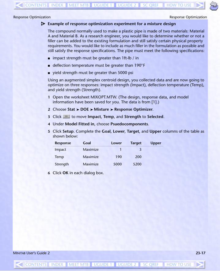
e Example of response optimization experiment for a mixture design
The compound normally used to make a plastic pipe is made of two materials: Material A and Material B. As a research engineer, you would like to determine whether or not a filler can be added to the existing formulation and still satisfy certain physical property requirements. You would like to include as much filler in the formulation as possible and still satisfy the response specifications. The pipe must meet the following specifications:
■ impact strength must be greater than 1ft-lb / in
■ deflection temperature must be greater than 190°F
■ yield strength must be greater than 5000 psi
Using an augmented simplex centroid design, you collected data and are now going to optimize on three responses: impact strength (Impact), deflection temperature (Temp), and yield strength (Strength).
1 Open the worksheet MIXOPT.MTW. (The design, response data, and model information have been saved for you. The data is from [1].)
2 Choose Stat ➤ DOE ➤ Mixture ➤ Response Optimizer.
3 Click to move Impact, Temp, and Strength to Selected.
4 Under Model Fitted in, choose Psuedocomponents.
5 Click Setup. Complete the Goal, Lower, Target, and Upper columns of the table as shown below:
6 Click OK in each dialog box.
Response Goal Lower Target Upper
Impact Maximize 1 3
Temp Maximize 190 200
Strength Maximize 5000 5200
MINITAB User’s Guide 2 23-17
MEET MTB UGUIDE 1 SC QREFUGUIDE 2INDEXCONTENTS HOW TO USE

Chapter 23 Response Optimization
MEET MTB UGUIDE 1 SC QREFUGUIDE 2INDEXCONTENTS HOW TO USE
DOMROPTI.MK5 Page 18 Friday, December 17, 1999 1:06 PM
Sessionwindowoutput
Response Optimization
Parameters
Goal Lower Target Upper Weight ImportImpact Maximum 1 3 3 1 1Temp Maximum 190 200 200 1 1Strength Maximum 5000 5200 5200 1 1
Global Solution
Components
Mat-A = 0.575Mat-B = 0.425Filler = 0.000
Predicted Responses
Impact = 7.26, desirability = 1Temp = 203.93, desirability = 1Strength = 5255.47, desirability = 1
Composite Desirability = 1.00000
Graphwindowoutput
23-18 MINITAB User’s Guide 2
MEET MTB UGUIDE 1 SC QREFUGUIDE 2INDEXCONTENTS HOW TO USE
Response Optimization Response Optimization
MEET MTB UGUIDE 1 SC QREFUGUIDE 2INDEXCONTENTS HOW TO USE
DOMROPTI.MK5 Page 19 Friday, December 17, 1999 1:06 PM
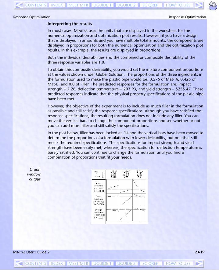
Interpreting the results
In most cases, MINITAB uses the units that are displayed in the worksheet for the numerical optimization and optimization plot results. However, if you have a design that is displayed in amounts and you have multiple total amounts, the components are displayed in proportions for both the numerical optimization and the optimization plot results. In this example, the results are displayed in proportions.
Both the individual desirabilities and the combined or composite desirability of the three response variables are 1.0.
To obtain this composite desirability, you would set the mixture component proportions at the values shown under Global Solution. The proportions of the three ingredients in the formulation used to make the plastic pipe would be: 0.575 of Mat- A; 0.425 of Mat-B, and 0.0 of Filler. The predicted responses for the formulation are: impact strength = 7.26, deflection temperature = 203.93, and yield strength = 5255.47. These predicted responses indicate that the physical property specifications of the plastic pipe have been met.
However, the objective of the experiment is to include as much filler in the formulation as possible and still satisfy the response specifications. Although you have satisfied the response specifications, the resulting formulation does not include any filler. You can move the vertical bars to change the component proportions and see whether or not you can add more filler and still satisfy the specifications.
In the plot below, filler has been locked at .14 and the vertical bars have been moved to determine the proportions of a formulation with lower desirability, but one that still meets the required specifications. The specifications for impact strength and yield strength have been easily met, whereas, the specification for deflection temperature is barely satisfied. You can continue to change the formulation until you find a combination of proportions that fit your needs.
Graphwindowoutput
MINITAB User’s Guide 2 23-19
MEET MTB UGUIDE 1 SC QREFUGUIDE 2INDEXCONTENTS HOW TO USE
Chapter 23 Overlaid Contour Plots
MEET MTB UGUIDE 1 SC QREFUGUIDE 2INDEXCONTENTS HOW TO USE
DOMROPTI.MK5 Page 20 Friday, December 17, 1999 1:06 PM
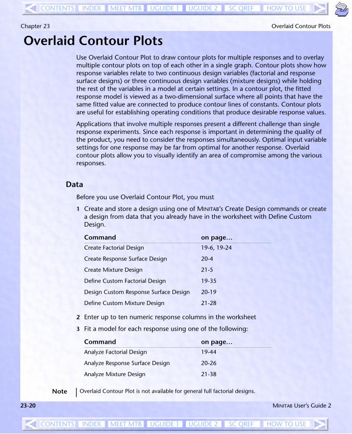
Overlaid Contour PlotsUse Overlaid Contour Plot to draw contour plots for multiple responses and to overlay multiple contour plots on top of each other in a single graph. Contour plots show how response variables relate to two continuous design variables (factorial and response surface designs) or three continuous design variables (mixture designs) while holding the rest of the variables in a model at certain settings. In a contour plot, the fitted response model is viewed as a two-dimensional surface where all points that have the same fitted value are connected to produce contour lines of constants. Contour plots are useful for establishing operating conditions that produce desirable response values.
Applications that involve multiple responses present a different challenge than single response experiments. Since each response is important in determining the quality of the product, you need to consider the responses simultaneously. Optimal input variable settings for one response may be far from optimal for another response. Overlaid contour plots allow you to visually identify an area of compromise among the various responses.
Data
Before you use Overlaid Contour Plot, you must
1 Create and store a design using one of MINITAB’s Create Design commands or create a design from data that you already have in the worksheet with Define Custom Design.
2 Enter up to ten numeric response columns in the worksheet
3 Fit a model for each response using one of the following:
Command on page…
Create Factorial Design 19-6, 19-24
Create Response Surface Design 20-4
Create Mixture Design 21-5
Define Custom Factorial Design 19-35
Design Custom Response Surface Design 20-19
Define Custom Mixture Design 21-28
Command on page…
Analyze Factorial Design 19-44
Analyze Response Surface Design 20-26
Analyze Mixture Design 21-38
Note Overlaid Contour Plot is not available for general full factorial designs.
23-20 MINITAB User’s Guide 2
MEET MTB UGUIDE 1 SC QREFUGUIDE 2INDEXCONTENTS HOW TO USE

Overlaid Contour Plots Response Optimization
MEET MTB UGUIDE 1 SC QREFUGUIDE 2INDEXCONTENTS HOW TO USE
DOMROPTI.MK5 Page 21 Friday, December 17, 1999 1:06 PM
h To draw an overlaid contour plot
1 Choose Stat ➤ DOE ➤ Factorial, Response Surface, or Mixture ➤ Overlaid Contour Plot.
2 Under Responses, move up to ten responses that you want to include in the plot from Available to Selected using the arrow buttons.
■ To move the responses one at a time, highlight a response, then click or
■ To move all of the responses, click on or
You can also move a response by double-clicking it.
3 Do one of the following:
■ For factorial and response surface designs, under Factors, choose a factor from X Axis and a factor from Y Axis.
■ For a mixture design, do one of the following:
1 To plot components, under Select components or process variables as axes, choose 3 Components. Then choose a component from X Axis, Y Axis, and Z Axis.
2 To plot process variables, under Select components or process variables as axes, choose 2 process variables.
Factorial andResponse Surface Designs Mixture Designs
Note Only numeric factors are valid candidates for X and Y axes.
Note Only numeric process variables are valid candidates for X and Y axes.
MINITAB User’s Guide 2 23-21
MEET MTB UGUIDE 1 SC QREFUGUIDE 2INDEXCONTENTS HOW TO USE

Chapter 23 Overlaid Contour Plots
MEET MTB UGUIDE 1 SC QREFUGUIDE 2INDEXCONTENTS HOW TO USE
DOMROPTI.MK5 Page 22 Friday, December 17, 1999 1:06 PM
3 Click Contours.
4 For each response, enter a number in Low and High. See Defining contours on page 23-23. Click OK.
5 If you like, use any of the options listed below, then click OK.
Options
Overlaid Contour Plot dialog box
■ for factorial and response surface designs, display the plot in coded or uncoded units
■ for mixture designs, refit the model using proportions or psuedocomponents
■ for mixture designs, display the plot in amounts, proportions, or psuedocomponents
Settings subdialog box
■ specify values for factors, components, or process variables that are not used as axes in the contour plot, instead of using the default of median (middle) values—see Settings for extra factors, covariates, components, and process variables on page 23-23
■ for factorial designs, specify values for covariates in the design, instead of using the default of mean (middle) values—see Settings for extra factors, covariates, components, and process variables on page 23-23
■ for mixture designs that include an amount variable, specify the hold value, instead of using the mean as the default
Options subdialog box
■ for factorial and response surface designs, define minimum and maximum values for the x-axis and y-axis
■ for mixture designs, define minimum values for the x-axis, y-axis, and z-axis
■ replace the default title with your own title
23-22 MINITAB User’s Guide 2
MEET MTB UGUIDE 1 SC QREFUGUIDE 2INDEXCONTENTS HOW TO USE

Overlaid Contour Plots Response Optimization
MEET MTB UGUIDE 1 SC QREFUGUIDE 2INDEXCONTENTS HOW TO USE
DOMROPTI.MK5 Page 23 Friday, December 17, 1999 1:06 PM
Defining contours
For each response, you need to define a low and a high contour. These contours should be chosen depending on your goal for the responses. Here are some examples:
■ If your goal is to minimize (smaller is better) the response, you may want to set the Low value at the point of diminishing returns, that is, although you want to minimize the response, going below a certain value makes little or no difference. If there is no point of diminishing returns, use a very small number, one that is probably not achievable. Use your maximum acceptable value in High.
■ If your goal is to target the response, you probably have upper and lower specification limits for the response that can be used as the values for Low and High. If you do not have specification limits, you may want to use lower and upper points of diminishing returns.
■ If your goal is to maximize (larger is better) the response, again, you may want to set the High value at the point of diminishing returns, although now you need a value on the upper end instead of the lower end of the range. Use your minimum acceptable value in Low.
In all of these cases, the goal is to have the response fall between these two values.
Settings for extra factors, covariates, components, and process variables
You can set the holding level for factors, components, and process variables that are not in the plot at their highest, lowest, or middle (calculated median) settings, or you can set specific levels to hold each. If you have a factorial design, you can also set the holding values for covariates in the model.
The hold values must be expressed in the following units:
■ factorial designs—factors and covariates in uncoded units
■ response surface designs—factors in uncoded units
■ mixture designs—components in the units displayed in the worksheet; process variables in coded units
Note If you have text factors/process variables in your design, you can only set their holding values at one of the text levels.
MINITAB User’s Guide 2 23-23
MEET MTB UGUIDE 1 SC QREFUGUIDE 2INDEXCONTENTS HOW TO USE
Chapter 23 Overlaid Contour Plots
MEET MTB UGUIDE 1 SC QREFUGUIDE 2INDEXCONTENTS HOW TO USE
DOMROPTI.MK5 Page 24 Friday, December 17, 1999 1:06 PM
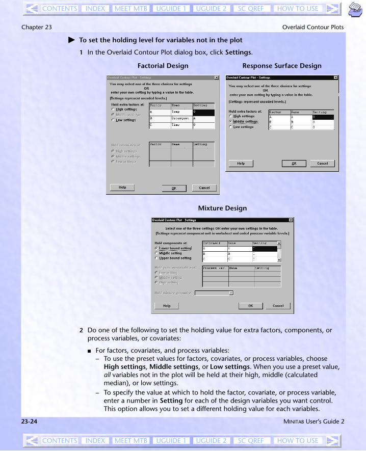
h To set the holding level for variables not in the plot
1 In the Overlaid Contour Plot dialog box, click Settings.
2 Do one of the following to set the holding value for extra factors, components, or process variables, or covariates:
■ For factors, covariates, and process variables:– To use the preset values for factors, covariates, or process variables, choose
High settings, Middle settings, or Low settings. When you use a preset value, all variables not in the plot will be held at their high, middle (calculated median), or low settings.
– To specify the value at which to hold the factor, covariate, or process variable, enter a number in Setting for each of the design variables you want control. This option allows you to set a different holding value for each variables.
Factorial Design Response Surface Design
Mixture Design
23-24 MINITAB User’s Guide 2
MEET MTB UGUIDE 1 SC QREFUGUIDE 2INDEXCONTENTS HOW TO USE

Overlaid Contour Plots Response Optimization
MEET MTB UGUIDE 1 SC QREFUGUIDE 2INDEXCONTENTS HOW TO USE
DOMROPTI.MK5 Page 25 Friday, December 17, 1999 1:06 PM
■ For components:– To use the preset values for components, choose Lower bound setting,
Middle setting, or Upper bound setting under Hold components at. When you use a preset value, all components not in the plot will be held at their lower bound, middle, or upper bound.
– To specify the value at which to hold the components, enter a number in Setting for each component that you want control. This option allows you to set a different holding value for each components.
3 Click OK.
e Example of an overlaid contour plot for factorial design
This contour plot is a continuation of the factorial response optimization example on page 23-13. A chemical engineer conducted a 23 full factorial design to examine the effects of reaction time, reaction temperature, and type of catalyst on the yield and cost of the process. The goal is to maximize yield and minimize cost. In this example, you will create contour plots using time and temperature as the two axes in the plot and holding type of catalyst at levels A and B respectively.
Step 1: Display the overlaid contour plot for Catalyst A
1 Open the worksheet FACTOPT.MTW. (The design information and response data have been saved for you.)
2 Choose Stat ➤ DOE ➤ Factorial ➤ Overlaid Contour Plots.
3 Click to move Yield and Cost to Selected.
4 Click Contours. Complete the Low and High columns of the table as shown below, then click OK in each dialog box.
Step 2: Display the overlaid contour plot for Catalyst B
5 Repeat steps 2-4, then click Settings. Under Hold extra factors at, choose High settings. Click OK in each dialog box.
Name Low HighYield 35 45
Cost 28 35
MINITAB User’s Guide 2 23-25
MEET MTB UGUIDE 1 SC QREFUGUIDE 2INDEXCONTENTS HOW TO USE
Chapter 23 Overlaid Contour Plots
MEET MTB UGUIDE 1 SC QREFUGUIDE 2INDEXCONTENTS HOW TO USE
DOMROPTI.MK5 Page 26 Friday, December 17, 1999 1:06 PM
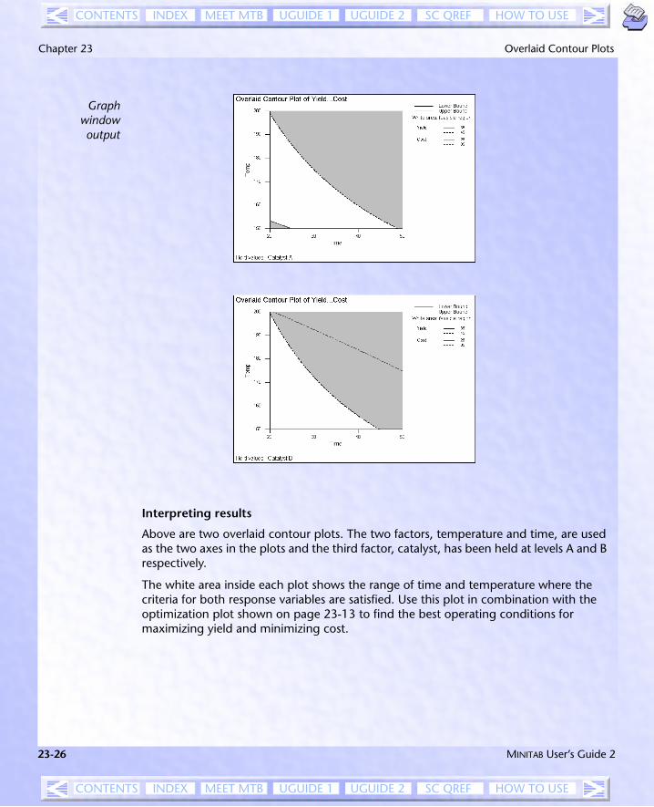
Interpreting results
Above are two overlaid contour plots. The two factors, temperature and time, are used as the two axes in the plots and the third factor, catalyst, has been held at levels A and B respectively.
The white area inside each plot shows the range of time and temperature where the criteria for both response variables are satisfied. Use this plot in combination with the optimization plot shown on page 23-13 to find the best operating conditions for maximizing yield and minimizing cost.
Graphwindowoutput
23-26 MINITAB User’s Guide 2
MEET MTB UGUIDE 1 SC QREFUGUIDE 2INDEXCONTENTS HOW TO USE
Overlaid Contour Plots Response Optimization
MEET MTB UGUIDE 1 SC QREFUGUIDE 2INDEXCONTENTS HOW TO USE
DOMROPTI.MK5 Page 27 Friday, December 17, 1999 1:06 PM
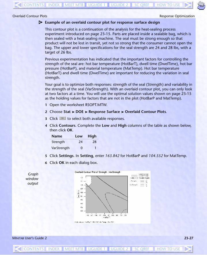
e Example of an overlaid contour plot for response surface design
This contour plot is a continuation of the analysis for the heat-sealing process experiment introduced on page 23-15. Parts are placed inside a sealable bag, which is then sealed with a heat-sealing machine. The seal must be strong enough so that product will not be lost in transit, yet not so strong that the consumer cannot open the bag. The upper and lower specifications for the seal strength are 24 and 28 lbs, with a target of 26 lbs.
Previous experimentation has indicated that the important factors for controlling the strength of the seal are: hot bar temperature (HotBarT), dwell time (DwelTime), hot bar pressure (HotBarP), and material temperature (MatTemp). Hot bar temperature (HotBarT) and dwell time (DwelTime) are important for reducing the variation in seal strength.
Your goal is to optimize both responses: strength of the seal (Strength) and variability in the strength of the seal (VarStrength). With an overlaid contour plot, you can only look at two factors at a time. You will use the optimal solution values shown on page 23-15 as the holding values for factors that are not in the plot (HotBarP and MatTemp).
1 Open the worksheet RSOPT.MTW.
2 Choose Stat ➤ DOE ➤ Response Surface ➤ Overlaid Contour Plots.
3 Click to select both available responses.
4 Click Contours. Complete the Low and High columns of the table as shown below, then click OK.
5 Click Settings. In Setting, enter 163.842 for HotBarP and 104.552 for MatTemp.
6 Click OK in each dialog box.
Name Low HighStrength 24 28
VarStrength 0 1
Graphwindowoutput
MINITAB User’s Guide 2 23-27
MEET MTB UGUIDE 1 SC QREFUGUIDE 2INDEXCONTENTS HOW TO USE
Chapter 23 Overlaid Contour Plots
MEET MTB UGUIDE 1 SC QREFUGUIDE 2INDEXCONTENTS HOW TO USE
DOMROPTI.MK5 Page 28 Friday, December 17, 1999 1:06 PM
Interpreting the results
The white area in the upper left corner of the plot shows the range of HotBarT and DwellTime where the criteria for both response variables are satisfied. You may increase of decrease the holding value to see the range change. To understand the feasible region formed by the three factors, you should repeat the process to obtain plots for all pairs of factors.
You can use the plots in combination with the optimizatopm plot shown on page 23-15 to find the best operating conditions for sealing the bags.
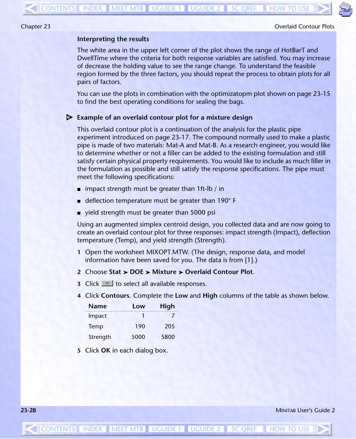
e Example of an overlaid contour plot for a mixture design
This overlaid contour plot is a continuation of the analysis for the plastic pipe experiment introduced on page 23-17. The compound normally used to make a plastic pipe is made of two materials: Mat-A and Mat-B. As a research engineer, you would like to determine whether or not a filler can be added to the existing formulation and still satisfy certain physical property requirements. You would like to include as much filler in the formulation as possible and still satisfy the response specifications. The pipe must meet the following specifications:
■ impact strength must be greater than 1ft-lb / in
■ deflection temperature must be greater than 190° F
■ yield strength must be greater than 5000 psi
Using an augmented simplex centroid design, you collected data and are now going to create an overlaid contour plot for three responses: impact strength (Impact), deflection temperature (Temp), and yield strength (Strength).
1 Open the worksheet MIXOPT.MTW. (The design, response data, and model information have been saved for you. The data is from [1].)
2 Choose Stat ➤ DOE ➤ Mixture ➤ Overlaid Contour Plot.
3 Click to select all available responses.
4 Click Contours. Complete the Low and High columns of the table as shown below.
5 Click OK in each dialog box.
Name Low HighImpact 1 7
Temp 190 205
Strength 5000 5800
23-28 MINITAB User’s Guide 2
MEET MTB UGUIDE 1 SC QREFUGUIDE 2INDEXCONTENTS HOW TO USE

References Response Optimization
MEET MTB UGUIDE 1 SC QREFUGUIDE 2INDEXCONTENTS HOW TO USE
DOMROPTI.MK5 Page 29 Friday, December 17, 1999 1:06 PM
Interpreting the results
The white area in the center of the plot shows the range of the three components, Mat-A, Mat-B, and Filler, where the criteria for all three response variables are satisfied.
You can use this plot in combination with the optimization plot shown on page 23-18 to find the “best” formulation for plastic pipe.
References[1] Koons, G. F. and Wilt, M. H. (1985). " Design and Analysis of an ABS Pipe
Compound Experiment", Experiments in Industry: Design, Analysis, and Interpretation of Results, edited by R.D. Snee, L.B.Hare, and R. Trout, American Society for Quality Control, Milwaukee, 111-117. zzz verify format
[2] Derringer, G. and Suich, R. (1980). Simultaneous Optimization of Several Response Variables, Jounral of Quality Technology, 12, 214-219.
[3] Myers, R.H. and Montgomery D.C. (1995). Response Surface Methodology. John Wiley & Sons, New York.
[4] Castillo, E.D., Montgomery, D.C., and McCarville, D.R. (1996). Modified Desirability Functions for Multiple Repsonse Optimization. Journal of Quality Technology, 28, 337-345.
Graphwindowoutput
MINITAB User’s Guide 2 23-29
MEET MTB UGUIDE 1 SC QREFUGUIDE 2INDEXCONTENTS HOW TO USE

Chapter 23 References
MEET MTB UGUIDE 1 SC QREFUGUIDE 2INDEXCONTENTS HOW TO USE
DOMROPTI.MK5 Page 30 Friday, December 17, 1999 1:06 PM
23-30 MINITAB User’s Guide 2
MEET MTB UGUIDE 1 SC QREFUGUIDE 2INDEXCONTENTS HOW TO USE