20200828 methodology report ecotransit world infras iml
TRANSCRIPT

EcoTransIT World
Environmental Methodology and Data
Update 2020
commissioned by
EcoTransIT World Initiative (EWI)

Document writing
Version Date Writer Modification
1.0 28.08.2020 R. Anthes Document creation
2.0 31.05.2021 R. Anthes, B. Notter, K.
Biemann, K. Dobers, other
Methodology Update 2020
General Contact
Ingenieurgesellschaft für Verkehrs- und Eisenbahnwesen mbH
Consulting Company for Traffic and Railway Engineering Ltd.
Lützerodestr. 10, 30161 Hannover, Germany
Project Manager:
Dipl.-Ing. Ralph Anthes | Dr.-Ing. Alena Schmidt
+49 511 897668-18 | +49 511 897668-19
+49 511 897668-10 (Secretariat)

In Cooperation with
Infras AG – Consulting, Analysis and Research
Berne, Switzerland
Ifeu – Institut für Energie- und Umweltforschung
Heidelberg, Germany
Fraunhofer Institute for Material Flow and Logistics IML
Dortmund, Germany
Responsibilities
Topic Contact Contact Address
Truck, Train, Energy Supply Kirsten Biemann, ifeu
Wolfram Knörr, ifeu
Christoph Heidt, ifeu
Sea ship Benedikt Notter, INFRAS [email protected]
Inland ship Benedikt Notter, INFRAS
Christoph Heidt, ifeu
Aircraft Hans-Jörg Althaus, INFRAS [email protected]
Logistic Sites Kerstin Dobers, Fraunhofer IML [email protected]
Business Solutions,
Routing, GIS-Data,
Ralph Anthes, IVE
Alena Schmidt, IVE
alena.schmidt@ivembh,de

Table of contents
Document writing ....................................................................................................................... 1
General Contact ........................................................................................................................... 1
Table of contents ......................................................................................................................... 3
Foreword ....................................................................................................................................... 1
1 Introduction .......................................................................................................................... 2
1.1 Background and task .......................................................................................................................... 2
1.2 Accordance with EN 16258 ............................................................................................................. 3
1.3 Accredited to be compliant with the GLEC Framework .................................................... 6
2 ETW business solutions ..................................................................................................... 7
2.1 Additional features compared to the website http://ecotransit.org .......................... 7
2.1.1 Methodology support included .............................................................................................. 8
2.2 Available Interfaces (API) ............................................................................................................. 10
2.2.1 SOAP XML Webservice ............................................................................................................ 10
2.2.2 CSV File Mass Calculation...................................................................................................... 10
2.2.3 ETW on Customer Website ................................................................................................... 11
2.3 Calculation Service ........................................................................................................................... 11
3 System boundaries and basic definitions .................................................................. 12
3.1 Transport service and vehicle operation system .............................................................. 12
3.2 Environmental impacts .................................................................................................................. 13
3.3 System boundaries of processes ................................................................................................ 15
3.3.1 Environmental relevance of excluded processes ......................................................... 16
3.4 Transport modes and propulsion systems ........................................................................... 19
3.5 Spatial differentiation ..................................................................................................................... 19
3.5.1 Road and rail .............................................................................................................................. 19
3.5.2 Sea and inland ship .................................................................................................................. 20
4 Basic definitions and calculation rules ...................................................................... 23
4.1 Main factors of influence on energy and emissions of freight transport ............... 23
4.2 Logistics parameters ....................................................................................................................... 24
4.2.1 Definition of payload capacity ............................................................................................ 25
4.2.2 Definition of capacity utilisation ........................................................................................ 30
4.2.3 Capacity Utilisation for specific cargo types and transport modes..................... 31
4.3 Basic calculation rules .................................................................................................................... 38
4.3.1 Final energy consumption per net tonne km (TTW) ................................................. 38

4.3.2 Energy related emissions per net tonne km (TTW) ................................................... 40
4.3.3 Combustion related emissions per net tonne km (TTW) ......................................... 41
4.3.4 Upstream energy consumption and emissions per net tonne km (WTT) ......... 41
4.3.5 Total energy consumption and emissions of transport (WTW) ........................... 42
4.4 Basic allocation rules....................................................................................................................... 43
5 Routing of transports ...................................................................................................... 46
5.1 General ................................................................................................................................................... 46
5.2 Routing with resistances ............................................................................................................... 46
5.2.1 Road network resistances ..................................................................................................... 47
5.2.2 Railway network resistances ............................................................................................... 47
5.3 Sea ship routing ................................................................................................................................. 48
5.3.1 Routing inland waterway ship ............................................................................................ 50
5.4 Aviation routing ................................................................................................................................. 50
5.5 Determination of transport points within combined transport chains .................. 51
5.5.1 Definition of side tracks for rail transports ................................................................... 52
6 Methodology and environmental data for each transport mode ........................ 54
6.1 Road transport ................................................................................................................................... 54
6.1.1 Classification of truck types.................................................................................................. 54
6.1.2 Final energy consumption and vehicle emission factors (TTW) .......................... 55
6.1.3 Final energy consumption and vehicle emissions (TTW) ........................................ 60
6.1.4 Alternative fuel trucks ............................................................................................................ 63
6.2 Rail transport ...................................................................................................................................... 67
6.2.1 Train Types .................................................................................................................................. 67
6.2.4 Final energy consumption (TTW) ...................................................................................... 68
6.2.5 Energy consumption of diesel trains ................................................................................ 73
6.2.6 Shunting ........................................................................................................................................ 77
6.3 Sea transport ....................................................................................................................................... 78
6.3.1 Overview ....................................................................................................................................... 78
6.3.2 Derivation of basic fuel consumption and emission factors ................................... 78
6.3.3 Aggregation to ETW size classes and trade lanes ...................................................... 82
6.3.4 Adjustments for speed and cargo utilization ................................................................ 86
6.3.5 Consideration of emission control areas (ECAs) ......................................................... 89
6.3.6 Allocation rules for seaborne transport .......................................................................... 91
6.3.7 Ferry transport .......................................................................................................................... 91
6.4 Inland waterway transport .......................................................................................................... 93
6.4.1 Overview ....................................................................................................................................... 93

6.4.2 Inland waterways in ETW ..................................................................................................... 94
6.4.3 Derivation of basic fuel consumption and emission factors ................................... 96
6.4.4 Allocation rules for inland waterway transport ......................................................... 98
6.5 Air transport ........................................................................................................................................ 98
6.5.1 Type of airplanes and load factor ...................................................................................... 98
6.5.2 Energy consumption and emission factors (Tank-to-Wheel) .............................. 101
6.5.3 Emission Weighting Factor (EWF).................................................................................. 105
6.5.4 Allocation method for belly freight ................................................................................. 106
6.6 Energy consumption and emissions of the upstream process (WTT) ................. 108
6.6.1 Exploration, extraction, transport and production of liquid fuels..................... 109
6.6.2 Electricity production ........................................................................................................... 110
6.7 Biofuel shares .................................................................................................................................. 114
6.8 Cooled transports .......................................................................................................................... 117
7 Appendix ........................................................................................................................... 121
7.1 EN 16258: Default conversion factors ................................................................................. 121
7.2 Example for an ETW declaration in accordance with EN 16258 ............................ 122
7.3 Additional information to load factors ................................................................................ 122
7.3.1 Train ............................................................................................................................................. 123
7.3.2 Container .................................................................................................................................... 123
7.4 Detailed data of aircrafts included in EcoTransIT ......................................................... 126
8 References ........................................................................................................................ 127
8.1 General ................................................................................................................................................ 127
8.2 Road transport ................................................................................................................................ 128
8.3 Rail transport ................................................................................................................................... 129
8.4 Inland ship and Marine transport .......................................................................................... 129
8.5 Ferries.................................................................................................................................................. 130
8.6 Aircraft transport ........................................................................................................................... 131
8.7 Energy supply and biofuel shares .......................................................................................... 132
8.8 Cooled transports .......................................................................................................................... 132
9 Expressions and abbreviations .................................................................................. 134

EcoTransIT World - Methodology Report 1
Foreword
The EcoTransIT Initiative (EWI) is an independent industry driven platform for carriers,
logistics service providers and shippers dedicated to maintain and develop a globally
recognized tool and methodology for carbon footprints and environmental impact
assessments of the freight transport sector.
In line with its vision to increase transparency on the environmental impact of the
freight transport and to demonstrate the continuous improvement of EcoTransIT
methodology and EcoTransIT World (ETW) calculator, EWI members have
commissioned their scientific and IT partners to provide an updated methodology
report. The methodology was already embedded in the calculator; it follows the
guidelines of the standard EN 16258 “Methodology for calculation and declaration of
energy consumption and greenhouse gas emissions of transport services” and integrates
latest research available for the air pollutants.
There are over 40 companies’ member of the EWI. A complete EWI member and user list
can be found at the website https://ecotransit.org
These members also thank their scientific and IT partners - INFRAS Berne, ifeu
Heidelberg, Fraunhofer IML Dortmund and IVE Hannover - for their continuous support
to the vision of EWI.

EcoTransIT World - Methodology Report 2
1 Introduction
1.1 Background and task
As freight transport mainly relies on conventional energy carriers like diesel, kerosene
and heavy fuel oil, it significantly contributes to major challenges of the 21st century:
pollution and climate change. According to the Fifth Assessment Report from the
Intergovernmental Panel on Climate Change, transport accounts for about a quarter of
global energy-related carbon emissions. This contribution is rising faster than on any
other energy end-use sector.
EcoTransIT World means Ecological Transport Information Tool – worldwide (ETW). It
is a free of charge internet application, which shows the environmental impact of freight
transport – for any route in the world and any transport mode. More than showing the
impact of a single shipment, it analyses and compares different transport chains with each
other, thus making evident which solution has the lowest impact.
For professional users, ETW offers dedicated services that allow companies to calculate
large numbers of shipments at once without manual handling efforts. It provides a
customized interface based on individual customer’s operational data and answering its
needs and requirements. Thus, with ETW Business Solutions the corporate data
warehouse can be filled with all information required to realize specific environmental
reports, regional inventories, establish carbon reporting or provide carbon accounting
benchmarks efficiently.
With this purpose in mind, EcoTransIT World aims to address:
- Forwarding companies willing to reduce the environmental impact of their shipments;
- Carriers and logistic providers being confronted with growing requests from
customers as well as legislation to show their carbon footprint and improve their
logistical chains from an environmental perspective;
- Political decision makers, consumers and non-governmental organisations which are
interested in a thorough environmental comparison of logistic concepts including all
transport modes (lorry, railway, ship, airplane and combined transport).
The environmental parameters covered are energy consumption, carbon dioxide (CO2),
sum of all greenhouse gases (measured as CO2 equivalents) and air pollutants, such as

EcoTransIT World - Methodology Report 3
nitrogen oxides (NOx), sulphur dioxide (SO2), non-methane hydro carbons (NMHC) and
particulate matter (PM).
The online application offers two levels: In a “standard” input mode it allows a rough
estimate. This can be refined in an “extended” input mode according to the degree of
information available for the shipment. Thus, all relevant parameters like route
characteristics and distance, load factor and empty trips, vehicle size and engine type are
individually taken into account and can be changed by the user.
The initial version of EcoTransIT was published in 2003 with a regional scope limited to
Europe. The version published in 2010 was expanded to a global scope. For the first time,
EcoTransIT World (ETW) enabled the calculation of environmental impacts of worldwide
freight transport chains. For this purpose, the routing logistics of the tool as well as the
information about environmental impacts of all transport modes (in particular sea and
air transport) were expanded. In the meantime, the methodology was updated
considering new sources, data and knowledge. In this context the requirements of the new
European standard EN 16258: 2012 “Methodology for calculation and declaration of
energy consumption and greenhouse gas emissions of transport services” were also taken
into account.
Thus, ETW offers a ‘best-practice’ standard of carbon foot-printing and green accounting
to the whole sector – compliant with international standards like the European standard
EN 16258.
The internet version of ETW as well as the integrated route planner for all transport
modes has been realized by IVE Hannover. The methodology, input data and default
values for the ecological assessments of the transport chains are developed and
provided by ifeu Heidelberg, INFRAS Berne and Fraunhofer IML Dortmund. ifeu, INFRAS
and Fraunhofer IML ensure that the ETW methodology is always up-to-date and in
accordance with the international standards.
The present report “Methodology and Data Update” documents the methodology and the
data currently embedded in ETW.
1.2 Accordance with EN 16258
Since the very first beginning EcoTransIT World has been provided a harmonized,
independent methodology for the calculation of GHG emissions and air pollutants. The
overall methodology and the approaches for each transport mode were very similar to

EcoTransIT World - Methodology Report 4
the suggestion from the new European standard EN 16258 - which was published by the
British Standards Institution (BSI) as BS EN 16258, by the German Institute for
Standardisation (Deutsches Institut für Normung, DIN) as DIN EN 16258 and by
Association française de normalisation (AFNOR) as NF EN 16258 at the end of 2012.
Thus, the adaptation of the ETW methodology to the requirements of the European
standard was feasible. The calculation of energy consumption and greenhouse gas
(GHG) emissions (as CO2 equivalents) by ETW is fully in accordance with EN 16258.
One methodological principle of the new standard is that in a first step the final energy
consumption (litre Diesel, kWh electricity) of each part of the transport services (so-
called leg) have to be calculated and in a second step these values have to be transferred
into standardized energy consumption (MJ) and CO2 equivalent emissions (kg CO2e) on a
Tank-to-Wheels (TTW) and Well-to-Wheels (WTW) basis (see chapter 3.3). The new
standard contains the necessary conversion factors respectively default values for
these calculations (e.g. MJ/litre or kg CO2e/litre diesel). ETW uses the conversion factors
for fuels included in EN 16258 without changes (see chapter 7.1 in the annex of this
report). For electricity the standard EN 16258 does not contain conversion factors as
these are dependent on the mix of the generating plants which produced the electricity.
The European standard only includes general rules for calculation of conversion factors
for electricity. ETW uses own calculated conversion factors for electricity for trains
which are in line with these general requirements of EN 16258 (see chapter 6.6).
In accordance with EN 16258 the final energy consumptions, the load factor or share of
empty trips for the transport service can be measured or calculated by using default
values. In general, ETW uses only default values for the calculation of energy
consumption and GHG emissions since measured values can only be provided by the
users themselves. The default values used by ETW are based on well-established data
bases, statistical data and literature reviews. The data sources for default values
suggested by EN 16258 were considered. Therefore, ETW uses only default values being
in accordance with new European Standard.
Furthermore, ETW allows users to change vehicle sizes, emission standards, load factors
and shares of empty trips based on own data or measurements. In these cases, the user
of ETW has to be ensured that the used figures are in accordance with the European
standard. Fuel consumption figures as well as conversion factors can’t be changed by the
user. Fuel consumption data can only be replaced by business solutions of ETW after
evaluation by the scientific partners ifeu or INFRAS (see chapter 2).

EcoTransIT World - Methodology Report 5
In normal cases the goods considered with ETW do not fit exactly with the capacity of
the chosen vehicles, trains, vessels or airplanes so that the energy consumption or
emissions have to be allocated to the transport service considered. The European
standard recommends carrying out the allocation using the product of weight and
distance (e.g. tonne kilometres). Where this is not possible, then other physical units
(e.g. pallet spaces, loading meters, number of container spaces) can be used instead of
weight. ETW always uses the allocation unit tonne kilometres. Only for transport of
containers the allocation unit TEU kilometres (= twenty-foot equivalent unit) is
considered. The allocation methodologies used by ETW are also in accordance with the
European standard.
Furthermore, the European standard describes requirements for the declaration of the
results of the calculation: the declaration must disclose the well-to-wheels energy
consumption and greenhouse gas emissions as well as the tank-to-wheels energy
consumption and greenhouse gas emissions for the transport service considered. In
addition, the sources used for the distance, load utilisation, empty trip percentage and
energy consumption parameters must be identified. This report documents the default
values used for the calculations in ETW and delivers additional information for
declarations in accordance with EN 16258. Since the report is comprehensive and
detailed, ETW provides a short declaration which includes all important information
required (e.g. data sources used). The short declaration is provided by the ETW internet
tool for each calculation carried out by the user. One example of this brief declaration is
given in the annex of this report (see chapter 7.2).
Thus, the results for energy consumption and GHG emissions calculated with ETW
are in compliance with the standard EN 16258:2012.
Moreover, the European standard points out the following points, if the user wants to
compare results calculated with different tools: “Please consult this standard to get
further information about processes not taken into account, guidelines and general
principles. If you wish to make comparisons between these results and other results
calculated in accordance with this standard, please take particular care to review the
detailed methods used, especially allocation methods and data sources.
"Last but not least” it has to be mentioned that one of the triggers for the European
standard was that France planned to legalize oblige transport operators to show their
customers the CO2 emissions produced by the transport service. However, it was not
clear which methods should be used for determining the emissions. For this reason, in

EcoTransIT World - Methodology Report 6
2008 France made a standardisation application to the European Committee for
Standardisation (CEN).
In the interim the French Decree No. 2011-1336 on "Information on the quantity of
carbon dioxide emitted during transport" was published and updated in 2017. It
stipulates that, by 1st of October 2013 at the latest, CO2e values of commercial passenger
and freight transport which begin or end in France must be declared to the customer.
This decree basically uses the same methodology as the European standard. However,
there are also significant differences from the standard EN 16258. Furthermore, the
French decree use different conversion factors compared to the EN 16258. They are not
comparable so it is not possible to use the conversion factors of the European standard
and the French decree at the same time. The ETW internet tool provides only results
based on the conversion factors based on EN 16258. But in ETW business solutions the
conversion factors included in the French decree can also be used so that ETW can also
provide results in accordance with the French decree (see chapter 2).
1.3 Accredited to be compliant with the GLEC Framework
EcoTransIT World is the first emission calculation tool which is accredited to be compliant
with the global GLEC framework. The Global Logistics Emissions Council (GLEC)
framework established by Smart Freight Centre (SFC) has been created to be the leading
methodology for freight transports and logistics operations. It allows companies to
consistently calculate their GHG footprint across the global multi-modal supply chain.
As part of the accreditation statement SFC confirmed the ETW calculation to be in line
with Well-to-Wheel GHG emissions according the scopes of the GHG Protocol Corporate
Value Chain Accounting and Reporting Standard.

EcoTransIT World - Methodology Report 7
2 ETW business solutions
The ETW Business Solutions contain standardised interfaces (API) for automatic emission
calculation of huge amounts of transport chains. Already today, several hundred million
transports are calculated every year via the API. The use ranges from an individualised
website to semi-automatic calculations of transport lists in CSV format to a fully automatic
solution based on a SOAP XML Webservice (WSDL).
The ready-to-use standard solutions are extremely flexible and allow to calculate complex
intermodal transport chains with little or much customer-specific transport information.
If necessary, user-defined adaptations or extensions to the software are made available.
The interfaces are offered as Software-as-a-Service. The associated servers are provided
by IVE mbH and are continuously monitored by specific monitoring software. Server costs
and regular updates are included in the license fees. In addition to the API, the IVE mbH
team offers to calculate, analyse and present customer-specific transports as consultation
projects.
2.1 Additional features compared to the website
http://ecotransit.org
The ETW Business Solution enables valuable additional features which are not available
on the global website of ETW. These features are:
- Automated calculation of large transport volumes
- Individual technical and methodical consultation
- Consideration of customer-specific transport characteristics
- Calculation of container sea shipments via the Clean Cargo
Working Group (CCWG) methodology, including
o calculation of EC, GHG emissions and SOx based on
CCWG trade lane emission factors
o adjustable allocation factor (default 70%) and
flexible distance correction factor (default 15%)
o sophisticated trade lane mapping
o usage of SCAC based emission factors (only for CCWG members)
- Automatically flight number analyses via OAG.com interface:
o enables appliance of an aircraft share via flight

EcoTransIT World - Methodology Report 8
number, flight carrier or airport pair (inclusive belly or freighter detection)
o optional stop-over identification
- Additional vehicle classes, like over 250 different plane types or additional truck and
train classes
- Calculation of logistics sites emissions for e.g. warehouse or transhipment
processes via the REff Tool® (https://reff.iml.fraunhofer.de/) and
Fraunhofer IML’s methodology1
- Calculation with Twenty-foot Equivalent (TEU) and Forty-foot Equivalent (FEU)
containers
- Automatically conversion of the truck load to the respective load factor (FTL, LTL,
FCL) including the usage of the respective vehicle type
- Consideration of individual transport distances per leg for all transport types
- Output split per country or vehicle type (can be used e.g. for result manipulation
forward to the French decree)
- LocationEditor: Inclusion and correction of new or customer-specific locations
- LogViewer: Create statistics and analyses of the calculated results
- Data security provided by dedicated hardware with secured encrypted data transfer
- Participating within the EWI to initiate new working groups, methodology issues and
help to steer ETW
All features can be adjusted or enlarged on individual basis towards to the company own
needs.
2.1.1 Methodology support included
All ETW Business Solutions include a consulting package which automatically enables
methodology support done by our scientific partners.
1 The ETW Business Solutions provides the possibility of assessing the environmental
impact of logistics sites’ operations on the basis of company’s real data. Logistics sites play
a connecting role within transport chains and refer to all sites that combine different
transport legs (within and between modes) or are the starting or end point of transport
chains. The assessment scope follows the methodology as described in /Fraunhofer IML
2019/.

EcoTransIT World - Methodology Report 9
In principle almost, every development/ adjustment to the customers’ needs can be done
within the ETW Business Solutions. The effort for such an individual solution depends on
the respective specification.

EcoTransIT World - Methodology Report 10
2.2 Available Interfaces (API)
The ETW Business Solutions contain standardised interfaces (API) for automatic mission
calculation of huge amounts of transport chains. Already today, several hundred million
transports are calculated every year via the API. The use ranges from an individualised
website to semi-automatic calculations of transport lists in CSV format to a fully automatic
solution based on a Soap XML Web Service (WSDL). The ready-to-use standard solutions
are extremely flexible and allow to calculate complex intermodal transport chains with
little or much customer-specific transport information. If necessary, user-defined
adaptations or extensions to the software are made available.
The interfaces are offered as Software-as-a-Service. The associated servers are provided
by IVE mbH and are continuously monitored by specific monitoring software. Server
costs and regular updates are included in the license fees.
Figure 1 Different kinds of standardized interfaces
2.2.1 SOAP XML Webservice
The SOAP XML Webservice enables the calculation of single requests on the base of a
WSDL web service. The request can include all modes including an unlimited amount of
via points on base of the ETW characteristics. The SOAP XML webservice includes several
request types, like calculation requests, flight number requests, location and vehicle
requests and many more. Due to these request types it is possible to create a complete
external calculation website which uses only SOAP XML requests/ responses.
2.2.2 CSV File Mass Calculation
Within the interface of the CSV File Mass Calculation the user can upload request files
including huge numbers of transport services and download response files (csv, pdf, kml
or rtf) including calculation results. Within the so-called mass calculation every transport

EcoTransIT World - Methodology Report 11
service will be calculated separately. The upload and download can be done via a login
and password secured website or via a sFTP interface.
2.2.3 ETW on Customer Website
ETW can be included on customers’ websites. The integration can be realized via a so
called iframe or by the customer IT itself by using the SOAP XML Webservice.
2.3 Calculation Service
In addition to the API, the IVE mbH team offers to calculate, analyse and present customer-
specific transports as consultation projects. Already now several shipper companies using
this service of IVE to calculate their shipments on detailed level.

EcoTransIT World - Methodology Report 12
3 System boundaries and basic definitions
The following subchapters give an overview about the system boundaries and definitions
used in ETW. In comparison to the European standard EN 16258 “Methodology for
calculation and declaration of energy consumption and greenhouse gas emissions of
transport services” ETW allows also the quantification of other emissions like air
pollutants for transport chains. Nevertheless, ETW considers all requirements of EN
16258 independent of the environmental impact category considered. The system
boundaries as well as definitions are chosen in such a way that they are in accordance
with the new European standard.
3.1 Transport service and vehicle operation system
ETW allows the calculation of different environmental impact categories (see next
subchapter) for a single transport from A to B or for complex transport chains using
different transport modes. In the context of the European standard EN 16258 these
transport cases are called transport services. According to EN 16258 a transport service
is a “service provided to a beneficiary for the transport of a cargo […] from a departure
point to a destination point”. The EN 16258 methodology requires that the transport
service has to be broken down into sections in which the cargo considered travels on a
specified vehicle, i.e. without changing vehicle. This section of route is also called leg in
the standard. The level of energy consumption and emissions for the consignment under
consideration must be determined for each leg and then added to give an overall result.
ETW works exactly in this way. For each leg the quantification is done separately and the
overall sum is calculated for the entire transport service. Therefore, ETW fulfils these
requirements of EN 16258.
Additionally, EN 16258 demands that energy consumption and the GHG emissions for
each leg have to be quantified using the so-called Vehicle Operation System (VOS). VOS is
the term which the standard uses to denote the round-trip of a vehicle in which the item
in question is transported for a section of the route. The VOS does not necessarily have to
be an actual vehicle round-trip. It can also consist of all vehicle round-trips for one type
of vehicle or of one route or leg or even of all vehicle round-trips in a network in which
the transport section in question lies or would lie (for future transport services). In the
end the energy consumption for the entire VOS needs to be determined and then allocated
to the transport leg and the individual consignment under consideration.

EcoTransIT World - Methodology Report 13
In accordance with EN 16258 the energy consumption of a VOS can be measured or be
calculated by using default values. As mentioned in chapter 1.2 the internet tool of ETW
only uses default values particularly for energy consumption of trucks, trains, ships and
airplanes. Therefore, the VOS established for the calculation for ETW is the entire round
trip of these vehicles or vessels. To consider the energy consumption for a single transport
service the fuel or electricity consumption of the vehicles or vessels are allocated to the
shipment by using the units’ tonne kilometres or TEU kilometres. The transport distance
is calculated by the integrated route planner of ETW (see chapter 5). The weight of the
shipment or the number of TEU is calculated by using the maximum payload capacity, the
load factor and share of additional empty trips (see chapter 4.2). Similar to energy
consumption ETW considers the load factor and additional share of empty trips for the
entire VOS. Thus, the ETW definition of VOS fulfils all requirements of the EN 16258.
However, it must be noted that specific energy consumption values per tonne kilometre
or TEU kilometre used in ETW already take account of the load factors and empty trips
and link the energy consumption calculation directly to the allocation step – so, instead of
two separate steps mentioned in the EN 16258 (calculation of energy consumption and
afterwards allocation to the single shipment), ETW combine both steps. But the results
are identical independent of combining the two steps or not.
3.2 Environmental impacts
Transportation has various impacts on the environment. These have been primarily
analysed by means of life cycle analysis (LCA). An extensive investigation of all kinds of
environmental impacts has been outlined in /Borken 1999/. The following categories
were determined:
- Resource consumption
- Land use
- Greenhouse effect
- Depletion of the ozone layer
- Acidification
- Eutrophication
- Eco-toxicity (toxic effects on ecosystems)
- Human toxicity (toxic effects on humans)
- Summer smog
- Noise

EcoTransIT World - Methodology Report 14
The transportation of freight has impacts within all these categories. However, only for
some of these categories it is possible to make a comparison of individual transport
services on a quantitative basis. Therefore, in ETW the selection of environmental
performance values had to be limited to a few but important parameters. The selection
was made according to the following criteria:
- Particular relevance of the impact
- Proportional significance of cargo transports compared to overall impacts
- Data availability
- Methodological suitability for a quantitative comparison of individual transports.

EcoTransIT World - Methodology Report 15
The following parameters for environmental impacts of transports were selected:
Table 1 Environmental impacts included in EcoTransIT World
Abbr. Description Reasons for inclusion
PEC Primary energy consumption Main indicator for resource consumption CO2 Carbon dioxide emissions Main indicator for greenhouse effect
CO2e Greenhouse gas emissions as CO2-equivalent. CO2e is calculated as follows (mass weighted): CO2e = CO2 + 25 * CH4 + 298 * N2O CH4: Methane N2O: Nitrous Oxide
Greenhouse effect
NOx Nitrogen oxide emissions Acidification, eutrophication, eco-toxicity, human toxicity, summer smog
SO2 Sulphur dioxide emissions Acidification, eco-toxicity, human toxicity NMHC Non-methane hydro carbons Human toxicity, summer smog
Particles Exhaust particulate matter from vehicles and from energy production and provision (power plants, refineries, sea transport of primary energy carriers), in ETW particles are quantified as PM 10
Human toxicity, summer smog
Thus, the categories land use, noise and depletion of the ozone layer were not taken
into consideration. In reference to electricity-driven rail transport, the risks of nuclear
power generation from radiation and waste disposal were also not considered. PM
emissions are defined as exhaust emissions from combustion; therefore, PM emissions
from abrasion and twirling are also not included in ETW.
In accordance with EN 16258 energy consumption and GHG emissions measured as CO2
equivalents can be calculated with ETW. The definitions used by ETW are similar to the
definitions of EN 16258.
3.3 System boundaries of processes
In ETW, only environmental impacts linked to the operation of vehicles and to fuel or
energy production are considered. Therefore, the following are not included:
- The production and maintenance of vehicles;
- The construction and maintenance of transport infrastructure;
- Additional resource consumption like administration buildings, stations, airports,
etc...
All emissions directly caused by the operation of vehicles and the final energy
consumption are taken into account. Additionally, all emissions and the energy

EcoTransIT World - Methodology Report 16
consumption of the generation of final energy (fuels electricity) are included. The
following figure shows an overview of the system boundaries.
Figure 2 System boundaries of processes /own figure adapted from Geodis/
In ETW, two process steps and the sum of both are distinguished:
- Final energy consumption and vehicle emissions (= operation; Tank-to-Wheels TTW),
- Upstream energy consumption and upstream emissions (= energy provision,
production and distribution; Well-to-Tank WTT),
- Total energy consumption and total emissions: Sum of operation and upstream figures
(Well-to-Wheels WTW).
The new European standard EN 16258 requires the calculation and declaration of energy
consumption and GHG emissions of transport services on TTW as well as WTW basis.
ETW provides both figures for energy consumption and GHG emissions. In this context
attention should be paid to fact that WTW energy consumption is also very often referred
to as primary energy consumption, TTW energy consumption as final energy
consumption.
3.3.1 Environmental relevance of excluded processes
The EN 16258 follows a Well-to- wheels approach and thus does not include the transport
infrastructure (streets, railways,…) and the vehicles used for transport (e.g.
manufacturing, maintenance and end-of-life for trucks, airplanes, trains and ships).

EcoTransIT World - Methodology Report 17
In this chapter a short information on the relevance for these processes for the entire
process chain is given.
A recently published study for the Umweltbundesamt (ifeu/ infras/ Öko Institut 2020)
shows that the relevance of the vehicle and the infrastructure differs between the
different transport modes, vehicle sizes and environmental impact categories.
In general, greenhouse gas emissions today as well as emissions of air pollutants are
dominated by the well-to-wheels emissions. For the GHG emissions, the infrastructure
contributes only marginally to the overall impacts. Vehicles are also almost irrelevant for
air, train or ship and have a very low impact for trucks. The nitrous oxide emissions show
a slightly bigger, but still very small, contribution from infrastructure and vehicles to the
overall process chain.
Figure 3 Comparison of the GHG emissions from road transportation in Germany in 2017 in g per tkm [ifeu/ infras/ Öko Institut 2020]
*Vehicles includes production, maintenance and end-of-life
** For aircrafts, the additional climate impacts of emissions at high altitudes are included by using an emission weighting
factor (EWF). More details on these effects can be found in chapter 6.5.3.
More relevant are the contributions from the particulate emissions. In recent years, direct
particulate emissions at the vehicle exhaust level have decreased greatly, leading to a
higher contribution of the WTT part of the process chain and the emissions from vehicles
and infrastructure.
Today most vehicles are driven using fossil fuels. In the future this picture may however
be changing. The introduction of electric vehicles leads to an increase of the emissions
from vehicle manufacturing due to the high impacts from the lithium ion battery. Electric
0 200 400 600 800 1000 1200 1400
rigid truck 3,5-7,5t
rigid truck >7,5-12t
rigid truck >12t
articulated lorry >34-40t
rail freight transport
inland waterway shipping
aircraft (international)
g CO2e/ tkm
energy supply (WTT) use phase (TTW) vehicles infrastructure EWF

EcoTransIT World - Methodology Report 18
trucks have no direct greenhouse gas or air pollutant emissions, but the provision of the
electricity today leads to still considerable impacts in most countries worldwide.
These impacts will likely decrease in the future when more renewable energy is used for
electricity generation.
A study done by Ricardo, ifeu and e4tech for the European Commission [Ricardo, ifeu,
e4tech 2020] concludes that the battery manufacturing of lithium ion batteries today lead
to greenhouse gas emissions of around 80 kg CO2e per kWh battery capacity. Even though
the emissions from the vehicle provision increase compared to the conventional truck,
when using an average European electricity mix, a battery electric truck with 12 t GVW
has almost half the GHG emissions compared to a diesel truck.
Figure 4 Comparison of the GHG emissions for a 12 t GVW truck in 2020 with EU electricity mix [Ricardo, ifeu, e4tech 2020]
This assessment shows that even though the emissions from vehicle manufacturing are
increasing for alternatively fueled vehicles, GHG emissions are still dominated by the
WTW part of the process chain.
0 50 100 150 200 250 300 350 400
rigid truck >7,5-12t diesel
rigid truck >7,5-12t BEV
g CO2e/ tkm
WTT TTW vehicle production Maintenance end-of-life

EcoTransIT World - Methodology Report 19
3.4 Transport modes and propulsion systems
Transportation of freight is performed by different transport modes. Within ETW, the
most important modes using common vehicle types and propulsion systems are
considered. They are listed in the following table.
Table 2 Transport modes, vehicles and propulsion systems
Transport mode Vehicles/Vessels Propulsion energy
Road Road transport with single trucks and truck
trailers/articulated trucks (different types) Diesel fuel, CNG, LNG, Electricity
Rail Rail transport with trains of different total
gross tonne weight
Electricity and diesel fuel
Inland waterways Inland ships (different types) Diesel fuel
Sea Ocean-going sea ships (different types)
and ferries
Heavy fuel oil (HFO) / marine diesel oil
(MDO) / marine gas oil (MGO)
Aircraft transport Air planes (different types) Kerosene
3.5 Spatial differentiation
In ETW worldwide transports are considered. Therefore, environmental impacts of
transport can vary from country to country due to country-specific regulations, energy
conversion systems (e.g. energy carrier for electricity production), traffic infrastructure
(e.g. share of motorways and electric rail tracks) and topography.
Special conditions are also relevant for international transports by sea ships. Therefore, a
spatial differentiation is necessary. For sea transport, a distinction is made for different
trade lanes and areas (Sulphur Emission Control Areas/SECA). On the contrary, for
aircraft transport, the conditions relevant for the environmental impact assessments are
similar all over the world.
3.5.1 Road and rail
For road and rail transport, ETW distinguishes between Europe and other countries. In
this version of ETW, it was not possible to find accurate values for the transport systems
of each country worldwide. For this reason, we defined seven world regions and within
each region, we identified the most important countries with high transport performance
and considered each one individually. For all other countries within a region, we defined
default values, normally derived from an important country of this region. In further

EcoTransIT World - Methodology Report 20
versions, the differentiation can be refined without changing the basic structure of the
model. The following table shows the regions and countries used.
Table 3 Differentiation of regions and countries for road and rail transport
Significant influencing factors are the types of vehicles used, the type of energy, the share
of biofuel blends and the conversion factors used. Wide variations result particularly from
the national mix of electricity production.
Differences may exist for railway transport, where the various railway companies employ
different locomotives and train configurations. However, the observed differences in the
average energy consumption are not significant enough to be established statistically with
certainty. Furthermore, within the scope of ETW, it was not possible to determine specific
values for railway transport for each country. Therefore, a country specific differentiation
of the specific energy consumption of cargo trains was not carried out.
3.5.2 Sea and inland ship
For ocean-going vessels, a different approach was taken because of the international
nature of their activity. The emissions for sea ships were derived from the Third IMO
Greenhouse Gas Study /IMO 2015/. For each intercontinental (e.g. North America to
Europe) or major inter-regional (North-America to South-America) trade lane the
common size of deployed ships was analysed, using schedules from ocean carriers. The
trade lane-specific emission factors were aggregated from IMO ship types and size classes
using the trade lane-specific vessel sizes. Figure 3 shows the connected world regions and
ID Region Country Code ID Region Country Code
101 Africa default afr 514 Europe Iceland IS102 Africa South Africa ZA 515 Europe Ireland IE201 Asia and Pacific default asp 516 Europe Israel IL202 Asia and Pacific China CN 517 Europe Italy IT203 Asia and Pacific Hong Kong HK 518 Europe Latvia LV204 Asia and Pacific India IN 519 Europe Lithuania LT205 Asia and Pacific Japan JP 520 Europe Luxembourg LU206 Asia and Pacific South Korea KR 521 Europe Malta MT301 Australia default aus 522 Europe Netherlands NL302 Australia Australia AU 523 Europe Norway NO401 Central and South America default csa 524 Europe Poland PL402 Central and South America Brazil BR 525 Europe Portugal PT501 Europe default eur 526 Europe Romania RO502 Europe Austria AT 527 Europe Slovakia SK503 Europe Belgium BE 528 Europe Slovenia SI504 Europe Bulgaria BG 529 Europe Spain ES505 Europe Cyprus CY 530 Europe Sweden SE506 Europe Czech Republic CZ 531 Europe Switzerland CH507 Europe Denmark DK 532 Europe Turkey TR508 Europe Estonia EE 533 Europe United Kingdom GB509 Europe Finland FI 601 North America default nam510 Europe France FR 602 North America United States US511 Europe Germany DE 701 Russia and FSU default rfs512 Europe Greece GR 702 Russia and FSU Russian Federation RU513 Europe Hungary HU

EcoTransIT World - Methodology Report 21
the definition of ETW marine trade lanes. The regions considered include UW – North
America / West coast, UE – North America / East Coast, LA – South America, EU – Europe,
AF – Africa, AS – Asia and OZ – Oceania.
Figure 5: ETW division of the world oceans and definition of major trade lanes.
For inland ships, three ship types are differentiated that are used by default on a given
CEMT river class /CEMT 1992/. European rivers are categorized in three size classes
(CEMT classes I-IV, class V, and class VI and above) and vessels are allocated to classes
according to their ability to navigate specific rivers. For waterways outside Europe, the
CEMT classification is not available. Class V is therefore used per default outside Europe.
Overview of country and mode specific parameters
The following table summarizes all countries/regions and mode-specific parameter. For
aircraft only, mode specific parameters are considered.

EcoTransIT World - Methodology Report 22
Table 4 Parameter characterisation
Country/region specific parameter Mode specific parameter
Road Fuel specifications: - Sulphur content - Share biofuels Emission regulation Topography Available vehicles Default vehicles for long-distance/feeder
Truck types: - Final energy consumption - Emission factors (TTW): NOx, NMHC, PM
Rail Fuel specifications: - Sulphur content - Share biofuels Energy and emission factors of upstream process Topography type depending energy consumption Available train types Default vehicles for long-distance/feeder Diesel tracks
Train type, weight and energy type: Final energy consumption (functions) Emission factors for diesel traction (TTW): NOx, NMHC, PM
Inland Ship Fuel specifications: - Sulphur content - Share biofuels CEMT waterway class determines:
- default ship type and thus emission factors in port and on-river
- Optional ship types depending on waterway capacity
Origin/destination determines default emission standard in Standard input mode
Ship type
Cargo type (container/bulk)
Emission standard
Final energy consumption Emission factors (TTW) NOx, NMHC, PM
Sea Ship Origin and destination determine the route and thus:
- Distance within/outside Emission Control Area (ECA) determines fuel type (HFO/MDO) and respective set of emission factors at sea
- Origin/destination port location (within ECA, or subject to other regulation/incentive) determines fuel type (HFO/MDO) and respective set of emission factors in port
Choice of trade lane determines aggregated emission factors at sea (based on the distribution of ship sizes on the respective trade lane)
Chosen vessel type (liquid/dry bulk, container, general cargo, RoRo) and size class, determines emission factors at sea
Speed adjustment option
Final energy consumption (TTW) Emission factors (TTW): NOx, NMHC, PM
Aircraft Aircraft type: - Final energy consumption (TTW) - Emission factors (TTW): NOx, NMHC, PM - Design range
Fuel dependent values
All Modes Energy conversion factors (WTT and TTW) from EN 16258 CO2e-conversion factors (WTT and TTW) from EN 16258 CO2-conversion factors (WTT and TTW) compatible with EN 16258 Upstream emission factors (WTT) for fuels see chapter 6.6.1: NOx, NMHC, PM Upstream energy and emission factors (WTT) for electricity production from national electricity production mixes (see chapter 6.6.2): CO2, CO2e, NOx, NMHC, PM

EcoTransIT World - Methodology Report 23
4 Basic definitions and calculation rules
This chapter gives an overview of basic definitions, assumptions and calculation rules for
freight transport used in ETW. The focus will be on the common rules for all transport
modes and the basic differences between them. Detailed data and special rules for each
transport mode are described in chapter 6. In general, the calculation rules and
methodologies used by ETW are in accordance with the European standard EN 16258.
4.1 Main factors of influence on energy and emissions of
freight transport
The energy consumption and emissions of freight transport depends on various factors.
Each transport mode has special properties and physical conditions. The following
aspects are of general importance for all modes of transport:
- Vehicle/vessel type (e.g. ship type, freight or passenger aircraft), size and weight,
payload capacity, motor concept, energy, transmission,
- Capacity utilisation (load factor, empty trips),
- Cargo specification (mass limited, volume-limited, general cargo, pallets, container),
- Driving conditions: number of stops, speed, acceleration, air/water resistance,
- Traffic route: road category, rail or waterway class, curves, gradient, flight distance,
- Total weight of freight and
- Transport distance.
In ETW, parameters with high influence on energy consumption and emissions can be
changed in the extended input mode by the user. Some other parameters (particularly the
transport distance) are selected by the routing system. All other parameters, which are
either less important or cannot be quantified easily (e.g. weather conditions, traffic
density and traffic jam, number of stops) are included in the average environmental key
figures. The following table gives an overview on the relevant parameters and their
handling (standard input mode, extended input mode, routing).
Independent of the possibility that user can change values ETW includes so called
standard values or default values for all parameters. The default values used by ETW will
be presented in the next chapters. All default values are chosen in such a way, that they
are in line with the European standard EN 16258. Or in other words: If users calculate

EcoTransIT World - Methodology Report 24
energy consumption and CO2e emissions based on default values included in ETW the
results fulfil always the requirements of EN 16258.
Table 5 Classification and mode (standard, extended, routing) of main influence factors on energy consumption and emissions in ETW
Sector Parameter Road Rail Sea ship Inland Ship
Aircraft
Vehicle, Type, size, payload capacity E E E E E
Vessel Drive, energy E E A A A
Technical and emission standard
E E A E A
Traffic route Road category, waterway class
R R
Gradient, water/wind resistance
A A A A A
Driving Speed A A E A A
Conditions No. of stops, acceleration A A A A A
Length of LTO/cruise cycle R
Transport Load factor E E E E E
Logistic Empty trips E E E E E
Cargo specification S S S S S
Intermodal transfer E E E E E
Trade-lane specific vessels R
Transport Work
Cargo mass S S S S S
Distance travelled R R R R R
Remarks: A = included in average figures, S = selection of different categories or values possible in the standard input mode, E = selection of different categories or values possible in the extended input mode, R = selection by routing algorithm, empty = not relevant
4.2 Logistics parameters
Vehicle size, payload capacity and capacity utilisation are the most important parameters
for the environmental impact of freight transports, which quantify the relationship
between the freight transport and the vehicles/vessels used for the transport. Therefore,
ETW gives the possibility to adjust these figures in the extended input mode for the
transport service selected.
Each transport vessel has a maximum load capacity which is defined by the maximum
load weight allowed and the maximum volume available. Typical goods where the load
weight is the restricting factor are for example coal, ore, oil or some chemical products.
Typical products with volume as the limiting factor are vehicle parts, clothes and
consumer articles. Volume freight normally has a specific weight on the order of 200

EcoTransIT World - Methodology Report 25
kg/m3 and below /Van de Reyd and Wouters 2005/. It is evident that volume goods need
more transport vessels and in consequence more wagons for rail transport, more trucks
for road transport or more container space for all modes. Therefore, more vehicle weight
per tonne of cargo has to be transported and more energy will be consumed. At the same
time, higher cargo weights on trucks and rail lead to increased fuel consumption.
Marine container vessels behave slightly differently with regard to cargo weight and fuel
burnt. The vessels’ final energy consumption and emissions are influenced significantly
less by the weight of the cargo in containers due to other more relevant factors, such as
physical resistance factors and the uptake of ballast water for safe travelling. The
emissions of container vessels are calculated on the basis of transported containers,
expressed in twenty-foot equivalent units (TEU). Nonetheless the cargo specification is
important for intermodal on- and off-carriage as well as for the case where users want to
calculate gram per tonne-kilometre performance figures.
4.2.1 Definition of payload capacity
In ETW payload capacity is defined as mass related parameter.
Payload capacity [tonnes] = maximum mass of freight allowed
For marine container vessels capacity is defined as number of TEU:
TEU capacity [TEU] = maximum number of containers allowed in TEU
This definition is used in the calculation procedure in ETW, however it is not visible
because the TEU-based results are converted into tonnes of freight (see also chapter
4.2.2):
Conditions for the determination of payload capacity are different for each transport
mode, as explained in the following clauses:
Truck
The payload capacity of a truck is limited by the maximum vehicle weight allowed. Thus,
the payload capacity is the difference between maximum vehicle weight allowed and
empty weight of vehicle (including equipment, fuel, driver, etc.). In ETW, trucks are
defined for five total weight classes. For each class an average value for empty weight and
payload capacity is defined.
Train

EcoTransIT World - Methodology Report 26
The limiting factor for payload capacity of a freight train is the axle load limit of a railway
line. International railway lines normally are dimensioned for more than 20 tonnes per
axle (e.g. railway class D: 22.5 tonnes). Therefore, the payload capacity of a freight wagon
has to be stated as convention.
In railway freight transport a high variety of wagons are used with different sizes, for
different cargo types and logistic activities. However, the most important influence factor
for energy consumption and emissions is the relationship between payload and total
weight of the wagon (see chapter 4.2.2). In ETW a typical average wagon is defined based
on wagon class UIC 571-2 (ordinary class, four axles, type 1, short, empty weight 23
tonnes, /Carstens 2000/). The payload capacity of 61 tonnes was defined by railway
experts of the EcoTransIT World Initiative (EWI). The resulting maximum total wagon
weight is 84 tonnes and the maximum axle weight 21 tonnes. It is assumed that this wagon
can be used on all railway lines worldwide. In ETW the standard railway wagon is used
for the general train types (light, average, large, extra-large and heavy).
For dedicated freight transports (cars, containers, several solid bulks and liquids) special
wagon types are used. Empty weight and payload capacity for these wagon types come
from transport statistics of major railway companies /DB Schenker 2012, SNCF Geodis
2012/. In ETW average values for these special wagon types are used.
All values for empty weight and payload capacity of wagon types used in ETW are given
in Table 7.
Ocean going vessels and inland vessels
The payload capacity for bulk, general cargo and other non-container vessels is expressed
in dead weight tonnage (DWT). Dead weight tonnage (DWT) is the measurement of the
vessel’s carrying capacity. The DWT includes cargo, fuel, fresh and ballast water,
passengers and crew. Because the cargo load dominates the DWT of freight vessels, the
inclusion of fuel, fresh water and crew can be ignored. Different DWT values are based on
different draught definitions of a ship. The most commonly used and usually chosen if
nothing else is indicated is the DWT at scantling draught of a vessel, which represents the
summer freeboard draught for seawater /MAN 2006/, which is chosen for ETW. For
container vessels the DWT is converted to the carrying capacities of container-units,
expressed as twenty-foot equivalent (TEU).
Aircraft

EcoTransIT World - Methodology Report 27
The payload capacity of airplanes is limited by the maximum zero fuel weight (MZFW).
Hence the payload capacity is the difference between MZFW and the operating empty
weight of aircrafts (including kerosene). Typical payload capacities of freighters are
approximately from 13 tonnes (for small aircrafts) up to 130 tonnes (for large aircrafts).
Only a few very small freighters provide a capacity lower than 10 tonnes (e.g. Cessna 208b
Freighter, ATR 42-300F, ATR 72-200F). Passenger airplanes have a limited payload
capacity for freight approximately between 1-2 tonnes (for medium aircrafts) and 23
tonnes (for large aircrafts such as the Boeing 777). Small passenger aircrafts have
partially only a payload capacity for belly freight of 100 kg. For more details, see chapter
6.5.
Freight in Container
ETW allows the calculation of energy consumption and emissions for container transport
in the extended input mode. Emissions of container vessels are calculated on the basis of
the number of containers-spaces occupied on the vessel, expressed in “Number of TEUs”
(Twenty Foot Equivalent Unit). To achieve compatibility with the other modes, the net-
weight of the cargo in containers is considered as capacity utilisation of containerized
transport (see 4.2.2).
Containers come in different lengths, most common are 20’ (= 1 TEU) and 40’ containers
(= 2 TEU’s), but 45’, 48’ and even 53’ containers are used for transport purposes. The
following table provides the basic dimensions for the 20’ and 40’ ISO containers.
Table 6: Dimensions of the standard 20’ and 40’ container.
L*W*H [m] Volume [m3] Empty weight Payload capacity Total weight
20’ = 1 TEU 6.058*2.438*2.591 33.2 2,250 kg 21,750 kg 24,000 kg
40’ = 2 TEU 12.192*2.438*2.591 67.7 3,780 kg 26,700 kg 30,480 kg Source: GDV 2010
The empty weight per TEU is for an average closed steel container between 1.89 t (40’
container) and 2.25 t (20’ container). The maximum payload lies between 13.35 t per TEU
(40’ container) and 21.75 t per TEU (20’ container). Special containers, for example for
carrying liquids or open containers may differ from those standard weights.
Payload capacity for selected vehicles and vessels
In the extended input mode, a particular vehicle and vessel size class and type may be
chosen. For land-based transports the size classes are based on commonly used vehicles.
For air transport the payload capacity depends on type of chosen aircraft. For marine

EcoTransIT World - Methodology Report 28
vessels the size classes were chosen according to common definitions for bulk carriers
(e.g. Handysize). For a better understanding, container vessels were also labelled e.g.
“handysize-like.”
The following table shows key figures for empty weight, payload and TEU capacity of
different vessel types used in ETW. For marine vessels, it lists the vessel types and classes
as well as the range of empty weight, maximum DWT and container capacities of those
classes. The emission factors were developed by building weighted averages from the list
of individual sample vessels. Inland vessel emission factors were built by aggregating the
size of ships typically found on rivers of class IV to VI.

EcoTransIT World - Methodology Report 29
Table 7 Empty weight and payload capacity of selected transport vessels
Vehicle/ vessel
Vehicle/vessel type Empty weight [tonnes]
Payload capacity [tonnes]
Vessel capacity [TEU
or vessel]
Max. total weight [tonnes]
Truck <=7.5 tonnes 4 3.5 - 7.5 >7.5-12 tonnes (D/E) 6/6.5 6/5.5 - 12 >-12-20 tonnes (D/E) 9/10.7 11/9.3 - 20
>20-26 tonnes 11 15 1 26 >26-40 tonnes (D/E) 14/17.5 26/22.5 2 40 >40-50 tonnes 15 35 2 50 >50-60 tonnes 20 40 2 60
>60 tonnes 25 65 2 90 Train Standard wagon * 23 61 - 84
Car wagon ** 28 21 (10 cars) - 59 Chemistry wagon ** 24 55 - 79
Container wagon ** 21 65 2,6 86 Coal and steel wagon ** 26 65 - 91 Double container wagon* 25 100 4 125 Rolling Road –Truck wagon* 25.4 70 1 95.4 Rolling Road –Trailer wagon* 34.3 100 4 134.3
Building material wagon ** 22 54 - 76 Manufactured product wagon ** 23 54 - 77 Cereals wagon** 20 63 - 83
Sea Ship General cargo <850 <5,000 <300
Feeder *** 840-3,090 5000-14,999 300-999 Handysize-like *** 2,500-7,200 15,000-34,999 1,000-1,999 Handymax-like *** 5,800-12,400 35,000-59,999 2,000-3,499 Panamax-like *** 10,000-16,500 60,000-79,999 3,500-4,699 Aframax-like *** 13,300-24,700 80,000-119,999 4,700-6,999
Suezmax-like *** 20,000-41,200 120,000-199,999 >7,000 VLCC (liquid bulk only) 33,300-53,300 200,000-319,999 ULCC (liquid bulk only) 53,300-91,700 320,000-550,000
Inland Neo K (class IV) 110 650
Ship Europe-ship (class IV) 230 1,350 RoRo (class Va) 420 2,500 200 Tankship (class Va) 500 3,000 JOWI ship (class VIa) 920 5,500
Push Convoy 1,500 9,000 Aircraft Boeing 737-300SF 43.6 19.7 - 63.3 (only
Freighter)
Boeing 767-300F 86.5 53.7 - 140.2 Boeing 747-400F 164.1 113.0 - 276.7 Boeing 777-200F 156.2 102.9 347.5
Airbus A330-200F 109.0 65.0 233.0 Remarks: D/E: Values for Diesel and CNG / Electric; Max. total weight for Ship = DWT (Dead Weight Tonnage), for Aircraft: Empty weight includes fuel; Max. total weight = Take-off weight. *type specific values, used for general train type **average values from transport statistics ***Seagoing vessels are either bulk carriers with payload capacity in tonnes or container vessels with payload capacity in TEU. The nomenclature such as “Handysize” is usually only used for bulk carriers

EcoTransIT World - Methodology Report 30
4.2.2 Definition of capacity utilisation
In ETW the capacity utilisation is defined as the ratio between freight mass transported
(including empty trips) and payload capacity. Elements of the definition are:
Abbr. Definition/Formula Unit
M Mass of freight [net tonne] CP Payload capacity [tonnes] LFNC Load Factor: mass of weight / payload capacity [net tonnes/tonne capacity]; LFNC = M / CP [%] ET Empty trip factor: Additional related to loaded distance allocated to the
transport. [km empty/km loaded], [%]
ET = Distance empty / Distance loaded
With these definitions’ capacity utilisation can be expressed with the following formula:
Abbr. Definition/Formula Unit
CUNC Capacity utilisation = Load factor / (1 + empty trip factor) [%] CUNC = LFNC / (1+ET)
Capacity utilisation for trains
For railway transport, there is often no statistically available figure for the load factor.
Normally railway companies report net tonne kilometre and gross tonne kilometre. Thus,
the ratio between net tonne kilometre and gross tonne kilometre is the key figure for the
capacity utilisation of trains. In ETW, capacity utilisation is needed as an input. For energy
and emission calculations, capacity utilisation is transformed to net-gross-relation
according the following rules:
Abbr. Definition Unit
EW Empty weight of wagon [tonne]
CP Payload capacity [tonnes]
CUNC Capacity utilisation [%]
Abbr. Formula
CUNG Net-gross relation = capacity utilisation / (capacity utilisation + empty wagon weight / mass capacity wagon).
[net tonnes/gross tonnes]
CUNG = CUNC/(CUNC + EW/CP)
In ETW, empty wagon weight and payload capacity of rail wagons are defined for different
wagon types. These values are used (see chapter 4.2.1, Table 7).

EcoTransIT World - Methodology Report 31
4.2.3 Capacity Utilisation for specific cargo types and transport modes
The former chapter described capacity utilisation as an important parameter for energy
and emission calculations. But in reality, capacity utilisation is often unknown. Some
possible reasons for this include:
- Transport is carried out by a subcontractor, thus data is not available
- Number of empty kilometres, which has to be allocated to the transport is not clear or
known
- Number of TEU is known but not the payload per TEU (or inverse)
- For this reason, in ETW three types of cargo are defined for selection, if no specific
information about the capacity utilisation is known:
- Bulk goods (e.g. coal, ore, oil, fertilizer etc.)
- Average goods: statistically determined average value for all transports of a given
carrier in a reference year
- Volume goods (e.g. industrial parts, consumer goods such as furniture, clothes, etc.)
The following table shows some typical load factors for different types of cargo.
Table 8 Load factors for different types of cargo
Type of cargo Example for cargo Load factor [net tonnes / capacity
tonnes]
Net-gross-relation [net tonnes / gross
tonnes]
Bulk hard coal, ore, oil 100% 0.72 waste 100% 0.72 bananas 100% 0.72
Volume passenger cars 30% 0.44 vehicle parts 25-80% 0.40-0.68
seat furniture 50% 0.57 clothes 20% 0.35
Remarks: Special transport examples, without empty trips Source: Mobilitäts-Bilanz /ifeu 1999/
The task now is to determine typical load factors and empty trip factors for the three
categories (bulk, average, volume). This is easy for average goods, since in these cases
values are available from various statistics. It is more difficult for bulk and volume goods:
Bulk (heavy): For bulk goods, at least with regard to the actual transport, a full load (in
terms of weight) can be assumed. What is more difficult is assessing the lengths of the
additionally required empty trips. The transport of many types of goods, e.g. coal and ore,
requires the return transport of empty wagons or vessels. The transport of other types of
goods however allows the loading of other cargo on the return trip. The possibility of

EcoTransIT World - Methodology Report 32
taking on new cargo also depends on the type of carrier. Thus, for example an inland
navigation vessel is better suited than a train to take on other goods on the return trip
after a shipment of coal. In general, however, it can be assumed that the transport of bulk
goods necessitates more empty trips than that of volume goods.
Average and Volume (light): For average and volume goods, the load factor with regard
to the actual transport trip varies sharply. Due to the diversity of goods, a typical value
cannot be determined. Therefore, default values must be defined to represent the
transport of average and volume goods. For the empty trip factor of average and volume
goods it can be assumed that they necessitate fewer empty trips than bulk goods.
The share of additional empty trips depends not only on the cargo specification but also
to a large extent on the logistical organisation, the specific characteristics of the carriers
and their flexibility. An evaluation and quantification of the technical and logistic
characteristics of the transport carriers is not possible. We use the statistical averages for
the “average cargo” and estimate an average load factor and the share of empty vehicle-
km for bulk and volume goods.
Capacity utilisation of containerized sea and intermodal transport: For
containerized sea transport the basis for calculating emissions is the number of container
spaces occupied on a vessel. The second important information then is the net-weight of
the cargo carried in one container. The bulk, average and volume goods have been
translated into freight loads of one TEU. The net weight of a fully loaded container reaches
at maximum 16.1 tonnes per TEU, corresponding to 100 % load. In accordance with the
Clean Cargo Working Group (CCWG) the net weight of average goods is defined at 10.0
tonnes per TEU [CCWG 2014]. It is assumed that the net weights of volume and bulk goods
are 6.0 respectively 14.5 tonnes per TEU. For intermodal transport – the continuing of
transport on land-based vehicles in containers – the weight of the container is added to
the net weight of the cargo. Table 9 provides the values used in ETW as well as the formula
for calculating cargo loads in containers. For more details, see appendix chapter 7.3.
Table 9 Weight of TEU for different types of cargo
Container [tonnes /TEU]
Net weight ([tonnes/TEU]
Total weight [tonnes/TEU]
Bulk 2.00 14.50 16.50 Average 1.95 10.00 11.95 Volume 1.90 6.00 7.90 Sources: CCWG 2014; assumptions ETW.
Capacity utilisation of road and rail transport for different cargo types

EcoTransIT World - Methodology Report 33
The average load factor in long distance road transport with heavy trucks was about 55 %
in Germany in 2013 /KBA 2013/ and 58% in 2001 /KBA 2002/. These values also include
empty vehicle-km. The share of additional empty vehicle-km in road traffic was about
11 % in 2013 and 17 % in 2001). The average load for all trips (loaded and empty) was
about 50 % in 2013 and 2001. The share of empty vehicle-km in France was similar to
Germany in 1996 (/Kessel und Partner 1998/).
The load factor for the “average cargo” of different railway companies are in a range of
about 0.5 net-tonnes per gross-tonne /Railway companies 2002a/. For dedicated freight
transports the value range between 0.3 and 0.66 net-tonnes per gross-tonne /DB
Schenker 2012, SNCF Geodis 2012/. According to /Kessel und Partner 1998/ Deutsche
Bahn AG (DB AG) the share of additional empty vehicle-km was 44 % in 1996. This can be
explained by a high share of bulk commodities in railway transport and a relatively high
share of specialized rail: cars. The share of additional empty trips for dedicated trains
ranges from 20 % to 100 % (see Table 10).
ifeu calculations have been carried out for a specific train configuration, based on the
assumption of an average load factor of 0.5 net-tonnes per gross tonne. It can be
concluded that the share of empty vehicle-km in long distance transport is still
significantly higher for rail compared to road transport.
The additional empty vehicle-km for railways can be partly attributed to characteristics
of the transported goods. Therefore, we presume smaller differences for bulk and volume
goods and make the following assumptions:
- The full load is achieved for the loaded vehicle-km with bulk goods. Additional empty
vehicle-km is estimated in the range of 60 % for road and 80 % for rail transport.
- The weight related load factor for the loaded vehicle-km with volume goods is
estimated in the range of 30 % for road and rail transport. The empty trip factor is
estimated to be 10 % for road transport and 20 % for rail transport.
These assumptions take into account the higher flexibility of road transport as well as the
general suitability of the carrier for other goods on the return transport.
For railway transport of dedicated cargo average load factors and empty trip factors come
from transport statistics of major railway companies /DB Schenker 2012, SNCF Geodis
2012/.
All assumptions and average values used in ETW as default are summarized in Table 10.

EcoTransIT World - Methodology Report 34
Table 10 Capacity utilisation of road and rail transport for different types of cargo
Load factor LFNC
Empty trip factor ET
Capacity utilisation CUNC
Relation Nt/Gt CUNG
Train wagon General cargo
Bulk 100% 80% 56% 0.60 Average 60% 50% 40% 0.52 Volume 30% 20% 25% 0.40 Dedicated cargo Car 85 % 50 % 57 % 0,30
Chemistry 100 % 100 % 50 % 0,53 Container 48 % 20 % 40 % 0,55 Double Container 48 % 20 % 40 % 0,61 Rolling Road
Coal and steel 100 % 100 % 50 % 0,56 Building materials 100 % 100 % 50 % 0,55 Manufactured products 75 % 60 % 47 % 0,52 Cereals 100 % 60 % 63 % 0,66
Truck Bulk 100% 60% 63% Average 60% 20% 50% Volume 30% 10% 27% Source: DB Cargo, SNCF Geodis, ifeu estimations
Capacity utilisation for container transport on road and rail
ETW enables the possibility to define a value for t/TEU. At the website this value is active
if a container transport (freight unit TEU) is selected. In this case the load factor for trucks
and trains will be calculated automatically.
The corresponding formula for the truck is
LFTruck = (Containerbrutto * Container amountvehicle) / payload capacity truck
The gross weight of a container is the sum of net weight [t/TEU] and the container weight
itself (compare Table 9). The maximum payload of a truck is declared within Table 7.
At trains the load factor will only be calculated for container trains. The corresponding
formula for the trains is
LFContainer Train = (Container brutto * Container amount wagon) / payload capacity container wagon
The gross weight of a container is the sum of net weight [t/TEU] and the container weight
itself (compare Table 9). The payload capacity [tonnes] of a container wagon is declared
within Table 7. ^

EcoTransIT World - Methodology Report 35
Capacity utilisation of ocean-going vessels for different cargo types
Capacity utilisation for sea transport is differentiated per vessel type. Most significantly
is the differentiation between bulk vessels and container vessels, which operate in
scheduled services. The operational cycle of both transport services lead to specific vessel
utilisation factors. Furthermore, the vessel load factor and the empty trip factor have been
combined to the vessel capacity factor for reasons to avoid common mistakes. It is
assumed that performance of ocean-going vessels sailing under laden conditions (when
carrying cargo) and ballast conditions (when empty) are relatively similar. The cargo
weight of ocean-going vessels only influences the energy consumption to a minor extend,
in particular compared to other modes of transport. Reasons are the need to reach a
certain draft for safety reasons, which is adjusted by taking up or discharging ballast
water and the dominance of other factors that determine the vessels’ fuel consumption,
namely wave and wind resistance. Wave resistance exponentially increases with speed,
which makes speed as one of the most important parameters. While for bulk carriers the
difference between laden and ballast conditions might be recognisable, it should be
acknowledged that container carriers carry cargo in all directions and always perform
with both cargo and ballast water loaded. For container vessels the nominal TEU capacity
(maximum number of TEU units on-board) is considered the full load.
The combined vessel utilisation for bulk and general cargo vessels is assumed to be
between 48 % and 61 % and follows the IMO assumptions /IMO 2009/. Bulk cargo vessels
usually operate in single trades, meaning from port to port. In broad terms, one leg is full
whereas the following leg is empty in normal cases. However, cycles can be multi-angular
and sometimes opportunities to carry cargo in both directions may exist. The utilisation
factors are listed in Table 11.

EcoTransIT World - Methodology Report 36
Table 11 Capacity utilisation of sea transport for different types of ships
Vessel types
Trade lane / size class
Capacity utilisation
factor
BC (dry, liquid and GC) Suez trade 49% Transatlantic trade 55% Transpacific trade 53% Panama trade 55% Other global trade 56% Intra-continental trade 57% Great lake 58% Bulk carrier dry Feeder (5,000 - 15,000 dwt) 60% Handysize (15,000 - 35,000 dwt) 56% Handymax (35'000 - 60,000 dwt) 55% Panamax (60,000 - 80,000 dwt) 55% Aframax (80'000 - 120,000 dwt) 55% Suezmax (120,000 - 200,000 dwt) 50% Bulk carrier liquid Feeder (5,000 - 15,000 dwt) 52% Handysize (15,000 - 35,000 dwt) 61% Handymax (35'000 - 60,000 dwt) 59% Panamax (60,000 - 80,000 dwt) 53% Aframax (80'000 - 120,000 dwt) 49% Suezmax (120,000 - 200,000 dwt) 48% VLOC(+) (>200,000 dwt) 48% General cargo (GC) All trades, all size classes 60% Container vessel (CC) All trades, all size classes 70% RoRo vessels All trades, all size classes 70% Ferries (RoPax vessels) All ferry routes 64% Note: BC = bulk carrier, GC = general cargo, CC = container cargo vessel. Sources: IMO 2009; Seum 2010; Scandria 2012; CCWG 2014
Ships in liner service (i.e. container vessels and car carriers) usually call at multiple ports
in the sourcing region and then multiple ports in the destination region (see Figure 6). It
is also common that the route is chosen to optimize the cargo space utilisation according
to the import and export flows. For example, on the US West Coast a particular pattern
exists where vessels from Asia generally have their first call at the ports of Los Angeles or
Long Beach to unload import consumer goods and then travel relatively empty up the
Western Coast to the Ports of Oakland and other ports, from which then major food
exports leave the United States. Combined utilisation factors for container vessels (net
load of container spaces on vessels and empty returns) used in ETW is 70% independent
of vehicle sizes and trade lanes (see Table 11). This figure equates to the utilisation factor
for container ships used by the Second IMO GHG Study 2009 /IMO 2009/. The Clean Cargo
Working Group recommends alike to use this value to recalculate their CO2 emission
values of the container ships considering real utilisation factors /CCWG 2014/.

EcoTransIT World - Methodology Report 37
Figure 6: Sample Asia North America Trade Lane by Hapag Lloyd AG2
Capacity utilisation of inland vessels for different cargo types
The methodological approach to inland vessels is in line with the approach for calculating
ocean-going vessels. The cargo load factor and the empty trip factor are also combined to
a vessel utilisation factor.
The dominant cargo with inland vessels is bulk cargo, although the transport of
containerized cargo has been increasing. For bulk cargo on inland vessels, the principle
needed to reposition the inland vessel applies. Thus, empty return trips of around 50 %
of the time can be assumed. However, no good data is available from the industry.
Therefore, it was assumed that the vessel utilisation is 45 % for all bulk inland vessels
smaller class VIb (e.g. river Main). Class Va RoRo and class VIb vessels were estimated to
have a 60 % vessel utilisation.
Container inland vessels were assumed to have a vessel utilisation of 70 % in analogy with
the average container vessel utilisation cited in /IMO 2009/. This reflects less than full
loads of containers as well as the better opportunity of container vessels to find carriage
for return trips in comparison with bulk inland vessels.
Capacity utilisation of air freight
Since mainly high value volume or perishable goods are shipped by air freight, the
permissible maximum weight is limited. Therefore, only the volume goods category is
2 Internet Site from 01/10/2014.

EcoTransIT World - Methodology Report 38
considered; other types of goods (bulk, average) are excluded. Table 12 shows the
capacity utilisation differentiated by short, medium and long haul (definition see Table
12) /BEIS 2016; Lufthansa 2014; EUROCONTROL 2017; ICAO 2012/. Similar to
container ships the utilisation factor refers to the whole round trip of the airplane and
includes legs with higher and lower load factors as well as empty trips (like ferry flights).
The utilisation factors used for airplane by ETW are included in Table 12. The values for
freight refer to the maximum weight which can be transported by freighter or passenger
aircraft. The utilisation factors for passenger presented in Table 12 provide information
about the seats sold. The latter is used for the allocation of energy consumption and
emissions between air cargo and passenger (see chapter 6.5).
Table 12 Capacity utilisation of freight and passenger for aircrafts
Freight
(freighters and passenger aircrafts
Passenger (only passenger
aircrafts) Short haul (up to 1,000 km) 50% 65% Medium haul (1,001 – 3,700 km) 70% 70% Long haul (more than 3,700 km) 70% 80%
Sources: BEIS 2016; Lufthansa 2014; EUROCONTROL 2017; ICAO 2013.
4.3 Basic calculation rules
In ETW the total energy consumption and emissions of each transport mode are
calculated for vehicle usage (TTW) and the upstream process (WTT; see chapter 3.3).
Thus, several calculation steps are necessary:
1. Final energy consumption (TTW energy consumption) per net tonne-km
2. Energy related vehicle emissions per net tonne km (TTW)
3. Combustion related vehicle emissions per net tonne km (TTW)
4. Energy consumption and emission factors for upstream process per net tonne km (WTT)
5. Total energy consumption and total emissions per transport (WTW)
The following subchapters describe the basic calculation rules for each step. For each
transport mode the calculation methodology can differ slightly. More information about
special calculation rules and the database are given in Chapter 6.
4.3.1 Final energy consumption per net tonne km (TTW)
The principal calculation rule for the calculation of final energy consumption is

EcoTransIT World - Methodology Report 39
Final energy consumption per net tonne km =
* specific energy consumption of vehicle or vessel per km
/ (payload capacity of vehicle or vessel * capacity utilisation of vehicle or vessel)
The corresponding formula is
ECFtkm,i = ECFkm,i, / (CP *CU)
Abbr. Definition Unit
ECFtkm,i Final energy consumption (TTW) per net tonne km for each energy carrier i [MJ/tkm]
i Index for energy carrier (e.g. diesel, electricity, HFO) ECFkm,i, Final energy consumption of vehicle or vessel per km; normally depends on mass
related capacity utilisation [MJ/km]
CP Payload capacity [tonne] CU Capacity utilisation [%]
Explanations:
- Final energy consumption (TTW) is the most important key figure for the calculation
of total energy consumption and energy related emissions of transport. For the
following calculation steps, final energy consumption must be differentiated for each
energy carrier because different sets of emission factors and upstream energy
consumption have to be considered for each energy carrier.
- Final energy consumption depends on various factors (see chapter 4.1). In particular,
it should be pointed out that e.g. final energy consumption per kilometre for trucks
also depends on capacity utilisation and thus the denominator of the formula.
- As mentioned in chapter 3.1, energy consumption values per tkm combine the steps
calculation of energy consumption on a vehicle, train, vessels or airplanes basis and
allocation of energy consumption to one single shipment. In the European standard
EN 16258 these steps are described consecutively. Nevertheless, the steps can be done
in an integrated manner. To fulfil the requirements of EN 16258 it is more important
that the VOS is defined in accordance with the European standard and considers the
entire round-trips including empty runs. ETW fulfils these requirements without
exceptions.
- The formula above refers to a typical case, which is usual for trucks (final energy
consumption per vehicle km). For other modes, the calculation methodology can be
slightly different (see explanations in chapter 6). However, for all modes the same
relevant parameters (final energy consumption of vehicle/vessel, payload capacity
and capacity utilisation) are needed.

EcoTransIT World - Methodology Report 40
4.3.2 Energy related emissions per net tonne km (TTW)
The principle calculation rule for the calculation of energy related vehicle emissions is
TTW Vehicle emissions per net tonne-km =
specific energy consumption of vehicle or vessel per net tonne km
* energy related vehicle emission factor per energy carrier
The corresponding formula is
EMVtkm,i = ECFtkm,i, * EMVEC,i
Abbr. Definition Unit
EMVtkm,i Vehicle emissions (TTW) per net tonne km for each energy carrier i [g/tkm] i Index for energy carrier (e.g. diesel, electricity, HFO) ECFtkm,i Final energy consumption (TTW) per net tonne km for each energy carrier i [MJ/tkm] EMVEC,i Energy related vehicle emission factor (TTW) for each energy carrier i [g/MJ]
Explanations:
- The formula is used for all emission components which are directly correlated to final
energy consumption (TTW CO2 and SO2 emissions) and for combustion related
emissions of fuel driven trains and ships (see chapter 6.2 to 6.4). The formula is also
used for the calculation of standardized TTW energy consumptions in MJ. In this case
the energy related energy factors are used (e.g. MJ per litre diesel). To fulfil the
requirements of EN 16258 the energy factors of the European standard EN 16258 are
used by ETW (see chapter 7.1 in the annex).
- Based on the European standard the CO2 equivalents are also calculated by
multiplication of the TTW energy consumption with energy related TTW emission
factors (e.g. kg CO2e per litre diesel). For this calculation step the emission factors
respectively conversion factors of the European standard EN 16258 are used without
changes. The used values are documented in chapter 7.1 in the annex).
- The CO2 emission factors used by ETW (e.g. kg CO2/litre diesel) are based on the same
sources like the CO2 equivalent emission factors included in the European standard
EN 16258. Therefore, CO2 emission quantifications can’t be in accordance with EN
16258 since only CO2 equivalent calculations are required by European standard.
Nevertheless, ETW allows the calculation of CO2 emissions based on the same
methodology and the same data sources as the European standard EN 16258.

EcoTransIT World - Methodology Report 41
4.3.3 Combustion related emissions per net tonne km (TTW)
The principal calculation rule for the calculation of TTW NOx, NMHC and particles
emissions (so called combustion related emissions) is
TTW Emissions per net tonne km =
* specific emission factor of vehicle or vessel per km
/ (payload capacity of vehicle or vessel * capacity utilisation of vehicle or vessel)
The corresponding formula is
EMVtkm,i = EMVkm,i, / (CP *CU)
Abbr. Definition Unit
EMVtkm,i Vehicle emissions consumption (TTW) per net tonne km for each energy carrier i [g/tkm] i Index for energy carrier (e.g. diesel, electricity, HFO) EMVkm,i, Combustion related vehicle emission factor (TTW) of vehicle or vessel per km; normally
depends on mass related capacity utilisation [g/km]
CP Payload capacity [tonne] CU Capacity utilisation [%]
Explanations:
- The formula is used for vehicle/vessel emissions of truck and aircraft operation.
- For rail and ship combustion related emission factors are derived from emissions per
engine work, not per vehicle-km. Thus, they are expressed as energy related emission
factors and calculated with the formula in chapter 4.3.2.
4.3.4 Upstream energy consumption and emissions per net tonne km
(WTT)
The principle calculation rule for the calculation of vehicle emissions is
WTT Upstream energy consumption or emissions per net tonne-km =
specific energy consumption of vehicle or vessel per net tonne km
* energy related upstream energy or emission factor per energy carrier
The corresponding formulas are
EMUtkm,i = ECFtkm,i, * EMUEC,I
ECUtkm,i = ECFtkm,i, * ECUEC,i

EcoTransIT World - Methodology Report 42
Abbr. Definition Unit
EMUtkm,i Upstream emissions (WTT) for each energy carrier i [g/tkm] ECUtkm,i Upstream energy consumption (WTT) for each energy carrier i [MJ/tkm] i Index for energy carrier (e.g. diesel, electricity, HS) ECFtkm,i Final energy consumption (TTW) per net tonne km for each energy carrier i [MJ/tkm]
EMUEC,i Energy related upstream emission factor (WTT) for each energy carrier i [g/MJ] ECUEC,i Energy related upstream energy consumption (WTT) for each energy carrier i [MJ/MJ]
Explanations:
- Formulas for upstream energy consumption and emissions are equal but have
different units.
- Formulas are equal for all transport modes; upstream energy consumption and
emission factors used in ETW are explained in chapter 6.6.
- For the calculation of WTT energy and WTT CO2 equivalent the emission factors of the
new European standard are used for ETW. Only for electricity EN 16258 doesn’t
provide emission factors. Therefore, ETW calculates own emission factors for
electricity in accordance to the European standard. The methodology as well as used
values is documented in the chapters 6.6 and 7.1.
4.3.5 Total energy consumption and emissions of transport (WTW)
The principal calculation rule for the calculation of vehicle emissions is
WTW energy consumption or emissions per transport =
Transport Distance
* mass of freight transported
* (TTW energy consumption or vehicle emissions per net tonne km
+ WTT energy consumption or emissions per net tonne km)
The corresponding formulas are
EMTi = Di* M* (EMVtkm,i + EMUtkm,i)
ECTi = Di* M* (ECFtkm,i + ECUtkm,i)

EcoTransIT World - Methodology Report 43
Abbr. Definition Unit
EMTi WTW emissions of transport [kg ECTi WTW energy consumption of transport [MJ] Di Distance of transport performed for each energy carrier i [km] M Mass of freight transported [net tonne]
EMVtkm,i TTW Vehicle emissions for each energy carrier i [g/tkm] ECFtkm,i TTW energy consumption for each energy carrier i [MJ/tkm] EMUtkm,i WTT (upstream) emission factors for each energy carrier i [g/tkm] ECUtkm,i WTT (upstream) energy consumption for each energy carrier i [MJ/tkm] i Index for energy carrier (e.g. diesel, electricity, HS)
Explanations:
- Transport distance is a result of the routing algorithm of ETW (see chapter 5).
- WTW energy consumption and emissions also depend on routing (e.g. road categories,
electrification of railway line, gradient, distance for airplanes). This correlation is not
shown as variable index in the formulas due to better readability.
- Mass of freight is either directly given by the client or recalculated from number of
TEU, if TEU is selected as input parameter in the extended input mode of ETW.
- Using the formula described above for the calculation of WTW energy consumption
and WTW CO2 equivalent emissions of transport services fulfils the requirements of
EN 16258. Therefore, the methodology is in accordance with the European standard.
4.4 Basic allocation rules
ETW is a tool which takes the perspective of a shipper – the owner of a freight that has to
be transported – that want to estimate the emissions associated with a particular
transport activity or a set of different transport options. Within the European standard
EN 16258 the transport activity is also called as transport service. But ETW may be also
used by carriers – the operators and responsible parties for operating vehicles and vessels
– to estimate emissions for example for benchmarking. The calculation follows principles
of life cycle assessments (LCA) and carbon footprints.
The major rule is that the shipper (freight owner) and carrier take responsibility for the
vessel utilisation factor that is averaged over the entire journey, from the starting point
to the destination as well as the return trip or the entire loop respectively. This allocation
rule has been common practice for land-based transports in LCA calculations and is
applied also to waterborne and airborne freight. Thus, even if a shipper may fill a tanker
to its capacity, he also needs to take responsibility for the empty return trip which would
not have taken place without the loaded trip in the first place. Therefore, a shipper in this

EcoTransIT World - Methodology Report 44
case will have to apply a 50 % average load over the entire return journey. This
fundamental ecological principle considered by ETW is also a general requirement from
EN 16258. Only by considering the average load factor for the entire journey (as vehicle
operation system named by the EN 16258) CO2 calculations fulfil the European standard.
Similarly, other directional and trade-specific deviations, such as higher emissions from
head winds (aviation), sea currents (ocean shipping) and from river currents (inland
shipping) are omitted. These effects, which are both positive and negative depending on
the direction of transport, cancel one another out and the shipper needs to take
responsibility for the average emissions. It is the purpose of ETW to provide the
possibility of modal comparisons and calculations of transport services consisting of
different transport modes. This also requires that all transport modes are equally treated.
Thus, average freight utilisation and average emissions without directional deviations are
generally considered.
In ETW energy and emissions are calculated for transport services of a certain amount of
a homogeneous freight (one special freight type) for a transport relation with one or
several legs. For each leg one type of transport vessel or vehicle can be selected. These
specifications determine all parameters needed for the calculation:
- Freight type: Load factor and empty trip factor (can also be user-defined in the
extended input mode)
- Vehicle/vessel type: Payload capacity (mass related), final energy consumption and
emission factors.
- Transport relation: road type, gradient, country/region specific emission factors.
For the calculation algorithm it is not relevant whether the freight occupies a part of a
vehicle/vessel or one or several vessels. Energy consumption and emissions are always
calculated based on the capacity utilisation of selected freight type and the
corresponding specific energy consumption of the vessel. These assumptions avoid the
need of different allocation rules for transports with different freight types in the same
vehicle, vessel or train. Therefore, no special allocation rules are needed for road and rail
transport. This approach is also in accordance with EN 16258. The European standard
requires that the same allocation rules shall be used for the same vehicles.
For passenger ferries and passenger aircrafts with simultaneous passenger and freight
transport (belly freight) allocation rules for the differentiation of passenger and freight
transport are necessary. These rules are explained in the related chapters. The

EcoTransIT World - Methodology Report 45
approaches selected for ETW are also in line with the requirements of the European
standard EN 16258.

EcoTransIT World - Methodology Report 46
5 Routing of transports
5.1 General
For the calculation of energy consumption and environmental impacts ETW has to
determine the route between origin and destination for each selected traffic type.
Therefore, ETW uses a huge GIS database including worldwide locations and networks
for streets, railways, aviation, sea and inland waterways.
Figure 7 Networks of ETW
Name Type Attributes
Road Network Road classes, Ferry, Country code Railway Network Electrification, European freight corridors, Ferry, Country code Ocean shipping Network Canal, ECA areas Inland waterways Network Water classes, Country code, ECA areas
Air routing Direct No network needed, routing on the base of the great circle formula between the airport locations
Figure 8 Locations of ETW
Name Type Attributes
City and District names Location City name, District name, Country, Location classes, (Translations) Zip codes Location Country code/ Zip code, City name, Country code Stations (UIC-Codes) Location Station name, UIC-Code/ station code, Country code UN-/Locodes Location UN-/Locode, Location name, Country Code, Ports classes, Inland locations,
CCWG Emission Area Airports (IATA-Codes) Location IATA-Code, Airport name, Country code, Airport classes
Longitude/ Latitude Location No location layer or attributes are needed
5.2 Routing with resistances
Depending on the transport type and the individual settings ETW routes the shortest way
in consideration of network attributes (resistances). These network attributes are e.g.
street classes at the road routing or canals at the ocean routing. If there is a motorway
between the origin and the destination the truck will probably use it on its route according
to the principle of “always using the path of lowest resistance” defined within ETW.
Technically, a motorway has a much lower resistance (factor 1.0) than an urban road
(factor 2.5). Thus, a route on a highway has to be more than five times as long as a city-
street before the local street will be preferred. These resistances are used for almost every
transport type.

EcoTransIT World - Methodology Report 47
5.2.1 Road network resistances
The street network is divided into different street categories, which are used for the
routing as resistances.
Table 13 Resistance of street categories
Street category Resistance
Highway (Category 0) 1.0 Large country road (Category 1) 1.3 Small country road (Category 2) 1.5 Large urban road (Category 3) 1.67
Urban road (Category 4) 2.5 Small urban road (Category 5-7) 3.33
Additionally, there are ferry routes within the street network. These ferry routes work
like virtual roads where the whole truck is put on the ferry. ETW has different resistances
for ferry routes included.
Table 14 Resistance for ferries in the road network
Ferry handling Resistance
Standard 5.0 Preferred 1.0
Avoid 100.0
5.2.2 Railway network resistances
Railways have the attributes of electrified or diesel line and dedicated freight corridor. If
an electrified train is selected, diesel lines can also be used but they get a higher resistance
than electrified lines. This is needed if there is no electrified line available or to
circumnavigate possible data errors concerning the electrification of the railway net.
The attribute freight corridor is used as a railway highway. Lines with this attribute will
be used with preference.
Table 15 Resistance for the railway network
Attribute Resistance
Freight corridor 1,0 Non-freight corridor 1,8 Diesel tracks at electrified calculation 4,0

EcoTransIT World - Methodology Report 48
Additionally, there are ferry routes within the rail network. These routes work like virtual
tracks where the whole train is put on the ferry. ETW has different resistances for ferry
routes included.
Table 16 Resistance for ferries in the railway network
Ferry handling Resistance
Standard 5,0
Preferred 1,0 Obstruct 100,0
5.3 Sea ship routing
A sea ship normally takes the direct and shortest way between two sea-ports3, harbours,
although it often deviates slightly from direct routes due to weather and ocean drift
conditions. Therefore, a very large and flexible network is needed. The solution to this is
a huge amount of so-called sea nodes, which were placed everywhere in the world close
to the coast or around islands. Every sea node is connected with every other sea node as
long it does not cross a country side. The result of these connections is a routable sea
network.
3 Container vessels and car carriers often operate as liner traffic and call at multiple
ports on a scheduled route. The routing differs from ocean carrier to ocean carrier and
may lead to longer distances between a loading and discharging port. Those schedules are
not considered in EcoTransIT World today.

EcoTransIT World - Methodology Report 49
Figure 9 Sea network around Denmark /IVE 2019/
Canals and certain sea bottlenecks, e.g. the Kattegat strait, are considered as size
restricted passages (by draft, length and width) in this network. Every canal and
bottleneck have the attributes of “maximum dead weight tonnes” (DWT) and “maximum
TEU capacity” for vessels and is limited to for the classified ship types.
The Suez, Panama and Kiel canals are also included as restricted canals in the ETW sea
ship network. Whereas through the Suez Canal even the largest container vessel can pass,
the bulk carriers are restricted to 200,000 DWT, which represents the Suez-Max class
ships. The Panama-Canal is restricted to bulk carriers up to 80,000 DWT and container
carriers up to 4,700 TEU capacity, the Kiel Canal is restricted to bulk carriers up to 60,000
DWT and container vessels up to 3500 TEU capacity. Additionally, there are small sea
areas, like the Kattegat strait between Denmark and Sweden and the entrance to the Great
Lakes, next to Montreal, Canada, which are handled as canals and restricted as well
(80000 DWT and 4700 TEU for the Kattegat and 60000 DWT and 3500 TEU for the
entrance to the Great Lakes).
Ports are considered if they have significant marine traffic. Every port is located and
allocated to a specific geographic region (compare Figure 5). On the base of the
combination of start and destination location enables the determination of the respective
trade lane. For example, on the transatlantic trade, connecting Europe with North
America, ETW selects bulk vessels between 35000 and 80000 DWT and container vessels
with a TEU capacity of 2000 to 4700 TEU as default ships. If the starting point and
destination belong to the same geographic region, an “intra-continental” vessel size is
selected. Within Europe an “intra-continental Europe” vessel size is used.

EcoTransIT World - Methodology Report 50
5.3.1 Routing inland waterway ship
The inland waterway network consists an attribute for the inland waterway class.
Depending on the ship size and the respective waterway class a waterway can be used or
not. Whereas the euro barge can only be used on inland waterways above the class IV
(standard European inland waterway), bigger barges need at least waterway class V or
higher. Compare also with chapter 6.4.1.
5.4 Aviation routing
In ETW a validation exists if the selected airport is suitable for the flight (compare chapter
5.5). Therefore, all airports are categorized. Depending of the airport category
destinations of different distances can be reached.
Table 17 Airport size and reach
Airport size Reach
Big size over 5000 km Middle size Over 5000 km (but not overseas)
Small size maximum 5000 km Very small size maximum 2500 km
After the selection of the airport, EcoTransIT calculates the distance between the two
airports. If the closest airport allows the distance of the flight, it will be selected. If the
limit is exceeded, the next bigger airport will be suggested and so on.
The air routing is not based on a network. The calculation of the flight distance uses the
Great Circle Distance (GCD). By definition it is the shortest distance between two points
on the surface of a sphere. GCD is calculated by using the geographical coordinates of the
two airports which are selected by the EcoTransIT user.
However, the real flight path is longer than the GCD due to departure and arrival
procedures, stacking, adverse weather conditions, restricted or congested airspace
/Kettunen et al. 2005, Gulding et al. 2009, Reynolds 2009/. Therefore, the European
standard EN 16258 as well as the European Emission Trading System (ETS) prescribed
adding a blanket supplement of 95 km to the GCD for each leg of flight. This approach is
also adopted by ETW. Based on this requirement the real flight distance is calculated by
using the following formula:
Real flight distance = GCD + 95 km

EcoTransIT World - Methodology Report 51
In ETW airplanes have a maximum reachable distance (so called maximum design range).
If the distance between the airports exceeds this distance ETW cannot calculate the
emissions for this specific airplane and the error message “Route not found” will be
applied. To avoid this error the user has the possibilities to insert a stop-over as via point
in the transport chain or to calculate with a hybrid plane.
A hybrid airplane is a mixture of the belly freight airplane B747-400 and the freighter
B747-400F (see chapter 5.5). The maximum design range of this hybrid plane is 8,230
kilometres. If the flight distance exceeds this range an additional virtual stopover is
automatically included for each 8,230 kilometres. If stopovers are considered for each of
the legs a blanket supplement of 95 km is added to the GCD.
5.5 Determination of transport points within combined
transport chains
The routing is available on the different networks for road, railway, ocean, inland
waterways and air routes. Depending on the selected mode, ETW determines a route on
the respective transport type network.
All networks are connected with so-called transfer points. These transfer points enable
the change of a network. Thus, it is possible to calculate complex transport chains with
ETW.
Furthermore, ETW has an algorithm to determine the probable transfer point of the
transport chain. This is needed if the user wants to calculate a sea shipping transport and
defines zip codes as origin and destination (instead of two UN-/Locodes for the ports). In
this case, ETW has to determine the closest situated suitable ports to the origin and
destination. After the determination of these transfer points and the routing, algorithm
locates the routes (in the normal case on the street network) to these transfer point ports.
Finally, the main routing between the two ports will be applied on the base of the ocean
sea shipping network.

EcoTransIT World - Methodology Report 52
Figure 10 Principle of nodes between different networks
If a detection of a transfer point is needed, ETW determines the geographically nearest
transfer points (as-the-birds-fly) to the respective origin and/or destination. The
selection of the transfer points is also influenced by the size range of the respective airport
or harbour. Thus, a container-based Suez trade will always start and end with a large
classified harbour or a medium haul flight needs at least medium classified airports.
The automatically determination of transfer points could create unrealistic routes
because the located transfer point need not be the most suitable choice and could e.g.
create needless detours. To avoid this, it is recommended to define the transfer points as
via nodes and select directly by this way the correct transport chain.
5.5.1 Definition of side tracks for rail transports
If a transfer point is a station the feeder transport will be calculated regular as a truck
transport. The attribute “side-track available” enables the calculation as a train transport
(instead the truck). This could be needed if a shipper has a railway connection (side track)
which is e.g. not within the ETW GIS-data. In this case, EcoTransIT determines the route
on the base of the street network but calculates it as a railway transport.

EcoTransIT World - Methodology Report 53
Figure 11: Route selection in road and rail network from origin to destination

EcoTransIT World - Methodology Report 54
6 Methodology and environmental data for each
transport mode
Within the next chapters the methodology for the calculation of energy consumption and
emissions of freight transport as well as the data sources used are presented for each
mode of transport in detail. The methodology for the calculation of energy consumption
and CO2 equivalent emissions are in accordance with the European standard EN 16258.
As required by the standard all used data sources and allocation methodologies are
documented in the following chapters.
6.1 Road transport
6.1.1 Classification of truck types
ETW is focused on international long-distance transports. These are typically
accomplished using truck trains and articulated trucks. Normally, the maximum gross
tonne weight of trucks is limited, e.g. 40 tonnes in most European countries, 60 tonnes in
Sweden and Finland and 80,000lbs in the United States on highways. For feeding or
special transports, other truck types are used. In ETW, the gross weight classes for all
vehicle sizes used for cargo transport are as follows:
Table 18 Truck size classes in ETW
EU/Japan EPA
Truck >3.5-7.5t Truck >8,500-16,000lbs Truck >7.5-12t Truck >16,000-26,000lbs Truck >12-20t Truck >26,000-44,000lbs
Truck >20-26t Truck >44,000-60,000lbs Truck >26-40t Truck >60,000-80,000lbs Truck >40-50t Truck >80,000-100,000lbs Truck >50-60t Truck >100,000-130.000lbs Truck >60t Truck >130,000lbs
Besides the vehicle size, the emission standard of the vehicle is an important criterion for
the emissions of the vehicle. In European transport, different standards (EURO I -EURO
VI) are used. The Pre-EURO I-standard is no longer relevant for most long-distance
transports, and therefore it is not included.

EcoTransIT World - Methodology Report 55
The European emission standard is used in most countries worldwide for emission
legislation. Other relevant standards are the US EPA emission regulations and the
Japanese standards. The following table shows the emission standards used in ETW.
Table 19 Emission standards in ETW
EU EPA Japan
Euro-I (1992) EPA 1994 JP 1994
Euro-II (1996) EPA 1998 JP 1997 Euro-III (2000) EPA 2004 JP 2003 Euro-IV (2005) EPA 2007 JP 2005 Euro-V (2008) EPA 2010 JP 2009
Euro-VI (2013) n.a.* JP 2016
* voluntary NOx standard from CARB 2015 is not implemented due to the lack of CARB 2015 certified diesel engines
6.1.2 Final energy consumption and vehicle emission factors (TTW)
The main sources for final energy consumption and vehicle emission factors is the
“Handbook emission factors for road transport” (HBEFA) /INFRAS 2019/ for trucks with
EU emission limits and the MOVES model for EPA standard /EPA 2014/.
The influence of the load factor is modelled according to the Handbook of Emission
Factors /INFRAS 2019/. Accordingly, the fuel consumption of an empty vehicle can be 1/3
below the fuel consumption of the fully loaded vehicle. This influence can be even stronger
depending on driving characteristics and the gradient.
Energy consumption and emissions also depend on the driving pattern. Three typical
driving patterns, one for highway traffic and one for traffic on extra urban roads and for
traffic on urban roads, are considered by ETW.
Another parameter is the gradient. Similar to rail transport, the gradient takes into
account country-specific factors, which represent the average topology of the country
(“flat”, “hilly”, and “mountains”). ifeu and INFRAS analyses for Germany /ifeu 2002b/ and
Switzerland /INFRAS 1995/ show 5-10 % higher energy consumption and emissions for
heavy duty vehicles if the country specific gradients are taken into account. No significant
differences could be determined between the countries of Germany and Switzerland.
However, for these analyses, the entire traffic on all roads has been considered.
The share of gradients for the different countries in international road transports can only
be estimated. No adjustments will be made for the “hilly countries” such as Germany (and
all others except the following named), while energy consumption and emissions are
assumed 5 % lower for the “flat countries” (Denmark, Netherlands and Sweden) and 5 %

EcoTransIT World - Methodology Report 56
higher for the “mountainous countries” Switzerland and Austria. For all regions outside
Europe the values for “hilly” are used.
The energy and emission factors of road transport for ETW are derived from the
Handbook of Emission Factors (HBEFA 4.1) /INFRAS 2019/ for trucks with Euro
standards. For the determination of values for trucks in North America several sources
were analysed:
- emission limit values for the EPA standard compared with the EU standard
/Dieselnet 2014/
- the emission model MOVES2014 to compare emission factors and energy
consumption of trucks by road type, registration year and size /EPA 2014/
- further statistical data (/USCB 2004/, /USDOT 2007/, /USDOE 2009/) on truck size
classification, average utilisation and energy consumption
Comparison of Emission standards
A comparison of the U.S., EU and Japanese emission limit values provides insight into the
potential difference between the trucks exhaust emission characteristics for these
countries. (See
Figure 12)

EcoTransIT World - Methodology Report 57
Figure 12 EU, Japanese and U.S. Emission Limit Values for Heavy Duty Diesel Vehicles by Emission Standard and Testing Procedure
NOx
PM
* combined limit value of 3.38 g/kWh NMHC+NOx. Remark: CARB 2015 is a voluntary NOx
standard
Source: /Dieselnet 2016/
Default emission standards and fuel quality for the regions
Although most countries have adopted the EU or similar emission standards to some
degree, emission regulation still differs greatly between different countries and regions.
Therefore, each country/ region is assigned its own default emission standard.
Users of ETW can choose newer emission standards than the default value. It must be
noted, that the sulphur content of the diesel fuel restricts several exhaust gas treatment
technologies for newer emission standards /UNEP 2007/.
0
1
2
3
4
5
6
7
8
EuroI
JP1994
EPA1994
EuroII
JP1997
EPA1998
EuroIII
JP2003
EPA2004*
EuroIV
JP2005
EPA2007
EuroV
JP2009
EPA2010
EuroVI
JP2016
CARB2015
[g/k
Wh
]
Mode Test
Transient Cycle
0,0
0,1
0,2
0,3
0,4
0,5
0,6
0,7
EuroI
JP1994
EPA1994
EuroII
JP1997
EPA1998
EuroIII
JP2003
EPA2004*
EuroIV
JP2005
EPA2007
EuroV
JP2009
EPA2010
EuroVI
JP2016
CARB2015
[g/k
Wh
]
Mode Test
Transient Cycle

EcoTransIT World - Methodology Report 58
- Diesel oxidation catalysts (DOC), commonly used for Euro III engines and onwards,
work with sulphur levels up to 500 ppm.
- Selective catalytic reduction (SCR) requires a fuel with less than 50 ppm sulphur. SCR
is a key technology for vehicles for Euro IV and higher.
- Diesel particulate filters need sulphur free fuels (< 15 ppm) and are primarily used in
Euro VI vehicles.
The sulphur content of diesel fuel is assumed according to the valid legislation. Direct
emission factors for SO2 are derived from the sulphur content of the fuel. For Europe, the
value is 10 ppm (= 0.47 kg/TJ). In several countries this value is a lot higher, reaching
5000 ppm or even 8000 ppm in Iran.
In the previous version of ETW, Euro V was used as default emissions standards
worldwide /ifeu / INFRAS / IVE 2014/. Based on the above considerations, all default
values were updated. All EU countries are assigned EURO VI as the default emission
standard, since vehicles using this standard are already widely adopted in the European
market. For all other countries we assume comparable regional standards (introduced
around 2008) or at least EURO II (see table below).
Table 20 Sulphur content of diesel fuel [ppm] and default emission standards for trucks
Region Code
Sulphur content [ppm]
default emission standard
emission legislation / latest standard
Africa AFR 5000 EURO II -
ZA 500 EURO II -
Asia and Pacific
ASP 5000 EURO II -
CN 50 EURO III EURO IV
HK 10 EURO IV EURO V
IN 350 EURO II EURO III
JP 10 JP 2009 JP 2016
IR 8000 EURO II -
KR 50 EURO IV EURO IV
Australia AU 10 EURO V EURO V
Middle East MIE 5000 EURO II -
World WRLD 5000 EURO II -
Central and South America
CSA 5000 EURO II -
BR 500 EURO III EURO V
CL 15 EURO III EURO V
MX 500 EURO III EURO IV
Europe
EUR 500 EURO II -
BA 350 EURO II -
EU 28 10 EURO VI EURO VI
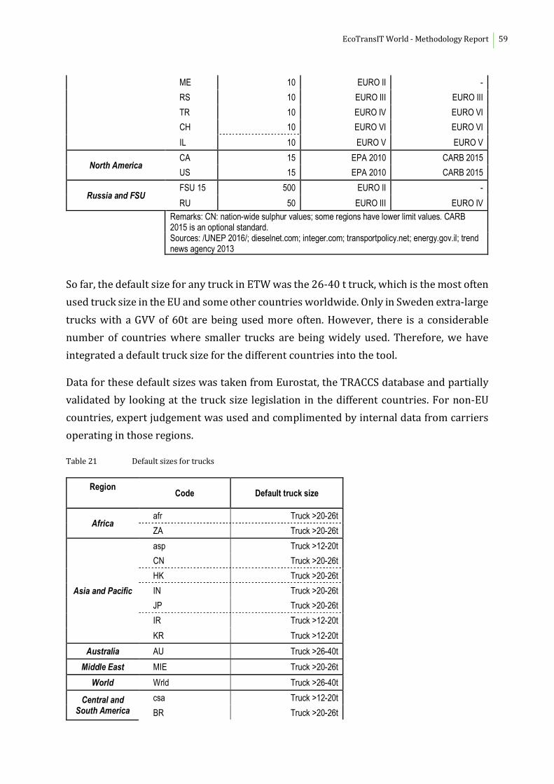
EcoTransIT World - Methodology Report 59
ME 10 EURO II -
RS 10 EURO III EURO III
TR 10 EURO IV EURO VI
CH 10 EURO VI EURO VI
IL 10 EURO V EURO V
North America CA 15 EPA 2010 CARB 2015
US 15 EPA 2010 CARB 2015
Russia and FSU FSU 15 500 EURO II -
RU 50 EURO III EURO IV
Remarks: CN: nation-wide sulphur values; some regions have lower limit values. CARB 2015 is an optional standard. Sources: /UNEP 2016/; dieselnet.com; integer.com; transportpolicy.net; energy.gov.il; trend news agency 2013
So far, the default size for any truck in ETW was the 26-40 t truck, which is the most often
used truck size in the EU and some other countries worldwide. Only in Sweden extra-large
trucks with a GVV of 60t are being used more often. However, there is a considerable
number of countries where smaller trucks are being widely used. Therefore, we have
integrated a default truck size for the different countries into the tool.
Data for these default sizes was taken from Eurostat, the TRACCS database and partially
validated by looking at the truck size legislation in the different countries. For non-EU
countries, expert judgement was used and complimented by internal data from carriers
operating in those regions.
Table 21 Default sizes for trucks
Region Code Default truck size
Africa afr Truck >20-26t
ZA Truck >20-26t
Asia and Pacific
asp Truck >12-20t
CN Truck >20-26t
HK Truck >20-26t
IN Truck >20-26t
JP Truck >20-26t
IR Truck >12-20t
KR Truck >12-20t
Australia AU Truck >26-40t
Middle East MIE Truck >20-26t
World Wrld Truck >26-40t
Central and South America
csa Truck >12-20t
BR Truck >20-26t

EcoTransIT World - Methodology Report 60
CL Truck >12-20t
MX Truck >20-26t
Europe
eur Truck >26-40t
BA Truck >26-40t
EU 28 (without SE) Truck >26-40t
ME Truck >26-40t
SE Truck >50-60t
RS Truck >26-40t
TR Truck >26-40t
CH Truck >26-40t
IL Truck >20-26t
North America CA Truck >60,000-80,000lbs
US Truck >60,000-80,000lbs
Russia and FSU rfs Truck >26-40t
RU Truck >26-40t
6.1.3 Final energy consumption and vehicle emissions (TTW)
For road transport with trucks, the general calculation rules described in chapter 4.3 are
applied. A speciality is the dependence of final energy consumption and vehicle emissions
from load weight:
The energy consumption and emissions of a truck depend on the specific energy
consumption of the vehicle per kilometre and increases with higher load weights. Thus,
the energy consumption per kilometre is a function of the capacity utilisation.
The following figure shows an example for the energy consumption per vehicle-km as a
function of load weight, including values for freight types.

EcoTransIT World - Methodology Report 61
Figure 13: Energy consumption for heavy duty trucks (40 t vehicle gross weight, Euro-V, motorway, hilly) as a function of load weight
Remark: Load for volume/average/bulk goods including empty trips Source: Handbook Emission Factors for Road Transport 4.1 (INFRAS 2019)
For the calculation of energy consumption and emissions per net tonne km, the basic
calculation rules are applied (see chapter 4.3).
Table 22 shows one set of TTW energy and emission values. For the calculation of TTW
CO2- and CO2e-emissions the default values of EN 16258 are applied (see Table 59 in the
appendix, chapter 7.1)
ECFempty
CU = 0%
ECF = ECFempty+ (ECFfull - ECFempty) * CU
ECFfullCU = 100%
ECFCU = M / CP
Definitions:ECF Final energy consumption with actual load (g/km)ECFempty Final energy consumption without load (g/km)ECFfull Final energy consumption with full load (g/km)
M Mass of freight (t)CP Payload capacity (t)CU Capacity utilisation (weight load / load capacity)

EcoTransIT World - Methodology Report 62
Table 22 Energy consumption and emissions (TTW) of selected diesel trucks with different load factors in Europe (Motorway, average gradient for hilly countries)
empty Average* full
Vehicle Type 0% 60% 100%
Energy Consumption (MJ/km)
Truck Euro VI >3,5-7,5t 6,1 6,7 7,1 >7,5-12t 6,5 7,3 7,8 >12-20t 7,2 8,7 9,7 >20-26t 7,8 9,8 11,2 >26-40t 8,5 11,9 14,4 >40-50t 9,3 13,9 17,2
>50-60t 11,5 16,8 20,4
>60t 15,0 23,3 29,3
NOx-Emissions (g/km)
Truck >26-40t Euro-I 7,7 10,5 12,3 Euro-II 7,9 10,7 12,6 Euro-III 5,9 8,1 9,7 Euro-IV 3,7 3,9 4,6 Euro-V 2,4 2,6 2,8 Euro-VI 0,6 0,4 0,5
NMHC-Emissions (g/km)
Truck >26-40t Euro-I 0,483 0,473 0,497 Euro-II 0,318 0,314 0,333 Euro-III 0,304 0,286 0,305 Euro-IV 0,026 0,032 0,036 Euro-V 0,036 0,040 0,044 Euro-VI 0,015 0,019 0,023
PM-Emissions (g/km)
Truck >26-40t Euro-I 0,269 0,329 0,377 Euro-II 0,129 0,163 0,192 Euro-III 0,148 0,149 0,172 Euro-IV 0,038 0,044 0,047 Euro-V 0,038 0,043 0,046 Euro-VI 0,010 0,009 0,009
Source: Handbook Emission Factors for Road Transport 4.1 (INFRAS 2019) *average usage not including empty trips
Rigid lorries and articulated trucks in the same gross weight class can have different
empty weights, depending on the body type (e.g. curtainsider vs. box). Thus, the user of
EcoTransIT World can enter their own empty weights into the calculation. Using an
interpolation, emission factors for slightly different truck masses were derived from the
original HEBFA 4.1 data.

EcoTransIT World - Methodology Report 63
6.1.4 Alternative fuel trucks
Worldwide the vast majority of the trucks uses diesel as fuel. Due to the potential emission
reductions and lower fuel costs some fleet managers invested into alternative fuels
recently. In 2014 around 200,000 heavy or medium-heavy trucks in Europe (most of them
in Eastern Europe) and 350,000 heavy or medium-heavy trucks in China were using CNG
or LNG according to the natural gas vehicle association (NGVA). Electric trucks are even
less common but have a growing importance (see Table 23).
Table 23 Market situation for trucks with alternative fuels
Drivetrain Market share worldwide
Examples for pioneer markets
Examples for truck manufacturers
Diesel Market leader worldwide all CNG Niche China, USA, Sweden e.g. IVECO, MAN, Daimler, SCANIA,
Renault, Volvo, Cummins Westport, Freightliner
LNG Niche China, USA, Netherlands, Spain
IVECO, SCANIA, Cummins Westport, Freightliner
Dual Fuel (CNG/LNG - Diesel)
Niche China, USA, UK MAN, Cummins Westport
Battery electric Niche Germany, Austria MAN, IVECO, Daimler (test)
Overhead catenary Pilot phase Sweden, Germany, USA Siemens (test), Scania Fuel cell Pilot phase Germany, USA Daimler, Volvo
Source: ifeu analysis
Having already a niche market, the truck types given in Table 24 are included in
EcoTransIT. LNG trucks are common for heavy trucks (>26 t GW) while battery trucks are
used for smaller size classes (<26 t). Being a rather young technology, only gas-powered
trucks with Euro V or Euro VI standard are considered. For dual fuel, truck manufacturers
so far have hesitated in bringing Euro VI dual fuel trucks on the market due to the
challenge of keeping the emission limits /DLR et al. 2015/.
Table 24 Truck types with alternative fuels in EcoTransIT
Drivetrain Size (gross vehicle weight) Emission standard
CNG 3,5-40 t EEV/Euro V Euro VI
LNG 26-40 t EEV/Euro V Euro VI
Dual Fuel (LNG/Diesel) 26-40 t EEV/Euro V Electric (Battery) 3,5-40 t -

EcoTransIT World - Methodology Report 64
Availability of refuelling infrastructure
CNG and LNG trucks require a dedicated refuelling infrastructure which is not yet
available in a similar amount to diesel stations or not available at all in some countries4.
Also, fast charging stations for battery vehicles, especially trucks, are not yet common.
Therefore, the operation of trucks with alternative fuels is limited to certain routes and
applications at the moment. EcoTransIT has no information on the spatial availability of
alternative fuel stations and ETW users have to check availability by themselves. It has to
be noted, that extra distances for refuelling might also increase the emissions.
Table 25 gives the number of CNG and LNG stations in the countries with the highest
density of these stations per 1000 km². The number of CNG stations is in most countries
higher than for LNG stations. However, the CNG stations are often designed for light duty
vehicles and the availability for trucks can be much lower.
When calculating a transport chain EcoTransIT provides the number of refuelling stations
in a starting country. But as mentioned above, the exact availability for a specific transport
chain (or route) has to be checked from other source, e.g. www.gibgas.de for the EU or
www.afdc.energy.gov for the USA.
4 However, the installation of a fuel infrastructure is supported by some countries, e.g. in
the EU for CNG and LNG within the next decade in order to fulfill the alternative fuel
infrastructure directive (2014/94/EU).

EcoTransIT World - Methodology Report 65
Table 25 Availability of CNG and LNG refuelling stations in the top 10 countries respectively (ranked by the number of stations per 1000 km²)
Fuel Region Country Stations Stations per 1000 km²
CNG
Europe Netherlands 194 5.72
Europe Switzerland 167 4.18
Europe Italy 1,022 3.47
Europe Germany 892 2.56
Europe Austria 205 2.49
Europe Luxembourg 6 2.32
Europe Czech Republic 173 2.24
Europe Belgium 56 1.85
Asia and Pacific South Korea 196 1.63
Asia and Pacific Iran 2,360 1.54
LNG
Europe Netherlands 16 0.47
Asia and Pacific China (including Hong Kong) 3,500 0.38
Europe United Kingdom 14 0.06
Europe Spain 25 0.05
Europe Portugal 4 0.04
Europe Italy 6 0.02
Europe Sweden 6 0.01
Europe France 7 0.01
Europe Germany 3 0.01
North America United States 76 0.01
Source: EU: NGVA, 2017 data; Non-EU: NGV Global, 2014 data
Specific energy consumption and emissions of alternative fuel trucks (TTW)
Only a few measurements are available already for alternative fuel trucks Due to the
current lack of information, instead of detailed energy consumption and emission factors
(i.e. per size class, road type and load), average correction factors compared to similar
diesel trucks are applied (see Table 26).
CNG and LNG trucks have higher specific energy consumptions than diesel, mainly due to
the lower energy efficiency of the stoichiometric spark ignition engine used for most gas
trucks. Based on a review of literature and fleet park operator’s data in /DLR et al. 2015/
a 24% higher energy consumption compared to diesel trucks is assumed. Dual fuel trucks
use compression ignition (diesel) engines and are therefore assumed to have the same
fuel efficiency than diesel trucks. The average ratio of natural gas (LNG) to diesel in energy
consumption of dual fuel trucks for ETW is 60:40, based on /DLR et al. 2015/ and own
assumptions.
Less information is available on real world air pollutant emissions (NOx, NMHC and PM)
of gas trucks. It is assumed that the emissions are similar to the diesel trucks, except that

EcoTransIT World - Methodology Report 66
Euro V CNG and LNG trucks have lower PM emissions, which are similar to Euro VI diesel
trucks. This is due to the fact that spark ignited gas engines have very low PM emissions,
even without using particle filters /TNO 2017/. The SOx emissions depend on the sulphur
content, which is assumed to be 3.5 ppm and therefore lower than for diesel /TNO 2011/.
Table 26 TTW emission factors of alternative fuel compared to diesel trucks
Vehicle Type (fuel, size, emission standard) EC NOx NMHC PM
CNG, all size classes, Euro V +24% similar Euro VI CNG, all size classes, Euro VI +24% similar LNG, all size classes, Euro V +24% similar Euro VI LNG, all size classes, Euro VI +24% similar
Dual Fuel (LNG/Diesel), all size classes, Euro V similar Source: (DLR et al. 2015), ifeu assumptions
Integration of gas-powered trucks into HBEFA 4.1 is still at an early stage, but follows a
similar methodology with simple correction factors comparing gas to diesel trucks. It was
thus decided to stick with the previously done assessment of the environmental
performance of gas trucks.
It has to be mentioned that the given assumptions provide only a rough picture and
include uncertainties which can be hardly quantified at the moment. With increasing
market entrance of alternative fuel trucks and availability of measurement data the
emission factors should be reviewed.
Furthermore, the processes for energy generation greatly differ for the different truck
types (see chapter 6.6 on WTT emissions). These emissions have to be included for an
adequate comparison of emissions, especially for electric trucks. Emissions from vehicle
construction are not yet within the scope of EcoTransIT, but can have a relevant share of
lifecycle emissions, i.e. for batteries (see also chapter 3.3.1).
Battery electric trucks are newly integrated into the HBEFA 4.1. They have no tailpipe
emissions and use electricity as their only fuel. The assessment for those trucks was done
using the VECTO model, their energy demand is however modelled for a potential future
vehicle (2025+) since battery-electric trucks are almost non-existent today. These
battery- electric trucks provide a range of 350 km and have a higher empty weight than
their conventional counterparts due to the addition of the battery.

EcoTransIT World - Methodology Report 67
Table 27 TTW energy consumption of electric trucks
Size Class Empty 0%
Average 60%
Full 100%
Truck <7.5t 2,7 3,0 3,2 Truck 7.5-12t 2,9 3,2 3,4
Truck 12-20t 3,3 3,6 3,8 Truck 26-40t 5,3 6,2 6,7
Source: Handbook Emission Factors for Road Transport 4.1 (INFRAS 2019)
6.2 Rail transport
The main indicator for calculating energy and emissions of rail transport is the energy
consumption of the total train depending on the gross tonne weight of the train and the
relation of net-tonne weight to gross tonne weight. In ETW this was taken into
consideration by using different general train types, defined by the gross tonne weight of
the train and different freight types (average, bulk, volume). In addition to this general
approach, the actual version of ETW allows to use special train types for dedicated
transport tasks.
6.2.1 Train Types
6.2.2 General train types
European railway companies have 1,000 t as a typical average gross weight for
international trains /UIC 2009/. The maximum gross weight for international traffic is up
to 2,000 tonnes.
In several countries outside Europe the typical gross tonne weight is significantly higher
e.g. Australia, Canada, China, USA. Typical train weights in these countries are about
4,000 tonnes and more. For this reason, ETW must cover a wide range in regards to train
weight.
Table 28 Definition of general train types in ETW
Train type Gross tonne weight train
Empty weight wagon
Capacity wagon
LF ETF
Light 500 t
23 t 61 t Bulk: 100 %
Average: 60% Volume: 30%
Bulk: 80 % Average:
50%Volume: 20%
Average 1000 t Large 1500 t Extra Large 2000 t
Heavy 5000 t

EcoTransIT World - Methodology Report 68
Source: ETW definitions and assumptions
6.2.3 Train types for dedicated transport tasks
For dedicated freight transports (cars, container, several solid bulks and liquids) special
trains and wagon types are used. Typical train configurations come from transport
statistics of major railway companies /DB Schenker 2012, SNCF 2012/. In ETW average
values for these train types are used. They mainly reflect the European situation.
Table 29 Definition of dedicated train types in ETW
Train type Gross tonne weight train
Empty weight wagon
Capacity wagon
LF ETF
Car 700 t 28 t 21 t 85 % 50 %
Chemistry 1200 t 24 t 55 t 100 % 100 %
Container 1000 t 21 t 65 t 48 % 20 %
Double Container 2500 t 25 t 100 t 48 % 20 %
Rolling Road - Truck 1200 t 25.4 t 70 t 42 % 20 %
Rolling Road - Semi Trailer 1200 t 34.3 t 100.7 t 47 % 20 %
Rolling Road - Swap Body 1200 t 34.3 t 100.7 t 39 % 20 %
Coal and steel 1700 t 26 t 65 t 100 % 100 %
Building materials 1200 t 22 t 54 t 100 % 100 %
Manufactured products 1200 t 23 t 54 t 75 % 60 %
Cereals 1300 t 20 t 63 t 100 % 60 %
Source: DB Cargo, SNCF, ifeu assumptions
6.2.4 Final energy consumption (TTW)
In ETW energy functions are used, which are verified by average values from different European railways. To take the different topologies of the European countries into account, three types of functions are used, which shall represent a “flat” (Denmark, Netherlands, Sweden), “mountain” (Austria, Switzerland) or “hilly” (all other countries) topology. For ETW, the function was updated with new values and a special survey for heavy trains (>2,000 tonnes).
The following energy consumption data for trains were available:
- Average annual consumption of typical freight transport by different companies, e.g.
data from UIC energy statistics (last update 2007) /UIC 2009/.
- Analysis of energy consumption of more than 200,000 rides of freight trains by Railion
in 2007 in different production types and train weight classes /Railion 2007/.
- Survey of train rides at the Gotthard line by SBB, mainly model calculations; values
between 17 and 23 Wh/Gtkm /SBB 2006/.

EcoTransIT World - Methodology Report 69
- Canada: statistics about annual average energy consumption of freight trains. In 2003
the average energy consumption of diesel freight trains was recorded as 33 Wh/Gtkm
and 61 Wh/Ntkm (average train weight in UIC-statistic 2007: about 5000 gross
tonnes) /EPS 2005/.
- China: average energy consumption of extra-large double deck container and normal
trains: Diesel 27 Wh/Gtkm, Electric 10 Wh/Gtkm (train weight about 4000 gross
tonnes) /ifeu 2008/.
- US Track1: statistics about annual energy consumption of freight trains; in 2006 the
average energy consumption of diesel freight trains was recorded as 66 kWh/Ntkm
(average train weight in UIC-statistic 2007: about 5000 gross tonnes) /USDOT 2008/.
- The EX-TREMIS study, which is a kind of “official” dataset for Europe, proposed a
function for rail freight transport, which is similar to EcoTransIT methodology
/TRT 2008/.
The following diagram shows some of the values mentioned above, compared to the
former function of EcoTransIT (hilly). The following conclusions can be stated:
- Nearly all values reside below the former EcoTransIT function.
- The function of EX-TREMIS stays very close to the Railion values in a range from 600
to 1800 gross tonnes.
- Some values from UIC statistics are higher than the Railion values, but the majority
are in line with it.

EcoTransIT World - Methodology Report 70
Figure 14: Energy consumption of electric trains – data sources
Energy consumption of electric trains – data sources (Wh/Gtkm)
Source: Railion, UIC, ifeu
ETW function includes the following assumptions:
- For train weights between 600 and 1800 gross tonnes, the Railion values correlate
well with the function of EX-TREMIS and most of the UIC-values. Therefore, the
following function correlated to these values was calculated:
ECspec [Wh/Gtkm] = 1200 * GTW-0,62
(ECspec: specific Energy Consumption, GTW: Gross Tonne Weight)
- Below 600 gross tonnes, the diffusion of the values is higher. This means a higher
uncertainty of the values. We propose to use the same function as for the middle
weight trains in order to define the function as simply as possible.
- Above 1500 gross tonnes, the Railion values show no significant reduction of specific
energy consumption with growing train weight. This general trend is confirmed by
values of heavy trains (4000 gross tonnes and more) for Canada, China and USA.
Therefore, we propose to use the function until 2200 gross tonnes (specific energy
value: 10 Wh/Gtkm) and keeping it constant for larger trains.
0
5
10
15
20
25
30
35
40
45
50
55
60
65
200 400 600 800 1000 1200 1400 1600 1800 2000 2200 2400
Hilly 2003
Railion 2007
EX-TREMIS 2008
UIC Railway Data 2007

EcoTransIT World - Methodology Report 71
- The function is valid for “hilly” countries. For flat countries, the values of the function
are multiplied by 0.9, for mountainous countries the factor is 1.1.
The following figure shows the resulting new functions compared to the EcoTransIT “Hilly
2003” function.
Figure 15 Functions for the energy consumption of electric trains
Energy consumption of electric trains – Functions in ETW (Wh/Gtkm)
Source: EPS, Railion, TRT, UIC, USDOT, ifeu
The specific energy consumption per net tonne km is calculated for each train type with
the following formula:
Specific energy consumption [Wh/Ntkm] =
Energy consumption of train [Wh/Gtkm] /
Relation Nt/Gt of freight (including empty trip factor)
Relation Nt/Gt = 0.40 for volume freight
0.52 for average freight
0.60 for bulk freight
The following figure shows the specific energy consumption as a function of the net
tonnes/gross tonne relation for a 1000-tonne electric train and the values for each freight
type.
0
5
10
15
20
25
30
35
40
45
50
200 400 600 800 1000 1200 1400 1600 1800 2000 2200 2400
Hilly 2003Hilly 2009
Flat 2009Mountain 2009

EcoTransIT World - Methodology Report 72
Figure 16 Specific energy consumption of an electric train of 1,000 Gt as function of load factor and values for each freight type
Specific energy consumption of an electric train of 1,000 Gt as function of load factor and values for each freight type
Remark: Load for volume/average/bulk goods including empty trips
Source: EPS, DB Cargo, TRT, UIC, USDOT, ifeu
The following table shows the specific energy consumption of the default electric trains
for each freight type.
0
10
20
30
40
50
60
70
80
90
100
0 2 4 6 8 10 12 14 16 18 20 22 24 26 28 30 32 34 36 38 40 42 44 46 48 50 52 54 56 58 60
Load weight (t)
Sp
ecif
ic e
nerg
y co
nsu
mp
tio
n (
Wh
/tkm
)
volume
averagebulk

EcoTransIT World - Methodology Report 73
Table 30 Specific final energy consumption for selected electric trains
Final Energy Consumption
Train Type Train Freight Bulk Average Volume
Unit Wh/Gtkm Wh/Ntkm General trains
Light Train (500t) 25.5 42.7 49.5 63.9 Average Train (1000t) 16.6 27.8 32.2 41.5 Large (1500t) 12.9 21.6 25.0 32.3 Extra Large (2000t) 10.8 18.1 20.9 27.0 Heavy (>2000t) 10.0 16.8 19.4 25.1 Dedicated trains Car 20.7 69.3 Chemistry 14.8 27.7
Container 16.6 30.0 Double Container 10.2 16.3 Rolling Road - Truck 14.8 30.0 Rolling Road - Semi Trailer 14.8 27.7
Rolling Road - Swap Body 14.8 30,3 Coal and steel 11.9 21.5 Building materials 14.8 26.8 Manufactured products 14.8 28.2
Cereals 14.1 21.2 Including vessel weight (container, truck, semi-trailer, swap body) Source: DB Cargo, SNCF, ifeu assumptions
6.2.5 Energy consumption of diesel trains
The available energy data for diesel traction ranges between 2.6 and 9.7 g/gross tonne
km /Railways companies 2002/. New statistics show a similar range /UIC 2009/. The
statistical uncertainties can be attributed to the unreliable allocation of the fuel
consumption to different users (passenger and goods transport, shunting, etc.).
Therefore, the primary energy consumption of diesel traction is estimated on the basis of
the primary energy consumption of electric traction. This procedure can be used, because
the total efficiency of diesel traction (including the production of fuel) is similar to the
total efficiency of electric traction (including electricity generation).
So, the same functional dependence as that of electric traction is taken and has to be
divided by the efficiency of the diesel-electric conversion for final energy consumption of
37 %. (See Chapter 6.6.1).
The following table shows the resulting specific energy consumption per Gtkm and Ntkm
for different diesel trains and freight types. Some available values of heavy trains from
China and statistical averages for Canada and USA are added. The values of North

EcoTransIT World - Methodology Report 74
American railways are higher than values from energy function (similar to the large train
in the formula). For this reason, additional energy consumption for North American
railways could be possible, but we propose to use this formula also for North America as
well on account of the small North American database available.
Table 31 Specific final energy consumption for diesel trains
Final Energy Consumption
Train Type Train Freight Bulk Average Volume
Unit Wh/Gtkm Wh/Ntkm Light Train (500t) 68.8 115.5 133.7 172.6 Average Train (1000t) 44.8 75.2 87.0 112.3 Large (1500t) 34.8 58.4 67.6 87.3 Extra Large (2000t) 29.1 48.9 56.6 73.1 Heavy (>2000t) 27.0 45.4 52.5 67.8
Values of heavy trains Average (not specified)
China 2008 27 Canada 2003 33 61
US Track 1 2006 66 Source: DB Cargo, ifeu EPS 2005, USDOT
Emission factors for diesel train operation (TTW)
Similar to diesel engines for road and inland ship transport, the emission performance of
locomotive engines strongly depends on the engine technology. In the past years the UIC,
the EU and US implemented emission limits for new engines in several stages, thus
reducing specific emissions for newer engines. This fact should be considered in ETW by
providing different emission factors by emissions stage, like already available for road
and inland ship transport.
The following table lists the relevant emission stages and emission factors of the UIC, the
European Union and the US-EPA.

EcoTransIT World - Methodology Report 75
Table 32: Emission standards for diesel trains (NOx, NMHC, PM)
Standard Manufacture year HC NOx PM
International UIC (g/kWh)
UIC 1 <=2002 0,8 12
UIC 2 2003-2008 0,8 9,5 0,25
European Union, P>560 kW (g/kWh)
Stage IIIa 2009-2011 0,5 6,0 0,2
Stage IIIb/V >=2012 0,2 3,8 0,025
US-EPA, line-haul (g/bhp.hr)
Non regulated <1973 0,5 13,5 0,34
Tier 0 1973-1992 1,0 8,0 0,22
Tier 1 1993c-2004 0,6 7,4 0,22
Tier 2 2005-2011 0,3 5,5 0,10
Tier 3 2012-2014 0,3 5,5 0,10
Tier 4 >2015 0,1 1,3 0,03
Source: www.dieselnet.com
Determination of emission factors for ETW
For ETW these values can be transformed to fuel-related emission factors. Typical energy
consumption values for locomotive engines are about 210 g/kWh [IFEU, 2003], therefore
this value is used for the transformation.
For ETW a PM value for UIC 1 is added, based on engine data from engines with
manufacture year 1997 and before from [IFEU, 2003]. Table 33 shows the resulting
emission factors used in ETW.

EcoTransIT World - Methodology Report 76
Table 33: Emission factors for diesel locomotives (freight transport) in ETW available in the expert mode
Standard Manufacture year HC NOx PM
International: UIC (g/kg)
UIC 1 <=2002 3,8 57,1 1,56
UIC 2 2003-2008 3,8 45,2 1,19
European Union, >560 kW (g/kg
Stage IIIa 2009-2011 2,4 28,6 0,95
Stage IIIb/V >=2012 1,0 18,1 0,12
US-EPA, line-haul (g/kg)
Non-regulated <1973 4,1 73,8 1,53
Tier 0 1973-1992 7,8 44,0 0,97
Tier 1 1993c-2004 4,5 41,0 0,97
Tier 2 2005-2011 2,2 30,2 0,48
Tier 3 2012-2014 2,2 18,6 0,37
Tier 4 >2015 0,5 4,8 0,11
Source: www.dieselnet.com; own assumptions
Country specific regulations and default values
The emissions values in Table 33 can be compared with existing data from railway
companies and the recent default values of EcoTransIT (see Table 34). The comparison
shows, that the former ETW-values have a level between UIC 1 and UIC 2 and the average
cargo fleet of DB in 2015 lies between UIC 2 and Stage IIIa. Other data could not be
evaluated so far.
Table 34: Emission factors for diesel locomotives (freight transport) from different sources
Standard Manufacture year HC NOx PM
Average values (g/kg), different sources
ETW 2010 All 4,6 48,3 1,30
DB 2016 All 2,6 42 0,96
Due to the lack of a sophisticated survey, we propose a simple approach for default values
in ETW:
- For USA and Canada, the Tier 2 standard is used as default value
- For Germany the DB 2016 value is used
- For other EU 27 countries the emission factors of the UIC 2 standard are applied
- For all other countries the UIC 1 standard is assumed.
For future improvement we recommend to ask the UIC for country specific emission
factors, which can be used as default values.

EcoTransIT World - Methodology Report 77
Option: particle filter
Several locomotives are equipped with a particle filter, which reduces PM-emissions
considerably. For this reason, the extended mode in ETW gives an additional option to
choose a particle filter. As default a value of 0.012 g PM/kg is used.
6.2.6 Shunting
In ETW shunting processes to collect and distribute freight wagons are not included in
the calculation. Furthermore, the same is true for feeder trains, because private tracks
from factory to the switch yard are not part of the routing in ETW.
Some railway companies have statistics about the operation performance and energy
consumption for shunting. However, the effort can be very different for each transport
process. Hence average values for a company are not suitable for a specific transport task.
The collection and distribution of wagons for single wagon trains is done on marshalling
yards. A shunting locomotive, mainly with diesel traction, collects several groups of
wagons and pushes them to a marshalling hump. Moved by the gradient, the wagons roll
down to the tracks of the dedicated train, navigated by the control center which chooses
the track.
The energy consumption for shunting is calculated for a typical shunting cycle (MTU-
shunting), which is described in [ifeu 2003].
The following assumptions are made for a shunting process:
- Shunting locomotive, diesel, power 1000 kW
- Moving 15 wagons to the marshalling hump
- Total time of shunting process: 15 minutes (including empty runs of locomotive)
- Average motor load: 16% (MTU shunting standard)
- Average fuel consumption: 280 g/kWh (BR 290, [ifeu 2003])
- Resulting total fuel consumption: 11.2 kg diesel / 15 wagons
= 0.75 kg diesel / wagon = 32 MJ diesel / wagon
The total fuel consumption per wagon has to be allocated to the dedicated freight in one
or several wagons.

EcoTransIT World - Methodology Report 78
6.3 Sea transport
6.3.1 Overview
The sea transport emission factors in ETW are largely based on the findings of the Third
Greenhouse Gas study of the International Maritime Organization (IMO) /IMO 2015/.
Basically, fuel consumption and emission factors for main engine, auxiliary engine and
boiler were derived in a bottom-up approach from IMO data for individual ship categories
and size classes and validated using worldwide fuel consumption and CO2 emissions for
2012 from /IMO 2015/. These factors were then aggregated to
a) the vessel types and size classes available in the Extended input mode of ETW (Table 41), and
b) the world trade lanes, which are automatically assigned based on the chosen origin and destination, for the Standard mode of ETW.
The resulting fuel consumption and emission factors are further adjusted to a default or
user-specified speed reduction and cargo utilization.
The following vessel types are differentiated:
- General Cargo Vessels
- Dry Bulk Carriers
- Liquid Bulk Carriers
- Container Carriers
- Roll-on-Roll-off vessels
Other vessels are not included in ETW because of their differing cargo specifications and
lower relevance for the likely ETW user. Those vessel types include LNG and LPG gas
carriers as well as car carriers. Ferries are not included in this section of the report
because they are treated like extensions of the road network and are thus presented in
the chapter on land transport.
6.3.2 Derivation of basic fuel consumption and emission factors
The basic fuel consumption and emission factors are derived for each IMO ship type and
size class, separately for main engine, auxiliary engine, and boiler, based on the
methodology used in the Third IMO Greenhouse Gas Study from 2015 (see /IMO 2015, p.
43ff/ for ship types and associated parameters).

EcoTransIT World - Methodology Report 79
In order to account for emissions in port and return journeys, fuel consumption is
modelled separately for main engine, auxiliary engine, and boiler, for a virtual one-year
period in the standard assumption. The results are normalized to one tonne-kilometre
(i.e. expressed in g/tkm). If reduced vessel speeds are modelled, the vessel’s activity
extends the one-year period in order to deliver the same transport services (see Chapter
6.3.4).
The fuel consumption in g/tkm of the main engine is derived based on the following
formula:
���� = �(�ℎ × ��� × ( � × ���� ��⁄ ) (��� × ��))⁄
With ���� = Fuel consumption of the main engine in g/tkm
�ℎ = Share of vessel stock per engine age group � [%] based on age distribution5.
The engine age groups are listed in Table 35.
��� = Specific fuel consumption in g/kWh per engine age group � /IMO 2015/.
The respective values are displayed in Table 35.
� = Average nominal power for the ship type and size class [kW] /IMO 2015/.
���� = Load factor at design speed with clean hull and in calm weather (90% MCR
for all ships based on /IMO 2009/)
�� = Design speed /IMO 2015/.
��� = Average payload capacity in dead weight tonnes /IMO 2015/
�� = Cargo utilization [%] based on /IMO 2009/
For ships classes with up to 15 MW average installed power, the specific fuel consumption
values for MSD (medium-speed diesel) engines in Table 35 are applied, and for larger
ships the values for SSD (slow-speed diesel) engines /Williams et al. 2008/.
5 Separate age distributions for ships up to 50’000 dwt and above 50’000 dwt were
derived from a sample of 4616 vessels from the Lloyds Register of Ships /Lloyds 2009/.

EcoTransIT World - Methodology Report 80
Table 35: Main engine fuel consumption factors (values in g/kWh; IMO 2015, p. 109).
Engine age group Engine rating
SSD MSD HSD
Before 1983 205 215 225 1984–2000 185 195 205 post-2001 175 185 195
The fuel consumption in g/tkm of auxiliary engine and boiler is calculated as follows:
��,� =�((���� × 24 × ����) + #�$%&' × 24 × �$%&')( × ) × ���,�*
+,-
With ��,� = Fuel consumption of the auxiliary engine or boiler in g/tkm
���� = Number of days at sea per year /IMO 2015/
���� = Auxiliary engine/boiler load at sea [kW] /IMO 2015/
�$%&' = Number of days in port per year
�$%&' = Auxiliary engine/boiler load in port [kW], /IMO 2015/
) = Number of auxiliary engines /IMO 2015/ (for boilers: ) = 1)
���,� = Specific fuel consumption of the auxiliary engine or boiler in g/kWh
(Table 35).
tkm = Avg. annual transport performance per ship in tonne-kilometres
Table 36: Auxiliary engine/boiler fuel consumption factors (values in g/kWh; IMO 2015, p. 109).
Engine type
Fuel type
HFO MDO
Auxiliary engine 225 225 Steam boiler 305 300
Emission factors in g/g fuel for the different pollutants considered in ETW, differentiated
by main engine and auxiliary engine/boiler as well as fuel type (HFO or MDO) and engine
rating, are based on /IMO 2015/ and can directly be multiplied with the fuel consumption
factors derived above. They are listed in Table 37 for the main engine and Table 38 for
auxiliary engines and boilers.

EcoTransIT World - Methodology Report 81
For NOx, SOx and PM, the emission factors depend on the sulphur content of the fuel used.
For HFO, the sulphur content is assumed to be 2.51% /IMO 2015/, and for MDO, 0.1%
(limit valid from 1st of January 2015; see also Chapter 6.3.5).
Table 37: Main engine emission factors (values in g/g fuel; IMO 2015).
Pollutant IMO Tier Engine rating
Fuel type Emission
factor [g/g fuel]
NOx 0 SSD HFO 0.09282 1 SSD 0.08718 2 SSD 0.07846 0 MSD 0.06512 1 MSD 0.06047 2 MSD 0.05209
SOx All SSD 0.04908 All MSD 0.04910
PM All SSD 0.00699 All MSD 0.00639
NMHC All SSD 0.00308 All MSD 0.00233
CO2 All SSD 3.11000 All MSD 3.11000
CO2eq All SSD 3.15000 All MSD 3.15000
NOx 0 SSD MDO 0.05817 1 SSD 0.05463 2 SSD 0.04917 0 MSD 0.04081 1 MSD 0.03789 2 MSD 0.03264
SOx All SSD 0.00176 All MSD 0.00176
PM All SSD 0.00068 All MSD 0.00062
NMHC All SSD 0.00308 All MSD 0.00233
CO2 All SSD 3.21000 All MSD 3.21000
CO2eq All SSD 3.24000 All MSD 3.24000

EcoTransIT World - Methodology Report 82
Table 38: Auxiliary engine/boiler emission factors (values in g/g fuel; IMO 2015).
Pollutant IMO Tier Engine rating
Fuel type Emission
factor [g/g fuel] NOx 0 MSD HFO 0.06476
1 MSD 0.05727 2 MSD 0.04934
SOx All MSD 0.04908 PM All MSD 0.00603 NMHC All MSD 0.00176 CO2 All SSD 3.21000
All MSD 3.21000 CO2eq All SSD 3.24000
All MSD 3.24000 NOx 0 MSD MDO 0.04058
1 MSD 0.03589 2 MSD 0.03092
SOx All MSD 0.00176 PM All MSD 0.00059 NMHC All MSD 0.00176 CO2 All SSD 3.21000
All MSD 3.21000 CO2eq All SSD 3.24000
All MSD 3.24000
6.3.3 Aggregation to ETW size classes and trade lanes
Depending on the input mode (Standard or Extended), different aggregation levels or fuel
consumption and emission factors are required in ETW.
In the Standard mode, the user only specifies origin and destination of the cargo, as well
as the cargo type (bulk or containers). Based on this, the appropriate trade lane/cargo
type combination (see Table 39) is automatically chosen. Consequently, average fuel
consumption and emission factors representative for the chosen trade lane have to be
applied.
In the Extended input mode, the user can choose ship type and size, as well as the goods
type and the handling (see Table 41). Hence, the fuel consumption and emission factors
for the ship types and size classes available in the Extended input mode of ETW have to
be available.
a) Trade lanes
For the aggregation to trade lanes, the fuel consumption and emission factors are
calculated as a tkm-weighted average of the ships operating on the respective trade lane
based on their size. The required input activity data (mileage, capacity, cargo utilization)

EcoTransIT World - Methodology Report 83
are based on /IMO 2009, 2015/. Table 39 lists all region pairs considered by ETW and
defines the trade lanes. The associated aggregated size classes are listed in
Table 40. The Standard mode does not differentiate liquid and dry bulk.

EcoTransIT World - Methodology Report 84
Table 39: Overview of region pairs and respective trade lanes considered by ETW.
From / To EU -
Europe NA -
North Am. LA -
Latin Am. AF -
Africa AS - Asia
OZ - Oceania
EU - Europe
Intra-con-tinental Europe
Transatlantic trade
Other global trade
Other global trade
Suez trade
Other global trade
NA - North Am.
Transatlantic trade
Intra-con-tinental (non
Europe)
Panama trade
Other global trade
Transpacific trade
Other global trade
LA - Latin Am.
Other global trade
Panama trade
Intracontinental (non Europe)
Other global trade
Other global trade
Other global trade
AF - Africa
Other global trade
Other global trade
Other global trade
Intracontinental (non Europe)
Other global trade
Other global trade
AS - Asia
Suez trade
Transpacific trade
Other global trade
Other global trade
Intracontinental (non Europe)
Other global trade
OZ - Oceania
Other global trade
Other global trade
Other global trade
Other global trade
Other global trade
Intracontinental (non Europe)
Table 40: Default vessel categories depending on cargo type and trade lane
Vessel types
Trade lane
Aggregated size class
BC (liquid, dry, and General Cargo) Suez trade Aframax / Suezmax BC (liquid, dry, and General Cargo) Transatlantic trade Handymax / Panamax BC (liquid, dry, and General Cargo) Transpacific trade Handymax / Panamax / Aframax / Suezmax BC (liquid, dry, and General Cargo) Panama trade Handymax / Panamax BC (liquid, dry, and General Cargo) Other global trade Handysize / Handymax / Panamax / Aframax BC (liquid, dry, and General Cargo) Intra-continental trade Feeder / Handysize / Handymax CC Suez trade 4,700 – 7,000 (+) TEU CC Transatlantic trade 2,000 – 4,700 TEU CC Transpacific trade 1,000 – 7,000 (+) TEU CC Panama trade 2,000 – 4,700 TEU CC Other global trade 1,000 – 3,500 TEU CC Intra-continental trade non EU 500 – 2,000 TEU CC Intra-continental trade EU 500 – 2,000 TEU Great Lake BC < 30,000 DWT
Note: BC = bulk carrier, GC = general cargo ship, CC = container vessel
The ship size ranges per trade lane are based on a sample analysis of transport services
of ocean carriers6. Size differentiation can be particularly found in container trade,
6 The following carrier schedules were analysed to develop the vessel size
groupings per major trade lane: a) Container carriers: NYK Line, OOCL, Hyundai

EcoTransIT World - Methodology Report 85
whereas bulk transport depends more on the type of cargo and distance sailed. The major
container trades are distinctive in terms of volumes and goods; therefore, different vessel
sizes are deployed on those trades. For example, the Europe – Asia container trade is
dominated by large container ships above 5,000 TEU. North America is linked with Asia
with a broader range of vessels, usually above 3,000 TEU. In both trade lines ultra-large
container vessels are used (above 14,500 TEU), too. In the Europe – North America trades
the bulk numbers of container vessels are between 2,000 and 4,700 TEU. Europe trades
with the African and Latin American continent are dominated by vessels between 1,500
and 4,000 TEU capacity. For other trade lanes, an average “international” emission factor
was formed and several intra-continental emission factors were developed (see
Table 40).
A similar approach was used for bulk vessels. However, the distinction here is based on
certain size restrictions in particular regions. Some installations in the world sea
infrastructure restrict the size of the vessels. The most important ones were considered
in developing the vessel size classes for bulk vessels. These are the Suez Canal, the Panama
Canal, and the entrance to the Baltic Sea. The Suez Canal does not pose a restriction to
even the largest container ships. However, bulk carriers are limited to approximately
200,000 DWT. The Panama Canal poses both restrictions for bulk carriers (ca. 80,000
DWT) and container ships (ca. 4,300 TEU with some vessels up to 5,000 TEU capacity).
However, it is currently under construction – after its expansion, it is expected to
accommodate container ships of up to 13,000 TEU. The Baltic Sea entrance is limited to
bulk vessels of maximum 120,000 DWT in general. However, the ports in the Baltic Sea
are mostly served by smaller feeder vessels7. Furthermore, the Baltic Sea as well as the
North Sea are so-called Emission Control Areas (ECAs) with limits on fuel sulphur at sea
and in port /Sustainable Shipping 2009/ (see Chapter 6.3.5 for the consideration of ECAs).
b) Size classes in the extended input mode of ETW
The vessel types and size classes available in the Extended input mode of ETW are listed
in Table 41. The ETW vessel types are identical to the ship types in /IMO 2015/, but the
Merchant Marine, APL, CMA-CGM, Hapag Lloyd; b) Bulk carriers: Sea bulk, Polar, AHL
Shipping Company. Additionally, ship tracking websites like www.marinetraffic.com
were consulted.
7 Personal communication Port of Oslo.

EcoTransIT World - Methodology Report 86
size class boundaries differ in some cases. For this aggregation, an equal distribution of
dead-weight tonnage within the IMO size classes is assumed. The aggregation is carried
out (as for the trade lines) by tkm-weighted averaging of all emission factors by the ETW
size classes. with the input activity data (mileage, capacity, cargo utilization) based on
/IMO 2009, 2015/.
Table 41: Vessel types and sizes that can be selected in the Extended input mode of ETW.
Vessel types (and cargo handling)
Trade and Vessel category names
Aggregated size class
GC Coastal < 5,000 DWT BC / GC (dry) Feeder 5,000 – 15,000 DWT BC / GC (dry) Handysize 15,000 – 35,000 DWT BC (dry) Handymax 35,000 – 60,000 DWT BC (dry) Panamax 60,000 – 80,000 DWT BC (dry) Aframax 80,000 – 120,000 DWT BC (dry) Suezmax 120,000 – 200,000 DWT BC (liquid) Feeder 5,000 – 15,000 DWT BC (liquid) Handysize 15,000 – 35,000 DWT BC (liquid) Handymax 35,000 – 60,000 DWT BC (liquid) Panamax 60,000 – 80,000 DWT BC (liquid) Aframax 80,000 – 120,000 DWT BC (liquid) Suezmax 120,000 – 200,000 DWT BC (liquid) VLCC (+) > 200,000 DWT CC Feeder <1,000 TEU CC like Handysize 1,000 – 2,000 TEU CC EU SECA like Handysize 1,000 – 2,000 TEU CC like Handymax 2,000 – 3,500 TEU CC like Panamax 3,500 – 4,700 TEU CC like Aframax 4,700 – 7,000 TEU CC like Suezmax 7,000 – 14,500 TEU CC ULCV >14,500 TEU Global average CC World over all ships RoRo RoRo small < 5000 DWT RoRo RoRo large >= 5000 DWT (BC = bulk carrier; CC = container vessel; GC = general cargo ship; RoRo = Roll-on/roll-off ship; VLCC = very large crude carrier; ULCV = ultra-large container vessel)
6.3.4 Adjustments for speed and cargo utilization
Ship speed is one of the most sensitive parameters in the calculation of fuel consumption
and emissions of sea transport. Due to the over-proportional reduction in fuel
consumption compared to the service speed, “slow steaming” has become a widespread
practice in sea transport – in 2012, the average ratio of operating speed to design speed
75% /IMO 2015/. Cargo utilization, on the other hand, is sensitive since ETW calculates

EcoTransIT World - Methodology Report 87
shipment-specific emissions, and obviously these are reduced the more goods the
emissions can be divided by.
In the Standard mode, the operating speed and the cargo utilization are determined by
trade lane and corresponds to the tkm-weighted averages per IMO ship type and size class
/IMO 2009, 2015/. In the Extended input mode, the user can adjust speed and cargo
utilization of sea transport. The speed adjustment is expressed in percent reduction
relative to the chosen ship’s design speed. The cargo utilization is expressed in percent of
capacity.
Regardless of whether inputs are default or user-specified, the fuel consumption and
emission factors in ETW are adjusted based on the equations described in the following
paragraphs.
a) Adjustment for speed
The main engine load is adjusted based on the speed reduction relative to design speed
(based on /IMO 2009, 2015/):
���1' = (2�1' 2���)⁄ 3 × 0.9 × 1.09 × 1.15
With ���1' = Load factor given actual speed [%]
2�1' = Actual speed [km/h]
2��� = Design speed [km/h]
The constant 0.9 corresponds to the engine load at design speed (with clean hull and calm
weather). The factor 1.09 accounts for hull roughness and the factor 1.15 for wave
resistance in average conditions /IMO 2015/.
Once the engine load under the actual speed is known, the fuel consumption and emission
factors are adjusted. The adjustment is carried out according to the following formula. It
adds up the fuel consumption (or emissions, respectively) of main engine, auxiliary engine
and boiler, and accounts for the parabolic dependency of specific fuel consumption on
engine load /IMO 2015, Jalkanen et al. 2012/ as well as for the additional time at sea due
to slower speed:
��9: = (�� × ���1' 0.9⁄ ) × #0.455 × ���1'; − 0.71 × ���1' + 1.28( × (1 (1 − 2�1' 2���⁄ )⁄ ) + #�.��� + ��,���( × (1 (1 − 2�1' 2���⁄ )⁄ ) + (�,?%&'+ ��,?%&')

EcoTransIT World - Methodology Report 88
With ��9: = Speed-adjusted fuel consumption or emission factor [g/tkm]
�� = Fuel consumption or emission factor of the main engine [g/tkm]
�.��� = Fuel consumption or emission factor of the auxiliary engine at sea
[g/tkm]
��.���= Fuel consumption or emission factor of the boiler at sea [g/tkm]
�.?%&'= Fuel consumption or emission factor of the auxiliary engine in port
[g/tkm]
��,?%&'= Fuel consumption or emission factor of the boiler in port [g/tkm]
b) Adjustment for cargo utilization
The speed-adjusted fuel consumption and emission factors are adjusted for the deviation
of cargo utilization from the default using:
�@AB�C = ��9: × (����@ ���1'⁄ )
With �@AB�C = Cargo utilization-adjusted final fuel consumption or emission factor
[g/tkm]
����@ = Default cargo utilization (/IMO 2009/, tkm-weighted average for the
respective trade lane or ETW ship type and size; see Table 42) [%]
���1' = Actual cargo utilization [%]

EcoTransIT World - Methodology Report 89
Table 42: Default parameters used in ETW per trade lane (Standard mode) or vessel type/size class (Extended mode).
Vessel type (and cargo handling)
Trade (Standard mode) / Size class (Extended mode)
Days at sea
Design speed [km/h]
Default speed [km/h]
Default cargo
utilization [%]
BC (liquid/dry/general) Suez trade 200 29.0 22.3 55%
BC (liquid/dry/general) Transatlantic trade 182 28.2 22.2 54%
BC (liquid/dry/general) Transpacific trade 194 28.7 22.1 54%
BC (liquid/dry/general) Panama trade 182 28.2 22.2 54%
BC (liquid/dry/general) Other global trade 186 28.3 22.0 52%
BC (liquid/dry/general) Intra-continental trade 172 27.3 21.3 53%
CC Suez trade 248 47.9 30.2 70%
CC Transatlantic trade 236 44.6 29.8 70%
CC Transpacific trade 245 47.0 30.1 70%
CC Panama trade 236 44.6 29.8 70%
CC Other global trade 236 44.6 29.8 70%
CC Intra-continental trade non EU 210 39.4 27.3 70%
CC Intra-continental trade EU 190 30.6 23.0 70%
Great Lakes BC - 238 26.3 19.7 58%
GC Coastal 161 21.5 16.1 60%
BC (dry) Feeder 167 25.9 19.6 56%
BC (dry) Handysize 171 28.4 21.7 55%
BC (dry) Handymax 173 28.6 21.9 52%
BC (dry) Panamax 188 28.5 22.1 52%
BC (dry) Aframax 191 28.5 22.0 53%
BC (dry) Suezmax 199 28.4 21.7 56%
BC (liquid) Feeder 173 25.5 20.6 62%
BC (liquid) Handysize 175 26.8 21.8 59%
BC (liquid) Handymax 184 28.0 22.8 62%
BC (liquid) Panamax 214 30.6 24.8 64%
BC (liquid) Aframax 204 29.8 23.5 58%
BC (liquid) Suezmax 211 30.2 23.3 57%
BC (liquid) VLCC (+) 232 29.8 23.5 50%
CC Feeder 190 30.6 23.0 70%
CC like Handysize 200 36.1 25.7 70%
CC like Handymax 219 42.5 28.6 70%
CC like Panamax 236 44.6 29.8 70%
CC like Aframax 244 46.1 30.1 70%
CC like Suezmax 250 48.9 30.2 70%
CC ULCV 251 46.3 27.4 70%
CC World 236 45.1 29.4 70%
RoRo RoRo small 146 19.8 16.3 70%
RoRo RoRo large 209 34.4 26.3 70%
Global average CC World 210 33.3 24.7 58%
6.3.5 Consideration of emission control areas (ECAs)
Emissions from sea vessels are regulated in Annex VI of the “International Convention on
the Prevention of Pollution from Ships”, also known as MARPOL. Annex VI defines two

EcoTransIT World - Methodology Report 90
sets of emission and fuel quality requirements: on one hand global requirements, and on
the other hand more stringent requirements applicable in so-called Emission Control
Areas (ECAs). An ECA can be designated for SOx, PM, or NOx, or all three pollutants, subject
to a proposal from a Party to Annex VI.
Existing Emission Control Areas include /Dieselnet 2015/:
- Baltic Sea (SOx, adopted: 1997; entered into force: 2005)
- North Sea (SOx, 2005/2006)
- North American ECA, including most of US and Canadian coast (NOx & SOx,
2010/2012).
- US Caribbean ECA, including Puerto Rico and the US Virgin Islands (NOx & SOx,
2011/2014).
The fuel sulphur limits inside and outside ECAs are depicted in Figure 16. ECA-specific NOx emission limits enter into force from 2016 but are not yet considered in ETW.
Different options exist to comply with the emission limits in ECAs. Currently the most
widespread is to use Marine Diesel Oil (MDO), which has a sulphur content of 0.1%
(compare Chapter 6.3.2). Other options are to use scrubber, an after-treatment
technology that uses sea water to wash SO2 out of the exhaust gas, or to switch to LNG
instead of diesel. However, the latter two options are not very widespread: as of January
2015, only 0.6% of the world fleet was fitted with scrubbers /Fathom 2015/, and even
fewer ships used LNG.
In ETW, it is therefore currently assumed that all ships comply with ECA emission limits
(as well as special emission limits in ports) by switching to MDO. This is implemented by
splitting the journey travelled into the distance within and outside ECAs. For the distance
within ECAs, the fuel consumption and emission factors for MDO (Marine Diesel Oil) are
applied, and for the distance outside, the factors for HFO (Heavy Fuel Oil; see Table 36 –
Table 38).
Besides ECAs, stricter emission limits also apply to certain ports, e.g. all ports in Europe
and California. Ports in other parts of the world have voluntary fuel switch programs,
which offer incentives like reduced port fees for using lower-sulphur fuels. The maximum
allowed sulphur level in these programs varies. As a simplified assumption, MDO (with
0.1% sulphur content) is assumed to be used in ports with stricter emission limits or
voluntary fuel switch programs, i.e.:
- All ports in Europe

EcoTransIT World - Methodology Report 91
- All ports in California
- Seattle, New York, New Jersey, Houston (USA)
- Vancouver (Canada)
- Hong Kong
- Singapore
Figure 17 MARPOL Annex VI fuel sulphur limits (source: Dieselnet 2015).
6.3.6 Allocation rules for seaborne transport
The emissions of ocean-going vessels are averaged over the entire return journeys, taking
the load factors and empty returns into account. All emissions are allocated to the freight
carried.
For bulk vessels the allocation unit is tonne-kilometre (tkm). All emissions are allocated
to the product of transported tonnes of freight and distance travelled. The emissions of
container vessels are calculated on a container-kilometre basis (TEU-km). tkm and TEU-
km are converted to each other using the container weights presented in Table 9 for
volume, average and bulk goods.
6.3.7 Ferry transport
Ferry transport is a special case within ETW as it represents a “hybrid” mode of transport,
i.e. it is road or rail transport on a ship. ETW handles ferry routes as an extension of the
road and rail network. The user of the web interface cannot choose “ferry” as a mode, but
ferry transport is chosen automatically when the mode is road or rail and the most

EcoTransIT World - Methodology Report 92
advantageous route leads via a ferry route (compare Chapter 5.2). In the extended mode,
the user can choose whether to explicitly avoid or prefer ferry routes. The description of
ferry transport is placed in the sea transport chapter in this report since the basic
methodology and source of the pollutant emission factors is the same as for sea transport
(see Chapter 6.3.2).
The allocation of the energy consumption between passenger and goods transport is a
tricky and controversial issue. Different allocation methodologies have been proposed
(e.g. /Kristensen 2000/ or /Kusche 2000/); the decision which is the most appropriate
cannot be made objectively but remains a convention. In conformity with the European
norm (EN) 16258, ETW allocates the energy consumption to freight according to the
share of deck area dedicated to vehicles.
The final fuel consumption per gross tonne-kilometre of cargo (i.e. allocated to each tonne
of cargo inside the ferry including the vehicle, i.e. train or truck, in g/tkm) is calculated
based on the following equation:
��1�&D%, D&%�� = ##��E�&&F × �E&�ADG'( (�� × ��)⁄ (
All input parameters for this equation have been derived based on two studies from the
Baltic and Mediterranean Seas, i.e. /Scandria 2012/ and /Holmegaard and Hagemeister
2011/. Their values are displayed in Table 43.
Table 43: Parameters for the calculation of final fuel consumption of cargo on ferries.
Parameter Description Unit Value
��1�&D% Final fuel consumption per gross tonne kilometre g/tkm 14.1
��E�&&F Total fuel consumption of the ferry (main and auxiliary engines) g/km 86,971
�E&�ADG' Share of freight in terms of deck area dedicated to vehicles % 54%
�� Cargo capacity of the ferry [t] t 5,218
�� Cargo capacity utilization of the ferry % 64%
The fuel consumption per net tonne-kilometre (i.e. allocated only to the weight of goods
transported inside the train or truck) is calculated by dividing the fuel consumption per
gross tonne-kilometre by the ratio of the weight of the goods transported to the weight of
the vehicle including the goods transported (compare Chapters 6.1 and 6.2):
��1�&D%, B�' = ��1�&D%, D&%�� #-1�&D% -(H�GA1C�I1�&D%)⁄ (⁄
where:
��1�&D%, B�' = final fuel consumption per net tonne kilometre [g/tkm]

EcoTransIT World - Methodology Report 93
��1�&D%, D&%�� = final fuel consumption per net tonne kilometre [g/tkm]
-1�&D% = mass of cargo on the vehicle (truck, train) [t]
-(H�GA1C�I1�&D%) = mass of the vehicle (truck, train) including cargo [t]
The same pollutant emission factors in g/g fuel have based on /IMO 2015/ are used as for
other sea transport (see Chapter 6.3.2), assuming a share of 65% of the main engine in
total fuel consumption (based on /IMO 2015/).
6.4 Inland waterway transport
6.4.1 Overview
The methodology for inland waterway transport has been updated compared to previous
versions of ETW (see /ifeu, INFRAS, IVE 2014/). The main focus was to consider up to
date fuel consumption and emission factors data and update ETW where necessary.
Inland vessels are modelled in a bottom-up approach similar to ocean-going vessels (see
Chapter 6.3). However, instead of applying tkm-weighted average fuel consumption and
emission factors for aggregate ETW classes, four representative ship types are provided:
- The Europa ship, representative for ships with up to 1500 t capacity, and used by
default on rivers of CEMT Classes I-IV8;
- The “Grossmotorschiff”, representative for ships with 1500 – 3000 t capacity, and used
by default on rivers of Class V;
- The Jowi class, representative for capacities >3000 t, used by default on rivers of Class
VI.
- A 2x2 push convoy (Push boat and 2x2 “Europa” barges) with a capacity of 11’200 t,
representative for convoys and selectable on rivers of class V and above.
8 Large navigable waterways are classified by the CEMT standard created by the
European Conference of Ministers of Transport (Conférence Européenne des Ministres
des Transports) in 1992 /CEMT 1992/. The standard specifies the maximum measures
(length, bean, draught, tonnage) for ships to be able to navigate on rivers of each class.
EcoTransIT World - Methodology Report 94
This approach is more appropriate given the lack of activity data on inland navigation
(especially outside Europe), which would have added uncertainty to any tkm-weighted
aggregation. For Europe, a comparison of mean fuel consumption factors with tkm-
weighted aggregated classes has shown that the three ship types listed above represent
their size classes well. World-wide, a comparison of EcoTransIT emission factors with a
report commissioned by the Global Logistics Emission Council (GLEC, STC-Nestra 2018)
has shown deviations ranging from -28% to about +38%, to the average CO2 emission
factors by ship type cited from several studies for China, the U.S. and the Rhine basin. It
should be noted that the assumptions on speed, cargo capacity utilization, or
inclusion/exclusion of auxiliary engine fuel consumption in the sources cited by STC-
Nestra (2018) are partially unknown, which may explain some of the differences.
The resulting fuel consumption and emission factors are further adjusted to a default or
user-specified cargo utilization.
6.4.2 Inland waterways in ETW
The majority of waterways available in ETW are located in Europe. All European
waterways class IV and above are included in ETW (Figure 18). Most prominent are the
rivers Danube, Elbe, Rhine, and Seine9, which are (at least in sections) classified as CEMT
class VI. Other rivers and canals in Europe are classified as class V or smaller. The
distinction between inland waterways up to class IV and above is important because the
size and carrying capacity of inland barges significantly increases on class V and larger
rivers.
9 There are other smaller sections that are technically “inland waterways” but are
treated as part of the ocean network in ETW. Those include the Weser up to Bremerhaven
or the North-Baltic-Channel.

EcoTransIT World - Methodology Report 95
Figure 18: European inland waterways and their classification
Worldwide, approximately 50 countries have navigable waterways of more than 1000 km
length. Inland freight navigation is underdeveloped in many countries /BVB 2009/.
Besides Europe, mainly the USA and China exhibit significant inland waterway transport
performance /Amos et al. 2009/. ETW enables inland waterways calculation on the
largest global waterways, such as the Yangtze, Mississippi or Amazon rivers. The CEMT
classification is not available on non-European waterways; therefore, the class V is
assigned per default to all waterways outside Europe (Figure 19).
Figure 19: Worldwide inland waterways in ETW.

EcoTransIT World - Methodology Report 96
6.4.3 Derivation of basic fuel consumption and emission factors
As for sea transport, fuel consumption is modelled separately for main and auxiliary
engine for a virtual one-year period in order to account for emissions in port and return
journeys and normalized to one tonne- or TEU-kilometre.
The fuel consumption of the main engine is calculated as follows:
��� = ((� × ��JK) 2⁄ ) (�� × �LM)⁄ × ���
With ��� = Fuel consumption of the main engine [g/tkm or g/TEU-km]
� = Installed power [kW] /Panteia 2013/
��JK = Load factor at default cargo utilization /ifeu and INFRAS 2013/
2 = Speed [km/h] /ifeu and INFRAS 2013/
�� = Default cargo utilization /ifeu and INFRAS 2013/
�LM = Capacity (dead weight tonnage or TEU) /Panteia 2013/
��� = Specific diesel consumption in g/kWh (200 g/kWh for all ships based on
/ifeu and INFRAS 2013/)
The input data related to the inland vessel fleet (nominal power, capacity) are sourced
from /Panteia 2013/ and correspond to averages of the EU fleet. Load factors, cargo
utilization is based on the German TREMOD model /ifeu and INFRAS 2013/. The load
factor at default cargo utilization is calculated from ship type- and size class-specific load
factors at full or empty load and for up- and downstream travel, respectively, that were
derived for TREMOD from empirical data on energy consumption from German river
sections /ifeu and INFRAS 2013, BMVBS 2011/:
��JK = ���N$'F + #���N$'F − ��@OCC( × ��
With ��JK = Load factor at default cargo utilization
���N$'F = Average load factor at empty load
��@OCC = Average load factor at full load

EcoTransIT World - Methodology Report 97
The average load factors at empty/full load are calculated as the arithmetic average of the
respective up- and downstream load factors.
The fuel consumption of the auxiliary engine is assumed to be 5% of the consumption of
the main engine, as in TREMOD /ifeu and INFRAS 2013/.
Technical data on the three inland barge types provided in ETW are listed in Table 44.
Table 44 Inland vessel technical parameters
Vessel type Default for
CEMT river class
Length [m]
Beam [m]
Installed power [kW]
Average speed [km/h]
Capacity Default cargo utilization
DWT (bulk)
TEU (Con-tainer)
Bulk Con- tainer
Europa ship I - IV 85 9.5 737 10.5 1'350 100 60% 60% Great Engine Vessel V 110 11.4 1'178 10.5 2'500 200 50% 60% JOWI class VI+ 135 17.34 2'097 10.5 5'300 450 50% 60%
2x2 push convoy selectable on VIb+
195 22.8 3’264 10.5 11’200 820 50% 60%
The emission factors for inland vessels have been updated compared to /ifeu, INFRAS, IVE
2014/). Similar to diesel engines for road and rail transport, the emission performance of
inland vessel engines strongly depends on the engine technology. In the past years the EU
and US implemented emission limits for new engines in several stages, thus reducing
specific emissions for newer engines. This fact should be considered in ETW by providing
different emission factors by emissions stage, like already available for road transport.
Table 45 lists the emission stages and emission factors available for ETW. The factors have
been derived from measurements and literature data for European ships in /ifeu and
INFRAS 2013/. For the more recent stages US Tier 3 and US Tier 4, values have been
derived from the emission limits and certification data by the EPA in 2014 and 2015 for
category 1 and 2 engines /EPA 2015/.
Table 45 Inland vessel engine emission factors
Emission stage (manufacture year) NOx (g/kWh) NMHC (g/kWh) PM (g/kWh)
conventional (1970-2002) / US Tier 1 11,67 0,52 0,32
CCNR I (2002-2006) 9,00 0,39 0,12
CCNR II/ EU IIIA / US Tier 2 (>2006) 7,00 0,29 0,12
US Tier 3 5,10 0,28 0,12
US Tier 4 1,4 0,06 0,03
Source: /ifeu and INFRAS 2013/, /EPA 2015/, dieselnet.com, ifeu assumptions

EcoTransIT World - Methodology Report 98
According to evaluations in /ifeu and INFRAS 2013/ it was estimated that the average
engine age for German and Dutch ships in 2011 was around 20 years. It can further be
estimated that currently more than half of the transport performance in Germany is
carried out by ships with no type approved engines (thus older than 2002). Also, most
countries outside Europe or the US have no regulation for inland ship engines. Thus, the
stage “conventional (1970-2002) / US Tier 1” is used as default value. For Germany, which
may be representative for Western Europe, this will result in slightly higher emissions
than for the average fleet. However, expert users can calculate emissions with newer
emission stages if they have detailed knowledge of the ship or engine age.
6.4.4 Allocation rules for inland waterway transport
For inland waterway navigation, the same allocation rules as for ocean transport apply
(see Chapter 6.3.6).
6.5 Air transport
6.5.1 Type of airplanes and load factor
The type and model of airplanes (e.g. Boeing 747-400, B777F) used for air cargo has a
high impact on GHG emissions and air pollutants. On the one hand the type gives the
information about the capacity of the airplane and age of the turbine used. On the other
hand, the aircraft type delivers information if air cargo is transported in dedicated
freighters (only for freight) or together with passengers in aircrafts (so-called belly
freight). This information is important for the allocation methodology (see subchapter
6.5.4). In the extended input mode of ETW 42 dedicated freighter and some 200
passenger aircraft types are available for selection. For the full list of aircraft type refer
to the table the appendix 7.4.
Each aircraft is characterised by both a maximum possible design range and a maximum
payload (maximum freight weight). Large passenger aircrafts can fly without stopovers
more than 10,000 km, whereas smaller ones have maximum ranges of 2,000 to 3,000
km /Lang 2009/. Aside from that, larger aircrafts can transport more freight than
smaller ones. The maximum payload capacity of larger aircrafts is much higher. ETW
includes a wide range of small, medium and large aircrafts covering the whole possible
spectrum of operating distances and payloads, which is shown exemplarily for selected
freighter aircraft in Fehler! Verweisquelle konnte nicht gefunden werden.. ETW

EcoTransIT World - Methodology Report 99
considers only the so-called design range of the aircrafts, which is the maximum range
for the case if the whole structural payload is utilised /Hünecke 2008/. Beyond this
range the payload has to be reduced due to the additional fuel needed for the longer
flight. This possibility is not considered by ETW.
Figure 20 Design ranges and maximum payload capacities of selected dedicated air freighters
Within the extended input mode ETW provides only aircrafts suitable for the flight
distance between the selected airport pair. If the trip distance is longer only those
aircrafts are offered by ETW that are able to fly this distance. The longer the flight, the
fewer the types of aircrafts provided (see Fehler! Verweisquelle konnte nicht
gefunden werden.). Additionally, the aircraft are distinguished between dedicated
freighter and passenger aircrafts. The characteristics of all freighter and passenger
aircrafts included in EcoTransIT are available in Table 62 in the annex. In the extended
input mode of ETW, all aircraft types are available and may be chosen by the user.
In the standard input mode of ETW, an own selection of airplanes is not possible. Rather,
ETW use the airplanes of Table 46 depending on the flight distance (up to 1,000 km short
haul aircraft; over 1,000 km up to 3,700 km medium haul aircraft; more than 3,700 km
long haul aircraft). Because to the users of the standard input mode it is usually
unknown whether a dedicated freighter or passenger aircraft is used, ETW uses a mix of
both aircraft types. This mixed aircraft type is called “hybrid aircraft”. Worldwide
between 40% and 48% of freight ton-kilometres in air cargo is transported by freighter
/lower value Statista 2018; higher value ICAO 2018/. The lower value is used for the
hybrid aircrafts of EcoTransIT independent of flight distance. Thus, if a user of the
standard input mode selects airports EcoTransIT calculates firstly the distance of the
Airbus A300-600F
Airbus A310F
Airbus A330-200F
ATR 72-200FBAe 146F
Boeing (douglas) MD-11F
Boeing 727F
Boeing 737-300F
Boeing 747-200F Boeing 747-400F
Boeing 747-8F
Boeing 757-200PF
Boeing 767-200F
Boeing 777-200F
0
20
40
60
80
100
120
140
160
- 1,000 2,000 3,000 4,000 5,000 6,000 7,000 8,000 9,000
Des ign range i n km
Max. payl oad in tonnes
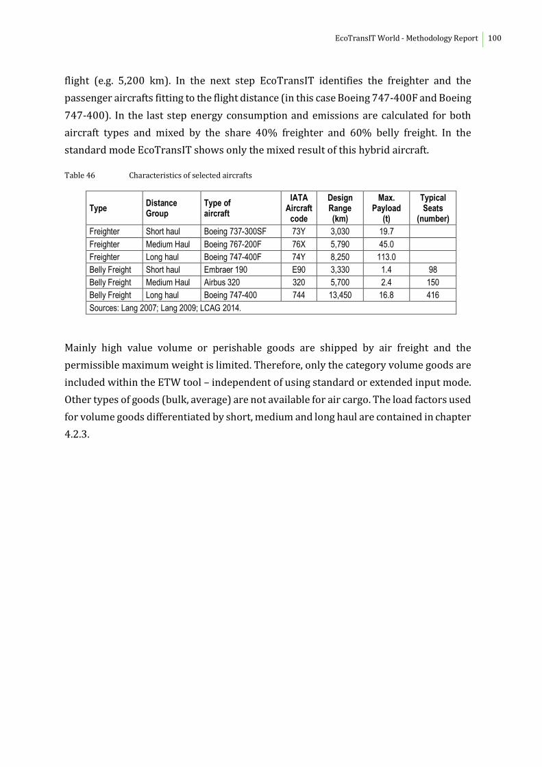
EcoTransIT World - Methodology Report 100
flight (e.g. 5,200 km). In the next step EcoTransIT identifies the freighter and the
passenger aircrafts fitting to the flight distance (in this case Boeing 747-400F and Boeing
747-400). In the last step energy consumption and emissions are calculated for both
aircraft types and mixed by the share 40% freighter and 60% belly freight. In the
standard mode EcoTransIT shows only the mixed result of this hybrid aircraft.
Table 46 Characteristics of selected aircrafts
Type Distance Group
Type of aircraft
IATA Aircraft
code
Design Range (km)
Max. Payload
(t)
Typical Seats
(number)
Freighter Short haul Boeing 737-300SF 73Y 3,030 19.7
Freighter Medium Haul Boeing 767-200F 76X 5,790 45.0 Freighter Long haul Boeing 747-400F 74Y 8,250 113.0 Belly Freight Short haul Embraer 190 E90 3,330 1.4 98 Belly Freight Medium Haul Airbus 320 320 5,700 2.4 150 Belly Freight Long haul Boeing 747-400 744 13,450 16.8 416
Sources: Lang 2007; Lang 2009; LCAG 2014.
Mainly high value volume or perishable goods are shipped by air freight and the
permissible maximum weight is limited. Therefore, only the category volume goods are
included within the ETW tool – independent of using standard or extended input mode.
Other types of goods (bulk, average) are not available for air cargo. The load factors used
for volume goods differentiated by short, medium and long haul are contained in chapter
4.2.3.

EcoTransIT World - Methodology Report 101
6.5.2 Energy consumption and emission factors (Tank-to-Wheel)
Specific TTW energy consumption and TTW emissions of air cargo transportation
depend heavily on the length of the flight. This is caused by different energy needs and
emissions in different phases of flight (e.g. take-off or climb). Due to the data sources
used by ETW this dependency from flight distance is considered for air pollutants like
NOx, NMHC and PM. For fuel consumption the data source used (EUROCONTROL “Small
Emitters Tool”, see below) only considers a linear correlation between energy
consumption and flight distance. This simplification is legitimate since most air cargo
flights are long haul flights where take-off and landing phases don’t dominate the overall
energy consumption of the whole flight. Furthermore, energy consumption and
emissions depend on utilisation of the capacity of aircrafts (utilisation of payload
capacity). Whereas this dependency is considered by road transport, this was not able
for aircrafts due to lack of available data. But the possible error is small and therefore
justifiable.
The basis of fuel consumption for the different airplanes considered by ETW is the
EUROCONTROL “Small Emitters Tool”10 which has been developed on behalf of the
European Commission for reporting under the European Emissions Trading Scheme
(ETS) /EUROCONTROL 2009,2015, 2017 and 2019/. This data source is updated yearly
and covers a wide range of aircrafts and aircraft families including many newer ones
/BEIS 2016/. The Small Emitters Tool covers more than 400 different aircraft types
including turboprop engines. EUROCONTROL gathers, on a regular basis and from
volunteer aircraft operators in Europe, samples of actual fuel-burn data for their flights
performed in a specific year (e.g. 2017). Based on this fuel-burn data a linear regression
is carried out for each aircraft type in the sample to consider the fuel dependency from
distance flown (see for example in Figure 21) /EUROCONTROL 2009/. In total measured
energy consumptions are available for around 85 different aircraft types in the Small
Emitters Tool.
In a second step the Small Emitters Tool uses conclusions by analogy for aircraft families.
That means that for aircrafts without measured fuel-burn data the energy consumption
of other aircraft types of the same family is used (e.g. fuel-burn data from B747-400 for
B747-300). In these cases, the measured data are adjusted by using a correction factor
based on the MTOW (maximum take-off weight) ratio /EUROCONTROL 2009/. This
10 See also http://www.eurocontrol.int/small-emitters-tool.

EcoTransIT World - Methodology Report 102
approach is used for around 30 airplanes. In a third step data from the EMEP/EEA Air
Pollutant Emission Inventory Guidebook (formerly called the EMEP CORINAIR Emission
Inventory Guidebook) is used for around 30 airplanes /EEA 2013, 2015 and 2019/. Last
but not least for the remaining aircraft types (around 270) the average fuel consumption
per flight kilometre is calculated based on linear regression model based on the available
data considering the MTOW of each airplane /EUROCONTROL 2009/.
Figure 21 TTW energy consumption of the Small Emitters Tool is based on a linear regression of fuel-burn data collected in Europe – example of a Boeing 747-400 /EUROCONTROL 2009/
Since the Small Emitters Tool contains only fuel-burn data for one aircraft model (e.g.
Boeing 747-400), the data is used for both dedicated freighter and passenger aircrafts
(see Table 47: Boeing 747-400F). Most of the energy consumption data of the 32
freighter and passenger aircrafts considered in ETW are based on measured fuel-burn
data collected in context of the Small Emitters Tool. Only for three aircrafts conclusions
by analogy from other family models are used (Boeing 777-200/200ER, Boeing 777F
and Boeing (McDonnell Douglas) MD-90). For four further aircraft types the method of
linear regression based on all available data is applied (Boeing 727F, Boeing 747-8F,
Boeing 747-8i and Boeing 787-8). Table 47 shows exemplarily the TTW energy
consumptions for the six airplanes used for calculation of the “hybrid aircrafts” in the

EcoTransIT World - Methodology Report 103
standard input mode of ETW relating to discrete travel distances. These energy
consumption values are completely based on measured fuel-burn data from the Small
Emitter Tool. For distances between the discrete mission distances given in Table 47
(e.g. between 4,630 and 5,556 km) the fuel consumptions of the aircrafts are calculated
by linear interpolation.
Table 47 TTW fuel consumption of selected freighter and passenger aircrafts depending on flight distances
Distance (km)
Dedicated freighter Passenger aircrafts
Boeing 737-300SF
(kg)
Boeing 767-200F
(kg)
Boeing 747-400F
(kg)
Embraer 190 (kg)
Airbus 320 (kg)
Boeing 747-400
(kg)
232 1,570 2,119 5,744 1,366 1,527 5,744
463 2,285 3,383 8,381 1,912 2,217 8,381
926 3,714 5,911 13,655 3,004 3,597 13,655
1,389 5,143 8,439 18,928 4,096 4,977 18,928
1,852 6,572 10,967 24,202 5,188 6,357 24,202
2,778 9,431 16,023 34,749 7,371 9,118 34,749
3,704 12,289 21,079 45,296 9,555 11,878 45,296
4,630 26,135 55,843 14,638 55,843
5,556 31,191 66,389 17,399 66,389
6,482 36,248 76,936 20,159 76,936
7,408 87,483 87,483
8,334 98,030 98,030
9,260 108,577
10,186 119,124
11,112 129,671
12,038 140,218
12,964 150,765
13,890 161,312
Source: EUROCONTROL Small Emitters Tool /EUROCONTROL 2017/
CO2, CO2 equivalents and SOx depend directly on the amount of kerosene consumed by the
airplanes. For CO2-equivalent the emission factors of the European standard EN 16258
are used without changes (see Table 48 and Table 59). The CO2 emission factor used by
ETW is based on the same sources than the CO2 equivalent emission factor included in the
European standard so that the CO2 emissions calculation of ETW is comparable with the
approach of EN 16258. For SOx an emission factor of 0.84 g per kg kerosene is applied for
ETW /EEA 2013/2015/. This value is based on data from EUROCONTROL. On national
level the values can be much lower. For example, in Germany an emission factor of 0.4 g
SO2 per kg kerosene in 1998 and 0.2 g SO2 per kg kerosene in 2009 is used /Öko-Institut
2010; ifeu and Öko-Institut 2012/.

EcoTransIT World - Methodology Report 104
Table 48: Fuel-based emission factors for CO2, CO2e and SOx (TTW) for kerosene (jet A and jet A1)
g/kg fuel
Carbon dioxide (CO2) 3.15 Carbon dioxide equivalents (CO2e) 3.18 Sulphur dioxide emissions (SOx) 0.84
Sources: EEA 2013/2015; EN DIN 2012; Öko-Institut 2010.
NOx, NMHC and PM are air pollutants which are independent from the fuel consumption
of the aircrafts. For these air pollutants ETW uses emission factors of the EMEP/EEA Air
Pollutant Emission Inventory Guidebook /EEA 2013/2015/. This guidebook provides
detailed emission factors for NOx, HC and PM of around 75 different aircraft types with
regard to discrete mission distances. The data of the EMEP/EEA Guidebook is applied in
different national inventories (e.g. see /ifeu and Öko-Institut 2012/ for Germany/ as
well as for several emission calculation tools (e.g. see /ICAO 2012/). In this context, it
has to be taken into account that the EMEP/EEA data is based on an average fleet. The
calculated values may be 10% below or above the real emissions of individual aircrafts
calculated for a concrete city pair /ICAO 2012/. Nevertheless, EMEP/EEA data is the
most comprehensive publicly available data source for NOx, HC and PM emissions of
aircrafts.
For ETW the emission data of the EMEP/EEA Guidebook are used directly without
changes /EEA 2013/2015/. Table 49 shows the results for the aircraft type Boeing 747-
400 according to the flight distance. Since the emission values are also given only for
discrete mission distances, emissions for flight distances between those listed in the
Table 49 are calculated by linear interpolation. In some cases, the data from the
EMEP/EEA Guidebook doesn’t cover the maximum ranges of the airplanes. For these
cases the emission values were extrapolated to cover the whole ranges needed for the
ETW calculations. These extrapolation steps were done by using a polynomial
regression. Because the EMEP/EEA Guidebook only includes distance related emission
factors for hydrocarbons in total (HC), NMHC emissions have to be calculated
afterwards. Therefore, it was assumed that the NMHC emissions for the Landing and
Take-Off cycle (so-called LTO cycle, <1,000 m altitude) be 90% of total HC emissions,
while during cruise only NMHC is emitted /EEA 2013/2015/. The NMHC values in Table
49 consider already this adjustment step.

EcoTransIT World - Methodology Report 105
Table 49 NOx, HMHC and PM emissions of aircraft type Boeing 747-400 (freighter)
Distance (km)
NOX (kg)
NMHC (kg)
PM (kg)
232 126 2.8 0.6
463 171 3.1 0.9
926 227 3.7 1.5
1,389 290 4.2 2.1
1,852 353 4.6 2.6
2,778 472 5.8 4.2
3,704 607 6.5 5.0
4,630 734 7.4 6.2
5,556 863 8.3 7.4
6,482 988 9.1 8.6
7,408 1.126 10.3 9.8
8,334 1.248 11.2 11.0
9,260 1.373 12.1 12.1
1,186 1.506 13.0 13.3
1,112 1.783 15.0 15.9
12,038 2.239 17.9 19.9
12,964 2.509 19.9 22.5
13,890 2.930 22.8 26.4
Sources: EEA 2013/2015; INFRAS calculations.
6.5.3 Emission Weighting Factor (EWF)
Some air pollutants (in particular nitrogen oxides, ozone, water, soot, sulphur) emitted
by aircrafts in cruising altitude can have an additional climate impact to CO2 /IPCC
1999/. To express these additional climate impact very often the so called “Radiative
Forcing Index” (RFI) is used. For cruise in critical altitudes over 9 kilometres the RFI
factor lies between 2 and 4 (on average 3). That means that the total climate impact of
the emissions of airplanes is twice or four times higher compared to the TTW CO2
emissions /UBA 2008; IPCC 2006/.
Disadvantage of the RFI is, that this factor considers only the present radiative forcing
of air pollutants and water vapour. This factor is inapplicable to calculate CO2 equivalent
emissions, because this indicator takes into account the global warming potential (GWP)
of emissions measured over a time period of 100 years. For this reason, the so-called
Emission Weighting Factor (EWF) was developed especially for air traffic. Similar to the
GWP, the EWF considers all additional climate effects of aircraft emissions compared to
CO2 over a time period of 100 years /Graßl and Brockhagen 2007/.

EcoTransIT World - Methodology Report 106
EWF is also applied for cruising in an altitude over 9 kilometres and lies between 1.2 and
2.7. For ETW the user can choose to consider the EWF for the calculation of the CO2
equivalent emissions. In this case an average EWF of 2.4 for flights over 9 kilometres is
used based on ifeu/Öko-Institut /2012/11. These altitudes are usually reached in the
cruise phase of flights with distances greater than approx. 400–500 km /Atmosfair
2007/. Therefore, in ETW the use of the EWF is only included as an option for flights
with distances over 500 km. The average EWF for the entire flight including take-off and
landing is listed in Table 50 according to the total flight distance.
In this context it has to be pointed out that considering EWF (or RFI) for the calculation
of CO2 equivalent emissions of air traffic is not compliant with the European standard
EN 16258. That means that results are only fully in accordance with EN 16258 without
considering EWF for calculation of CO2 equivalent emissions. This is the reason EWF
gives the user the possibility to additionally select EWF on their own responsibility. In
this case the user cannot state that the results are in line with EN 16258. For this reason,
the factor can only be calculated via the interfaces of the Business Solutions.
Table 50 Average Emission Weighting Factor (EWF) depending on flight distance
Distance (km)
Share of fuel used over 9 km
(%)
Average EWF
500 0% 1.00
750 41% 1.57 1,000 59% 1.83 2,000 76% 2.06 4,000 87% 2.21
10,000 94% 2.31 Sources: Graßl/Brockhagen 2007; Atmosfair 2009; ifeu/Öko-Institut 2012; INFRAS calculations.
6.5.4 Allocation method for belly freight
The energy consumption and emissions of dedicated freighters are simply allocated per
leg (airport pair) by using the quotient of air cargo weight considered and the total
payload within the aircraft. The latter is the product of maximum payload capacity (CP)
and the capacity utilisation (CU). For belly freight the energy consumption has to be split
11 In this case the TTW CO2 equivalent emissions are calculated by multiplication of
the TTW CO2 emissions with the factor 2.4

EcoTransIT World - Methodology Report 107
between air cargo and passenger. For the allocation of emissions between passenger and
freight different approaches are principally possible /EN 16258; ICAO 2012/. ETW uses
the approach used (and required) by the European Standard EN 16258. In accordance
with EN 16258 a weight of 100 kg (= 0.1 t) per passenger is assumed. Figure 22 contains
the concrete formula to allocate the energy consumption and emissions of passenger
aircrafts.
Figure 22 Allocation rules for dedicated freighter and passenger aircrafts in accordance with EN 16258
The approach required by EN 16258, which is used for belly freight, leads to higher fuel
consumption and emissions of air cargo carried by passenger aircrafts compared to that
of freighters. As Figure 23 shows, for aircrafts used for the standard input mode of ETW,
the CO2 emissions of belly cargo is 20 to 80% higher as air cargo transported by
dedicated freighters. Additionally, the figure shows that the specific CO2 emissions of
smaller aircrafts (e.g. B737-300SF) are much higher than those of larger aircrafts which
are used for long-haul flights (e.g. B 747-400F). In this context it has to be noted, that
small aircrafts are only used for short-haul trips up to 1.000 km, medium sized aircrafts
for medium-haul trips between 1.000 and 3.700 km, while big aircrafts are only used for
long-haul flights over 3.700 km within ETW.
Dedicated freighter
Passenger aircraft
Air cargo
Air cargo
mcargo
(CP x CUcargo + nseats x 0,1 t x CUpassanger)
mcargo
(CP x CUcargo)
mcargo = weight of air cargo considered [tons]
Passenger
Legend:
CP = maximum payload of cargo [tons]
CUcargo = capacity utilisation [%]
npassenger = number of seats offered [number]
CUpassenger = capacity utilisation passenger [%]

EcoTransIT World - Methodology Report 108
Figure 23 Specific TTW CO2 emissions of selected freighter and passenger aircrafts in g/tkm used for the ETW standard input mode /EUROCONTROL 2017; INFRAS calculations/
6.6 Energy consumption and emissions of the upstream
process (WTT)
Additional to the emissions caused directly by operating the vehicles (Tank-to-
Wheels/TTW) emissions and energy consumption of the generation of final energy
(fuels, electricity) are taken into account by ETW (Well-to-Tank/WTT). The impacts of
building the infrastructure for extraction and generation of the different energy carrier
are also included. Considering Tank-to-Wheels energy consumption and GHG emissions
as well as Well-to-Wheels energy consumption and GHG emissions (sum of TTW and
WTT) is a requirement of the European standard EN 16258. ETW provides TTW as well
as WTW data not only for energy consumption and GHG emissions, but also for all air
pollutants. Therefore, ETW provides emission data always in the same system boundaries
required by EN 16258.
The main energy carriers used in freight transport processes are liquid fossil fuels such
as diesel fuel, kerosene, heavy fuel oil and electricity. To compare the environmental
impacts of transport processes with different energy carriers, the total energy chain has
to be considered:
Energy chain of electricity production:
-
500
1,000
1,500
2,000
2,500
0 2,000 4,000 6,000 8,000 10,000
Embraer 190
Airbus A320
Boeing 747-400
(Passenger)
Boeing 737-300
(Freighter)
Boeing 767-200
Freighter
Boeing 747-400F
(Freighter)
g CO2e/tkm (TTW)
Fl ight distance in km

EcoTransIT World - Methodology Report 109
- Exploration and extraction of the primary energy carrier (coal, oil, gas, nuclear etc.)
and transport to the entrance of the power plant
- Conversion within the power plant (including construction and disposal of power
stations)
- Energy distribution (transforming and catenary losses)
- Energy chain of fuel production:
- Exploration and extraction of primary energy (crude oil) and transport to the entrance
of the refinery
- Conversion within the refinery
- In the case of natural gas compression (CNG) or cooling and liquefaction (LNG)
- Energy distribution (transport to service station, filling losses)
For every process step, energy is required. Most of the energy demand is covered with
fossil primary energy carriers. But renewable energy carriers and nuclear power are
also applied. The latter is associated with low emissions, but may also have
environmental impacts on human health and ecosystems.
6.6.1 Exploration, extraction, transport and production of liquid fuels
The greenhouse gas emission factors and the energy demand for the construction and
disposal of refineries, exploration and preparation of different input fuels, the transport
to the refineries, the conversion in the refinery and transport to the filling station are
taken from EN 16258 (see Table 59 in the annex). The other emission factors are from
three different data sources: [ifeu / INFRAS / LBST 2015], [ifeu 2016] and the ecoinvent
database (version 3.2 using the cut- off approach) [ecoinvent 2013]. For each fuel supply
chain, the data source that best represented the EN 16258 values concerning fuel
properties (lower heating value), greenhouse gas emissions and energy demand was
chosen.
The following table shows the specific factors for the upstream emissions (WTT).

EcoTransIT World - Methodology Report 110
Table 51 Emission factors for energy production of liquid and gaseous fuels (WTT)
Fuel NOx
kg/TJ SO2
kg/TJ NMHC
kg/TJ PM
kg/TJ Gasoline 36.3 27.8 53.0 1.4
Diesel, MDO, MGO 38.4 30.9 24.9 1.5 Biodiesel 81.1 29.2 5.8 2.5 Kerosene 38.4 30.9 24.9 1.5
Heavy fuel oil 38.8 87.1 32.4 7.0
CNG 28.1 3.9 0.9 0.8 Bio CNG 27.0 18.2 0.2 1.2
LNG 21.9 42.6 6.0 3.1 Source: heavy fuel oil [ecoinvent 2013]; biodiesel and Bio CNG [ifeu 2016] and all others [ifeu / INFRAS / LBST 2015] Assumptions: CNG average pipeline transport distance 4000 km; LNG imported by ship from Katar to the EU
6.6.2 Electricity production
The emission factors of electricity production depend mainly on the mix of energy carriers
and the efficiency of the production. The main problem of quantifying ecological impacts
of electricity is that electrons cannot in actuality be traced to a particular power plant.
The preferred method to estimate emission factors for electricity production on a general
(not company specific) level is to use the average electricity split per year and country.
This approach is recommended by the European standard EN 16258.
Single companies often buy electricity on the marked (e.g. green electricity) with different
energy mixes and therefore different emission factors. The EN 16258 allows the use of
such values on a company level. However, they cannot be used in the public version of
ETW, because in many cases there is no information available about the company which
runs the train on the selected destination or about the electricity used by a company. To
be consistent, it is not possible to combine national and company specific values in the
same emission balance, because double counting of emissions from the same energy
source cannot be avoided. This also violates the rules of EN 16258.
Therefore, the marked based electricity mix can only be used in the business solution of
ETW. In this case, the company is responsible for the quality of the emission values and
fulfilling the recommendations of EN 16258. The public version consequently uses the
national production mix for the emission calculation of all modes and processes.
The emission values for the national electricity production are calculated using the
UMBERTO based “master network”. This model has been maintained by ifeu since 2001
and can be used to model the impacts of electricity mixes in Germany and other European
or non-European countries. The model consists of basic power plants and upstream

EcoTransIT World - Methodology Report 111
processes. The percentage of electricity from the different plants as well as fuel supply,
plant efficiency, exhaust gas treatment and electricity losses are varied for the different
regions. Data on the regional electricity mixes (values are shown in Table 52) stems from
EUROSTAT and the International Energy Agency (IEA) and the reference year is 2017.
Table 53 shows the emission values at pantograph for the different countries/ regions.
Table 52 Energy split of electricity consumption in 2017
Region Ref. year
Source fossils Renewables others (incl. Nuclear)
Africa 2017 IEA 79,34% 18,92% 1,74%
South Africa 2017 IEA 90,31% 3,98% 5,71%
Asia (excl. China) 2017 IEA 78,02% 19,46% 2,52%
China (incl. Hong Kong)
2017 IEA 69,99% 26,09% 3,92%
Hong Kong 2017 IEA 99,70% 0,30% 0,00%
India 2017 IEA 79,56% 17,82% 2,62%
Japan 2017 IEA 78,28% 16,51% 5,21%
South Korea 2017 IEA 69,83% 3,35% 26,82%
Australia 2017 IEA 83,77% 16,23% 0,00%
Non-OECD Americas 2017 IEA 30,12% 68,12% 1,76%
Brazil 2017 IEA 17,35% 80,07% 2,58%
Chile 2017 IEA 54,95% 45,05% 0,00%
Mexico 2017 IEA 79,87% 16,71% 3,42%
Bosnia and Herzegovina
2017 IEA 74,42% 25,58% 0,00%
Israel 2017 IEA 97,45% 2,55% 0,00%
Switzerland 2017 IEA 1,21% 62,01% 36,78%
Non-OECD Eurasia 2017 IEA 62,42% 19,27% 18,30%
United States 2017 IEA 62,53% 17,36% 20,11%
Canada 2017 IEA 18,17% 66,90% 14,93%
Middle East 2017 IEA 97,35% 1,98% 0,67%
Islamic Republic of Iran 2017 IEA 92,22% 5,33% 2,46%
Former Soviet Union 2017 IEA 63,16% 18,18% 18,66%
Russian Federation 2017 IEA 63,29% 17,91% 18,79%
World 2017 IEA 63,95% 25,34% 10,71%
Region Ref. year
Source Coal Oil Gas Renewables Nuclear other
EU 28 2017 EUROSTAT 20,04% 1,83% 21,63% 29,84% 25,26% 1,40%
Austria 2017 EUROSTAT 2,53% 1,19% 19,85% 74,72% 0,00% 1,70%
Belgium 2017 EUROSTAT 0,10% 0,19% 30,09% 17,63% 49,30% 2,68%
Bulgaria 2017 EUROSTAT 45,55% 0,89% 4,39% 14,44% 34,74% 0,00%
Croatia 2017 EUROSTAT 10,99% 1,73% 26,13% 61,16% 0,00% 0,00%

EcoTransIT World - Methodology Report 112
Czech Republic 2017 EUROSTAT 47,57% 0,14% 7,41% 11,25% 33,39% 0,24%
Denmark 2017 EUROSTAT 19,11% 0,88% 6,19% 68,88% 0,00% 4,94%
Estonia 2017 EUROSTAT 77,24% 0,94% 6,58% 14,16% 0,00% 1,08%
Finland 2017 EUROSTAT 12,43% 0,27% 5,88% 46,63% 33,31% 1,48%
France 2017 EUROSTAT 2,19% 1,31% 7,81% 16,81% 71,07% 0,82%
Germany 2017 EUROSTAT 36,41% 0,85% 15,57% 33,38% 11,80% 1,99%
Greece 2017 EUROSTAT 32,80% 9,80% 31,33% 26,07% 0,00% 0,00%
Hungary 2017 EUROSTAT 14,66% 0,26% 24,92% 10,01% 49,09% 1,07%
Ireland 2017 EUROSTAT 18,07% 0,45% 51,23% 29,29% 0,00% 0,96%
Italy 2017 EUROSTAT 10,63% 3,84% 48,96% 34,99% 0,00% 1,58%
Latvia 2017 EUROSTAT 0,00% 0,01% 27,19% 72,80% 0,00% 0,00%
Lithuania 2017 EUROSTAT 0,00% 4,00% 17,69% 73,90% 0,00% 4,41%
Luxembourg 2017 EUROSTAT 0,00% 0,03% 24,64% 62,17% 0,00% 13,16%
Montenegro 2017 EUROSTAT 53,37% 0,00% 0,00% 46,63% 0,00% 0,00%
Netherlands 2017 EUROSTAT 25,71% 1,00% 53,77% 13,69% 2,88% 2,95%
Norway 2017 EUROSTAT 0,03% 0,02% 1,75% 97,91% 0,00% 0,29%
Poland 2017 EUROSTAT 76,39% 1,20% 7,53% 14,65% 0,00% 0,23%
Portugal 2017 EUROSTAT 24,40% 2,18% 33,07% 39,28% 0,00% 1,07%
Romania 2017 EUROSTAT 25,25% 0,97% 16,92% 39,10% 17,76% 0,00%
Serbia 2017 EUROSTAT 71,23% 0,13% 1,80% 26,82% 0,00% 0,01%
Slovakia 2017 EUROSTAT 10,60% 1,59% 8,24% 24,48% 54,93% 0,17%
Slovenia 2017 EUROSTAT 29,20% 0,09% 3,00% 28,63% 39,03% 0,05%
Spain 2017 EUROSTAT 15,91% 5,68% 24,20% 32,60% 21,08% 0,54%
Sweden 2017 EUROSTAT 0,30% 0,17% 0,60% 57,80% 39,13% 2,00%
Turkey 2017 EUROSTAT 31,01% 0,40% 38,43% 30,16% 0,00% 0,01%
United Kingdom 2017 EUROSTAT 6,43% 0,47% 41,27% 29,01% 20,68% 2,15%
Zypern 2017 EUROSTAT 0,00% 90,88% 0,00% 9,12% 0,00% 0,00%
Malta 2017 EUROSTAT 0,00% 11,39% 78,28% 10,33% 0,00% 0,00%
Due to confidentiality reasons, IEA data is given in a higher granularity.
Table 53 Energy and emission factors of the electricity supply for railway transport (WTT at pantograph) in 2017
Region
Energy factor
(MJ/ MJ)
CO2e
(g/ MJ)
CO2, fossil
(g/ MJ)
NOx
(g/MJ)
SO2
(g/ MJ)
NMHC
(g/ MJ)
PM10
(g/ MJ)
Africa 3,44 258 248 0,722 0,840 0,025 0,088 Asia (excluding China) 3,79 315 293 0,662 0,695 0,025 0,069 Austria 1,57 55 49 0,064 0,034 0,010 0,003
Australia 3,13 284 273 0,334 0,429 0,025 0,053 Bosnia 2,69 269 264 0,200 1,061 0,006 0,103 Belgium 2,67 52 49 0,061 0,014 0,010 0,002 Bulgaria 3,35 205 201 0,171 0,773 0,009 0,077
Brazil 1,68 45 41 0,084 0,064 0,011 0,006 Canada 1,99 57 55 0,057 0,078 0,009 0,007

EcoTransIT World - Methodology Report 113
Region
Energy factor
(MJ/ MJ)
CO2e
(g/ MJ)
CO2, fossil
(g/ MJ)
NOx
(g/MJ)
SO2
(g/ MJ)
NMHC
(g/ MJ)
PM10
(g/ MJ)
Switzerland 1,97 3 3 0,011 0,004 0,003 0,001
Chile 3,03 165 156 0,490 0,220 0,022 0,021 China (including Hong Kong)
3,18 278 256 0,716 0,614 0,010 0,063
Zypern 3,43 252 244 0,273 0,934 0,046 0,085 Czech Republic 3,29 203 194 0,213 0,539 0,010 0,058 Germany 2,46 161 150 0,177 0,175 0,013 0,015
Denmark 1,89 78 69 0,263 0,111 0,008 0,015 Estonia 3,24 322 316 0,282 1,244 0,011 0,124 Greece 2,48 200 194 0,166 0,479 0,022 0,045 Spain 2,51 114 108 0,249 0,266 0,019 0,030
EU28 2,60 117 109 0,219 0,252 0,015 0,031 Finland 2,49 59 53 0,162 0,063 0,008 0,007 France 3,13 27 25 0,057 0,034 0,005 0,005 FSU 15 3,29 197 181 0,322 0,300 0,045 0,048 Hong Kong 3,00 271 249 0,603 0,517 0,031 0,050
Croatia 2,12 96 87 0,195 0,145 0,012 0,028 Hungary 3,29 113 106 0,134 0,216 0,018 0,022 Ireland 2,09 132 128 0,224 0,119 0,013 0,011 Israel 2,76 219 207 0,571 0,511 0,018 0,079
India 3,51 304 282 0,723 0,979 0,014 0,102 Iran 3,33 212 204 0,193 0,120 0,019 0,013 Italy 2,43 134 123 0,215 0,139 0,034 0,013 Japan 2,61 200 187 0,519 0,398 0,040 0,036 South Korea 3,20 213 201 0,734 0,718 0,030 0,091
Lithuania 2,06 58 51 0,116 0,066 0,016 0,013 Luxembourg 1,84 59 50 0,094 0,017 0,013 0,006 Latvia 1,79 50 40 0,095 0,041 0,019 0,009 Montenegro 2,36 201 197 0,149 0,794 0,004 0,077
Middle East 3,94 271 254 0,269 0,413 0,085 0,030 Malta 2,43 173 165 0,151 0,194 0,042 0,015 Mexico 3,23 195 183 0,261 0,371 0,055 0,034 Netherlands 2,24 159 150 0,232 0,174 0,020 0,016
Norway 1,13 3 3 0,003 0,002 0,001 0,000 Non-OECD America 1,99 75 70 0,108 0,120 0,020 0,010 Non-OECD Europe and Eurasia
3,32 204 190 0,282 0,460 0,041 0,051
Poland 3,01 296 276 0,573 0,791 0,014 0,101 Portugal 2,27 137 132 0,350 0,331 0,021 0,033 Romania 2,60 142 138 0,120 0,447 0,016 0,043
Serbia 3,09 312 307 0,231 1,204 0,007 0,117 Russian Federation 3,18 181 167 0,245 0,262 0,046 0,034 Sweden 2,22 6 5 0,041 0,007 0,002 0,002 Slovenia 2,75 106 103 0,089 0,293 0,004 0,030
Slovakia 3,13 73 67 0,130 0,164 0,009 0,021 Turkey 2,53 184 175 0,205 0,192 0,023 0,014 United Kingdom 2,40 91 83 0,149 0,056 0,016 0,008 United States 2,81 165 158 0,204 0,218 0,023 0,021

EcoTransIT World - Methodology Report 114
Region
Energy factor
(MJ/ MJ)
CO2e
(g/ MJ)
CO2, fossil
(g/ MJ)
NOx
(g/MJ)
SO2
(g/ MJ)
NMHC
(g/ MJ)
PM10
(g/ MJ)
World 3,12 222 209 0,587 0,556 0,026 0,071
South Africa 3,78 360 341 1,001 0,748 0,016 0,219
6.7 Biofuel shares
Environmentally sustainable biofuels are an option to reduce GHG emissions but at a high
percentage blend they may cause troubles to classical vehicles e.g. engine shut down,
issues of compatibility with metals, elastomers (fuel lines and gaskets) or winter grade
property of the fuel). In order to ensure a safe operation for all vehicles without harmful
consequences, the European Standard EN 590 permits biodiesel blends with up to 7% of
FAME12 and 30% for hydro treated vegetable oil (HVO13). Lower blends such as B5 are
also proposed. Higher blends such as B20, B30 or pure biodiesel may be used in certain
vehicles (designated by manufacturers) or in dedicated vehicles. Nevertheless, these
options have not penetrated the market very strongly. According to Eurostat in the EU 28
biodiesel incorporation in the diesel pool has fluctuated over the last 5 years, and reached
5.9% (lower heating value) in 2018.
EcoTransIT includes values for the average share of Biodiesel (incl. HVO) in diesel
(biodiesel share in %= biodiesel/(diesel+biodiesel) based on energy content see
2009/28/EC RED directive) in the different countries.
Data for the European countries was taken from EUROSTAT and is valid for the year 2018.
Other data source may account for slightly different biofuel shares; however, a validation
of the Eurostat data from 2015 and the UN data from the same year showed a good overall
reliability of the data. The UN data from 2017 was used for countries not given in Eurostat.
It must be noted that the UN database is in given in metric tons, requiring us to convert in
TJ using default lower calorific values (EN16258) which may lead to slight discrepancies
as the lower calorific value of biodiesel depends on feedstock, which are not detailed in
the UN database.
12 Fatty Acid Methyl Ester
13 Hydrotreated Vegetable Oils

EcoTransIT World - Methodology Report 115
For the countries in Table 54 country-specific biofuel shares are used. The numbers
reflect the share of biofuels 2018 in energy content and can vary from official data on the
share of renewable energy sources (RES). The latter is an instrument for reporting in the
context of the EU renewable energy directive (RED) and follows a unique calculation rule
(including electricity, other alternative fuels and multiple counting factors).
Unfortunately, data from the UN database was only available for the year 2017, which
leads to an inconsistency between the two data sources. EcoTransIT users have however
requested to always use the newest data possible; therefore, data from 2018 from
Eurostat and data from 2017 from the UN database are combined.
In previous versions, biofuel shares were not distinguished between road, rail or water
transport. However, newer data from the Eurostat database showed that most countries
use biodiesel solely for their road transport segment.
EUROSTAT has no data available for biodiesel in water or rail transport, but only gives an
amount of biodiesel used for transports other than road transports. Through a desktop
research it was found that only Portugal uses biodiesel in shipping. In Austria, Czech
Republic, Germany, Greece, Latvia, Lithuania and the Netherlands biodiesel is used for rail
transport. Since no reliable amounts for biodiesel usage in rail/ water were found,
whenever a country uses biodiesel for anything other than road transport, the same
number as for the road biodiesel share is given.
Table 54: Share of biodiesel in total diesel for road transport in the different countries (MJ/ MJ)
Country Reference year Source Biodiesel share
China (incl. Hong Kong) 2017 UN database 6.7%
Australia 2017 UN database 0.03%
Brazil 2017 UN database 7.2%
Austria 2018 EUROSTAT 5.6%
Belgium 2018 EUROSTAT 5.4%
Bosnia and Herzegovina 2018 EUROSTAT 0.0%
Bulgaria 2018 EUROSTAT 6.3%
Croatia 2018 EUROSTAT 1.8%
Cyprus 2018 EUROSTAT 2.9%
Czech Republic 2018 EUROSTAT 5.3%
Denmark 2018 EUROSTAT 6.4%
Estonia 2018 EUROSTAT 2.4%
Finland 2018 EUROSTAT 10.8%
France 2018 EUROSTAT 8.3%
Germany 2018 EUROSTAT 5.4%

EcoTransIT World - Methodology Report 116
Greece 2018 EUROSTAT 6.7%
Hungary 2018 EUROSTAT 4.6%
Ireland 2018 EUROSTAT 4.1%
Italy 2018 EUROSTAT 5.4%
Latvia 2018 EUROSTAT 3.5%
Lithuania 2018 EUROSTAT 4.2%
Luxembourg 2018 EUROSTAT 6.5%
Malta 2018 EUROSTAT 7.0%
Netherlands 2018 EUROSTAT 5.6%
Norway 2018 EUROSTAT 12.9%
Poland 2018 EUROSTAT 5.0%
Portugal 2018 EUROSTAT 5.7%
Romania 2018 EUROSTAT 4.5%
Serbia 2018 EUROSTAT 0.0%
Slovakia 2018 EUROSTAT 6.8%
Slovenia 2018 EUROSTAT 4.4%
Spain 2018 EUROSTAT 6.4%
Sweden 2018 EUROSTAT 22.5%
Switzerland 2017 UN database 3.7%
Turkey 2018 EUROSTAT 0.5%
United Kingdom 2018 EUROSTAT 3.4%
United States 2017 UN database 3.4%
Canada 2017 UN database 3.6%
EU 28 2018 EUROSTAT 6.0%
Japan 2017 UN database 0.1%
World 2017 Default value 0.01%
For some countries, no data was available in Eurostat or from the UN. For each of them a
search has been carried out to ensure that they do not consume a relevant amount of
biodiesel. If this was the case, there biodiesel share was set to the default value of 0.01%.
This concerns the following countries: South Africa, India, Iran, Chile, Israel, Mexico,
Russian Federation and South Korea as well as the regions Africa, Asia, Non-OECD
Americas, Non-OECD Eurasia, Middle East and the Former Soviet Union.
In addition to biodiesel, also bio methane is being used in transport. Therefore, a bio
methane (bio CNG) share was added in EcoTransIT for all CNG powered road transports.
Only a very limited number of European countries use bio methane for transport
purposes and all bio methane is being used solely in road transport. Shares of bio methane
for the year 2018 were taken from EUROSTAT and are shown in Table 55.

EcoTransIT World - Methodology Report 117
Table 55: Share of bio methane in road transport
Country Reference year Source Biodiesel share
EU 28 2018 EUROSTAT 8.6%
Germany 2018 EUROSTAT 21.0%
Austria 2018 EUROSTAT 2.2%
Finland 2018 EUROSTAT 12.5%
Sweden 2018 EUROSTAT 91.2%
Iceland 2018 EUROSTAT 100%
Norway 2018 EUROSTAT 38.3%
6.8 Cooled transports
Most refrigerated transports today call for an active cooling of the freight during
transportation. To achieve this, often an additional energy demand result. Since it is also
within the scope of EN 16258, cooled transports are now being included in ETW. As a first
step, cooling transports for container transport on trucks and rail will be integrated. Only
for trucks are bulk refrigerated transports also possible in ETW.
In addition to the energy demand for cooling, the used refrigerant and its leakage rates
have a big impact on GHG emissions. Most refrigerants have a very high global warming
potential that can be more than 2.000 times higher than that of CO2 and annual leakages
can be around 10% of the initial refrigerant charge [Tassou, et al., 2009]. However,
refrigerant leakages are not in the scope of EN 16258 and will therefore not be included
here. Further research on refrigerant leakages and the type of refrigerants used in the
different countries may be done later to achieve a more complete picture of the entire
environmental impacts of cooling transports.
Due to the high complexity of cooling transports, only a very rough estimation of the
possible environmental impacts will be possible in ETW. This estimation is partly based
on the internationally known ecoinvent database version 3.4 [Weidema, et al., 2013].
There are different ways to transport refrigerated goods for the different transport
modes. Only refrigerated freight transports needing an active cooling will be considered
here.
Most of these transports rely on using an intermodal shipping container (reefer) with an
active cooling unit. The electricity needed for this cooling unit can either come from a
connection to an external power supply or from a clip-on diesel electric generator set
(genset). Sometimes electricity is used to cool the compartment while loading or storing;

EcoTransIT World - Methodology Report 118
however this electricity is usually taken into account with the storage processes and not
with the actual transportation chain [Kranke, et al., 2011].
There are also smaller refrigerated trucks in operation with an insulated box
compartment and an integrated cooling unit. Their cooling machine is most often run by
the main truck engine, but may also be supplied by a separate diesel engine.
The most common forms of cooled transports are shown in Table 56 and are included into
ETW.
Table 56 Overview on refrigerated transport modes in ETW
Articulated
Truck
(60 t)
Rigid Truck
(≤40t)
Train Ship (not yet
included in ETW)
Aircraft (not
included in ETW)
Trailer with reefer
Power supply
with clip-on diesel
genset
Truck with
integrated
cooling unit
(box)
Power supply
from main
engine
Waggon with
reefer
Power supply
with clip-on
diesel genset
Container ship with
reefers
Power supply from on-
board electricity
(supplied by auxiliary
engine)
dry-ice cooled
containers with a
battery- electric fan
Power supply from
ground electricity
In ETW the same reefer container, a 40-foot high cube container with a capacity of 2 TEU,
will be used for ships, trains and articulated trucks (gross weight of more than 40 t). Its
specifications are shown in Table 57.
Table 57: Specifications of the reefer (40’ high-cube container)
External dimensions H: 2.896 m / L: 12.192 / W: 2.438 m
Weight 4100 kg (4480 kg with refrigeration unit)
Maximum gross weight 34000 kg
Maximum payload 29510 kg
Source: [Weidema, et al., 2013]

EcoTransIT World - Methodology Report 119
To calculate the energy demand and emissions from cooling the average power demand
of the reefer is needed. This power demand may vary considerably depending on the
operation mode, the insulation, the target temperature and ambient conditions
(temperature, solar radiation). The energy demand for cooling may even be higher than
for freezing, because a very precise temperature regulation is needed for cooled goods to
prevent them from spoiling or over- ripening.
In EcoTransIT we use an average power consumption of 2.7 kW/TEU [Fitzgerald et al.
2011] for the reefer. With this average power consumption, the capacity and the average
load, a power demand for the reefer container per kg of refrigerated goods per hour is
obtained.
The energy demand for cooling/ freezing does not depend on the distance traveled but
rather on the time needed for the transport. Using the average speed (including breaks)
the cooling demand per hour can be allocated to the distance travelled. Currently, the
average speeds from [Weidema, et al., 2013] are used, which are 45 km/h for trucks and
40 km/h for trains (including breaks).
Trains and larger trucks can transport the same reefers. For both transport modes, the
electricity demand of the reefer is fulfilled by connecting a diesel-powered generator set
with a power output of approximately 18 kW to the reefer container. Data for this diesel
generator set is taken from TREMOD MM. Two different emission standards are given:
Stage IIIA EU (which corresponds to Tier IV in the US and is also valid for Japan and
Canada) and an older, non- regulated diesel generator set, which is used in all other
countries. The upcoming Stage V EU standard which will be mandatory from 2019
onwards for new engines in the EU is not yet included in EcoTransIT.
Table 58: Energy demand and emissions from diesel generator sets with 18 kW per kWh [ifeu, 2015]
Stage IIIA non-road No emission standard
Diesel demand 240 g/ kWh* 262 g/ kWh
NMHC 0.6 g/kWh 1.8 g/kWh
NOx 6.1 g/ kWh 9.8 g/ kWh
PM10 0.4 g/kWh 1.4 g/kWh
* Diesel demand taken from ThermoKing

EcoTransIT World - Methodology Report 120
For rigid trucks (≤40t) we assume that the trucks cooling unit is powered by the main
diesel engine. It therefore results in an additional diesel demand that according to
[Tassou, et al., 2009] should lie between 15-25% of the diesel demand for driving. To give
a very rough estimation of possible additional fuel demand 20% fuel consumption will be
added. The energy consumption also depends on how often the cooling compartment is
opened which is especially expected for distribution trucks. Due to low data availability
no distinction between multi-drop or single- drop will be done.
Refrigerated transports in airplanes are also possible. Here however a special airfreight-
cooling container has to be used. Most air transports do not use an active cooling unit,
since safety regulations prohibit the use of diesel generators on board and the plane
cannot supply the additional electricity demand. Therefore, airplanes use dry-ice cooled
containers with a battery- electric fan. This battery is charged on the ground and therefore
not included in the transport emissions in ETW.
Onboard sea ships or barges the reefer can be directly connected to the ship’s electricity
circuit. Electricity on ships is generated by using an auxiliary engine, which is already
contained in ETW. Therefore, refrigerated transports on sea ships and barges will be
calculated by adding an additional demand on the ship’s auxiliary engines. The ship
methodology for cooled transports is however not completed yet, and will be integrated
in one of the next EcoTransIT versions.

EcoTransIT World - Methodology Report 121
7 Appendix
7.1 EN 16258: Default conversion factors
Table 59 EN 16258 default values for fuels and gases
density (d)
Energy factor CO2e-factor
MJ/kg kgCO2e/kg
Fuel type description kg/l TTW WTW TTW WTW
Gasoline 0.745 43.2 50.5 3.25 3.86 Ethanol 0.794 26.8 65.7 0.08 1.56 Diesel 0.832 43.1 51.3 3.21 3.9 Bio-diesel 0.890 36.8 76.9 0.08 2.16 Liquefied Petroleum Gas (LPG) 0.550 46.0 51.5 3.10 3.46 Compressed Natural Gas (CNG) x 45.1 50.5 2.68 3.07 Aviation Gasoline (AvGas) 0.800 44.3 51.8 3.13 3.76 Jet Gasoline (Jet B) 0.800 44.3 51.8 3.13 3.76 Jet Kerosene (Jet A1 and Jet A) 0.800 44.1 52.5 3.18 3.88 Heavy Fuel Oil (HFO) 0.970 40.5 44.1 3.15 3.41 Marine Diesel Oil (MDO) 0.900 43.0 51.2 3.24 3.92 Marine Gas Oil (MGO) 0.890 43.0 51.2 3.24 3.92 Liquefied natural gas (LNG)* - not EN 16258
x 45.1 56.2 2.68 3.62
Bio methane (Bio CNG)** - not EN 16258 x 45.1 50.4 0.14 0.63 * The EN 16258 does not contain default values for liquefied natural gas (LNG). For EcoTransIT, similar TTW values as for CNG are assumed (both fuels contain mainly methane). The WTT values base on ifeu / INFRAS / LBST 2015. The values are higher than for CNG due to higher energy intensity, especially for liquefaction. ** The EN 16258 does not contain default values for bio methane. Therefore, data from BioEM [ifeu 2016] was used. This data is only valid for bio methane according to the renewable energy directive (RED 2) where the use of residues is a must.
Table 60 Default values for carbon dioxide consistent with EN 16258
CO2-factor
kgCO2/kg
Fuel type description TTW WTW
Gasoline 3.17 3.78 Ethanol 0.00 0.75 Diesel 3.16 3.84 Bio-diesel 0.00 0.62 Liquefied Petroleum Gas (LPG) 3.02 3.37 Compressed Natural Gas (CNG) 2.54 2.78 Aviation Gasoline (AvGas) 3.10 3.74 Jet Gasoline (Jet B) 3.10 3.74 Jet Kerosene (Jet A1 and Jet A) 3.15 3.85 Heavy Fuel Oil (HFO) 3.11 3.38 Marine Diesel Oil (MDO) 3.21 3.89 Marine Gas Oil (MGO) 3.21 3.89

EcoTransIT World - Methodology Report 122
7.2 Example for an ETW declaration in accordance with EN
16258
7.3 Additional information to load factors
In this chapter some explanations about the load factor of trains and containers are given
in addition to chapter 4.2.2.

EcoTransIT World - Methodology Report 123
7.3.1 Train
The load factor for trains is originally defined as the relation of net tonnes / gross tonne.
For a better comparison with road and ship transport the values are transformed to the
relation freight load/capacity. The following figure shows a comparison of the load factors
for freight trains, based on the average wagon defined in ETW (see chapter 4.2.1: empty
weight: 23 tonnes, payload capacity: 61 tonnes).
Figure 24 Load factors for freight trains
7.3.2 Container
Many cargoes shipped in containers are light weight consumer goods14. The emissions
per TEU-km are allocated to the net-load of the container. Since emissions of container
vessels are calculated on a g/TEU-km basis and energy consumption of the ship only
marginally depends on the load of the container, volume and average weight cargo is
responsible for higher emissions on a per tonne-kilometre basis than heavy weight cargo.
14 Container vessels’ carrying capacity by weight is usually achieved if all container
spaces are used and containers weigh no more than 12 gross tonnes for large container
vessels and 15 tonnes gross for small container vessels. Thus, container vessels cannot be
fully loaded with only heavy weight containers.
Load Factors Freight Train
0%
20%
40%
60%
80%
100%
120%
0 2 4 6 8 10 12 14 16 18 20 22 24 26 28 30 32 34 36 38 40 42 44 46 48 50 52 54 56 58 60
Load weight (t)
Lo
ad
fa
cto
r
net-tons/gross-tons
net-tons/capacity

EcoTransIT World - Methodology Report 124
Three container load classes and an average empty TEU weight are provided as default
values (see Table 61).
Average cargo:
In accordance with the Clean Cargo Working Group (CCWG) the net weight of average
goods is be defined by 10.0 tonnes per TEU /CCWG 2014/. Cargo is transported in 20’ and
40’ containers in the ratio of approximately 2 to 5, i.e. 2 TEU to 10 TEU15. Thus, for each
lift16 an average of 1.7 TEUs is loaded. The average empty weight of a TEU is 1.95 tonnes17.
Volume cargo:
For determining the default volume cargo load of one TEU a convention was used. It is
assumed that light weight cargo (volume cargo) tends to be transported in 40’ containers.
Generally, a maximum load of 90 % of the capacity is assumed due to imperfect fit of the
cargo in the container. Then the light weight is assumed to be using 50 % of the carrying
capacity. Thus, a 40’ Container filled 45 %18 to its weight carrying capacity is assumed to
represent a light weight cargo container. These results in 6.0 tonnes/TEU and an average
empty container weight of 1.9 tonnes.
Heavy weight cargo:
The default heavy weight TEU load is derived similarly. Here 90 % of the maximum
carrying capacity of the containers is assumed to represent the heavy weight cargo. In
order to determine the average heavy weight, the use of 20’ and 40’ containers for heavy
weight cargo need to be determined. Applying the 1.7 ratio 40’ to 20’ container results in
approximately 5x 40’ containers and 2x 20’ containers or 12 TEUs. In the set of 12 TEUs
and 7 containers, a ratio of 3x 40’ containers filled with volume weight cargo and 2x 40’
containers plus 2x 20’ containers filled with heavy weight cargo result in the overall
average weight of 10.5 tonnes. The heavy weight containers are then filled with 14.5
15 A ratio of 1.7 was determined by comparing lifts and TEUs handled from port
statistics.
16 Lift is an expression from container terminals and describes the number of
containers loaded on-board of vessels.
17 Calculated from a mix of 20’ and 40’ containers.
18 50 % of the container weight capacity utilised to a maximum of 90 %.

EcoTransIT World - Methodology Report 125
tonnes per TEU on average19 and an average empty container weight of 2.0 tonnes. A
theoretical model container vessel is assumed to be loaded with
- x-number of average loaded containers (20’ and 40’)
- plus, x-time the mix of 2x 20’ plus 2x 40’ heavy load and 3x 40’ light weight load.
Table 61: Container net-cargo weights for EcoTransIT cargo categories (net weight)
Light weight cargo Average cargo Heavy weight cargo
6 metric tonnes/TEU 10 metric tonnes/TEU 14.5 metric tonnes/TEU
If goods are transported as weight restricted cargo, users should be careful not to
overestimate the pay load of the container. Even if a 20’ container can carry more than 21
tonnes of cargo, the on-carriage vehicle may not be able to carry that weight. The
maximum gross weight of a 20’ container of 24 tonnes requires an on-road truck >32
tonnes gross vehicle weight, usually used to pull flat beds. This represents a special
transport because only one 20’ container could be carried on the flat bed that is capable
of carrying 2 TEUs. If containers are further transported by road, it is recommended not
to exceed 18 tonnes per TEU for heavy weight cargo.
For intermodal transport – the continuing of transport on land-based vehicles – the
weight of the container is added to the net-weight of the cargo. Table 9 on page 15
provides the values used in ETW.
19 Assuming a maximum utilisation by weight of 90 %.

EcoTransIT World - Methodology Report 126
7.4 Detailed data of aircrafts included in EcoTransIT
Table 62 Design range, payload and seats of selected types of aircrafts
Type Aircraft
Code Type of Aircraft
Design
Range [km]
Max.
Payload [t]
Typical
Seats
[number]
Freighter ABY Airbus 300-600F 4,850 48.1
Freighter 31Y Airbus 310-300F 5,560 39.1
Freighter 33X Airbus 330-200F 7,400 65.0
Freighter ATY ATR 72-200F 960 7.8
Freighter 14F BAe 146-300QT 1,930 12.5
Freighter M1F Boeing (McDonnell Douglas) MD-11F 6,700 89.6
Freighter 72F Boeing 727F 2,570 29.5
Freighter 73Y Boeing 737-300SF 3,030 19.7
Freighter 74X Boeing 747-200F 6,640 111.0
Freighter 74Y Boeing 747-400F 8,250 113.0
Freighter 74N Boeing 747-8F 8,130 133.9
Freighter 75F Boeing 757-200PF 5,830 32.8
Freighter 76X Boeing 767-200F 5,790 45.0
Freighter 77X Boeing 777-200F 8,410 102.9
Belly 319 Airbus 319 3,300 1.7 124
Belly 320 Airbus 320 5,700 2.4 150
Belly 321 Airbus 321 5,500 2.8 185
Belly 332 Airbus 330-200 12,500 17.5 253
Belly 333 Airbus 330-300 10,500 21.0 295
Belly 346 Airbus 340-600 13,900 22.0 380
Belly 388 Airbus 380-800 15,000 20.0 525
Belly M90 Boeing (McDonnell Douglas) MD-90 3,860 3.0 153
Belly 734 Boeing 737-400 4,010 3.5 147
Belly 738 Boeing 737-800 3,590 4.0 162
Belly 744 Boeing 747-400 13,450 16.8 416
Belly 74H Boeing 747-8i 14,820 17.4 467
Belly 752 Boeing 757-200 7,220 3.8 200
Belly 763 Boeing 767-300 10,310 13.7 218
Belly 772 Boeing 777-200/200ER 9,700 19.0 305
Belly 77W Boeing 777-300ER 14,490 23.0 365
Belly 788 Boeing 787-8 14,200 15.8 242
Belly E90 Embraer 190 3,330 1.4 98

EcoTransIT World - Methodology Report 127
8 References
8.1 General
Borken 1999 Borken, J., Patyk, A., Reinhardt, Guido A., ifeu: Basisdaten für ökologische Bilanzierungen – Einsatz von Nutzfahrzeugen in Transport, Landwirtschaft und Bergbau; Verlag Vieweg, ISBN 3-528-03118-2; Braunschweig/Wiesbaden 1999
Carstens 2000 Stefan Carstens, Hans Ulrich Diener: Güterwagen Band 2, Gedeckte Wagen - Sonderbauart. MIBA-Verlag, Nürnberg 2000; citation in: http://en.wikipedia.org/wiki/Covered_goods_wagon
DB Schenker 2012 Internal survey: key values of freight transport from railway transport statistics, 2012
EN DIN 2012 EN DIN 16258:2012 – Methodology for calculation and declaration of energy consumption and GHG emissions of transport services (passenger and freight), 21.11.2012
ePure 2016 Overview of the biofuel policies and markets across the EU-28. No.June.
Fraunhofer IML 2019 Dobers, K., Rüdiger, D. & Jarmer, J.-P.: Guide for Greenhouse Gas Emissions Accounting at Logistics Sites. (2019). http://publica.fraunhofer.de/documents/N-532019.html
GDV 2010 Containerhandbuch / Container Handbook. Gesamtverband der Deutschen Versicherungswirtschaft e.V. http://www.containerhandbuch.de/
IEA 2015 IEA advanced Motor fuels Annual report - Sweden.
ifeu / INFRAS / IVE 2014 EcoTransIT World - Ecological Transport Information Tool for Worldwide Transports. Methodology and Data Update. Commissioned by EcoTransIT World Initiative (EWI). Berne – Hannover – Heidelberg, 4th December 2014.
ifeu 1999 Knörr, W. et al.: Mobilitäts-Bilanz – Energieverbrauch und Emissionen im Personen- und Güterverkehr mit verschiedenen Verkehrsmitteln; Erstellung verschiedener Materialien und Tools im Auftrag der DB AG; 1998 - 2000; Veröffentlichung der “Mobilitäts-Bilanz“ und der Software „Reisen und Umwelt“ im Okt. 1999
KBA 2013 KBA and BAG: Verkehr deutscher Lastkraftfahrzeuge; VD5, Dezember 2013
KBA 2002 Güterkraftverkehr deutscher Lastkraftfahrzeuge; Reihe 8, Heft 12, Dezember 2001
Kessel und Partner 1998 Kienzler, H.-P.: Kapazitätsauslastung und Leerfahrten im Gütertransport; VDA Materialien zur Automobilindustrie, Heft 16; Frankfurt am Main 1998
Sbb 2017 Auto diesel sales exceeded 3 billion litres in 2016. pp. 1–5.
SNCF Geodis 2012 Internal survey: key values of freight transport from railway transport statistics, 2012
Van de Reyd and Wouters Van de Reyd, J.K.R., Wouters, M.V.L.J.: Air Cargo Density Research. Delft 2005
ifeu/ infras/ Öko Institut 2020 Allekotte, M.; Bergk, F.; Biemann, K.; Deregowski, C.; Knörr, W.; Althaus,H.J.; Sutter, D.; Bergmann, T.: Ökologische Bewertung von Verkehrsarten – Abschlussbericht. Im Auftrag des Umweltbundesamtes 2020
Ricardo, ifeu, e4tech 2020: Ricardo, ifeu, e4tech: Determining the environmental impacts of conventional and alternatively fuelled vehicles through LCA. Im Auftrag European Commission, DG Climate Action.

EcoTransIT World - Methodology Report 128
8.2 Road transport
Dieselnet 2014 DieselNet - Online information service on clean diesel engines and diesel emissions: Summary of worldwide emission standards, http://www.dieselnet.com, last visit October 10th, 2014
CE DELFT 2013 Zero emissions trucks: an overview of state-of-the-art technologies and their potential.
dieselnet.com Online information service on clean diesel engines and diesel emissions: Summary of worldwide emission standards, http://dieselnet.com/standards/, last visit in April 2016
DLR / LBST / IFEU / DBFZ 2015 Identifizierung von Hemmnissen der Nutzung von LNG und CNG im schweren Lkw-Verkehr sowie Möglichkeiten zu deren Überwindung. Berlin, München, Heidelberg, Leipzig.
energy.gov.il Ministry of national infrastructure, energy and water resources (Israel): Fuel and the Environment, http://energy.gov.il/English/Subjects/Subject/Pages/GxmsMniFuelAndTheEnvironment.aspx, last visit in April 2016
EPA 2014 Motor Vehicle Emission Simulator (MOVES), Version 2014a, by EPA Office for Transportation and Air Quality, retrieved from, http://www.epa.gov/otaq/models/moves/EPA 2009 Motor Vehicle Emission Simulator (MOVES), Version 2009/12/21, by EPA Office for Transportation and Air Quality, retrieved from, http://www.epa.gov/otaq/models/moves/
INFRAS 2014 Keller, M. et al, INFRAS, et al: Handbook Emission Factors for Road Transport, Ver. 3.2, Bern 2014
INFRAS 2019 Notter, B. et al, INFRAS, et al: Handbook Emission Factors for Road Transport, Ver. 4.1, Bern 2019
integer.com Industry Insight – International Diesel Emissions Regulation https://www.integer-research.com/industry-insight/emissions-legislation/, last visit in April 2016
NGV Global Current Natural Gas Vehicle Statistics - Natural Gas Vehicle Knowledge Base. http://www.iangv.org/current-ngv-stats/ (23.05.2017).
NGVA European map of CNG & LNG filling stations - get directions. http://www.ngva.eu/get-directions (05.07.2017).
TNO 2011 Environmental and Economic aspects of using LNG as a fuel for shipping in The Netherlands.
TNO 2017 Emissions testing of two Euro VI LNG heavy-duty vehicles in the Netherlands: tank-to-wheel emissions
transportpolicy.net Fuels: Diesel and Gasoline in the US, Australia and Canada, http://transportpolicy.net/index.php?title=Australia:_Fuels:_Diesel_and_Gasoline http://transportpolicy.net/index.php?title=Canada:_Fuels:_Diesel_and_Gasoline http://transportpolicy.net/index.php?title=US:_Fuels:_Diesel_and_Gasoline last visit in April 2016
trend news agency 2013 Iranian dangerous fuels with 180 to 8000 ppm sulphur, trend news agency 2013, http://en.trend.az/iran/2106825.html, last visit in April 2016
UNEP 2007 Opening the door to cleaner vehicles in developing and transition countries: the role of low sulphur fuels. UNEP (PCFV) 2007 http://www.unep.org/transport/pcfv/pdf/sulphurreport.pdf last visit in April 2016
USCB 2004 U.S. Census Bureau - 2002 Economic Census: Vehicle Inventory and Use Survey (VIUS); EC02TV-US, Washington DC, 2004
USDOE 2009 U.S. Departement of Energy: Transportation Energy Data Book, Edition 28, 2009
USDOT 2007 U.S. Departement of Transport – Federal Highway Administration: Development of Truck Payload Equivalent Factor (TPEF), Columbus, 2007

EcoTransIT World - Methodology Report 129
8.3 Rail transport
DB 2008 Deutsche Bahn AG, Bahn-Umwelt-Zentrum: Energy and emission figures 2008
DB Schenker 2012 Internal survey: key values of freight transport from railway transport statistics, 2012
EPS 2005 Railway Association of Canada and Environment Canada: Locomotive Emissions Monitoring Program 2003; Environmental protection series: EPS 2/TS/17; 2005
IFEU 2003: Erarbeitung von Basisemissionsdaten des dieselbetriebenen Schienenverkehrs unter Einbeziehung möglicher Schadstoffminderungstechnologien – Weiterführung und Auswertung des UBA-FuE-Vorhabens 299 43 111. Im Auftrag der Deutschen Bahn AG, Heidelberg.
ifeu 2008 Sectoral analysis of motorised traffic in China; commissionned by Kreditanstalt für Wiederaufbau (KfW); Heidelberg, 2008
Railway companies 2002 Different internal statistics DB, DSB, SBB, SJ, SNCB, SNCF und TI about railway operation data, energy consumption, train configuration etc., 2002
SBB 2006 Enotrac AG: Simulationsrechnungen für Re 420 und Re 620; unpublished; March 2006
SNCF Geodis 2012 Internal survey: key values of freight transport from railway transport statistics, 2012
TRT 2008 TRT Trasporti e Territorio Srl: EX-TREMÌS (Exploring non road Transport EMISsions in Europe): Development of a Reference System on Emission Factors for Rail, Maritime and Air Transport; Final Report; commissionned by JRC-IPTS; Milan, 19 June 2008
UIC 2005 UIC/CER: Rail Diesel Study (EU funded) - WP1: Status and future development of the diesel fleet; Final Report; 21.07.2005
UIC 2007 UIC Statistic
UIC 2009 UIC Energy and CO2 Database; 2009
USDOT 2008 Energy Intensity of Class I Railroad a Freight Service
8.4 Inland ship and Marine transport
Amos, P., Dashan, J., Tao, N., Junyan, S., Weijun, F. 2009 Sustainable Development of Inland Waterway Transport in China. Prepared for the World Bank and the Ministry of Transport (MOT), People’s Republic of China. World Bank and Waterborne Transport Institute of MOT. http://siteresources.worldbank.org/EXTPRAL/Resources/china.pdf [accessed on 02.02.2016]
BMVBS 2011 Kompendium Nutzen-Kosten-Analyse (NKA) für Investitionen an Binnenschifffahrtsstraßen, Ausgabe 2011. Bundesministerium für Verkehr, Bau und Stadtentwicklung, Unterabteilung Wasserstraßen, Berlin.
BVB 2009 The power of inland navigation. The future of freight transport and inland shipping in Europe 2010 – 2011. Published by the Dutch Inland Shipping Information Agency (BVB).
CEMT 1992 Resolution No. 92/2 on New Classification of Inland Waterways. Conférence Européenne des Ministres des Transports (CEMT). Athens. http://www.internationaltransportforum.org/IntOrg/acquis/wat19922e.pdf [accessed on 02.02.2016]
Dieselnet 2015 Emission Standards International: IMO Marine Engine Regulations. https://www.dieselnet.com/standards/inter/imo.php [accessed on 02.02.2016]
EPA 2015 Marine Spark-Ignition Engine Certification Data, year 2014 and 2015. https://www3.epa.gov/otaq/certdata.htm#marineci (23.03.2016).
Fathom 2015 Marine Scrubbers: The Guide 2015. The Comprehensive Resource for Marine SOx Scrubbers. Fathom Maritime Intelligence, Windsor.

EcoTransIT World - Methodology Report 130
Holmegard and Hagemeister 2011 Environmental Performance Evaluation of Ro-Ro Passenger Ferry Transportation. Proceedings from the Annual Transport Conference at Aalborg University, ISSN 1603-9696, www.trafikdage.dk/artikelarkiv [accessed on 26.11.2017].
ifeu and INFRAS 2013 Aktualisierung der Emissionsberechnung für die Binnenschifffahrt und Übertragung der Daten in TREMOD. Im Auftrag des Umweltbundesamtes, FKZ 3711 45 105. Institut für Energie- und Umweltforschung (ifeu) und INFRAS, Heidelberg und Bern. https://www.ifeu.org/verkehrundumwelt/pdf/ifeu%202014_Bericht%20Binnenschifffahrt%20TREMOD.pdf [accessed on 02.02.2016]
IMO 2015 Third IMO Greenhouse Gas Study 2014. Executive Summary and Final Report. International Maritime Organization (IMO), London. http://www.imo.org/en/OurWork/Environment/PollutionPrevention/AirPollution/Documents/Third%20Greenhouse%20Gas%20Study/GHG3%20Executive%20Summary%20and%20Report.pdf [accessed on 01.02.2016]
IMO 2009 Second IMO Greenhouse Gas Study 2009. International Maritime Organisation (IMO) London, UK.
Jalkanen, J.-P., Johansson, L., Kukkonen, J., Brink, A., Kalli, J., Stipa, T. 2012 Extension of an assessment model of ship traffic exhaust emissions for particulate matter and carbon dioxide. Atmospheric Chemistry and Physics 12, 2641-2659, 2012. http://www.atmos-chem-phys.org/12/2641/2012/acp-12-2641-2012.pdf [accessed on 02.02.20126]
MAN 2006 Basic Principles of Ship Propulsion. Technical Paper by MAN DW.
Panteia 2013 Contribution to impact assessment of measures for reducing emissions of inland navigation. European Commission (EC). http://ec.europa.eu/transport/modes/inland/studies/doc/2013-06-03-contribution-to-impact-assessment-of-measures-for-reducing-emissions-of-inland-navigation.pdf [accessed on 02.02.2016]
Scandria 2012 Benchmarking of ferry and RoRo transport for the development of “green corridors for freight transport”. Baltic Sea Region Project #26 “Scandinavian-Adriatic Corridor for Growth and Innovation”. Ministry of Energy, Infrastructure and State Development, Mecklenburg-Vorpommern
STC-Nestra 2018 GHG emission factors for IWT. Final report, 2 May 2018. STC-NESTRA B.V., Rotterdam, The Netherlands. https://www.smartfreightcentre.org/pdf/GLEC-report-on-GHG-Emission-Factors-for-Inland-Waterways-Transport-SFC2018.pdf [accessed on 12.03.2021]
Sustainable Shipping 2009 Emission Control Areas (ECAs) – What you need to know. A Sustainable Shipping Briefing Paper, August 2009.
Williams, E., Lerner, B., and Murphy, P. 2008 Determination of Emission Factors from Commercial Marine Vessels. 17th International Emission Inventory Conference, Portland OR, June 03, 2008. http://www3.epa.gov/ttnchie1/conference/ei17/session4/williams_pres.pdf [accessed on 01.02.2016]
8.5 Ferries
Bäckström 2003 Bäckström, S.: Internal description of the proposed NTM-methodology and comments to the proposal for EcoTransIT; February 2003
Kristensen 2000 H.O. H. Kristensen (Danish Shipowners Association: Energy consumption and exhaust emissions for various types of marine transport compared with trucks and private cars; paper presented at ENSUS 2000 conference - newcastele 4-6 September 2000
Kusche 2000 Kusche, J.: Transport-Ökobilanz von Deutschland nach Schweden; Diplomarbeit, Berlin 2000
TT-Lines 2009 Internal values for energy consumption, capacity and load factor from TT Lines, 2009

EcoTransIT World - Methodology Report 131
8.6 Aircraft transport
Airbus 2013 Airbus (Ed.): Future payloads - freight forecast 2013 - 2032; Blagnac Cedex (France) 2013
Atmosfair 2009 Atmosfair (Ed.): The atmosfair emission calculator. Methodological background. Berlin: 2009
BEIS 2016 Department for Business, Energy and Industrial Strategy (DBEI): 2016 Government GHG Conversion Factors for Company Reporting: Methodology Paper for Emission Factors / Hill, N.; Watson, R. (Ricardo-AEA); James, K. (WRAP). Report on behalf of the for Business, Energy and Industrial Strategy (BEIS). London: 2016
EEA 2013/2015 EEA (European Environment Agency): EMEP/EEA Air pollutant emission inventory guidebook 2013. Technical guidance to prepare national emission inventories. EEA Technical report No 12/2013. Aviation annex (1.A.3.a) updated July 2015, Copenhagen: 2013/2015
EEA 2019 EEA (European Environment Agency): EMEP/EEA Air pollutant emission inventory guidebook 2019. Technical guidance to prepare national emission inventories. Aviation (1.A.3.a, 1.A.5.b). Updated October 2019, Copenhagen: 2019. https://www.eea.europa.eu/publications/emep-eea-guidebook-2019/part-b-sectoral-guidance-chapters/1-energy/1-a-combustion/1-a-3-a-aviation/at_download/file [accessed 12.03.2021]
EUROCONTROL 2009 Astorino, A.: EUROCONTROL ETS Support Facilities and Fuel Estimator tool. Presentation. Brussels: 2009
EUROCONTROL 2013a EUROCONTROL: Standard Inputs for EUROCONTROL Cost Benefit Analyses. Edition Number: 6.0. Edition Date: September 2013. Brussels: 2013
EUROCONTROL 2015 EUROCONTROL: Small emitters tool: Version 5.05 dated 2015.12.26. Brussels: 2015
EUROCONTROL 2017 EUROCONTROL: Small emitters tool: Version 5.07 dated 2017.11.22. Brussels: 2017
EUROCONTROL 2019 EUROCONTROL: Small emitters tool: Version 5.09 dated 2019.11.29. Brussels: 2019. https://www.eurocontrol.int/publication/small-emitters-tool-set-2019 [accessed 12.03.2021)
Hünecke 2008 Hünecke, K.: Die Technik des modernen Verkehrsflugzeuges. Stuttgart: Motorbuch Verlag 2008
Graßl/Brockhagen 2007 Graßl, H; Brockhagen, D.: Climate forcing of aviation emissions in high altitudes and comparison of metrics. An update according to the Fourth Assessment Report, IPCC 2007. Hamburg: 2007
IATA 2013 International Air Transport Association (IATA): Cargo e-Chartbook – Q2 2013.
ICAO 2012 International Civil Aviation Organisation (ICAO): ICAO Carbon Emissions Calculator. Version 5. Montreal: 2012
ICAO 2018 Boubacar D. (ICAO): Overview of Air Cargo Services and Operations. Zhengzhou, 5.9.2018
ifeu 2010 Knörr, W. (ifeu-Institut): EcoPassenger: Environmental Methodology and Data. Final Report. Commissioned by International Union of Railways (UIC). Heidelberg: 2010
ifeu/Öko-Institut 2012: Knörr, W.; Schacht, A. (ifeu); Gores, S. (Öko-Institut): Entwicklung eines Modells zur Berechnung der Energieeinsätze und Emissionen des zivilen Flugverkehrs – TREMOD AV. UBA-Texte, No. 48/2012. Dessau: 2012
IPCC 1999 Intergovernmental Panel on Climate Change (IPCC): Aviation and the Global Atmosphere. A Special Report of IPCC Working Groups I and III in collaboration with the Scientific Assessment Panel to the Montreal Protocol on Substances that Deplete the Ozone Layer. Cambridge: University Press, 1999.
IPCC 2006 Intergovernmental Panel on Climate Change (IPCC): Datenbank für Emissionsfaktoren vom IPCC. 2006. See http://www.ipcc-nggip.iges.or.jp/EFDB/main.php.
Lang 2007 Lang, G.: Passagierflugzeuge – Das aktuelle Typenbuch. München: Scont-Verlag, 2007

EcoTransIT World - Methodology Report 132
Lang 2009 Lang, G.: Flugzeuge – Die bekanntesten Passagierflugzeuge der Welt. Fränkisch-Crumbach: Edition XXL, 2009
Lufthansa 2014 Deutsche Lufthansa AG (Ed.): Geschäftsbericht 2013. Frankfurt/M.: 2014.
LCAG 2014 Lufthansa Cargo (Ed.): Pallets, Container and Fleet. Frankfurt/M.: 2014
Öko-Institut 2009 Graichen, J.; Gores, S.; Herold, A.: Überarbeitung des Emissionsinventars des Flugverkehrs. Final report on behalf of the Umweltbundesamtes. Berlin: 2009
Piano 2008 Pianox: Aircraft Emissions and Performance User’s Guide. Woodhouse Eaves (UK): 2008
Statista 2018: Freight-ton kilometers of main cargo aircraft and aircraft with combined passenger and freight capacity as a share of world total in 2016 and 2036. Accessed 4.12.2018
UBA 2008 Umweltbundesamt (2008): Klimawirksamkeit des Flugverkehrs. Aktueller wissenschaftlicher Kenntnisstand über die Effekte des Flugverkehrs. Dessau: März 2008.
8.7 Energy supply and biofuel shares
EN 16258 „Methode zur Berechnung und Deklaration des Energieverbrauchs und der Treibhausgasemissionen bei Transportdienstleistungen (Güter- und Personenverkehr)“ 2013
Eurostat 2015 Yearly Energy Statistics – 2013 data
IEA 2015 IEA Energy Statistics – 2013 data
ifeu 2016 Fehrenbach et al. (ifeu): Aktualisierung der Eingangsdaten und Emissionsbilanzen wesentlicher biogener Energienutzungspfade (BioEm), 2016
ifeu / INFRAS / LBST 2015 Klimaschutzbeitrag des Verkehrs im Kontext des Energiekonzeptes der Bundesregierung bis 2050. UFOPLAN 2013 FKZ 3712 45 100.
UNEP 2016 Partnership for Clean Fuels and Vehicles – Diesel Fuel Sulphur Levels: Global Status January 2016; http://www.unep.org/transport/new/pcfv/about.asp last visit April, 2016
Directive 2004/8/EC Directive 2004/8/EC of the European Parliament and of the Council of 11 February 2004 on the promotion of cogeneration based on a useful heat demand in the internal energy market and amending Directive 92/42/EEC
ecoinvent 2013 ecoinvent Version 3.2: Weidema, B.P.; Bauer, Ch.; Hischier, R.; Mutel, Ch.; Nemecek, T.; Reinhard, J.; Vadenbo, C.O.; Wernet, G, 2013, The ecoinvent database: Overview and methodology, Data quality guideline for the ecoinvent database version 3, www.ecoinvent.org
Eurostat 2020 Yearly Energy Statistics – 2018 data “Final energy consumption in road transport by type of fuel: Gas oil and diesel oil (excluding biofuel portion) + Blended biodiesels + Natural gas + Biogases”
UN database 2020 Energy Statistics Database – 2017 data
8.8 Cooled transports
ifeu 2015 Aktualisierung und Erweiterung des „Modells zur Berechnung der Luftschadstoffemissionen und des Kraftstoffverbrauchs von Verbrennungsmotoren in mobilen Geräten und Maschinen“ TREMOD-MM Version 4 (2015) | Teilbericht im Rahmen der Aktualisierung des Modells. Institut für Energie- und Umweltforschung Heidelberg. Im Auftrag des Umweltbundesamtes. April, 2015.
Kranke, A. / Schmied, M. / Schön, A. D. 2011 CO2-Berechnung in der Logistik - Datenquellen, Formeln, Standards. Verlag Heinrich Vogel.
Tassou, S. A. / De-Lille, G. / Ge, Y. T. 2009 Food transport refrigeration - Approaches to reduce energy consumption and environmental impacts of road transport. In: Applied Thermal Engineering. Vol. 29, No.8–9, pp. 1467–1477.

EcoTransIT World - Methodology Report 133
ThermoKing 2014 https://www.thermoking.com/news-article.aspx?id=396
Fitzgerald, Warren & J.A. Howitt, Oliver & J. Smith, Inga & Hume, Anthony. (2011). Energy use of integral refrigerated containers in maritime transportation. Energy Policy. 39. 1885-1896. 10.1016/j.enpol.2010.12.015.
Weidema, B. P. / Bauer, C. / Hischier, R. / Mutel, C. / Nemecek, T. / Reinhard, J. / Vadenbo, C. O. / Wernet, G. 2013 The ecoinvent database: Overview and methodology, Data quality guideline for the ecoinvent database version 3. Ecoinvent Center, Zürich. www.ecoinvent.org.

EcoTransIT World - Methodology Report 134
9 Expressions and abbreviations
Gtkm Gross tonne kilometre hauled Tonne kilometre of freight including empty wagon (vehicle, vessel)
weight; for railways: train without locomotive
Ntkm Net tonne kilometre: Tonne kilometre of freight; also: tkm
tkm Tonne kilometre Tonne kilometre of freight; also: Ntkm (in distinction to Gtkm)
Gt Gross tonnes t Tonnes of freight including empty wagon (vehicle, vessel) weight; for railways: train without locomotive
Nt Net tonnes Tonnes of freight
T Tonne Metric tonne, unit used in ETW for the freight mass
RFI Radiative Forcing Index Takes into account the climate effects of other GHG emissions (in particular nitrogen oxides, ozone, water, soot, sulphur), especially for emissions in high altitudes. (>9km)
Payload Load weight of freight
CP Payload capacity Mass related capacity of a vehicle/vessel for freight
LF Load factor Relation of net tonnes and tonne capacity of a vehicle/vessel without empty trip factor
CU Capacity utilisation Relation of net tonnes and tonne capacity of a vehicle/vessel including the empty trip factor
ET Empty trip factor Relation of vehicle/vessel-km running empty and km loaded
D Distance Transport distance in km
Km Kilometre
M Mass of freight
EC Energy consumption
ECT Total energy consumption Sum of final energy consumption and upstream energy consumption
ECF Final energy consumption Energy consumption of vehicle/vessel
ECU Upstream energy consumption Energy consumption for production and delivery of final energy
EGR Exhaust Gas Recirculation Technology to reduce emissions of diesel engines
EMT Total emissions Sum of vehicle and upstream emissions
EMV Emissions vehicle Direct emissions from vehicle operation
EMU Upstream Emissions Emissions of upstream process
HFO Heavy fuel oil Fuel for marine vessels
MDO Marine diesel oil
MGO Marine Gas oil
SCR Selective Catalytic Reduction Technology to reduce emissions of diesel engines
TEU Twenty-foot equivalent Unit for container transport
FEU Forty-foot equivalent Unit for container transport
TTW Tank-to Wheels Energy consumption and emissions from vehicle operation
WTT Well-to-Tank Energy consumption and emissions from upstream processes
WTW Well-to-Wheels Energy consumption and emissions from vehicle operation and upstream processes