2017 descriptive spatio-temporal wikle, c.k. modeling...
TRANSCRIPT
Descriptive Spatio-Temporal
Modeling: Part I (Covariance-Based
Approach)
ASA Bos
ton S
hort C
ourse
: Cop
yrigh
t C.K
. Wikl
e, 20
17

Learning Points
Recall, spatio-temporal modeling typically seeks to accomplish one
of four things given potentially incomplete and noisy observations
in space and time:
• predicting a plausible value at some location in space and
time and reporting the uncertainty of that prediction
• forecasting the future value at some location (and its
uncertainty)
• performing scientific inference about parameters in a model
given errors with spatio-temporal dependence
• data assimilation with mechanistic models
An Introduction to Spatio-Temporal Statistics: Descriptive Modeling c©Christopher K. Wikle 2
ASA Bos
ton S
hort C
ourse
: Cop
yrigh
t C.K
. Wikl
e, 20
17

Learning Points
We consider models of the form:
observations = true process + observation error
true process = trend term + dependent random process
Here we focus on the more traditional “descriptive” approach that
considers the dependent random process in terms of the first-order
and second-order moments (means, variances, and covariances) of
its marginal distribution.
An Introduction to Spatio-Temporal Statistics: Descriptive Modeling c©Christopher K. Wikle 3
ASA Bos
ton S
hort C
ourse
: Cop
yrigh
t C.K
. Wikl
e, 20
17

Learning Points
In this portion of the course we focus specifically on:
• Optimal Linear Prediction for Gaussian (normal) Data and
Latent Gaussian Processes
• Basis Functions and Random Effects Parameterizations
• Non-Gaussian Data Models with Latent Gaussian Processes
An Introduction to Spatio-Temporal Statistics: Descriptive Modeling c©Christopher K. Wikle 4
ASA Bos
ton S
hort C
ourse
: Cop
yrigh
t C.K
. Wikl
e, 20
17

Spatio-Temporal Prediction
As an example, consider prediction (“interpolation”) of maximum
temperature at location ”x” in the central US given data from 138
measurement locations.
NOAA maximum temperature observations for 8 July 1993.
An Introduction to Spatio-Temporal Statistics: Descriptive Modeling c©Christopher K. Wikle 5
ASA Bos
ton S
hort C
ourse
: Cop
yrigh
t C.K
. Wikl
e, 20
17
Spatio-Temporal Prediction
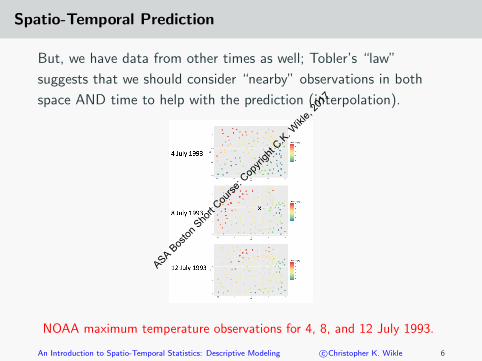
But, we have data from other times as well; Tobler’s “law”
suggests that we should consider “nearby” observations in both
space AND time to help with the prediction (interpolation).
NOAA maximum temperature observations for 4, 8, and 12 July 1993.
An Introduction to Spatio-Temporal Statistics: Descriptive Modeling c©Christopher K. Wikle 6
ASA Bos
ton S
hort C
ourse
: Cop
yrigh
t C.K
. Wikl
e, 20
17
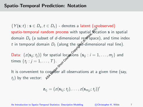
Spatio-Temporal Prediction: Notation
{Y (s; t) : s ∈ Ds , t ∈ Dt} - denotes a latent (unobserved)
spatio-temporal random process with spatial location s in spatial
domain Ds (a subset of d-dimensional real space), and time index
t in temporal domain Dt (along the one-dimensional real line).
Data: {z(sij ; tj)} for spatial locations {sij : i = 1, . . . ,mj} and
times {tj : j = 1, . . . ,T}.
It is convenient to consider all observations at a given time (say,
tj) by the vector:
ztj = (z(s1j ; tj), . . . , z(smj j ; tj))′
An Introduction to Spatio-Temporal Statistics: Descriptive Modeling c©Christopher K. Wikle 7
ASA Bos
ton S
hort C
ourse
: Cop
yrigh
t C.K
. Wikl
e, 20
17

Spatio-Temporal Prediction: Data Model
We represent the data in terms of the latent spatio-temporal
process of interest plus an error:
z(sij ; tj) = Y (sij ; tj) + ε(sij ; tj), i = 1, . . . ,mj ; j = 1, . . . ,T ,
Assumptions:
• {ε(sij ; tj)} - independent and identically distributed mean-zero
observation errors that are independent of Y and have
variance σ2ε
• the errors are assumed to have a normal (Gaussian)
distribution here; ε(sij ; tj) ∼ iid N(0, σ2ε ) (or, we might write
this ε(sij ; tj) ∼ iid Gau(0, σ2ε ))
An Introduction to Spatio-Temporal Statistics: Descriptive Modeling c©Christopher K. Wikle 8
ASA Bos
ton S
hort C
ourse
: Cop
yrigh
t C.K
. Wikl
e, 20
17

Spatio-Temporal Prediction: Goal
We seek to predict the “true” (latent) process at some location
(s0; t0) (for which we might not have data): Y (s0; t0) given all of
the observations {z(sij , tj) : i = 1, . . . ,mj ; j = 1, . . . ,T}.
Consider the linear predictor of the form:
Y (s0; t0) =T∑j=1
mj∑i=1
wij z(sij , tj)
How do we choose these weights?
• they typically reflect Tobler’s “first law of geography”; thecloser an observation is to location (s0; t0), the larger theweight
• this is similar to kernel-weighted regression, but the “optimal”weights (see below) consider spatio-temporal dependencemore directly
An Introduction to Spatio-Temporal Statistics: Descriptive Modeling c©Christopher K. Wikle 9
ASA Bos
ton S
hort C
ourse
: Cop
yrigh
t C.K
. Wikl
e, 20
17

Spatio-Temporal Prediction: Cartoon
Cartoon showing spatio-temporal prediction of latent process Y (s0; t0)
given observations at time t0 and before and after. The solid arrows
depict the prediction weights wij for the various observations.
An Introduction to Spatio-Temporal Statistics: Descriptive Modeling c©Christopher K. Wikle 10
ASA Bos
ton S
hort C
ourse
: Cop
yrigh
t C.K
. Wikl
e, 20
17
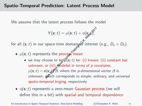
Spatio-Temporal Prediction: Latent Process Model
We assume that the latent process follows the model
Y (s; t) = µ(s; t) + η(s; t),
for all (s; t) in our space-time domain of interest (e.g., Ds × Dt).
• µ(s; t) represents the process mean
• we may choose to let µ(s; t) be: (i) known, (ii) constant but
unknown, or (iii) modeled in terms of p covariates,
µ(s; t) = x(s; t)′β, where the p-dimensional vector β is
unknown, which corresponds to simple, ordinary, and universal
spatio-temporal kriging, respectively
• η(s; t) represents a zero-mean Gaussian process (we will
define this in a bit) with spatial and temporal dependence
An Introduction to Spatio-Temporal Statistics: Descriptive Modeling c©Christopher K. Wikle 11
ASA Bos
ton S
hort C
ourse
: Cop
yrigh
t C.K
. Wikl
e, 20
17
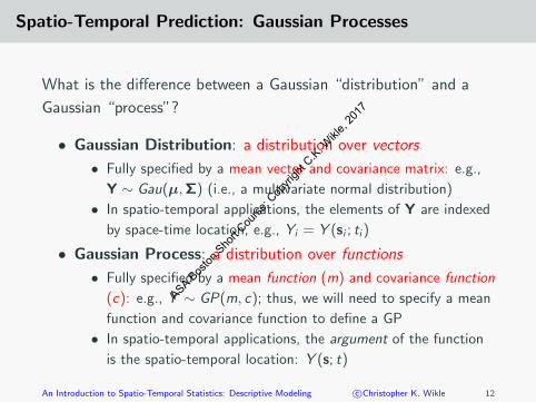
Spatio-Temporal Prediction: Gaussian Processes
What is the difference between a Gaussian “distribution” and a
Gaussian “process”?
• Gaussian Distribution: a distribution over vectors
• Fully specified by a mean vector and covariance matrix: e.g.,
Y ∼ Gau(µ,Σ) (i.e., a multivariate normal distribution)
• In spatio-temporal applications, the elements of Y are indexed
by space-time location, e.g., Yi = Y (si ; ti )
• Gaussian Process: a distribution over functions
• Fully specified by a mean function (m) and covariance function
(c): e.g., Y ∼ GP(m, c); thus, we will need to specify a mean
function and covariance function to define a GP
• In spatio-temporal applications, the argument of the function
is the spatio-temporal location: Y (s; t)
An Introduction to Spatio-Temporal Statistics: Descriptive Modeling c©Christopher K. Wikle 12
ASA Bos
ton S
hort C
ourse
: Cop
yrigh
t C.K
. Wikl
e, 20
17

Spatio-Temporal Prediction: Gaussian Processes
Why GPs?
• A GP is an infinite-dimensional object
• This will allow us to make a prediction anywhere in our
space-time domain (if we know the mean and covariance
functions)
• But, in practice we will only ever need to considerfinite-dimensional distributions; why?
• We only have a finite set of data and are eventually only
interested in a finite set of prediction locations
• Any finite collection of GP random variables has a joint
Gaussian distribution
• This allows us to use the traditional machinery of multivariate
normal distributions and linear mixed models to do calculations
An Introduction to Spatio-Temporal Statistics: Descriptive Modeling c©Christopher K. Wikle 13
ASA Bos
ton S
hort C
ourse
: Cop
yrigh
t C.K
. Wikl
e, 20
17

Spatio-Temporal Prediction: Gaussian Distributions
Technical Review:
Recall the famous result relating joint and conditional Gaussian
random variables:(v
v∗
)∼ Gau
((µ
µ∗
),
(Σ Σ∗Σ′∗ Σ∗∗
))
where E (v) = µ, E (v∗) = µ∗, Σ = cov(v, v), Σ∗ = cov(v, v∗),
and Σ∗∗ = cov(v∗, v∗).
Then,
v∗|v ∼ Gau(µ∗ + Σ′∗Σ−1(v − µ),Σ∗∗ −Σ′∗Σ
−1Σ∗)
An Introduction to Spatio-Temporal Statistics: Descriptive Modeling c©Christopher K. Wikle 14
ASA Bos
ton S
hort C
ourse
: Cop
yrigh
t C.K
. Wikl
e, 20
17

Spatio-Temporal Prediction: Optimal Linear Prediction
Let’s get back to the problem at hand:
Recall we are interested in predicting Y (s0; t0) (i.e., at some
arbitrary location in space-time) given the data
z ≡ (z(s11; t1), . . . , z(smT ; tT ))′. As we mentioned, we are looking
for linear predictors of the form:
Y (s0; t0) =T∑j=1
mj∑i=1
wij z(sij , tj) = w′0z.
Thus, we seek the conditional distribution:
[Y (s0; t0) | z ].
Why not [Z(s0; t0) | z ]?
An Introduction to Spatio-Temporal Statistics: Descriptive Modeling c©Christopher K. Wikle 15
ASA Bos
ton S
hort C
ourse
: Cop
yrigh
t C.K
. Wikl
e, 20
17

Spatio-Temporal Prediction: Optimal Linear Prediction
It helps to rewrite the data model in vector form:
z = Y + ε, ε ∼ Gau(0,Cε)
where Y and ε are ordered in the same way as the data vector z.
Now, cov(Y,Y) ≡ Cy , cov(ε, ε) ≡ Cε, cov(z, z) = Cy + Cε.
In addition, c′0 ≡ cov(Y (s0; t0), z), c0,0 ≡ var(Y (s0; t0)), and X is
the (∑T
j=1mj)× p matrix of known covariates. Then, consider the
joint Gaussian distribution:[Y (s0; t0)
z
]∼ Gau
([x(s0; t0)′
X
]β ,
[c0,0 c′0c0 Cz
]).
An Introduction to Spatio-Temporal Statistics: Descriptive Modeling c©Christopher K. Wikle 16
ASA Bos
ton S
hort C
ourse
: Cop
yrigh
t C.K
. Wikl
e, 20
17

Spatio-Temporal Prediction: Optimal Linear Prediction
Using the joint/conditional Gaussian distribution formula from
before (and, assuming for the moment that β is known; i.e., simple
spatio-temporal kriging) we get
Y (s0; t0) |z ∼ Gau(x(s0; t0)′β+c′0C−1z (z−Xβ) , c0,0−c′0C−1z c0).
An Introduction to Spatio-Temporal Statistics: Descriptive Modeling c©Christopher K. Wikle 17
ASA Bos
ton S
hort C
ourse
: Cop
yrigh
t C.K
. Wikl
e, 20
17
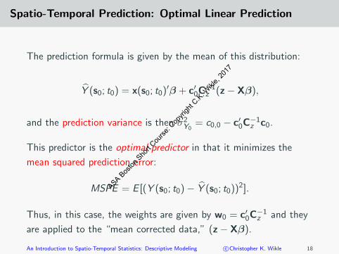
Spatio-Temporal Prediction: Optimal Linear Prediction
The prediction formula is given by the mean of this distribution:
Y (s0; t0) = x(s0; t0)′β + c′0C−1z (z− Xβ),
and the prediction variance is then σ2Y0= c0,0 − c′0C−1z c0.
This predictor is the optimal predictor in that it minimizes the
mean squared prediction error:
MSPE = E [(Y (s0; t0)− Y (s0; t0))2].
Thus, in this case, the weights are given by w0 = c′0C−1z and they
are applied to the “mean corrected data,” (z− Xβ).
An Introduction to Spatio-Temporal Statistics: Descriptive Modeling c©Christopher K. Wikle 18
ASA Bos
ton S
hort C
ourse
: Cop
yrigh
t C.K
. Wikl
e, 20
17

Spatio-Temporal Prediction: Optimal Linear Prediction
Let’s take a closer look at the predictive distribution:
(Note, it is simple to predict at many new locations, say Y0. The
formulas are slightly modified to include matrices for X0, C0 and c0,0.)
An Introduction to Spatio-Temporal Statistics: Descriptive Modeling c©Christopher K. Wikle 19
ASA Bos
ton S
hort C
ourse
: Cop
yrigh
t C.K
. Wikl
e, 20
17
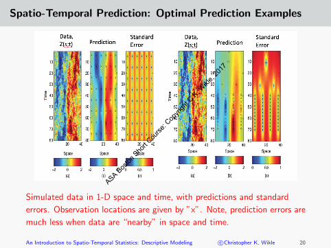
Spatio-Temporal Prediction: Optimal Prediction Examples
Simulated data in 1-D space and time, with predictions and standard
errors. Observation locations are given by ”x”. Note, prediction errors are
much less when data are “nearby” in space and time.
An Introduction to Spatio-Temporal Statistics: Descriptive Modeling c©Christopher K. Wikle 20
ASA Bos
ton S
hort C
ourse
: Cop
yrigh
t C.K
. Wikl
e, 20
17
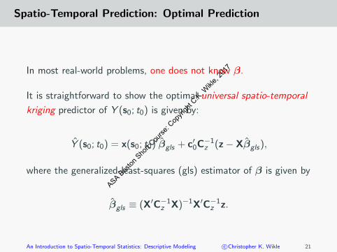
Spatio-Temporal Prediction: Optimal Prediction
In most real-world problems, one does not know β.
It is straightforward to show the optimal universal spatio-temporal
kriging predictor of Y (s0; t0) is given by:
Y (s0; t0) = x(s0; t0)′βgls + c′0C−1z (z− Xβgls),
where the generalized-least-squares (gls) estimator of β is given by
βgls ≡ (X′C−1z X)−1X′C−1z z.
An Introduction to Spatio-Temporal Statistics: Descriptive Modeling c©Christopher K. Wikle 21
ASA Bos
ton S
hort C
ourse
: Cop
yrigh
t C.K
. Wikl
e, 20
17

Spatio-Temporal Prediction: Optimal Prediction
The associated universal spatio-temporal kriging variance is given
by
σ2Y ,uk(s0; t0) = c0,0 − c′0C−1z c0 + κ,
where
κ ≡ (x(s0; t0)− X′C−1z c0)′(X′C−1z X)−1(x(s0; t0)− X′C−1z c0),
represents the additional uncertainty brought to the prediction
(relative to simple kriging) due to the estimation of β.
An Introduction to Spatio-Temporal Statistics: Descriptive Modeling c©Christopher K. Wikle 22
ASA Bos
ton S
hort C
ourse
: Cop
yrigh
t C.K
. Wikl
e, 20
17
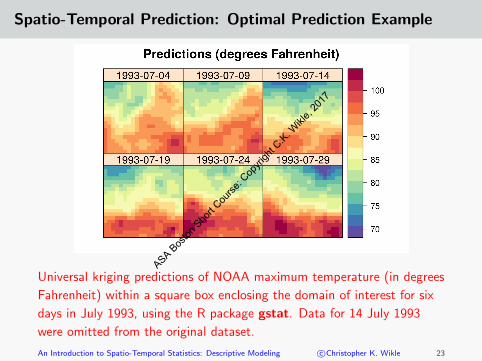
Spatio-Temporal Prediction: Optimal Prediction Example
Universal kriging predictions of NOAA maximum temperature (in degrees
Fahrenheit) within a square box enclosing the domain of interest for six
days in July 1993, using the R package gstat. Data for 14 July 1993
were omitted from the original dataset.
An Introduction to Spatio-Temporal Statistics: Descriptive Modeling c©Christopher K. Wikle 23
ASA Bos
ton S
hort C
ourse
: Cop
yrigh
t C.K
. Wikl
e, 20
17

Spatio-Temporal Prediction: Optimal Prediction Example
Universal kriging standard errors for predictions of NOAA maximum
temperature (in degrees Fahrenheit) within a square box enclosing the
domain of interest for six days in July 1993, using the R package gstat.
Data for 14 July 1993 were omitted from the original dataset.
An Introduction to Spatio-Temporal Statistics: Descriptive Modeling c©Christopher K. Wikle 24
ASA Bos
ton S
hort C
ourse
: Cop
yrigh
t C.K
. Wikl
e, 20
17

Covariance Functions
ASA Bos
ton S
hort C
ourse
: Cop
yrigh
t C.K
. Wikl
e, 20
17

Spatio-Temporal Prediction: Covariance Functions
Recall that we considered the spatio-temporal process as a
Gaussian Process here because we need the covariance function
between ANY space-time locations. This requires that we specify a
mean function (easy) and a covariance function (not so easy).
So far, we assumed that we knew the variances and covariances
that make up Cy , Cε, c0, and c0,0. In the real-world we would
rarely (if ever) know these.
An Introduction to Spatio-Temporal Statistics: Descriptive Modeling c©Christopher K. Wikle 26
ASA Bos
ton S
hort C
ourse
: Cop
yrigh
t C.K
. Wikl
e, 20
17

Spatio-Temporal Prediction: Covariance Functions
Seemingly simple solution: specify covariance functions in terms
of parameters, θ, that can give a covariance between any pairs of
space-time coordinates, and then estimate the parameters (see
below).
In spatio-temporal data analysis, as with spatial statistics, the
specification of these covariance functions becomes one of the
most challenging components of the problem. Why?
• Covariance functions must be positive semi-definite (this
ensures that prediction variances are non-negative!)
• Covariance functions should be realistic (that is, they should
account for realistic dependencies)
An Introduction to Spatio-Temporal Statistics: Descriptive Modeling c©Christopher K. Wikle 27
ASA Bos
ton S
hort C
ourse
: Cop
yrigh
t C.K
. Wikl
e, 20
17

Spatio-Temporal Prediction: Covariance Functions
In practice, classical kriging implementations typically make a
stationarity assumption.
For example, if the random process is assumed to be second-order
(weakly) stationary then it has constant expectation and a
covariance function that can be expressed in terms of the spatial
and temporal lags
c(h ; τ) ≡ c(sij − sk` ; tj − t`), (1)
where h ≡ sij − sk` and τ ≡ tj − t` are the spatial and temporal
lags, respectively.
Recall from our exploratory analyses that if the spatial lag does not
depend on direction (i.e., h = ||h||), we say there is spatial isotropy.
An Introduction to Spatio-Temporal Statistics: Descriptive Modeling c©Christopher K. Wikle 28
ASA Bos
ton S
hort C
ourse
: Cop
yrigh
t C.K
. Wikl
e, 20
17
Spatio-Temporal Prediction: Covariance Functions
Two biggest benefits of the stationarity assumption:
• allows for more parsimonious parameterizations of the
covariance function
• provides pseudo-replication of dependencies at given lags in
space and time, both of which facilitate estimation
The next question is how do we specify (or construct) such valid
covariance functions? Traditionally,
• separable covariance functions
• sums-and-products formulations
• spectral construction
• stochastic partial differential equation solutions
An Introduction to Spatio-Temporal Statistics: Descriptive Modeling c©Christopher K. Wikle 29
ASA Bos
ton S
hort C
ourse
: Cop
yrigh
t C.K
. Wikl
e, 20
17

Spatio-Temporal Prediction: Covariance Functions
Separable Covariance Functions:
c(h; τ) ≡ c(s)(h) · c(t)(τ),
which is valid if both the spatial covariance, c(s)(h), and temporal
covariance c(t)(τ) are valid.
An Introduction to Spatio-Temporal Statistics: Descriptive Modeling c©Christopher K. Wikle 30
ASA Bos
ton S
hort C
ourse
: Cop
yrigh
t C.K
. Wikl
e, 20
17

Spatio-Temporal Prediction: Covariance Functions
There are a large number of classes of valid spatial and temporal
covariance functions in the literature (e.g., the Matern, powered
exponential, and Gaussian classes, to name but a few). For
example, the exponential covariance function is given by
c(t)(τ) = σ2 exp{−τa
},
where σ2 is the variance parameter and a is the dependence
parameter.
Exponential covariance function for time lag, τ ; σ2 = 2.5 and a = 2.
An Introduction to Spatio-Temporal Statistics: Descriptive Modeling c©Christopher K. Wikle 31
ASA Bos
ton S
hort C
ourse
: Cop
yrigh
t C.K
. Wikl
e, 20
17

Spatio-Temporal Prediction: Covariance Functions
Benefit of Separable Covariance Functions:
Separable models help with computation in problems with many
spatial and/or temporal locations (e.g., matrix inverses).
Technical Note:
For example, assume that Z(sij ; tj) is observed at each of mj = m locations and
each time point, j = 1, . . . ,T .
Separability allows us to write: Cz = C(t)z ⊗ C(s)
z , where ⊗ is the Kronecker
product, C(s)z is the m ×m spatial covariance matrix, and C(t)
z is the T × T
temporal covariance matrix.
In this case, C−1z = (C(t)
z )−1 ⊗ (C(s)z )−1, which shows that one only has to take
the inverse of m and T dimensional matrices to get the inverse of the much
larger (mT )× (mT ) matrix.
An Introduction to Spatio-Temporal Statistics: Descriptive Modeling c©Christopher K. Wikle 32
ASA Bos
ton S
hort C
ourse
: Cop
yrigh
t C.K
. Wikl
e, 20
17

Spatio-Temporal Prediction: Covariance Functions
Separable Covariance Functions:
Consider the NOAA maximum temperature dataset. The left panel
below shows a contour plot of the empirical spatio-temporal
covariance function and the right panel shows the product of the
empirical spatial (c(s)(‖h‖; 0)) and temporal (c(t)(0; τ)) marginal
covariance functions. These plots suggest that separability may be
a reasonable assumption for these data.
An Introduction to Spatio-Temporal Statistics: Descriptive Modeling c©Christopher K. Wikle 33
ASA Bos
ton S
hort C
ourse
: Cop
yrigh
t C.K
. Wikl
e, 20
17
Spatio-Temporal Prediction: Covariance Functions
Separability is unusual in spatio-temporal processes; it says that
temporal evolution of the process at a given spatial location does
not depend directly on the process’ temporal evolution at other
locations. That is, separability comes from a lack of
spatio-temporal interaction in Y (·; ·).
What other options do we have to specify S-T covariance
functions?
• Sums and products of covariance functions
• Construction (e.g., spectrally, via Bochner’s Theorem, which
relates the spectral representation to the covariance
representation)
• Solving a stochastic partial differential equation (SPDE)
An Introduction to Spatio-Temporal Statistics: Descriptive Modeling c©Christopher K. Wikle 34
ASA Bos
ton S
hort C
ourse
: Cop
yrigh
t C.K
. Wikl
e, 20
17

Spatio-Temporal Prediction: Covariance Functions
Other Options – Sums and Products of Covariance Functions:
Because the products and sums of valid covariance functions are
valid, we can define:
c(h; τ) ≡ p c(s)1 (h) · c(t)1 (τ) + q c
(s)2 (h) + r c
(t)2 (τ),
for p > 0, q ≥ 0, r ≥ 0, and where c(s)1 (h) and c
(s)2 (h) are valid
spatial covariance functions and c(t)1 (τ) and c
(t)2 (τ) are valid
temporal covariance functions.
In general, it is not clear if realistic processes can be modeled by such
structures. A special case, sometimes known as a “fully symmetric
spatio-temporal covariance function” implies
cov(Y (s; t),Y (s′; t′)) = cov(Y (s; t′),Y (s′; t)),
which is not realistic for many processes.
An Introduction to Spatio-Temporal Statistics: Descriptive Modeling c©Christopher K. Wikle 35
ASA Bos
ton S
hort C
ourse
: Cop
yrigh
t C.K
. Wikl
e, 20
17
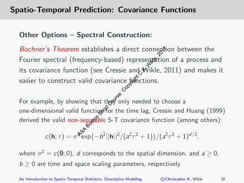
Spatio-Temporal Prediction: Covariance Functions
Other Options – Spectral Construction:
Bochner’s Theorem establishes a direct connection between the
Fourier spectral (frequency-based) representation of a process and
its covariance function (see Cressie and Wikle, 2011) and makes it
easier to construct valid covariance functions.
For example, by showing that they only needed to choose a
one-dimensional valid function for the time lag, Cressie and Huang (1999)
derived the valid non-separable S-T covariance function (among others):
c(h; τ) = σ2 exp{−b2||h||2/(a2τ 2 + 1)}/(a2τ 2 + 1)d/2,
where σ2 = c(0; 0), d corresponds to the spatial dimension, and a ≥ 0,
b ≥ 0 are time and space scaling parameters, respectively.
An Introduction to Spatio-Temporal Statistics: Descriptive Modeling c©Christopher K. Wikle 36
ASA Bos
ton S
hort C
ourse
: Cop
yrigh
t C.K
. Wikl
e, 20
17

Spatio-Temporal Prediction: Covariance Functions
Spectral Construction:
Left: Contour plot of the nonseparable Cressie-Huang covariance function
for d = 1, a = 2, b = 0.2, and σ = 1. Right: Equivalent separable
representation based on the product of the spatial and temporal marginal
correlation functions.
An Introduction to Spatio-Temporal Statistics: Descriptive Modeling c©Christopher K. Wikle 37
ASA Bos
ton S
hort C
ourse
: Cop
yrigh
t C.K
. Wikl
e, 20
17

Spatio-Temporal Prediction: Covariance Functions
Other Options – SPDE-Derived Covariance Functions:
The SPDE approach to deriving spatio-temporal covariance
functions was originally inspired by statistical physics, where
physical equations (PDEs) forced by random processes that
describe advective, diffusive, and decay behavior can be used, in
principle, to describe the second moments of macro-scale processes.
Most famous examples: the ubiquitous Matern class of spatial
covariance functions can be derived from a linear diffusion SPDE
(e.g., Whittle 1962; see Guttorp and Gneiting (2006) for historical
perspective) and the reaction-diffusion model of Heine (1955).
Although these approaches can suggest nonseparable
spatio-temporal covariance functions, only a few special (simple)
models lead to closed forms.An Introduction to Spatio-Temporal Statistics: Descriptive Modeling c©Christopher K. Wikle 38
ASA Bos
ton S
hort C
ourse
: Cop
yrigh
t C.K
. Wikl
e, 20
17

Descriptive Modeling: Part II
(Estimation)
ASA Bos
ton S
hort C
ourse
: Cop
yrigh
t C.K
. Wikl
e, 20
17

Spatio-Temporal Prediction: Estimation
The spatio-temporal covariance models presented above depend on
unknown parameters; these must be estimated from the data.
There is a history in spatial statistics of fitting such models directly
to the empirical estimates (e.g., by using a least squares or
weighted least squares approach; see Cressie 1993, Section 2.6 for
an overview).
In the spatio-temporal context, one typically considers covariance
models and estimates parameters through likelihood-based
methods or through fully Bayesian methods. This follows closely
the approaches in linear mixed model parameter estimation (for an
overview see McCulloch and Searle, 2001).
An Introduction to Spatio-Temporal Statistics: Descriptive Modeling c©Christopher K. Wikle 40
ASA Bos
ton S
hort C
ourse
: Cop
yrigh
t C.K
. Wikl
e, 20
17
Spatio-Temporal Prediction: Estimation
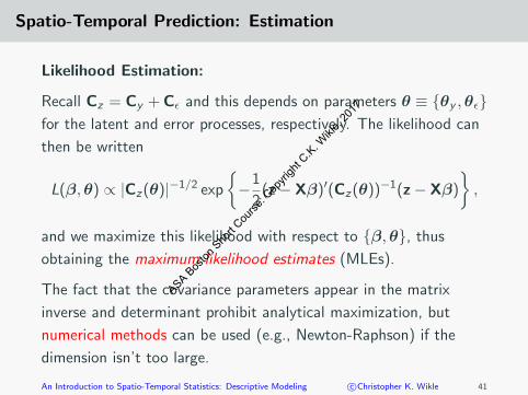
Likelihood Estimation:
Recall Cz = Cy + Cε and this depends on parameters θ ≡ {θy ,θε}for the latent and error processes, respectively. The likelihood can
then be written
L(β,θ) ∝ |Cz(θ)|−1/2 exp
{−1
2(z− Xβ)′(Cz(θ))−1(z− Xβ)
},
and we maximize this likelihood with respect to {β,θ}, thus
obtaining the maximum likelihood estimates (MLEs).
The fact that the covariance parameters appear in the matrix
inverse and determinant prohibit analytical maximization, but
numerical methods can be used (e.g., Newton-Raphson) if the
dimension isn’t too large.
An Introduction to Spatio-Temporal Statistics: Descriptive Modeling c©Christopher K. Wikle 41
ASA Bos
ton S
hort C
ourse
: Cop
yrigh
t C.K
. Wikl
e, 20
17

Spatio-Temporal Prediction: Estimation
Restricted Maximum Likelihood Estimation (REML):
REML considers the likelihood of a linear transformation of the
data vector such that the errors are orthogonal to the Xs that
make up the mean function.
Numerical maximization of the associated likelihood, which is only
a function of the θ parameters, is typically more computationally
efficient than for MLEs (and, conventional wisdom is that the bias
properties of the REML covariance parameter estimates are better
than MLEs for linear mixed models.)
An Introduction to Spatio-Temporal Statistics: Descriptive Modeling c©Christopher K. Wikle 42
ASA Bos
ton S
hort C
ourse
: Cop
yrigh
t C.K
. Wikl
e, 20
17

Spatio-Temporal Prediction: Estimation
Fully (Hierarchical) Bayesian Estimation:
Recall, we can decompose an arbitrary joint distribution in terms of
a hierarchical sequence of conditional distributions and a marginal
distribution, e.g., [A,B,C ] = [A|B,C ][B|C ][C ].
In the context of the general spatio-temporal model,
[z,Y,β,θ] = [z|Y,θ,β][Y|β,θ][β|θ][θ]
= [z|Y,θε][Y|β,θy ][θ][β],
where θ contains all of the variance and covariance parameters
from the data model and the process model.
Note that the first equality is based on the probability
decomposition and the second equality is based on writing
θ = {θε,θy} and assuming the priors on β and θ are independent.
An Introduction to Spatio-Temporal Statistics: Descriptive Modeling c©Christopher K. Wikle 43
ASA Bos
ton S
hort C
ourse
: Cop
yrigh
t C.K
. Wikl
e, 20
17

Spatio-Temporal Prediction: Estimation
Fully (Hierarchical) Bayesian Estimation:
Now, Bayes’ rule gives the posterior distribution
[Y,β,θ|z] ∝ [z|Y,θε][Y|β,θy ][θ][β],
where [z|Y,θε] is the data model and [Y|β,θy ] is the latent
process model. The prior distributions for the parameters [θ] and
[β] are then specified according to the specific choices one makes
for the error and process covariance functions.
In general, the normalizing constant required to fully specify the
posterior distribution is not available analytically and numerical
sampling methods (e.g., Markov chain Monte Carlo, MCMC) must
be used.
Advantage of the Bayesian hierarchical model (BHM) approach:
parameter uncertainty accounted for directlyAn Introduction to Spatio-Temporal Statistics: Descriptive Modeling c©Christopher K. Wikle 44
ASA Bos
ton S
hort C
ourse
: Cop
yrigh
t C.K
. Wikl
e, 20
17
Spatio-Temporal Prediction: Estimation
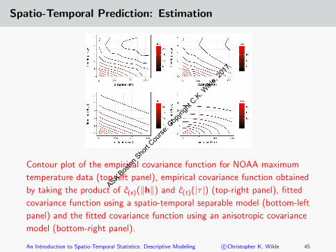
Contour plot of the empirical covariance function for NOAA maximum
temperature data (top-left panel), empirical covariance function obtained
by taking the product of c(s)(‖h‖) and c(t)(|τ |) (top-right panel), fitted
covariance function using a spatio-temporal separable model (bottom-left
panel) and the fitted covariance function using an anisotropic covariance
model (bottom-right panel).
An Introduction to Spatio-Temporal Statistics: Descriptive Modeling c©Christopher K. Wikle 45
ASA Bos
ton S
hort C
ourse
: Cop
yrigh
t C.K
. Wikl
e, 20
17

Descriptive Modeling: Part III
(Basis Functions and Random
Effects Parameterizations)
ASA Bos
ton S
hort C
ourse
: Cop
yrigh
t C.K
. Wikl
e, 20
17

Spatio-Temporal Basis Function and Random Effects Models
Two problems:
• difficulty in working with large spatio-temporal covariance
matrices (e.g., C−1z ) in situations with large numbers of
prediction or observation locations
• realistic covariance structure
Possible solution:
Expand the spatio-temporal process in terms of basis functions and
associated random effects and take advantage of conditional
specifications that a hierarchical modeling framework allows.
An Introduction to Spatio-Temporal Statistics: Descriptive Modeling c©Christopher K. Wikle 47
ASA Bos
ton S
hort C
ourse
: Cop
yrigh
t C.K
. Wikl
e, 20
17
Spatio-Temporal Basis Function and Random Effects Models
One can consider classical linear mixed models from either a
conditional perspective, where one conditions the response on
random effects, or from a marginal perspective, where the random
effects have been averaged out.
Example: in a longitudinal-data-analysis setting, one might allow
there to be subject-specific intercepts or slopes corresponding to a
drug treatment effect over time. The variation in the subject
intercepts and slopes are specified by random effects.
An Introduction to Spatio-Temporal Statistics: Descriptive Modeling c©Christopher K. Wikle 48
ASA Bos
ton S
hort C
ourse
: Cop
yrigh
t C.K
. Wikl
e, 20
17

Spatio-Temporal Basis Function and Random Effects Models
Longitudinal study with two treatments and a control (Verdonck et al. 1998).
• subject level (conditional) inference
• treatment effect (marginal) inference
Key: shared random effects induce dependence!
An Introduction to Spatio-Temporal Statistics: Descriptive Modeling c©Christopher K. Wikle 49
ASA Bos
ton S
hort C
ourse
: Cop
yrigh
t C.K
. Wikl
e, 20
17

Spatio-Temporal Basis Function and Random Effects Models
As in traditional linear mixed models, consider:
z = Y + ε,
Y = Xβ + Φα,
where ε ∼ Gau(0,Cε), and α ∼ Gau(0,Cα).
Alternatively, we can write this conditionally:
z|Y ∼ Gau(Xβ + Φα,Cε),
α ∼ Gau(0,Cα).
Integrating out the random effects (α) we get the marginal
representation:
z ∼ Gau(Xβ,ΦCαΦ′ + Cε).
Thus, averaging across the random effects induces marginal
dependence (e.g., ΦCαΦ′ + Cε versus just Cε).
An Introduction to Spatio-Temporal Statistics: Descriptive Modeling c©Christopher K. Wikle 50
ASA Bos
ton S
hort C
ourse
: Cop
yrigh
t C.K
. Wikl
e, 20
17

Spatio-Temporal Basis Function and Random Effects Models
In the context of spatio-temporal models, we can use this
conditional perspective to specify common random effects that
simplify modeling by either reducing the dimension, simplifying the
conditional dependence structure, or speeding up computation.
Note that in spatial and spatio-temporal cases, we sometimes
include an additional random effect, e.g.,
Y = Xβ + Φα+ ν,
where ν ∼ Gau(0,Cν) and Φ is a matrix of “basis functions”
(broadly speaking).
Before considering this model in more detail, we provide some
basis function intuition.
An Introduction to Spatio-Temporal Statistics: Descriptive Modeling c©Christopher K. Wikle 51
ASA Bos
ton S
hort C
ourse
: Cop
yrigh
t C.K
. Wikl
e, 20
17

Spatio-Temporal Basis Function and Random Effects Models
In recent years, basis-expansion representations have become quite
popular in functional data analysis, nonparametrics, data mining,
and spatial and spatio-temporal statistics. Why? Induced
sparseness, low-rank matrix inverses, non-stationarity,
multi-resolution behavior
In general, we can write
Y (x) ≈p∑
k=1
φk(x)αk ,
where {φk(x), αk : k = 1, . . . , p} are basis functions and the
associated random expansion coefficients (weights) over the
support of x .
For a set of n locations in the domain of x , let Y = (Y (x1), . . . ,Y (xn))′; we
can write the expansion as: Y ≈ Φα.
An Introduction to Spatio-Temporal Statistics: Descriptive Modeling c©Christopher K. Wikle 52
ASA Bos
ton S
hort C
ourse
: Cop
yrigh
t C.K
. Wikl
e, 20
17
Spatio-Temporal Basis Function and Random Effects Models
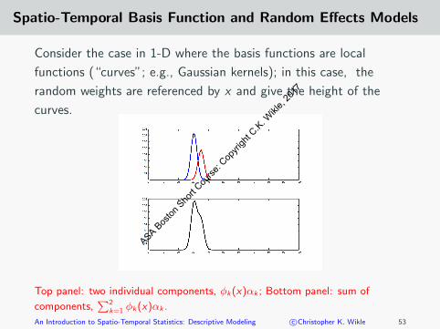
Consider the case in 1-D where the basis functions are local
functions (“curves”; e.g., Gaussian kernels); in this case, the
random weights are referenced by x and give the height of the
curves.
Top panel: two individual components, φk(x)αk ; Bottom panel: sum of
components,∑2
k=1 φk(x)αk .
An Introduction to Spatio-Temporal Statistics: Descriptive Modeling c©Christopher K. Wikle 53
ASA Bos
ton S
hort C
ourse
: Cop
yrigh
t C.K
. Wikl
e, 20
17

Spatio-Temporal Basis Function and Random Effects Models
Consider the same case of local basis functions but with 21 basis
functions:
An Introduction to Spatio-Temporal Statistics: Descriptive Modeling c©Christopher K. Wikle 54
ASA Bos
ton S
hort C
ourse
: Cop
yrigh
t C.K
. Wikl
e, 20
17

Spatio-Temporal Basis Function and Random Effects Models
Now consider the case in 1-D where the basis functions are
“global” curves; in this case, the random weights are not
referenced by x but give the importance of the 8 curves
An Introduction to Spatio-Temporal Statistics: Descriptive Modeling c©Christopher K. Wikle 55
ASA Bos
ton S
hort C
ourse
: Cop
yrigh
t C.K
. Wikl
e, 20
17

Spatio-Temporal Basis Function and Random Effects Models
Finally, consider two realizations of a process with 2-D basis
functions that are “global” surfaces
An Introduction to Spatio-Temporal Statistics: Descriptive Modeling c©Christopher K. Wikle 56
ASA Bos
ton S
hort C
ourse
: Cop
yrigh
t C.K
. Wikl
e, 20
17

Spatio-Temporal Basis Function and Random Effects Models
For modeling spatio-temporal processes we can consider three main
basis function approaches:
• spatio-temporal basis functions: the basis functions are
indexed in space and time and the random effects have no
specific location index
• temporal basis functions: the basis functions are indexed by
time and the random effects are indexed by space
• spatial basis functions: the basis functions are indexed by
space and the random effects are indexed by time
An Introduction to Spatio-Temporal Statistics: Descriptive Modeling c©Christopher K. Wikle 57
ASA Bos
ton S
hort C
ourse
: Cop
yrigh
t C.K
. Wikl
e, 20
17
Spatio-Temporal Basis Function and Random Effects Models
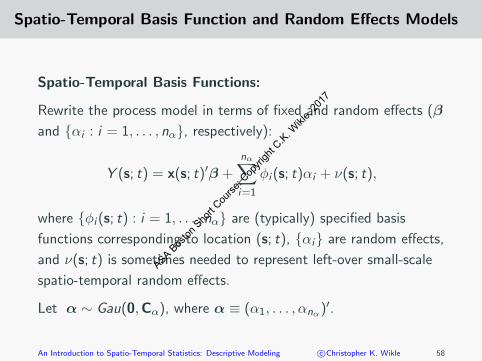
Spatio-Temporal Basis Functions:
Rewrite the process model in terms of fixed and random effects (β
and {αi : i = 1, . . . , nα}, respectively):
Y (s; t) = x(s; t)′β +nα∑i=1
φi (s; t)αi + ν(s; t),
where {φi (s; t) : i = 1, . . . , nα} are (typically) specified basis
functions corresponding to location (s; t), {αi} are random effects,
and ν(s; t) is sometimes needed to represent left-over small-scale
spatio-temporal random effects.
Let α ∼ Gau(0,Cα), where α ≡ (α1, . . . , αnα)′.
An Introduction to Spatio-Temporal Statistics: Descriptive Modeling c©Christopher K. Wikle 58
ASA Bos
ton S
hort C
ourse
: Cop
yrigh
t C.K
. Wikl
e, 20
17

Spatio-Temporal Basis Function and Random Effects Models
Note, we are interested in the Y -process at ny spatio-temporal
locations, which we denote by the vector Y.
The process model then becomes
Y = Xβ + Φα+ ν,
where the ith column of the ny × nα matrix Φ corresponds to the
ith basis function, φi (·; ·), at all of the spatio-temporal locations
ordered as given in Y, and the vector ν also corresponds to the
spatio-temporal ordering given in Y such that ν ∼ Gau(0,Cν).
An Introduction to Spatio-Temporal Statistics: Descriptive Modeling c©Christopher K. Wikle 59
ASA Bos
ton S
hort C
ourse
: Cop
yrigh
t C.K
. Wikl
e, 20
17
Spatio-Temporal Basis Function and Random Effects Models
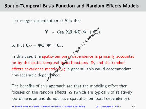
The marginal distribution of Y is then
Y ∼ Gau(Xβ,ΦCαΦ′ + Cν),
so that CY = ΦCαΦ′ + Cν .
In this case, the spatio-temporal dependence is primarily accounted
for by the spatio-temporal basis functions, Φ, and the random
effects covariance matrix Cα; in general, this could accommodate
non-separable dependence.
The benefits of this approach are that the modeling effort then
focuses on the random effects, α (which are typically of relatively
low dimension and do not have spatial or temporal dependence).
An Introduction to Spatio-Temporal Statistics: Descriptive Modeling c©Christopher K. Wikle 60
ASA Bos
ton S
hort C
ourse
: Cop
yrigh
t C.K
. Wikl
e, 20
17
Spatio-Temporal Basis Function and Random Effects Models
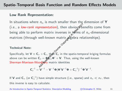
Low Rank Representation:
In situations where nα is much smaller than the dimension of Y
(i.e., a low-rank representation), then obvious benefits come from
being able to perform matrix inverses in terms of nα-dimensional
matrices (through well-known matrix algebra relationships).
Technical Note:
Specifically, let V ≡ Cν + Cε, then Cz in the spatio-temporal kriging formulas
above can be written Cz = ΦΣαΦ′ + V. Thus, using the well-known
Sherman-Morrison-Woodbury matrix identities
C−1z = V−1 − V−1Φ(Φ′V−1Φ + C−1
α )−1Φ′V−1.
If V and Cα (or C−1α ) have simple structure (i.e., sparse) and nα � nY , then
this inverse is easy to calculate.
An Introduction to Spatio-Temporal Statistics: Descriptive Modeling c©Christopher K. Wikle 61
ASA Bos
ton S
hort C
ourse
: Cop
yrigh
t C.K
. Wikl
e, 20
17

Spatio-Temporal Basis Function and Random Effects Models
It is important to note that even in the full-rank (nα equal to the
dimension of Y) and over-complete (nα larger than the dimension
of Y) cases, there can still be dramatic computational benefits
through induced sparsity in Cα and efficient matrix multiplication
routines that utilize multi-resolution algorithms.
In addition, such implementations typically assume that ν = 0 and
are often orthonormal, so that Φ Φ′ = I, which simplifies
calculation significantly.
Finally, we note that specific basis functions and methodologies
take advantage of other properties of the various matrices; e.g.,
sparse structure on the random effects covariance matrix, Cα, or
the random effects precision matrix, C−1α .
An Introduction to Spatio-Temporal Statistics: Descriptive Modeling c©Christopher K. Wikle 62
ASA Bos
ton S
hort C
ourse
: Cop
yrigh
t C.K
. Wikl
e, 20
17

Spatio-Temporal Basis Function and Random Effects Models
Predictions of NOAA maximum temperature for six days spanning the
temporal window of the data, 1-July-1993 – 20-July-2003 using
spatio-temporal bi-square basis functions implemented in the FRK (fixed
rank kriging) R package.An Introduction to Spatio-Temporal Statistics: Descriptive Modeling c©Christopher K. Wikle 63
ASA Bos
ton S
hort C
ourse
: Cop
yrigh
t C.K
. Wikl
e, 20
17

Spatio-Temporal Basis Function and Random Effects Models
Prediction standard errors of NOAA maximum temperature for six days
spanning the temporal window of the data, 1-July-1993 – 20-July-2003
using spatio-temporal bi-square basis functions implemented in the FRK
(fixed rank kriging) R package.An Introduction to Spatio-Temporal Statistics: Descriptive Modeling c©Christopher K. Wikle 64
ASA Bos
ton S
hort C
ourse
: Cop
yrigh
t C.K
. Wikl
e, 20
17

Spatio-Temporal Basis Function and Random Effects Models
An Introduction to Spatio-Temporal Statistics: Descriptive Modeling c©Christopher K. Wikle 65
ASA Bos
ton S
hort C
ourse
: Cop
yrigh
t C.K
. Wikl
e, 20
17

Spatio-Temporal Basis Function and Random Effects Models
Random Effects with Temporal Basis Functions:
We can also express the spatio-temporal random process in terms
of temporal basis functions and spatially-indexed random effects
Y (s; t) = x(s; t)′β +nα∑i=1
φi (t)αi (s) + ν(s; t),
where {φi (t) : i = 1, . . . , nα; t ∈ Dt} are temporal basis functions
and αi (s) are spatially-indexed random effects.
In this case, one could model {αi (s)} using the methods from
spatial statistics. That is, either nα separate spatial processes, or
an nα-dimensional multivariate spatial process (see Cressie and
Wikle, 2011, Ch. 4).
An Introduction to Spatio-Temporal Statistics: Descriptive Modeling c©Christopher K. Wikle 66
ASA Bos
ton S
hort C
ourse
: Cop
yrigh
t C.K
. Wikl
e, 20
17
Spatio-Temporal Basis Function and Random Effects Models
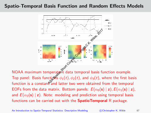
NOAA maximum temperature data temporal basis function example.
Top panel: Basis functions φ1(t), φ2(t), and φ3(t), where the first basis
function is a constant and latter two were obtained from the temporal
EOFs from the data matrix. Bottom panels: E (α0(s) | z),E (α1(s) | z),
and E (α2(s) | z). Note: modeling and prediction using temporal basis
functions can be carried out with the SpatioTemporal R package.
An Introduction to Spatio-Temporal Statistics: Descriptive Modeling c©Christopher K. Wikle 67
ASA Bos
ton S
hort C
ourse
: Cop
yrigh
t C.K
. Wikl
e, 20
17

Spatio-Temporal Basis Function and Random Effects Models
Random Effects with Spatial Basis Functions
We can also express the spatio-temporal random process in terms
of spatial basis functions and temporally-indexed random effects
Y (s; t) = x(s; t)′β +nα∑i=1
φi (s)αt(i) + ν(s; t),
where {φi (s) : i = 1, . . . , nα; s ∈ Ds} are spatial basis functions
and αt(i) are temporal random effects.
The modeling focus is then on modeling the random temporal
effects vectors, αt ≡ (αt(1), . . . , αt(nα))′.
An Introduction to Spatio-Temporal Statistics: Descriptive Modeling c©Christopher K. Wikle 68
ASA Bos
ton S
hort C
ourse
: Cop
yrigh
t C.K
. Wikl
e, 20
17

Spatio-Temporal Basis Function and Random Effects Models
If the αt vectors are independent in time, then the marginal
dependence structure of {Y (s; t)} is typically unrealistic.
Interesting spatio-temporal dependence arises when these effects
are dependent; such models are simplified by assuming conditional
temporal dependence (dynamics!), as we will see in the next
section when we talk about dynamical representations of
spatio-temporal processes.
An Introduction to Spatio-Temporal Statistics: Descriptive Modeling c©Christopher K. Wikle 69
ASA Bos
ton S
hort C
ourse
: Cop
yrigh
t C.K
. Wikl
e, 20
17
Spatio-Temporal Basis Function and Random Effects Models
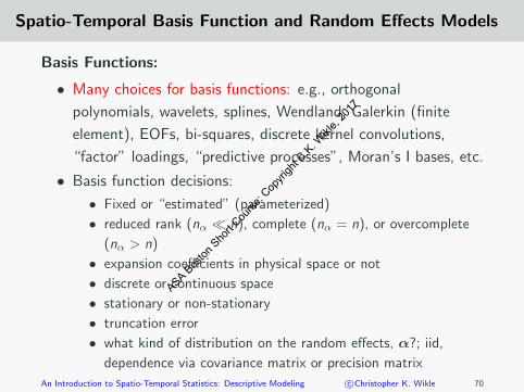
Basis Functions:
• Many choices for basis functions: e.g., orthogonal
polynomials, wavelets, splines, Wendland, Galerkin (finite
element), EOFs, bi-squares, discrete kernel convolutions,
“factor” loadings, “predictive processes”, Moran’s I bases, etc.
• Basis function decisions:
• Fixed or “estimated” (parameterized)
• reduced rank (nα � n), complete (nα = n), or overcomplete
(nα > n)
• expansion coefficients in physical space or not
• discrete or continuous space
• stationary or non-stationary
• truncation error
• what kind of distribution on the random effects, α?; iid,
dependence via covariance matrix or precision matrix
An Introduction to Spatio-Temporal Statistics: Descriptive Modeling c©Christopher K. Wikle 70
ASA Bos
ton S
hort C
ourse
: Cop
yrigh
t C.K
. Wikl
e, 20
17

Spatio-Temporal Basis Function and Random Effects Models
There is very little guidance on which bases or representation to
select!
• people have their favorites and there is a lot of dogma
• practical experience and recent research suggests that in most
cases with just spatial data, it probably doesn’t matter too
much (Bradley et al. 2016)
• in dynamical spatio-temporal model settings, the mechanistic
process can sometimes suggest an appropriate basis set
An Introduction to Spatio-Temporal Statistics: Descriptive Modeling c©Christopher K. Wikle 71
ASA Bos
ton S
hort C
ourse
: Cop
yrigh
t C.K
. Wikl
e, 20
17

Spatio-Temporal Basis Function and Random Effects Models
Confounding:
It is important to mention potential confounding that can occur
between the fixed effects and random effects in dependence
models. This can be particularly important when one is interested
in inference on the β (fixed effects) parameters.
Consider the general mixed-effects representation
Y = Xβ + Φα+ ν, ν ∼ N(0,Cν).
Although the columns of Φ are basis functions, they are indexed in
space and time just as the columns of X.
An Introduction to Spatio-Temporal Statistics: Descriptive Modeling c©Christopher K. Wikle 72
ASA Bos
ton S
hort C
ourse
: Cop
yrigh
t C.K
. Wikl
e, 20
17

Spatio-Temporal Basis Function and Random Effects Models
Confounding:
It is quite possible then that, depending on the structure of the
columns in these two matrices, the random effects can be
confounded with the fixed effects similar to how extreme
collinearity can affect the estimation of fixed effects in traditional
regression.
As with collinearity, if the columns of Φ and X are linearly
independent, then there is no worry from confounding.
This has led to mitigation strategies that tend to restrict the
random effects by selecting basis functions in Φ that are
orthogonal to the column space of X (or, approximately so); see
Hanks et al. (2015) for an overview.
An Introduction to Spatio-Temporal Statistics: Descriptive Modeling c©Christopher K. Wikle 73
ASA Bos
ton S
hort C
ourse
: Cop
yrigh
t C.K
. Wikl
e, 20
17

Descriptive Modeling: Part IV
(Non-Gaussian Data Models with
Latent Gaussian Processes)
ASA Bos
ton S
hort C
ourse
: Cop
yrigh
t C.K
. Wikl
e, 20
17

Non-Gaussian Data and Latent Gaussian Processes
The discussion presented so far has assumed Gaussian error and
random-effects distributions.
Many spatio-temporal problems of interest deal with distinctly
non-Gaussian data (e.g., counts, binary responses, extreme-value
distributions).
One of the most useful aspects of the hierarchical modeling
paradigm is that it allows one to accommodate fairly easily
non-Gaussian data models, so long as the observations are
conditionally independent (e.g., as with Generalized Linear Mixed
Models (GLMMs) and Generalized Additive Models (GAMs)).
An Introduction to Spatio-Temporal Statistics: Descriptive Modeling c©Christopher K. Wikle 75
ASA Bos
ton S
hort C
ourse
: Cop
yrigh
t C.K
. Wikl
e, 20
17

Non-Gaussian Data and Latent Gaussian Processes
As an example, consider the data model
z(s; t)|Y (s; t), γ ∼ ind . EF (Y (s; t), γ),
where EF corresponds to a distribution from the exponential family
with scale parameter γ and mean Y (s; t).
Then, we consider a transformation of the mean response modeled
in terms of fixed and random effects,
g(Y (s; t)) = x(s; t)′β + η(s; t), (2)
where g(·) is a specified monotonic link function, x(s; t) is a
p-dimensional vector of covariates for spatial location s and time t,
and η(s; t) is a spatio-temporal GP.An Introduction to Spatio-Temporal Statistics: Descriptive Modeling c©Christopher K. Wikle 76
ASA Bos
ton S
hort C
ourse
: Cop
yrigh
t C.K
. Wikl
e, 20
17
Non-Gaussian Data and Latent Gaussian Processes
Note that the latent spatio-temporal GP can be modeled in terms
of spatio-temporal covariances, basis function expansions (e.g.,
GAMs), or dynamic spatio-temporal processes (as we will discuss
in the next part of the course).
The same modeling issues associated with this latent Gaussian
spatio-temporal process are present here as with the Gaussian data
case, but estimation is typically more complicated given the
non-Gaussian data model.
An Introduction to Spatio-Temporal Statistics: Descriptive Modeling c©Christopher K. Wikle 77
ASA Bos
ton S
hort C
ourse
: Cop
yrigh
t C.K
. Wikl
e, 20
17

Non-Gaussian Data and Latent Gaussian Processes
As an illustration, a simple model involving spatio-temporal count
data could be represented by
zt |Yt ∼ ind . Poi(Yt),
log(Yt) = Xtβ + Φtα+ νt ,
where zt is an mt × 1 data vector of counts at mt spatial
locations, Yt represents the latent spatio-temporal mean process at
mt locations, Φt is an mt × nα matrix of spatio-temporal basis
functions, and the associated random coefficients are modeled as
α ∼ Gau(0,Cα), with small-scale error term νt ∼ Gau(0, σ2νI).
An Introduction to Spatio-Temporal Statistics: Descriptive Modeling c©Christopher K. Wikle 78
ASA Bos
ton S
hort C
ourse
: Cop
yrigh
t C.K
. Wikl
e, 20
17

Non-Gaussian Data and Latent Gaussian Processes:
Estimation
Implicit in the estimation associated with the linear Gaussian
spatio-temporal model discussed previously is that the covariance
and fixed effects parameters can be estimated more easily when we
marginalize out the latent Gaussian spatio-temporal process.
More generally, we represent this by integrating out the random
effects,
[z|θ,β] =
∫[z|Y,θ][Y|θ,β]dY.
For linear Gaussian mixed models, this can be done analytically;
this is not true for non-Gaussian data models.
An Introduction to Spatio-Temporal Statistics: Descriptive Modeling c©Christopher K. Wikle 79
ASA Bos
ton S
hort C
ourse
: Cop
yrigh
t C.K
. Wikl
e, 20
17
Non-Gaussian Data and Latent Gaussian Processes:
Estimation
The integral in the marginal likelihood given above can be solved
numerically in principle, in which case one can estimate the
relatively few fixed effects and covariance parameters (θ,β)
through usual numerical methods (e.g., Newton-Raphson).
However, this is complicated in practice for spatio-temporal models
by the high-dimensionality of the integral (e.g., recall that Y is an
(∑T
j=1mt)-dimensional vector).
Traditional approaches to this problem are facilitated by the usual
conditional independence assumption in the data model and by
exploiting the latent Gaussian nature of the random effects.
An Introduction to Spatio-Temporal Statistics: Descriptive Modeling c©Christopher K. Wikle 80
ASA Bos
ton S
hort C
ourse
: Cop
yrigh
t C.K
. Wikl
e, 20
17

Non-Gaussian Data and Latent Gaussian Processes:
Estimation
Estimation approaches include methods such as quasi-likelihood,
generalized estimating equations, pseudo-likelihood, penalized
quasi-likelihood and Bayesian methods.
Although these methods can be used successfully in the
spatio-temporal context (e.g., the use of penalized quasi-likelihood
(PQL) in estimating GAMs), there has been much more focus on
Bayesian estimation approaches for spatio-temporal models in the
literature (e.g., Bayesian hieararchical models, Integrated Nested
Laplace Approximations (INLA)).
Regardless, some type of approximation is needed for all of these
methods (approximating integrals, approximating the models,
approximating the posterior distribution). [For examples, see the
mgcv and INLA R packages]An Introduction to Spatio-Temporal Statistics: Descriptive Modeling c©Christopher K. Wikle 81
ASA Bos
ton S
hort C
ourse
: Cop
yrigh
t C.K
. Wikl
e, 20
17

Non-Gaussian Data and Latent Gaussian Processes: Example
Log intensity of Carolina Wren BBS counts in Missouri on a grid for t =
1 (1994) and t = 21 (2014). The log of the observed count is shown in
circles using the same color scale. This was fit using a Poisson data
model and GAM basis functions in the mgcv R package.
An Introduction to Spatio-Temporal Statistics: Descriptive Modeling c©Christopher K. Wikle 82
ASA Bos
ton S
hort C
ourse
: Cop
yrigh
t C.K
. Wikl
e, 20
17

Non-Gaussian Data and Latent Gaussian Processes: Example
Standard error of log intensity of Carolina Wren BBS counts in Missouri
on a grid for t = 1 (1994) and t = 21 (2014). The log of the observed
count is shown in circles using the same color scale. This was fit using a
Poisson data model and GAM basis functions in the mgcv R package.
An Introduction to Spatio-Temporal Statistics: Descriptive Modeling c©Christopher K. Wikle 83
ASA Bos
ton S
hort C
ourse
: Cop
yrigh
t C.K
. Wikl
e, 20
17

Recap
• We focused here on so-called “descriptive” methods for
spatio-temporal prediction; that is, methods that are
concerned with modeling first-order and second-order
dependencies, with the primary goal of performing prediction
in space and time (although, parameter inference is covered in
this context as well).
• A big challenge with these methods is the realistic
specification of valid spatio-temporal covariance functions.
An Introduction to Spatio-Temporal Statistics: Descriptive Modeling c©Christopher K. Wikle 84
ASA Bos
ton S
hort C
ourse
: Cop
yrigh
t C.K
. Wikl
e, 20
17
Recap
• Another challenge is related to the curse-of-dimensionality in
these models.
• Both the dimensionality challenge and the realism challenge
necessitate the consideration of random effects that are
random coefficients in a basis expansion.
• We also considered how it is fairly straightforward to extend
these modeling approaches to non-Gaussian data models, so
long as the data is independent conditional upon a latent
Gaussian spatio-temporal process (although,
computation/estimation is more difficult).
An Introduction to Spatio-Temporal Statistics: Descriptive Modeling c©Christopher K. Wikle 85
ASA Bos
ton S
hort C
ourse
: Cop
yrigh
t C.K
. Wikl
e, 20
17

Next
• One of the most challenging aspects of characterizing the
spatio-temporal dependence structure, either in the
covariance-based perspective or the basis function perspective,
is the ability to model realistically the interactions that occur
across time and space in most real-world processes.
• That is, most processes are best described by spatial fields
that change through time according to “rules” that govern
the behavior. That is, they represent some stochastic
dynamical system.
• As we will see in the next part of the course, spatio-temporal
models that explicitly account for these dynamics offer the
benefit of providing more realistic models in general, are
better for forecasting, and can simplify model construction
and estimation through conditioning.An Introduction to Spatio-Temporal Statistics: Descriptive Modeling c©Christopher K. Wikle 86
ASA Bos
ton S
hort C
ourse
: Cop
yrigh
t C.K
. Wikl
e, 20
17