Energy Procedia

Energy Procedia 00 (2013) 000–000

www.elsevier.com/locate/procedia

2013 International Conference on Alternative Energy in Developing Countries and

Emerging Economies

Wind Energy Projection for the Philippines Based on Climate

Change Modeling

Angeli Silanga,c,*

, Sherdon Niño Uyb, Julie Mae Dado

b, Faye Abigail Cruz

b,

Gemma Narismab,d

, Nathaniel Libatiquea,c

, Gregory Tangonana

aAteneo Innovation Center, Ateneo de Manila University, Quezon City 1108, Philippines bManila Observatory, Quezon City 1108, Philippines

c Electronics, Computer, and Communications Engineering Dept., Ateneo de Manila University, Quezon City 1108,Philippines d Atmospheric Science Program, Dept. of Physics, Ateneo de Manila University, Quezon City 1108,Philippines

Abstract

To complement the existing method of wind energy assessment, this study presents wind energy projection by

downscaling a regional climate model, RegCM3, which is also used in predicting rainfall and temperature changes,

and using a conversion method using the Weibull distribution. A couple of papers which used long-term predicting

models focused on two regions, China and the US High Plains, show a decrease of about 14% and 7%-17%

respectively in wind power density due to global warming over the next century. This paper focuses on a smaller grid

size of 10 km x 10 km to concentrate on a specific wind farm in Pililla, Rizal, Philippines which is considered as a

commercially feasible site by wind developers. Wind energy projection that considers the effects of climate change

for the expected period of operation of 25 years is used because this gives wind developers an outlook on the power

production during the wind farm's lifetime and would contribute in determining the wind farm’s potential for

financial returns. Percentage difference of wind power density between the baseline period of 2008-2012 and five-

year projection periods from 2013-2037 are presented. Contrary to the results of studies in China and western US, the

results of this research show that there is an average five-year period increase of 6% in wind power density in Pililla,

Rizal over the next 25 years.

© 2013 Published by Elsevier Ltd. Selection and/or peer-review under responsibility of the Research

Center in Energy and Environment, Thaksin University.

Keywords: wind energy assessment, climate change, wind projection

* Corresponding author. Tel.: +63-908-869-4416; fax: +63-2-426-5436

E-mail address: angelisilang@alumni.ateneo.edu

2 Angeli Silang et al. / Energy Procedia 00 (2013) 000–000

1. Introduction

The step to move toward cleaner sources of energy has been driven by the noticeable changes in

climate due to global warming. “Going green” by preferring wind energy is one of society’s approaches to

combat climate change. However, wind energy is very much dependent on the wind and monsoons, which

are also affected by climate change. With this cycle where wind energy is a solution for climate change

but climate change could affect wind energy resource, this paper attempts to answer the following

question: How would climate change affect the future of the wind industry?

In China and the United States, wind energy projection studies using climate models were conducted.

Ren [1] used eight regional climate models and concludes that there is a decrease in wind power density

by approximately 14% from 2071 to 2100 in China. For US Western High Plains, Greene et al. [2]

presents in his paper that there will be a decrease of 7% to 17% for the years 2040-2070 when using the

North American Climate Change Assessment Program (NARCCAP) model.

A study by National Renewable Energy Laboratory (NREL) [3] shows that the Philippines has a wind

potential installed capacity of 76.6 GW. Because of this high potential of wind energy in the country,

wind energy developers are interested in commercial wind energy in the Philippines. Most of the projects

of these wind energy developers are in the northern portion of the Philippines, where the Northeast

Monsoon is expected to provide good wind energy yield. There are also other areas in the Philippines that

also show favorable wind potential such as Guimaras and Rizal.

Different from studies in China and US Western High Plains, this paper uses a smaller resolution of 10

km x 10 km grid to focus on a location with a potential for a commercial wind farm operation in Pililla,

Rizal, Philippines.

2. Projected wind results

The work uses the International Centre for Theoretical Physics (ICTP) Regional Climate Model

version 3 (RegCM3) [4] to make projections for the wind fields at Pililla, Rizal. This model is a

hydrostatic model that uses finite differencing method. The wind fields are determined by calculating the

following momentum equations:

uFuFvfp

xx

p

pp

RTmp

up

y

mvup

x

muupm

t

up

VH

t

v

*

*

*

****

2*

/

//

(1)

where u and v are the eastward and northward component of wind velocity, Tv is virtual temperature, ϕ

represents geopotential height, f is the coriolis parameter, R is the gas constant for dry air, m is the map

scale factor. FH and FV are the horizontal and vertical diffusion, respectively. In Eq. (1), , and *p

are defined by these relations: )/()( tst pppp , dtd / and ts ppp * where p is the

pressure, ps is the surface pressure and pt is a specified constant top pressure.

Similar to Eq. (1), the north-south wind vectors are governed by the following equation:

vFvFufpyy

p

tpp

RTmp

up

y

mvvp

x

muvpm

t

vpVH

v

**

*

****

2*

/

//

Angeli Silang et al. / Energy Procedia 00 (2013) 000–000 3

where all expressions are the same with Eq. (1).

Since the Philippines is located at the lower latitudes, the RegCM3 is configured to use the Normal

Mercator projection. The land surface physics is represented in the model with Biosphere-Atmosphere

Transfer Scheme (BATS). Initial and boundary conditions for the near-present and projection simulations

of the model are from the 20C3M experiment and the A1B scenario run of the European Centre/Hamburg

5 (ECHAM5) global climate model. The A1B scenario pertains to a world where economic development

continues at its current pace but mitigation measures are being implemented.

A relatively coarse spatial resolution of 40 km x 40 km over the Philippine domain is simulated.

Results from this run are used to provide boundary conditions for another run at finer resolution of 10 km

x 10 km over the region of interest. The grid closest to Pililla, with approximate coordinates of

14.4773N, 121.366E (WGS84), is processed to obtain the projected wind vectors. RegCM3 results for

Pililla, Rizal at heights 10 m and 110.8 m from 2008-2037 are used in this research.

Villafuerte and Narisma [5] published climate change studies on temperature and rainfall for the

Philippines using RegCM3. The results of which have also been used for climate research in areas such

as Metro Manila, Albay, Leyte, and Bohol. A recent study by Villafuerte [6] on Southwest Monsoon

showed the ability of the model to capture the main features of the prevailing wind flow over the

Philippines with ERA-40 dataset.

In this work, RegCM3 is verified with the Philippine Atmospheric, Geophysical & Astronomical

Services Administration (PAGASA) Tanay station observations for the years of 2000-2005 since it is the

nearest station. While it is preferred for wind energy developers to verify the model with measured data at

height levels between 40 m to 100 m, the model was verified with the available 10-m above ground level

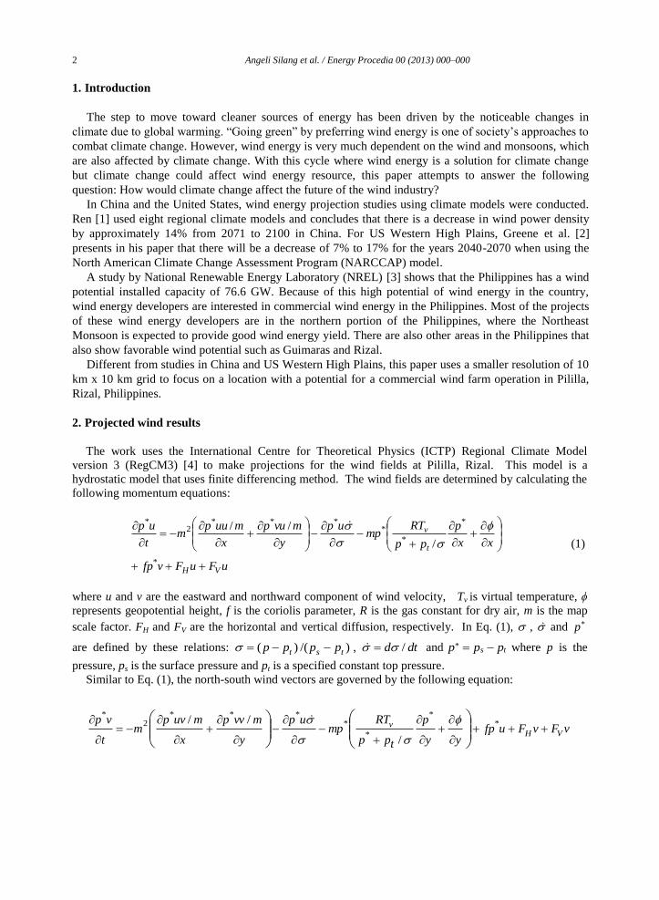
(AGL) PAGASA Tanay data instead. The PAGASA Tanay station is located 12 km north of the 10 km x

10 km grid for Pililla as shown in the topographic map in Fig. 1. As can be seen in the map, there are no

mountain ridges in between Tanay weather station and Pililla. The proximity of the weather station and

the absence of obstruction to the wind flow allow for the verification of the model for Pililla using

observed measurements in Tanay weather station.

Fig. 1. Location of PAGASA Tanay weather station in relation to Pililla 10 km x 10 km grid.

4 Angeli Silang et al. / Energy Procedia 00 (2013) 000–000

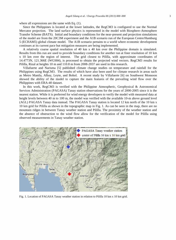
Fig. 2. Histograms of wind speed during the Northeast Monsoon from October to April measured at Tanay PAGASA station and RegCM3 results at 10 m AGL from year 2000 to 2005.

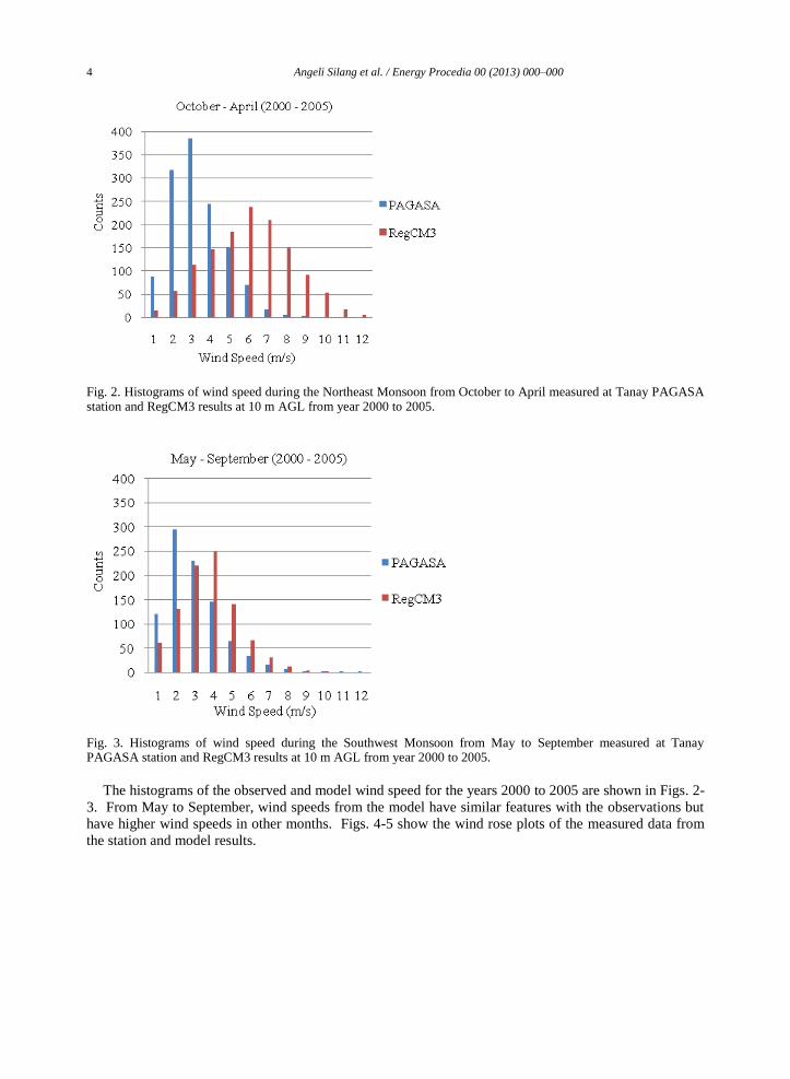
Fig. 3. Histograms of wind speed during the Southwest Monsoon from May to September measured at Tanay PAGASA station and RegCM3 results at 10 m AGL from year 2000 to 2005.

The histograms of the observed and model wind speed for the years 2000 to 2005 are shown in Figs. 2-

3. From May to September, wind speeds from the model have similar features with the observations but

have higher wind speeds in other months. Figs. 4-5 show the wind rose plots of the measured data from

the station and model results.

Angeli Silang et al. / Energy Procedia 00 (2013) 000–000 5

Fig. 4. Wind rose from Tanay PAGASA station for the period 2000-2005 at 10 m AGL.

Fig. 5. Wind rose from RegCM3 results for Tanay station for the period 2000-2005 at 10 m AGL.

Comparing Figs. 4 and 5, it is evident that the model is able to reproduce the general NE direction of

the winds but it is unable to replicate the Easterlies in the observations. It also reflects that the model

generates higher wind speeds than measurements at Tanay station.

Since RegCM3 is developed for regional climate studies, e.g. over areas encompassing the Southeast

Asian region, there is a limitation in its ability to model features at very fine resolutions. Because it is a

hydrostatic model, a spatial resolution lower than 10 km cannot be used in downscaling. Hence, it cannot

simulate micrometeorology. Topography inputs are also approximated to a single value for each grid

point.

The model, however, is able to simulate the overall wind patterns, including the transition from the

Southwest Monsoon season to the Northeast Monsoon season as reflected in the shifting of wind direction

and strengthening of wind magnitude in the global wind data sets [6].

6 Angeli Silang et al. / Energy Procedia 00 (2013) 000–000

3. Conversion model

The model for the conversion of the wind speed projection to wind power density and energy

production is based on the procedures done in wind energy assessment. This model has four parts: a)

interpolation of wind speed to hub height, b) sorting wind speed based on wind direction, c) computing

for wind power density, and d) computing for energy production and capacity factor.

In some cases, part b) is not included in the conversion of wind values to wind energy production

because it is assumed that the use of unimodal Weibull distribution is enough. Sorting wind values based

on wind direction is employed in this model to provide a more accurate probability density function in

case a bimodal distribution is required.

Parts c) and d) provide the equations for wind power density, wind energy production, and capacity

factor which are indicators of whether a site would produce enough wind energy for a commercial wind

farm.

3.1. Interpolation of wind speed to hub height

Since power curves of wind turbines are based on wind speeds at the hub height of the turbine, it is

important to have wind data at this height to determine wind power density and energy production. Data

for the hub height may be extrapolated or interpolated using the wind data at other height levels. There

are two ways to extrapolate or interpolate wind data, one is through the power law and the other is

through logarithmic law. According to P. Gipe [7], power law may be less scientific but more

conservative compared to logarithmic law. Power law is preferred since no information about the surface

roughness of the site is provided, and thus, logarithmic cannot be applied. Moreover, in a paper by Ray et

al. [8], they observed that the accuracy of power law is comparable to the accuracy of logarithmic law. To

interpolate wind speed at the turbine’s hub height, or at any specific height, the power law is used:

refref z

z

v

v (2)

where v is the wind speed at height z, vref is the wind speed at the reference height zref, and α is the power

law exponent [9].

3.2. Sorting wind speed based on wind direction

Usually, the strength of the wind is different for each wind direction. The wind coming from a

particular direction could have a higher wind speed than the wind coming from the opposite direction.

Since the Philippines has two wind seasons, Northeast Monsoon (amihan) from October to April and

Southwest Monsoon (habagat) from May to September, wind speed is categorized based on the direction

of the wind. The two bins have a 180-degree range of values with the center of one bin as the

predominant wind.

After the data is categorized according to the wind direction bins, which also refers to wind seasons,

Weibull distribution is then fitted to the two sets of data.

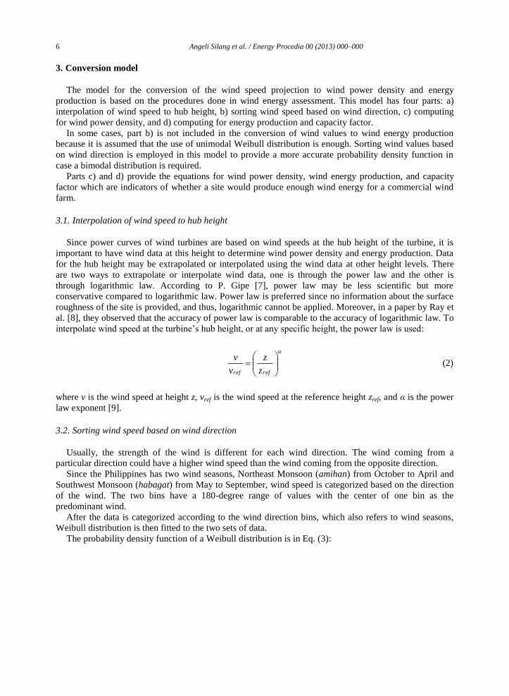
The probability density function of a Weibull distribution is in Eq. (3):

Angeli Silang et al. / Energy Procedia 00 (2013) 000–000 7

00

0exp,

1

v

vA

v

A

v

A

k

kAvf

kk

(3)

where f is the frequency of occurrence, v is the wind speed, k is the shape parameter and A is the scale

parameter.

Given a set of wind data, the Weibull parameters k and A can be determined. The Matlab program is

used to estimate the parameters k and A in Eq. (3).

According to Wind Atlas Analysis and Application Program or WAsP [10], the difference in speed of

the wind coming from different directions could cause the probability density function to be bimodal. To

construct the bimodal Weibull distribution of the datasets, the Weibull probability density functions of the

two wind categories will be added as shown in the following equation:

vfpvpfvfT 21 1

where fT is the bimodal Weibull distribution, f1 and f2 are Weibull probability density functions of the two

wind direction categories, and p is the weight component of the first wind category.

3.3. Computing for wind power density

Wind power density is the available wind power per unit swept area of the turbine. This can be

computed using the following:

3

2

1/ vAP

where P/A is the wind power density, ρ is the air density and v is the wind speed. At standard temperature

and pressure conditions, air density is 1.225 kg/m3. Wind power density has the unit W/m

2. The power

density for a time period of interest is determined by taking the average power density within that period.

3.4. Computing for energy production and capacity factor

The capacity factor of a wind farm is the annual energy production in a year divided by the energy

production at full capacity. To determine the capacity factor, the energy production is computed first by

using the wind data and the wind turbine's power curve.

Given that the grid used in most projection models is coarse, i.e. 10 km x 10 km using RegCM3, it

must be noted that the detailed topography of the wind farm area is not included in this study. As such,

the identification of the appropriate locations for wind turbines is beyond the scope of this paper. Locally,

the performance can be optimized to yield higher production with proper micrositing and analysis of the

local wind measurements. Since the number and location of turbines are not identified in this study, a

single turbine will be used to compute for the wind energy production and capacity factor.

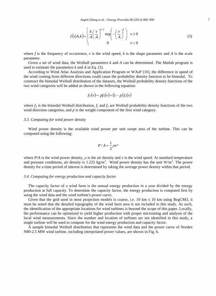
A sample bimodal Weibull distribution that represents the wind data and the power curve of Nordex

N80-2.5 MW wind turbine, including interpolated power values, are shown in Fig. 6.

8 Angeli Silang et al. / Energy Procedia 00 (2013) 000–000

Fig. 6. Sample Weibull distribution and Nordex N80-2.5 MW wind turbine power curve with wind speed as x-axis.

Power production can be computed by multiplying the frequency of the Weibull distribution to the

power production from the power curve at a particular wind speed. Energy production is the sum of the

production from each wind speed value multiplied by time. The equation for the energy production is the

following:

30

0.0v

vv tfPtPN

where P is power, N is the number of samples, t is the time period, Pv is the power produced for a given

wind speed v and fv is the frequency of v based on Weibull distribution.

As a default, Nordex N80-2.5MW will be used. This turbine has a rated power of 2.5 MW, a cut-in

wind speed of 4 m/s and cut-out wind speed of 25 m/s [11]. The wind speed has an interval of 1 m/s.

Linear interpolation was done to have an interval of 0.1 m/s.

The average wind speed and the turbulence intensity are some of the factors considered when

identifying the type of turbine. Nordex N80 is a class I turbine, which is built for a high turbulence site.

This turbine yields lower power output than a turbine of the same manufacturer and turbine model but of

lower class. Nordex N80 is chosen to yield conservative results since it is a class I turbine. The wind

turbine must be identified when applicable to ensure that the right type of turbine is used in the model.

Energy production may be improved when the appropriate turbine for the site is identified and the power

curve is provided.

The conversion model presented considers the seasonality of the wind and the possibility of observing

bimodal Weibull distribution of the wind speed. It also shows that power curves of wind turbines other

than the one provided could be used. The model is flexible that it can be used in different locations with

different requirements. This conversion model is applicable to offshore wind projection as much as it is

applicable to onshore.

4. Results and discussion

Projections of wind speed and wind direction from RegCM3 for a possible wind farm site in Pililla,

Rizal, Philippines are used. The projected wind data is divided into datasets of five years, which are 2013-

2017, 2018-2022, 2023-2027, 2028-2032 and 2033-2037. Each dataset has wind speed and wind direction

at heights of 10 m and 110.8 m. Wind data were interpolated to 80 m since this is the chosen hub height

for the turbine. The average value of the power law exponent α in Eq. (2) for the five datasets is 0.13.

Angeli Silang et al. / Energy Procedia 00 (2013) 000–000 9

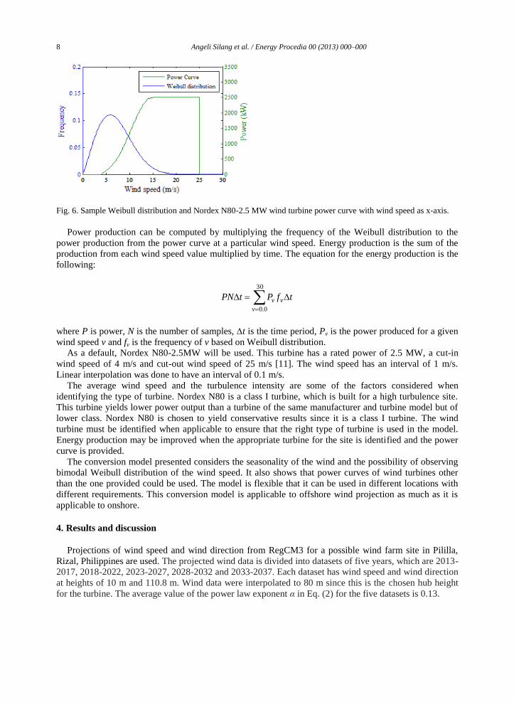
Both unimodal and bimodal Weibull distribution were used to compute for the average wind speed,

wind power density, and capacity factor. The bi-seasonal characteristic of wind in Pililla is not noticed in

the results since the Weibull distribution for the weaker and less frequent habagat overlaps with the

Weibull distribution for amihan providing a unimodal sum of the two functions. Fig. 7 illustrates the

unimodal and bimodal Weibull distribution functions. The histogram of the wind speed shows that there

is predominantly one mode for the distribution.

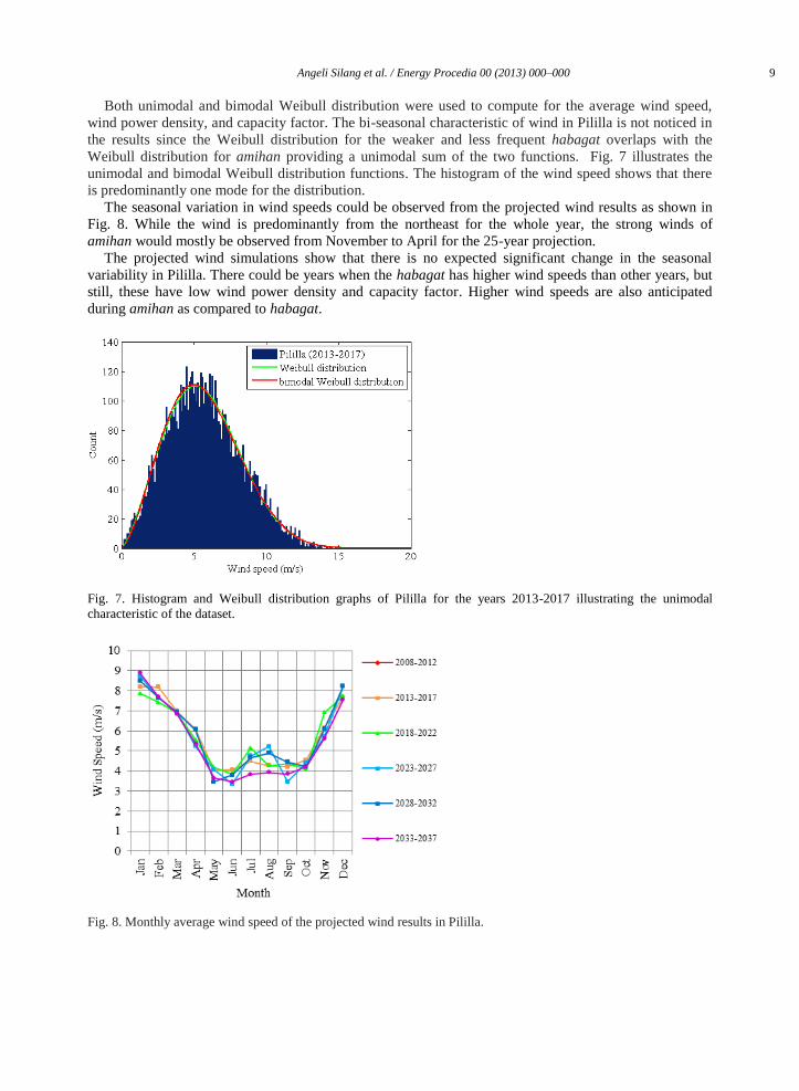
The seasonal variation in wind speeds could be observed from the projected wind results as shown in

Fig. 8. While the wind is predominantly from the northeast for the whole year, the strong winds of

amihan would mostly be observed from November to April for the 25-year projection.

The projected wind simulations show that there is no expected significant change in the seasonal

variability in Pililla. There could be years when the habagat has higher wind speeds than other years, but

still, these have low wind power density and capacity factor. Higher wind speeds are also anticipated

during amihan as compared to habagat.

Fig. 7. Histogram and Weibull distribution graphs of Pililla for the years 2013-2017 illustrating the unimodal

characteristic of the dataset.

Fig. 8. Monthly average wind speed of the projected wind results in Pililla.

10 Angeli Silang et al. / Energy Procedia 00 (2013) 000–000

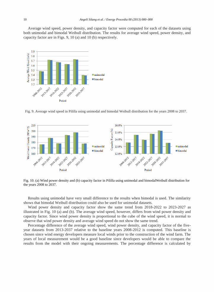
Average wind speed, power density, and capacity factor were computed for each of the datasets using

both unimodal and bimodal Weibull distribution. The results for average wind speed, power density, and

capacity factor are in Figs. 9, 10 (a) and 10 (b) respectively.

Fig. 9. Average wind speed in Pililla using unimodal and bimodal Weibull distribution for the years 2008 to 2037.

Fig. 10. (a) Wind power density and (b) capacity factor in Pililla using unimodal and bimodalWeibull distribution for

the years 2008 to 2037.

Results using unimodal have very small difference to the results when bimodal is used. The similarity

shows that bimodal Weibull distribution could also be used for unimodal datasets.

Wind power density and capacity factor show the same trend from 2018-2022 to 2023-2027 as

illustrated in Fig. 10 (a) and (b). The average wind speed, however, differs from wind power density and

capacity factor. Since wind power density is proportional to the cube of the wind speed, it is normal to

observe that wind power density and average wind speed do not show the same trend.

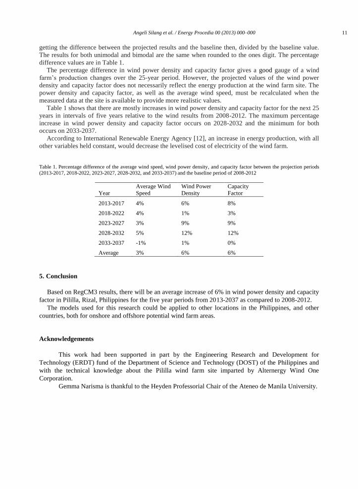
Percentage difference of the average wind speed, wind power density, and capacity factor of the five-

year datasets from 2013-2037 relative to the baseline years 2008-2012 is computed. This baseline is

chosen since wind energy developers measure local winds prior to the construction of the wind farm. The

years of local measurement would be a good baseline since developers would be able to compare the

results from the model with their ongoing measurements. The percentage difference is calculated by

Angeli Silang et al. / Energy Procedia 00 (2013) 000–000 11

getting the difference between the projected results and the baseline then, divided by the baseline value.

The results for both unimodal and bimodal are the same when rounded to the ones digit. The percentage

difference values are in Table 1.

The percentage difference in wind power density and capacity factor gives a good gauge of a wind

farm’s production changes over the 25-year period. However, the projected values of the wind power

density and capacity factor does not necessarily reflect the energy production at the wind farm site. The

power density and capacity factor, as well as the average wind speed, must be recalculated when the

measured data at the site is available to provide more realistic values.

Table 1 shows that there are mostly increases in wind power density and capacity factor for the next 25

years in intervals of five years relative to the wind results from 2008-2012. The maximum percentage

increase in wind power density and capacity factor occurs on 2028-2032 and the minimum for both

occurs on 2033-2037.

According to International Renewable Energy Agency [12], an increase in energy production, with all

other variables held constant, would decrease the levelised cost of electricity of the wind farm.

Table 1. Percentage difference of the average wind speed, wind power density, and capacity factor between the projection periods

(2013-2017, 2018-2022, 2023-2027, 2028-2032, and 2033-2037) and the baseline period of 2008-2012

Year

Average Wind

Speed

Wind Power

Density

Capacity

Factor

2013-2017 4% 6% 8%

2018-2022 4% 1% 3%

2023-2027 3% 9% 9%

2028-2032 5% 12% 12%

2033-2037 -1% 1% 0%

Average 3% 6% 6%

5. Conclusion

Based on RegCM3 results, there will be an average increase of 6% in wind power density and capacity

factor in Pililla, Rizal, Philippines for the five year periods from 2013-2037 as compared to 2008-2012.

The models used for this research could be applied to other locations in the Philippines, and other

countries, both for onshore and offshore potential wind farm areas.

Acknowledgements

This work had been supported in part by the Engineering Research and Development for

Technology (ERDT) fund of the Department of Science and Technology (DOST) of the Philippines and

with the technical knowledge about the Pililla wind farm site imparted by Alternergy Wind One

Corporation.

Gemma Narisma is thankful to the Heyden Professorial Chair of the Ateneo de Manila University.

12 Angeli Silang et al. / Energy Procedia 00 (2013) 000–000

References

[1] Ren D. Effects of global warming on wind energy availability. Journal of Renewable and Sustainable Energy 2 2010;

052301.

[2] Greene JS, Chatelain M, Morrissey M, Stadler S. Projected future wind speed and wind power density trends over the

Western US High Plains. Atmospheric and Climate Sciences 2012; 2:32-40.

[3] Elliot DL. Philippines wind energy resource atlas development. Colorado: National Renewable Energy Laboratory;

November 2000.

[4] Elguindi N, Bi X, Giorgi F; RegCM version 3.1 user guide. Italy: Abdus Salam International Centre for Theoretical Physics;

2007.

[5] Villafuerte II M, Narisma G. The potential impact of global warming on southwest monsoon rainfall in the Philippines.

Conference Proceeding: Asia-Oceania Geosciences Society 8th Annual Meeting and Geosciences World Community Exhibition;

Taipei; 8-12 August 2011.

[6] Villafuerte II M. The Philippines’ southwest monsoon season in the next thirty years: A regional climate projection.

Philippines: Ateneo de Manila University; 2010, p. 69.

[7] Gipe P. Wind Power: Renewable Energy for Home, Farm, and Business. USA: Chelsea Green Publishing Company; March

2004, pp. 40-41.

[8] Ray ML, Rogers AL, McGowan JG. Analysis of wind shear models and trends in different terrains. Conference Proceeding:

American Wind Energy Association Windpower; Anaheim; 22-25 May 2006.

[9] Manwell J, McGowan J, Rogers A. Wind Energy Explained: Theory, Design and Application. 2nd ed. Great Britain: John

Wiley & Sons, Inc.; 2009, pp. 46-47.

[10] WasP 10 on-line help file. Wind Atlas Analysis and Application Program. Retrieved from

http://www.wasp.dk/Support/Literature.aspx

[11] Nordex N80/N90 brochure. Retrieved from http://vetropark.org/d/59743/d/nordex_n80-n90_gb.pdf

[12] Renewable Power Generation Costs in 2012: An Overview. International Renewable Energy Agency; 2013. Retrieved from

http://www.irena.org/Publications