2008/62 ■

Average power contracts can mitigate carbon leakage

Giorgia Oggioni and Yves Smeers

CORE Voie du Roman Pays 34 B-1348 Louvain-la-Neuve, Belgium. Tel (32 10) 47 43 04 Fax (32 10) 47 43 01 E-mail: corestat-library@uclouvain.be http://www.uclouvain.be/en-44508.html

CORE DISCUSSION PAPER 2008/62

Average power contracts can mitigate carbon leakage

Giorgia OGGIONI 1 and Yves SMEERS2

November 2008

Abstract

The progressive relocation of part of the Energy Intensive Industries (EIIs) out of Europe is one of the possible consequences of the combination of emission charges and higher electricity prices entailed by the EU-Emission Trading Scheme (EU-ETS). In order to mitigate this effect, EIIs have asked for special power contracts whereby they would be supplied from dedicated power capacities at average (capacity, fuel, transmission and emission allowance) costs. We model this situation on a prototype power system calibrated on four countries of Central Western Europe. In order to capture the main feature of EIIs' demand, we separate the consumer market in two segments: EIIs and the rest. EIIs buy electricity at average cost price while the rest pays marginal cost. We consider two different types of EIIs' contractual arrangements: a single region wide and zonal average cost prices. We also analyze the cases where generators only rely on existing capacities or can invest in new ones. We find that these average cost contracts can indeed partially mitigate the incentive to relocate activities but with quite diverse regional impacts depending on different national power policies. Models are formulated as a non-monotone complementarity problems with endogenous energy, transmission and allowance prices and are implemented in GAMS. Keywords: average cost based contracts, carbon leakage, complementarity conditions, EU-ETS.

1 Università degli Studi di Bergamo, Italy and CORE, Université catholique de Louvain, Belgium. E-mail: giorgia.oggioni@unibg.it 2 Tractebel Professor of Energy Economics, INMA and CORE, Université catholique de Louvain, Belgium. E-mail: yves.smeers@uclouvain.be. This author is also member of ECORE, the newly created association between CORE and ECARES. This work has been financially supported by the Italian project PRIN 2006, Generalized monotonicity: models and applications whose national responsible is Prof. Elisabetta Allevi and by the Chair Lhoist Berghmans in Environmental Economics and Management. The authors gratefully acknowledge Thierry Bréchet, Andreas Ehrenmann and Chefi Triki for their in depth comments and helpful advices.

This paper presents research results of the Belgian Program on Interuniversity Poles of Attraction initiated by the Belgian State, Prime Minister's Office, Science Policy Programming. The scientific responsibility is assumed by the authors.

1 Introduction

Climate change is a global issue but the mitigation of its development and extent is stillseen as a regional matter that can be handled by a diversity of means decided at locallevel (see the argument of Pizer [15]). The EU, with its Emission Trading Scheme (EU-ETS or more briefly ETS), has taken the lead in this endeavour, possibly at the risk ofendangering the competitiveness of part of its industry. The ETS is a cap and trade systemthat introduces a price for each unit of GHG emitted by the combustion installations coveredby the scheme. This creates costs, both direct and indirect, for the companies operating theseinstallations. The direct costs (hereafter carbon cost) accrue from the obligation to eitherbuy allowances or reduce emissions. The indirect cost (hereafter electricity cost) is due tothe higher price of electricity that results from the pass-through of allowance (opportunity)costs in the price of electricity. Both add up and modify the operations costs of the affectedEnergy Intensive Industries (hereafter EIIs). This impact depends on the industrial sectorand may be important for some of the EIIs covered by the ETS.

EIIs have argued that the ETS endangers their competitive positions with respect tocompanies of the same sectors located in environmentally less restrictive countries. Theyalso explain that they will relocate some or all of their activities in these countries in orderto protect their competitiveness. This would reduce emissions in Europe but increase themoutside of the EU. This would result in no environmental benefit but could cost Europesignificant economic and job losses. The expression “carbon-leakage” refers to this relocationof economic activity and emissions.

The impact of the ETS on industrial activity depends on several factors, among them(i) the industry’s ability to pass the extra carbon cost onto the final consumer, (ii) theopenness of international trade (iii) the energy intensity of the sector and its capability toabate carbon, (iv) the allowance allocation method and (v) the product specialization. Thesedifferent factors combine to determine whether the sector is largely exposed to internationalcompetition or protected. Service oriented economies will obviously suffer less from the ETSthan those that heavily rely on highly emitting technologies. Delgado [3] elaborates on thecomparatively large part of energy intensive goods in EU export, a phenomenon that isobviously worrying for a region that intends to take the lead in abatement measures.

Opinions diverge on the importance of carbon leakage. The “Climate Strategy group”(Hourcade et al. [9]) plays down the danger for Europe. The authors explain that iron andsteel, aluminium, cement and lime are the only sectors that can be affected by the ETS;they study the UK where these sectors altogether represent only 1% of GNP and concludethat the problem is minor and particular solutions can probably be found. The proposal forborder adjustment defended by the French government during its presidency of the EU sug-gests a less optimistic view. The idea of the border adjustment is to counter carbon leakageby supporting exports by EU industries affected by carbon leakage and taxing those goodsimported from countries with a more lenient environmental system. This proposal clearly ac-knowledges a problem of competitiveness due to carbon leakage. The European Commissiondoes not discard this possibility either. Its “Impact Assessment”1 admits “until a compre-hensive international agreement would be reached, carbon leakage could occur underminingthe overall environmental objective of EU climate and energy policies”. The need to protect

1See Impact Assessment, document accompanying the Package of Implementation measures for the EU’sobjectives on climate change and renewable energy for 2020, Brussels, January 23, 2008. Available at http ://ec.europa.eu/environment/climat/climate action.htm.

2

the competitive position of the EU industry has accordingly been taken into account in thedesign of the proposal of the ETS Directive for the period 2013-2020. Specifically, point 8of Article 10a of the Directive proposal states that “in 2013 and in each subsequent year upto 2020, installations in sectors, which are exposed to a significant risk of carbon leakageshall be allocated allowances free of charge up to 100 percent of the quantity determinedin accordance with paragraphs 2 to 6”2. This measure will be adopted in case of failure ofinternational environmental negotiation whose conclusions is foreseen by the year 2011.

Not unexpectedly, representative of the EIIs are most vocal about the impact of the ETSon their costs. Their position should not necessarily be seen as pure lobbying. These sectorsgenerally consist of multinational companies that operate worldwide and hence could relocatepart of their production without suffering dramatic economic losses themselves. They wouldincur transient costs but no long-term damage; their message can plausibly be interpreted asadvising that European economies and populations, not the firms themselves, would loose agreat deal in the long run.

EIIs have proposed two remedies. One is to introduce sectorial agreements whereby firmsof a given sector would agree to reduce emissions. This has so far not materialized. EIIs alsoproposed another measure that today has seen two example of implementation. EIIs haveindeed argued about carbon leakage to demand special electricity contracts to counter theimpact of the ETS on electricity price. The objective of these contracts is to isolate EIIsfrom the joint effect of passing the ETS emission allowance (opportunity) costs in electricityprices in carbon dominated systems, and aligning European electricity prices on these carboninclusive prices because of the progressive integration of the electricity market. Specificallythe Finnish pulp and paper industry has succeeded to obtain such a contract with the fifthnuclear power plant that the Franco-German consortium formed by Areva and Siemens isbuilding at Olkiluoto on the western coast of Finland3. This principle also underlines inthe formation of the Exeltium consortium in France where a number of electro-intensiveindustries4 have managed to conclude long term contracts with EdF5. In both cases, longterm competitiveness and price stability are the arguments invoked to justify these contracts.

This paper is about these contracts: we introduce these special contracts in a prototypemodel of the European power sector and provide a first assessment of their impact on in-vestments in the power sector and their capability to mitigate the impact of the ETS onEIIs.

An in-depth study of the true impact of special contracts such as those implied in Exeltiumis probably impossible today. A major difficulty is the lack of adequate information on thereaction of the EIIs to changes of carbon and electricity prices: we know that the ETS affectsthese sectors but we are currently unable (from outside the industry) to quantify the impactof carbon and electricity prices on their activities. But the situation is temporary; piecesof information are progressively collected and knowledge is progressively accumulating. We

2Source:http://ec.europa.eu/environment/climat/emission/pdf/ets revision proposal.pdf.3Sources: http://virtual.finland.fi/netcomm/news/showarticle.asp?intNWSAID=28308 and

http://virtual.finland.fi/netcomm/news/showarticle.asp?intNWSAID=25870.4These are: Air Liquide, Alacan, Arcelor Mittal, Arkema, Rhodia, Solvay and UPM-Kymmene.5After negotiations lasted almost three years, EdF and Exeltium have finalized their partnership agreement

following the initiative launched by the government in 2005. With this agreement, industrial consumers whoare Exeltium shareholders are securing part of their electricity supply over the long term. EdF is optimizingthe use of its production facilities by supplying around 13 TWh per year, over a total of 24 years (seeEdF press release at http://www.edf.fr/the-edf-group/press/press-releases/noeud-communiques-et-dossier-de-presse/edf-group-and-exeltium-finalise-partnership-agreement-600379.html).

3

already mentioned the analysis conducted by the Climate Strategy group on the basis of theUK. It would be interesting to know whether similar industrial structures apply throughoutthe EU or will eventually apply as industrial activities move to emerging economies (McK-insey&Company [10]). Short-term Armington elasticity, such found in (Hourcade et al. [9]),cannot provide the basis for long- term substitution analysis but process models such as thosepresented by Hidalgo et al. [8] and Szabo et al. [16] can. Also IEA is conducting an in depthquestion of this problem. An other difficulty, probably much less pressing, is the insufficientdevelopment of our European power models. The sector is central to the problem of carbonleakage and the EIIs, but its representation cannot be limited to the sole generation side. Thespatial arrangement and hence the representation of the grid are central for responding to theEIIs’ question for special contracts. Even though power models that involve a representationof the grid are not numerous, they are progressively emerging. We use a prototype modelhere but mention current activities such as Duthaler et al. [6], Perekhodtsev [14] and Zhouand Bialek [17].

This paper takes stock of this emerging activity and provides a prototype study of theimpact of special contracts such as those implied by Exeltium, possibly combined with freeallowances as foreseen by the Commission’s proposals. The paper is organised as follows:Section 2 describes the principle of the special contracts demanded by EIIs. Section 3 presentsour methodology and Section 4 is devoted to the models and input data. Sections 5, 6 and7 explain the main results and Section 8 concludes. The model used is described in Oggioniand Smeers [12],[13].

2 Cost Based Electricity Contracts

Investments in both EIIs and the power sectors are capital intensive and long term. Asdiscussed in the introduction, schemes such as the ETS affect these investments in at leasttwo ways. By imposing the covered EIIs an obligation either to abate or surrender an emissionallowance per ton of emitted CO2 equivalent, the ETS directly increases the production costof the firms in these industries. By imposing a similar obligation to the power sector, the ETSalso entails an increase of the price of electricity and hence further raises the production costof the EIIs. These two phenomena come on top of a general evolution that sees a progressivemovement of large energy consuming industries away from developed to emerging economies(McKinsey&Company [10]). New investments of EIIs in Europe, which may already bequestioned in the current economic conditions are then becoming more at risk as a result ofthis double cost effect. Recall that this risk is incurred without any environmental benefit in acarbon leakage context: emissions are not reduced but simply displaced from Europe to otherplaces of the world. Emissions will even probably increase to the extent that the displacedinstallations connect to less carbon efficient power systems. This relocation of industrialconsumption introduces a demand risk that adds to the already uncertain environment thatsurrounds investments in the power sector.

Contracts that guarantee the delivery of electricity on the long run (e.g. 15 years) ata controllable overall cost, possibly backed by dedicated capacities, can mitigate that riskand reduce the cost, benefiting both EIIs and the power sector. The principle of thesecontracts is straightforward even if their implementation may be complex: an energy intensiveconsumer procures electricity forward over a long period by essentially paying its full cost(investment and operations) independently of the vagaries of the prices on power exchanges.

4

This contact is normally for high load electricity, corresponding to a base activity of theelectricity consuming EII firms. It is thus associated to a base load unit, which, becauseof its high capital cost is more risky to invest in without a long term guarantee of deliveryeven if it is cheaper to operate. The electricity price contains a fixed part corresponding tothe investment cost. It may contain a variable fuel part, which is in any case a world price(coal or nuclear fuel). If fossil fuel based, the electricity price would also contain a CO2

contribution. The principle of the cost based contract is that this CO2 contribution wouldbe paid at average cost and not according to a marginal cost principle that EIIs object to.EIIs argue that marginal cost pricing increases electricity prices and they advocate a returnto average cost pricing. As in the Finnish and the Exeltium consortium cases, EIIs ask forthese cost based electricity contracts, possibly backed by dedicated facilities.

3 Methodology

3.1 Model Description

The problem of the possible impact of the ETS on EII sectors is long term. We accordinglycast average cost power contracts in a model that can accommodate, at least partially in thispaper, investments in new capacities. In order to do so, we construct a power model (seeOggioni and Smeers [12], [13]) where demand is decomposed into two segments; one segmentconsists of the firms of the covered EII sectors (EIIs hereafter), the other segment gathers therest of the demand (N-EIIs hereafter). The power sector is represented by a process modelwhere the different generation plants are explicitly described on a technological basis 6. Thesemodels are well mastered both in the literature and in practice and the representation adoptedin this paper is standard. The demand sectors are described differently. We classically modelthe N-EIIs’ sector by a demand function. We would also ideally adopt a process modelfor describing the EIIs, but even though these exist for the cement and steel sectors (seeDemailly and Quirion [4], Hidalgo et al. [8] and Szabo et al. [16]), they are far from standardtoday. One can also note that while GHG studies extensively rely on power sector models,they generally adopt a much simpler description of the consuming sectors. We follow suitand simplify the description of the EIIs into a linear demand function that that we calibrateon the basis of Newbery [11]. This modelling of the EII sectors implies that we interpret areduction of their demand as a relocation of activities that measures the carbon leakage effect.This is admittedly a rough representation of the reaction of these industries as it does notdifferentiate between activity relocation and energy efficiency improvements. Still it sufficesto qualitatively capture the impact of the ETS on EIIs. We shall show that it also allowsone to represent both the carbon and the electricity costs and hence permits differentiatingbetween different policies of free permits allocations to the energy consuming sectors.

Throughout the paper we make the blanket assumption that all agents are price takersor alternatively that large energy consumers can impose average cost pricing on generators(or that they can build their own units and hence procure electricity at average cost). Wejustify the assumption as follows. While it is apparently easy to find evidence of the exerciseof market power by generators, the literature shows that it is equally easy to criticize thisevidence. Moreover there is no well admitted paradigm for modeling the exercise of marketpower by generators (Cournot is technically simple and supply functions difficult; but none ofthem is substantiated by convincing empirical evidence). Introducing market power is thus

6Different type of generation units with their technological characteristics.

5

a somewhat arbitrary exercise outside studies that explicitly aim at measuring its exercise.Note that this blanket assumption does no imply that all models presented here are of theperfect competition type as average cost pricing deviates from the long run marginal costpricing which would be the rule in perfect competition. Last we mention that our modelsalways account for the emissions of the power sector, and in some version (see infra) alsofor the emissions of the EIIs. Emissions are capped, which implies that the price of CO2 isendogenous.

Transmission is represented according to a flowgate model which is the approach currentlydiscussed for CWE by transmission system operators. This network model is well known inthe literature7. The representation includes a node, the so–called hub node, where electricityasks and bids converge and clear. The hub can be considered as a virtual market that setsthe electricity price. In this system, generators send the electricity they produce to the hubwhere energy is withdrawn and delivered to consumers located in the different nodes. Powertrade must respect the capacity limit of the lines composing the grid. A Power Transfer Dis-tribution Factor PTDF matrix determines both the directions and the proportions of powerflowing through network lines as a function of nodal injections and withdrawals. Constraintsimpose that the sum over all nodes of the proportion of the net power flow injected intoand withdrawn from all nodes and passing through a network line to reach the hub mustbe lower than the capacity of the line used to transfer electricity. This limits the set ofpossible injections and withdrawals. Congestion arises when at least one of the grid lines isoverloaded. National Transmission System Operators (TSO hereafter) are in charge of reliev-ing the network congestion and their operating costs are paid by final electricity consumers.Congestion costs are added to the electricity price set at the hub and differ with generatorsand consumers’ locations in the network. We work with a zonal representation of the gridthat therefore implies a zonal pricing system.

3.2 Analysis Structure

We consider three views of the problem of increasing technical complexity and discuss resultsin Sections 5, 6 and 7 respectively. The first two views (hereafter referred to as “IFC”(Indirect ETS costs with Fixed Capacity) and “II” (Indirect ETS costs with Investments)respectively) concentrate on the pass-through of allowance prices in electricity prices (theelectricity cost). The first version of the problems (IFC) assumes fixed generating capacities,the second one (II) allows for possible investments. The latter cases (II) are obviously morerealistic, but we also retain the simpler fixed capacity (IFC) cases because they allow for afirst, simpler, presentation of the phenomena. Both views of the problem are constructed byassuming an emission cap for the sole power sector, without any trade of allowances withthe EIIs. The third view of the problem, hereafter referred to as “DII” (Direct and IndirectETS costs), additionally deals with the carbon effect, that is the net effect for EIIs of tradingallowances on the market, taking into account their emissions and the allowances that theyreceive free. We cast both the carbon and electricity costs in the electricity demand functionof EIIs. The industrial electricity consumption is then affected by two factors: the electricityprice, which embeds the “electricity cost” and a carbon component which is the “carbon cost”and reflects the EIIs’ position on the emission market. In this latter view of the problem(DII) we also modify the emission constraint in order to account for the emissions derivingfrom the industrial production activities.

7See the section on flowgate on the HEPG website.

6

These different view of the carbon leakage problem, considering first the increase of elec-tricity prices (IFC and II models) and then the combination of both this increase and thetrading of allowances by EIIs (DII) is also quite in line with practice as representatives ofthe EIIs mainly complained about high electricity prices during the first compliance periodof the ETS.

Each of these three views of the carbon leakage problem in turn gives rise to four modelsthat we respectively note by NETS R, ETS R, ETS SAC and ETS ZAC. The first model(NETS R) adopts the perfect competition paradigm in the sense that the two demand seg-ments pay an identical electricity price that is equal to the marginal production cost of theunit that is highest in the merit order. It also supposes that there is no ETS. The secondmodel (ETS R) works under the same perfect competition scenario, but assumes that the ETSis in force. We introduce these cases both for reference and calibration purposes. The perfectcompetition paradigm under the ETS indeed includes a full pass-through of the marginal(opportunity) cost of allowances in the price of electricity, independently of the procurementof these allowances by power companies. This is the situation that EIIs complain aboutwhen they refer to the windfall profits of the power companies that pass in the electricityprice the allowances that they partially received free. In order to introduce the cost basedelectricity contracts, we modify this reference model by splitting the capacity in two partsendogenously dedicated to each market segment. Generators then adapt their generation mixto the pricing scheme in each market segment. N-EIIs face the marginal cost price of theirdedicated capacities that adapt to their time varying demand. EIIs benefit from the averagecost contracts suited to their high load demand. We then consider two different average costcontracts respectively identified by ETS SAC and ETS ZAC that reflect prevailing and pos-sibly forthcoming conditions in the European electricity market. The first pricing scheme isregional and referred to as ETS SAC. It assumes that the transmission system has developedto a stage that EIIs can and do procure electricity on a regional basis. The region in thiscase is Central West Europe, hereafter CWE (see ECN [7]); it consists of Belgium, France,Germany and the Netherlands. All EII firms in the the region pay the same average cost thatincludes the full generation cost (capacity, fixed and variable operating, fuel and CO2 costs)of the dedicated capacities and the transmission cost (congestion charges) from generation toEII consumers. The latter is computed according to a flowgate model mentioned above. Thecase law of European competition authorities considers that this regional market is not es-tablished yet. The second pricing scheme takes stock of this jurisprudence and supposes thatEII firms procure electricity at average cost on a local, here zonal basis, hereafter referred toas ETS ZAC. This average cost then boils down to the full average generation cost (capacity,fixed and variable operating, fuel and CO2 costs) of the dedicated capacities of the zone,without any transmission component. Both ETS SAC and ETS ZAC models are inspired bythe approach followed by French EIIs when constituting the Exeltium consortium in orderto buy electricity from generators at a French market-wide full cost based price. The twoaverage cost pricing schemes, ETS SAC and ETS ZAC, considered here only differ by theregional scope of the consortium and the implication of the transmission component on theaverage cost price. Finally, we consider the so–called “EIINA” and “EIIA” scenarios whichrespectively indicate the cases where EIIs do not receive and receive free allowance when theyparticipate to the emission market.

N-EIIs and EIIs’ fuel costs, capacity costs and reference demands are identical throughoutthe three views. This allows us to examine the evolution of results under different organiza-tional scenarios without data playing an impact on the results. This step by step methodology

7

also allows us to analyze the EIIs’ problem under progressively more complex aspects. Notethat the structure of the average cost price models is such that generators are constrained toconclude average cost based contracts with EII companies which in turn can exercise monop-sony power since have access to dedicated power. An interesting question is whether powercompanies effectively gain from the application of these long term contracts. This is reportedin the welfare analysis. We summarizes the overall structure of the analysis and the differentmodels and their nomenclature in Table 1.

ModelsAnalysis Steps Leakage Mitigation ScenariosIFC NETS R ETS R ETS SAC ETS ZACII NETS R ETS R ETS SAC ETS ZACDII EIINA NETS R EIINA ETS R EIINA ETS SAC EIINA ETS ZAC

EIIA NETS R EIIA ETS R EIIA ETS SAC EIIA ETS ZAC

Table 1: Analysis Steps and Scenarios

4 Model Setting

The analysis is applied to a stylized representation of the Central Western European (CWE)power market depicted in Figure 1. Data of this model are available on the Energy ResearchCenter of the Netherlands (ECN [7]) website. We also calibrate the rest of the model for theyear 2005 which saw the inception of the ETS and is also the first year for which emissionsare recognized to be independently and consistently verified.

The power market depicted in Figure 1 comprises fifteen nodes distributed over fourcountries: Germany, France, Belgium and the Netherlands. Electricity production and con-sumption activities are aggregated in seven nodes: two in Belgium (Merchtem and Gramme),three in the Netherlands (Krimpen, Maastricht and Zwolle), one in Germany (“D”) and,finally, one in France (“F”). The remaining German and French nodes are passive and areonly used to transfer electricity. Nodes are connected by 28 flowgates with limited capacity.There are 10 cross-border flowgates: two connect Germany and the Netherlands and threelink the Netherlands and Belgium; there are three lines between Belgium and France andtwo between France to Germany. The model of the grid follows the standard DC load flowapproximation: flowgates are characterized by limited transfer capacities, which constrainpower flows, and by Power Transmission Distribution Factors (PTDF ) that distribute injec-tion and withdrawals of electricity along the lines. These data (see ECN [7]) are reported inFigure 1. The big German node is the hub node where all power asks and bids converge anddefine the system electricity price.

As foreseen by the FlowBased Market Coupling project of the CWE’s electricity systems,the clearing of this market results from an interaction between the PXs and the TSOs ofthe region that can be assimilated to the solution of a consumer and producer surplus max-imization in CWE subject to transmission constraints. The system currently operates onthree countries only (the above minus Germany) and still uses a representation of the gridby transmission capacities. It should include Germany and move to the flow based represen-tation of the grid soon. We anticipate this evolution and directly adopt the flow based, orflowgate representation of the grid. This system introduces a market of transmission rightsthat agents pay for to the Transmission System Operators.

8

Figure 1: Central Western European market and network line capacities

We assume eight European power companies8 plus a fringe which assembles the remainingsmall generators. These companies supply this market by running eight different technologies:hydro, renewable, nuclear, lignite, coal, CCGT, old gas and oil based plants. These units areranked in merit order that is endogenously determined as a function of the (exogenous) fuelprices and the (endogenous) transmission constraints. This assumption implies a staircaserepresentation of the supply curves whose shape is directly influenced by the marginal costsof the different technologies. Plant capacities’ values are taken from the public 2005 reportsof the power companies included in the models.

Depending on the view of the problem (see Section 3), electricity is produced either byexisting or new power plants. In order to simplify both the database and the interpretationof the results, we assume that old and new capacities have identical variable and fixed costs.The models obviously allows one to change this assumption and apply different efficiencyrates to new plants. Doing so in this prototype study would however cloud the results thatwould then be influenced by both fundamental economic phenomena and sometimes arbitrarydata differentiations.

Generators supply both EIIs and N-EIIs. For reasons explained in Section 3, it is currentlyquite difficult to resort to sectorial models of the EIIs sectors, whether process or econometricmodels. We use linear demand functions to describe these two consumer groups. We constructthem by setting a reference power price of 40 e/MWh and reference elasticity values of -0.1and -1 respectively for N-EIIs and EIIs. As already said, the -1 value is taken from Newbery[11]. This elasticity’s assumption may appear too high, but our goal is to get insight intothe way cost based contracts mitigate the EIIs’ difficulties. We are not in a position in thispaper to come up with a precise quantification of these effects9.

The period analyzed is one year composed of 8760 hours subdivided into two sub-periods:the so–called summer (5136 hours) and winter (3624 hours). We are thus effectively workingwith the base-load demand of each consumer group in winter and in summer. We differentiatethis based load demand by node. We suppose, as is the case in CWE, that N-EIIs have a

8EdF, Electrabel, E.ON Energie AG, ENBW Energieversorgung Baden-Wurttemberg, Essent Energie Pro-ductie BV, Nuon, RWE Energie AG and Vattenfall Europe.

9Nevertheless, we also tested the case where the industrial demand elasticity equals -0.8 to verify therobustness of our results.

9

higher power demand in winter than in summer. EIIs’ power demand is constant over theyear.

After transmission rights and electricity, emission allowances constitute the third com-modity exchanged on this market. The carbon market is simply modelled by an emissionconstraint where the total cap is computed on the basis of the data available from the Commu-nity Independent Transaction Log ([1]). We used the report by Davis and URS Corporation[2] as a reference for the emission factors of the different generation technologies. We ex-plain the computation of EIIs’ emission factors in Appendix G. We assume full auctioning ofallowances to generators and a benchmarking method for allocating free allowances to EIIs.

We follow the structure of analysis introduced in Section 3 and accordingly first presentthe results of the models with fixed generation capacity. We later allow generators to investin new power plants and finally consider the scenarios where EIIs are inserted in the ETS. Inorder to simplify the notation we do not refer to the section identifier (IFC, II, DII. See Table1) when discussing results obtained under the assumptions of the section. Various appendicesprovide additional information. Oggioni and Smeers [12], [13] give the technical details of themodel.

5 Indirect Electricity Cost with Fixed Capacity Scenarios (IFC)

Table 2 reports the global impact of the different policy scenarios on electricity demand, thatwe analyze in more details in this section.

TWh N-EIIs EIIs TotalIFC NETS R 649 598 1,248IFC ETS R 646 531 1,177IFC ETS SAC 634 555 1,189IFC ETS NAC 623 565 1,188

Table 2: EIIs’ hourly demand without and with the EU-ETS

As announced, we drop the section’ s identifier (here “IFC”) when referring to scenariosconducted with fixed capacity.

5.1 Reference Case with (IFC ETS R) and without (IFC NETS R) ETS

The inception of the ETS emission trading globally decrease EIIs’ electricity consumptionfrom 598 TWh (NETS R) to 531 TWh (ETS R). N-EIIs’ reduction is from 649 TWh to 646TWh. The pricing effects leading to that reduction of demand are analyzed in Appendix B.1.The fall of EIIs’ demand is significant but driven by our assumption of a long-term EIIs’ priceelasticity of -1 at the reference demand point of 40 e/MWh. It illustrates the EIIs’ threat of along-term relocation of some of their facilities outside of Europe and the carbon leakage thatit implies. It also highlights the importance for Europeans of properly and rapidly assessingthe effective reaction of the EIIs to the changing electricity price implied by the ETS.

The decreased electricity demand and the utilization of less polluting technologies alsoimply an emission reduction. There is a cut of CO2 emissions from 464 Mio Ton before theinception of the ETS (NETS R) to 397 Mio Ton (ETS R) which is the cap imposed on thepower sector in this stage of analysis. The allowance price amounts to 24.44 e/ton.

10

5.2 Regional (IFC ETS SAC) and Zonal (IFC ETS ZAC) price

Average cost pricing policies partially relieve EIIs’ burden while maintaining the global emis-sion target. On the positive side, both the regional (ETS SAC) and the zonal (ETS ZAC)prices increase EIIs’ electricity consumptions compared to the reference marginal cost prices(ETS R). The negative side is that not all EIIs benefit from the application of these pricingschemes and the final results depend on national energy policies. The increase of demanddoes not go as far as recovering the activity levels observed before the inception of the ETS.

The regional price (ETS SAC) increases EIIs’ consumption from 531 TWh to 555 TWh.EIIs enjoy lower electricity prices in Germany, the Netherlands and in the Belgian locationMerchtem, which increase their activities. In contrast the single price policy increases EIIspower costs in France and the other Belgian node Gramme with a consequent decrease of theirelectricity consumption. The price increase is particularly high in France (+69%) where EIIs’electricity consumption falls from 218 TWh to 170 TWh. In Gramme, the decrease is just of1% (from 17,2 TWh to 17 TWh). These EIIs’ demand decreases are globally compensatedby increases in other nodes, leading to the final aforementioned 5% augment of the EIIs’demand (Table 2).

The zonal price (ETS ZAC) also has a global positive effect on EIIs. It increases their elec-tricity consumption from 531 TWh to 565 TWh compared to marginal cost pricing (ETS R)and with an increase from 555 TWh to 565 TWh does slightly better than the single price(ETS SAC). But here again, this global positive effect results from quite different local im-pacts on EIIs. Nuclear capacity in France and in the Belgian node Gramme, combined withzonal pricing system drastically mitigates the EIIs’ electricity costs in these locations. EIIsare supplied by local power plants in this regime and do not have to share cheap and cleanelectricity with foreign EIIs’ plants as in the single price (ETS SAC) scenario.

The situation of EIIs is more critical in countries where electricity is mostly produced byfossil technologies as in the Netherlands and the Belgian node Merchtem. Industries effec-tively suffer from the zonal price policy. In Germany, the industrial electricity consumptiondecreases from 270 TWh to 236 TWh with respect to the single price (ETS SAC), but re-mains 7% higher than in the marginal cost pricing case (ETS R) where the consumption levelis 220 TWh.

This global improvement of the EIIs’ situation resulting from an economically inefficientpolicy (average cost pricing) is to be paid somewhere. One indeed observes that the singleand the zonal prices respectively decrease N-EIIs’ electricity consumption from 646 TWh to634 TWn (ETS SAC) and from 646 TWh to 623 TWh (ETS ZAC) compared to marignalcost pricing policy (ETS R).

5.3 Welfare Analysis

The welfare analysis of Table 3 gives an alternative view of these results. The lines “EIIs”,“N-EIIs” and “Consumers” are self-explanatory. The lines “Generators” and “Allowances”respectively report the generators’ profits and the allowance values obtained by multiplyingthe market cap of 397 Mio ton p.a. by the allowance prices of the different scenarios (anallowance comes at 28.48 e/ton and at 28.21 e/ton in the regional (ETS SAC) and zonal(ETS ZAC) pricing systems. The generators’ profits are computed assuming fully grandfa-thered allowances and hence are higher than before the inception of the ETS (NETS R).Generators’ profits decrease when allowances are totally or partially auctioned. In case offull auctioning the generators’ profits are obtained by subtracting the allowance value from

11

the profit reported at the “Generators” line. Note that this profit representation allows us toevaluate the impacts of different proportions of free allocation on generators’ profits. Finally,Table 3 lists the TSO’ merchandising profits in the different cases. These profits accrue fromthe application of the flowgate model to manage the congestion of the transmission system.

Except for the single price scenario, (ETS SAC), EIIs’ surpluses evolve in parallel withelectricity consumption. The decrease of EIIs’ surplus in the regional price policy, notwith-standing the global consumption increase, results from the significant drop (-47%) of theFrench EIIs’ surplus which is not compensated by increases in other nodes. Recall thatFrench EIIs reduce their power demand by 22% in this regional price regime.

Billion e IFC NETS R IFC ETS R IFC ETS SAC IFC ETS ZACEIIs 15.53 12.08 11.64 13.49N-EIIs 130.87 129.35 124.65 120.20Consumers 146.40 141.43 136.29 133.69

Generators 25.22 29.25 32.94 36.78Allowances 9.70 11.32 11.21

TSO 0.65 0.90 1.26 0.10

Welfare 172.27 171.58 170.49 170.58

Table 3: Welfare under Different Fixed Capacity Scenarios

6 ETS Induced Electricity Costs: Introducing Investments(II)

We adapt the preceding analysis to the case where generators can invest in all locations,subject however to national prohibitions and technological possibilities. Specifically, genera-tors can build new nuclear power plants only in France, lignite is restricted to Germany andhydro power stations are not available in Belgium and in the Netherlands. Since investmentis a long term phenomenon, we replace the 2005-2007 emission cap of the power market usedwith fixed capacities by the more restrictive CO2 level allowed in the 2008-2012 ETS phase.In particular, we fix it to 359 Mio Ton p.a10. The rest of the model and the structure of theanalysis remain unchanged. We first define reference investment scenarios with and withoutthe emission constraint (II ETS R and II NETS R) and then apply the regional and zonalprice (II ETS SAC and II NETS ZAC). As before we drop the section’s identifier (here “II”)when referring to scenarios conducted with investments.

The global impact of the different policies on electricity demand is given in Table 4.One notes at the outset that investments increase electricity consumption with respect

to the model with fixed capacity (compare Table 2). This holds in all scenarios studied asdetailed in Appendix C. Investment is thus the first remedy to the ETS induced electricitycost. Notwithstanding these consumption increases, the allowance prices are lower than inthe corresponding fixed capacity cases as a result of the higher proportion of (new) CO2 free

10We computed this value on the basis of information provided by the European Commission for the pe-riod 2008-2012. See http : //europa.eu/rapid/pressReleasesAction.do?reference = IP/07/1869&format =HTML.

12

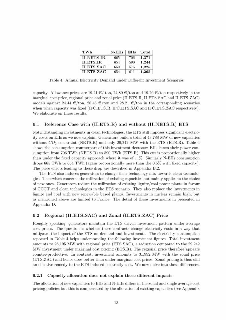
TWh N-EIIs EIIs TotalII NETS IR 665 706 1,371II ETS IR 654 590 1,244II ETS SAC 650 575 1,225II ETS ZAC 654 611 1,265

Table 4: Annual Electricity Demand under Different Investment Scenarios

capacity. Allowance prices are 19.21 e/ ton, 24.80 e/ton and 19.26 e/ton respectively in themarginal cost price, regional price and zonal price (II ETS R, II ETS SAC and II ETS ZAC)models against 24.44 e/ton, 28.48 e/ton and 28.21 e/ton in the corresponding scenarioswhen when capacity was fixed (IFC ETS R, IFC ETS SAC and IFC ETS ZAC respectively).We elaborate on these results.

6.1 Reference Case with (II ETS R) and without (II NETS R) ETS

Notwithstanding investments in clean technologies, the ETS still imposes significant electric-ity costs on EIIs as we now explain. Generators build a total of 43,788 MW of new capacitieswithout CO2 constraint (NETS R) and only 29,242 MW with the ETS (ETS R). Table 4shows the consumption counterpart of this investment decrease: EIIs lessen their power con-sumption from 706 TWh (NETS R) to 590 TWh (ETS R). This cut is proportionally higherthan under the fixed capacity approach where it was of 11%. Similarly N-EIIs consumptiondrops 665 TWh to 654 TWh (again proportionally more than the 0.5% with fixed capacity).The price effects leading to these drop are described in Appendix B.2.

The ETS also induces generators to change their technology mix towards clean technolo-gies. The switch concerns the utilization of existing capacities but mainly applies to the choiceof new ones. Generators reduce the utilization of existing lignite/coal power plants in favourof CCGT and clean technologies in the ETS scenario. They also replace the investments inlignite and coal with new renewable based plants. Investments in nuclear remain high, butas mentioned above are limited to France. The detail of these investments in presented inAppendix D.

6.2 Regional (II ETS SAC) and Zonal (II ETS ZAC) Price

Roughly speaking, generators maintain the ETS driven investment pattern under averagecost prices. The question is whether these contracts change electricity costs in a way thatmitigates the impact of the ETS on demand and investments. The electricity consumptionreported in Table 4 helps understanding the following investment figures. Total investmentamounts to 26,195 MW with regional price (ETS SAC), a reduction compared to the 29,242MW investment under marginal cost pricing (ETS R). The regional price therefore appearscounter-productive. In contrast, investment amounts to 31,992 MW with the zonal price(ETS ZAC) and hence does better than under marginal cost prices. Zonal pricing is thus stillan effective remedy to the ETS induced electricity cost. We now delve into these differences.

6.2.1 Capacity allocation does not explain these different impacts

The allocation of new capacities to EIIs and N-EIIs differs in the zonal and single average costpricing policies but this is compensated by the allocation of existing capacities (see Appendix

13

E for some elaborations). The total renewable and nuclear capacities allocated to EIIs arealmost identical, whether in the regional or zonal price regimes11. The proportion of theother technologies dedicated to EIIs is also similar in both average cost price regimes 12. Thetotals are different though: the capacity dedicated to EIIs amounts to 65,642 MW and 69,758MW respectively in the regional (ETS SAC) and zonal (ETS ZAC) price regimes. This iscompatible with the consumers’ demand reported in Table 4.

6.2.2 National energy policies explain the different impacts

As already observed in the fixed capacity analysis, the regional price entails a drop of con-sumption compared to marginal cost pricing in those zones where nuclear capacity is signif-icant. Investments reinforce these effects. Specifically French EIIs’ consumption decreasesfrom 243 TWh with marginal cost pricing to 176 TWh with the regional price. The reason isthat the regional price reduces the cost of imports of French nuclear electricity by countriesthat cannot invest in that technology. In other words, the regional price forces French EIIsto share national nuclear capacity with foreign industries.

The impact is dramatic: total French nuclear generation for EIIs is 30,492 MW withregional price of which 20,091 MW (66% of total production) supplies domestic EIIs and theremaining 10,400 MW is exported. French electricity prices for EIIs become higher than theaverage of the marginal cost prices of the reference ETS scenario with investments (II ETS R),leading to a 28% cut of EIIs electricity consumption. A similar phenomenon appears at theBelgian node Gramme where industries reduce their power demand by almost 10% under asingle price policy applying with ETS (from 19 TWh in the ETS R model to 18 TWh in theETS SAC case). Contrarily, the regional price is lower than the former marginal cost in theother nodes, because they benefit from these exports at average generation and transmissioncost. To sum up, EIIs’ electricity cost decreases and energy demand increase, at all nodesbut France and Gramme. Together these positive effects are not sufficient to compensate thehigh negative demand variations registered in France and in Gramme. The results is a globalcut of industrial electricity demand of about 2.6% with respect to the reference ETS levels(ETS R)13.

N-EIIs do not do well either in the regional price scenario (ETS SAC). They globallyreduce their power consumption by 1% with respect to the ETS reference case (ETS R) asseen in Table 4. As explained in Appendix F, this is due to the price of allowances.

The situation is altogether different with zonal price where local generators supply EIIs.They increase their global electricity consumption by 4% and 6% with respect to the referenceETS (ETS R) and single (ETS SAC) price scenarios (see Table 4). The drawback is that thisimpact varies locally. French and all Belgian EIIs benefit from the zonal average cost priceand reach a higher level than before the inception of the ETS (NETS R)14. In contrast, thezonal price becomes so expensive in the Dutch locations that EIIs’ power demand becomeslower than in the reference ETS level (ETS R). German EIIs benefit from the zonal price

11Nuclear power plants devoted to EIIs in the ETS SAC amount to 39,423 MW while in the ETS ZAC are39,805 MW, which respectively correspond to the 49% and the 42% of the total dedicated capacity. We havesimilar results also for the renewable capacities: 7,499 MW in the ETS SAC and 7,275 MW in the ETS ZAC.

12In order the capacities dedicated to EIIs are: nuclear, lignite, renewable, coal, CCGT and hydro.13The drop computed with respect to the NETS R amounts to 19%.14EIIs’ demands in France and in the Belgian locations Merchtem and Gramme are 243 TWh, 43 TWh and

21 TWh in the NETS R scenario, while they amount to 254 TWh, 44 TWh and 23 TWh in the ETS ZACcase.

14

system.

6.3 Welfare Analysis

The welfare analysis presented in Table 5 give an alternative view of these phenomena.Investments increase social benefit as seen from Tables 5 and 3. This holds for all cases. The171.58 Billion ewelfare entailed by the zonal price regime (ETS ZAC) is almost identicalto that of the reference ETS case (ETS R) which amounts to 171.72 Billion e. This valueis also the one achieved with the same reference investment case but with fixed capacities(IFC ETS R). All this suggests that the zonal price system with investments effectively andefficiently mitigates the electricity cost induced by the ETS. Note that the N-EIIs’ surpluswith zonal price (ETS ZAC) is almost identical to that in the reference ETS system (ETS R)

Billion e II NETS R II ETS R II ETS SAC II ETS ZACEIIs 20.18 14.68 12.47 15.08N-EIIs 136.97 132.55 130.89 132.56Consumers 157.15 147.23 143.36 147.65

Generators 15.79 23.51 26.09 22.95Allowances 6.90 8.90 6.91

TSO 0.52 0.99 1.21 0.98

Welfare 173.46 171.72 170.66 171.58

Table 5: Welfare under Different Investment Scenarios

The analysis of the EIIs’ and N-EIIs’ surplus reflect demand evolutions. The zonal priceincreases EIIs’ surplus (ETS ZAC) compared to the reference ETS marginal cost scenario(ETS R). Not shown on the table, EIIs’ surplus increases in France and in Belgium overcomesurplus reductions in the remaining locations.

The situation is different under the single price system (ETS SAC), but are again in linewith the observation of the demand. Industries globally reduce both electricity demand andsurplus with respect to the reference ETS case (ETS R) levels. The decrease occurs in Franceand the Belgian Gramme node and is not compensated by the increases a the other locations.

In contrast, generators gain in all ETS scenarios. Line “Generators” of Table 5 reportstheir profits computed by assuming that all allowances needed are fully grandfathered. Prof-its increase with respect to the non ETS reference case (NETS R) by 49%, 65% and 45%respectively in the ETS reference case (ETS R), single price case (ETS SAC) and zonal pricecase (ETS ZAC). The line “Allowances” reports the global allowances costs computed as theproduct of the allowance prices in the different scenarios and the emission cap. The gen-erators’ profits under the hypothesis of full auctioning are simply obtained by subtractingthese allowance values from the corresponding profit reported at line “Generators”. Notethat generators’ profits are higher than before the inception of ETS (NETS R) even with fullauctioning. This phenomenon is explained by the general augment of the electricity prices(at least those paid by N-EIIs) caused by the ETS.

Again, the social welfare includes the TSO’ merchandising profits accruing from the in-troduction of a flow based market coupling organization in transmission.

15

7 Modelling the Combination of the ETS Induced Carbon andthe Electricity Costs (DII)

We now account for the EIIs’ direct carbon costs and participation to the emission market.This is done in two steps. We first expand the cap on allowances to include EIIs’ emissions.Because of lack of information on the separate reactions of the EIIs to electricity and al-lowances prices, we then embed both effects in the EIIs’ electricity demand function. This isdone by adding a carbon component to the price of electricity: the approach is described inAppendix G.

We analyze two different investment scenarios: one without free allowance to industries(hereafter “EIINA”) and one with free allowances (hereafter “EIIA”). The current legislativeproposal for the period after 2012 does not clearly state what the policy towards EIIs willbe. Article 10b of the proposed revision of Directive 2003/87/EC states that Not later thanJune 2011, the Commission shall, in the light of the outcome of the international negotiationsand the extent to which these lead to global greenhouse gas emission reductions, ..., submitto the European Parliament and to the Council an analytical report assessing the situationwith regard to energy-intensive sectors or sub-sectors that have been determined to be ex-posed to significant risks of carbon leakage. This shall be accompanied by any appropriateproposals, which may include: (1) adjusting the proportion of allowances received free ofcharge by those sectors or sub-sectors under Article 10a (compare Section 1); (2) inclusionin the Community scheme of importers of products produced by the sectors or sub-sectorsdetermined in accordance with Article 10a. Any binding sectoral agreements which lead toglobal emissions reductions of the magnitude required to effectively address climate change,and which are monitorable, verifiable and subject to mandatory enforcement arrangementsshall also be taken into account when considering what measures are appropriate.

We assume that the EU acts with the double objective of protecting its industry andmaintaining the overall emission reduction objective. Supposing (for technical reasons) thatEIIs production and electricity consumption are proportional, we further introduce the majorpolicy assumption that free allowances will be allocated proportionally to EIIs’ production(benchmarking policy) and hence to their electricity consumption. This policy fits the objec-tive of protecting EIIs in the international competition. Alternatively, one can also considerthe assumption simply as a first step of the analysis. We calibrate the demand for allowancesand the industrial emission factors on the year 2005 (available at CITL [1]). The data used inthe models of this section are the same as before, except for the introduction of these emissionfactors and the total emission cap, which is increased to 710 Mio ton p.a in order to accountfor EIIs emissions. We concentrate on the joint impact of the special pricing contracts andthe free allowances.

We implemented both the fixed capacity and investment models but, for the sake ofbrevity, only report results with investments. As before, we drop the “DII” model identifierfor results obtained under the assumptions of this section.

Table 6 reports the annual EIIs, N-EIIs’ and total electricity demand in the differentscenarios. The columns “II” recall results obtained in Section 6 with the sole electricitycost. The other columns lists new results obtained by modelling both carbon and electricitycosts under the alternative assumptions that EIIs do not receive (“EIINA”) and receive freeallowances (“EIIA”).

The comparison of the second and following two columns of Table 6 quantify the impactof the carbon cost on EIIs. This points to a very obvious message: adding carbon costs

16

IMPACTS on EIIs IMPACTS on N-EIIs TOTAL DEMANDTWh II DII II DII II DII

EIINA EIIA EIINA EIIA EIINA EIIANETS R 706 665 1,371ETS R 590 517 574 654 657 652 1,244 1,174 1,226ETS SAC 575 492 580 650 656 650 1,225 1,148 1,230ETS ZAC 611 Infeasible 585 654 Infeasible 651 1,265 Infeasible 1,236

Table 6: EIIs and N-EIIs’ Annual Electricity Demand under Different Market Organizations

to electricity costs further reduces EIIs’ activities. The overall decrease can be decomposedin two parts. The move from 706 TWh (II NETS R) to 590 TWh (II ETS R) observedin the second column is the impact of the electricity cost without special contracts andcarbon cost (see Section 6 for more details). Carbon cost without free allowances furtherlowers consumption from 590 TWh (II ETS R) to 517 TWh (ETS R EIINA). Free allowancesgranted in amounts similar to the second phase of the ETS drastically reduce this secondimpact which is now limited to a decrease of demand from 590 TWh (II ETS R) to 574 TWh(ETS R EIIA).

We saw that N-EIIs reduce their electricity demand under the ETS because of higherprices. The burden put on EIIs when there is no free allocation helps N-EIIs recover fromthat situation: the significant demand drop of EIIs’ demand in the reference ETS scenario(ETS R) frees generation capacity and reduces the marginal cost of electricity to N-EIIs.Free allowances eliminate this recovery of N-EIIs. The results confirm that free allowancesmitigate the impact of carbon cost on EIIs. They also reveal an impact on N-EIIs.

It remains to examine whether special contracts still mitigate the impact of the electricitycost on EIIs. The outcome is mixed and, as shown in Table 6, can even be extreme. A com-bination of zonal pricing and full auctioning (ETS ZAC EIINA) makes the model infeasible,implying that it is impossible to meet the environmental target without free allowances forEIIs15. The special price contracts are only productive under free allowances; zonal pricesthen do better than regional prices. We elaborate on these findings.

7.1 Reference Case with (DII ETS R) and without (DII NETS R) ETS:Full Auctioning (EIINA) and Free Allowances (EIIA)

The addition of the carbon cost to electricity cost without a compensation through free al-lowances further reduces EIIs’ demand from 590 TWh (II ETS R) to 517 TWh (ETS R EIINA).All zones contribute to the decrease. Investments reduce from 29,242 MW in the referenceETS case with the sole electricity costs (II ETS R), to 14,921 MW with both carbon andelectricity costs (ETS R EIINA), no allowance and no special price contract (compare Tables10 and 11 in Appendix H). The price of allowances is also low and equal to 12.45 e/ton,which encourages the use of existing coal capacity. Free allowances significantly mitigate theimpact of carbon cost on EIIs. Industrial demand only decreases from 590 TWh (II ETS R)to 574 TWh (ETS R EIIA). In this last case, investments amount to a total of 30,338 MWbecause of a combined effect of demand increase and capacity restructuring (see Table 12 inAppendix H). The allowance price increases to 22.26 e/ton and induces investing in clean

15Feasibility is reached by relaxing the emission constraints and indirectly the amount of allowances theyhave to pay for.

17

technologies and scrapping existing coal capacities. This also increases N-EIIs’ prices anddecreases their consumption compared to the other reference cases in Table 616. Notwith-standing this improvement EIIs do not recover the position observed with the sole electricitycosts.

To sum up the granting of free allowances in proportion to production, that is accordingto a benchmark policy effectively compensates for carbon costs.

7.2 Regional Price (DII ETS SAC): Full Auctioning (EIINA) and FreeAllowances (EIIA)

7.2.1 Full auctioning (EIINA)

A regional price (ETS SAC) with full auctioning of allowances does not help EIIs. We arguedin Section 6.2 devoted to the sole electricity cost that the regional price reduces consumptionfrom 590 TWh (II ETS R) to 574 TWh (II ETS SAC) and that the diversity of nationalenergy policies explains this counter-productive effect. The application of a regional price toa market with both carbon and electricity costs and no free allowances similarly decreasesEIIs’ demand from 517 TWh (ETS R) to 492 TWh (ETS SAC). In short, EIIs suffer notonly from both carbon and electricity costs but also from the counter-productive effect ofthe intended (regional price) remedy. The explanation is similar to the one of Section 6.2:a regional price applied on diverging energy policies subsidizes exports of nuclear energy byreducing the transmission costs of that export. This deprives French EIIs from the benefits ofdomestic nuclear developments. French EIIs consumption drops from 211 TWh in the puremarginal cost pricing (ETS R) to 152 TWh (ETS SAC) with the regional price. BelgianEIIs’ consumption similarly drops in Gramme from 17 TWh to 15 TWh between these twoscenarios. As in Section 6.2, the regional price (ETS SAC) benefit EIIs in the remaininglocations, with respect to the corresponding reference case. Altogether the rises do notcompensate French and Belgian losses.

A by-product is that N-EIIs benefit from the regional price. Decreasing consumptionlowers the allowance price to 14.71 e/ton (ETS SAC) and hence also the marginal cost ofelectricity to N-EIIs. These increase their consumption with respect to the levels computedwith the regional price when only accounting for electricity cost (II ETS SAC)17.

Finally, the reduced EIIs’ demand of electricity and low allowance price affect investments.These reduce to 8,927 MW with a regional price without free allowances (ETS SAC EIINA)MW (see Table 11), -66% less than with the sole electricity costs (II ETS SAC).

7.2.2 Free allowances (EIIA)

Free allowances improve the picture: EIIs electricity demand increases from 574 TWh withmarginal cost pricing (ETS R EIIA) to 580 TWh with regional price (ETS SAC EIIA). Thislooks like a marginal variation, but it is significant when compared to the application of theregional price with full auctioning where EIIs demand was 492 TWh Again, French EIIs have

16Like in the other reference investment cases in Table 6, coal and CCGT plants define the N-EIIs’ summerand winter electricity prices in the DII ETS R EIIA model. N-EIIs’ demand falls is summer are 0.3% and 1%with regard to the II ETS R and the DII ETS R EIINA cases, while in winter are respectively of 0.3% and0.7%.

17Note that both in the II ETS SAC and the DII ETS SAC EIINA models, coal and CCGT plants define N-EIIs’ electricity prices in summer and in winter respectively. Considering the marginal cost pricing approach,a lower allowance price reduce also electricity price if fuel charges do not change.

18

to give up some of the benefit of domestic nuclear capacities because of a pricing system thatsubsidizes exports. The same happens in the Belgian node Gramme. This implies that thedecrease of French consumption is drastic, even though smaller in Gramme. These decreasesare barely compensated by the increases in other countries18 but the net result is this timepositive.

N-EIIs, which do not incur direct carbon costs, roughly maintain their consumption withrespect to the regional price scenario computed with the sole electricity cost (II ETS SAC)(see Tables 6). The key element here is the is allowance price, which at 24.80 e/ton remainsthe same in both scenarios and adds to coal and CCGT fuel costs to set the electricity pricefor N-EIIs.

Finally, investments in new capacity totally amount to 29,544 MW, a much higher valuethan with full auctioning (compare Tables 11 and 12 in Appendix H). This again results froma joint demand increase and technology restructuring effect due to the high allowance price.

7.3 Zonal price (DII ETS ZAC): Full Auctioning (EIINA) and Free Al-lowances (EIIA)

The combination of zonal prices, carbon cost and full auctioning makes the model infeasible:the market cannot meet the reduction target. Free allowances restore the situation. EIIsincrease their activity with respect to various other situations as can be seen from the resultsof Table 6. The increase of demand from 574 TWh with marginal cost pricing and freeallowances (ETS R EIIA) to 585 TWh with zonal prices and free allowances (ETS ZAC EIIA)indicates that this policy mix partially remedies the demand lost because of the electricitycost. But this recovery is small: one can measure the loss incurred by EIIs as a result ofthe ETS after compensation with free allowances by the drop of demand from 706 TWh(II NETS R) to 574 TWh (ETS R EIIA). A recovery of 11 TWh is only 8% of that amount.The reason again lies in the diversity of energy policies, which this time operates as follows:French and all Belgian industries increase their electricity demand compared to the referencecase ETS R EIIA because of their access to the nuclear and new renewable capacities; butEIIs’ consumption in the other nodes falls because they miss this access.

This larger electricity demand increases the allowance price. It amounts to 24.76 e/tonagainst the 22.26 e/ton in the corresponding reference case with free allowances (ETS R EIIA).The combination of these demand and allowance price effects in turn increases investmentwhich now amount to 32,957 MW

As before, the higher allowance price slightly increases N-EIIs’ electricity prices comparedto the reference marginal cost case (ETS R)19: N-EIIs’ consumption falls by -0.2% (see Tables6).

7.4 Welfare Analysis

Tables 7 and 8 report the surpluses/profits of the market players when allowances are respec-tively fully auctioned and are given for free. We report the EIIs’ gross and the net surpluses,that are before and after accounting for allowance payments respectively. The allowance val-ues are indicated in line “Allowances (EIIs)”. Note that by construction, in the EIINA model,

18In absolute values, the fall of the French industrial demand is from 240 TWh in the ETS R EIIA to 174TWh in the ETS SAC EIIA. In Gramme, the EIIs’ demand drop is from 20 TWh to 19 TWh.

19Again, coal and CCGT defines their periodical prices both in the DII ETS R EIIA and in theDII ETS ZAC EIIA. The difference between the two models is still represented by allowance price.

19

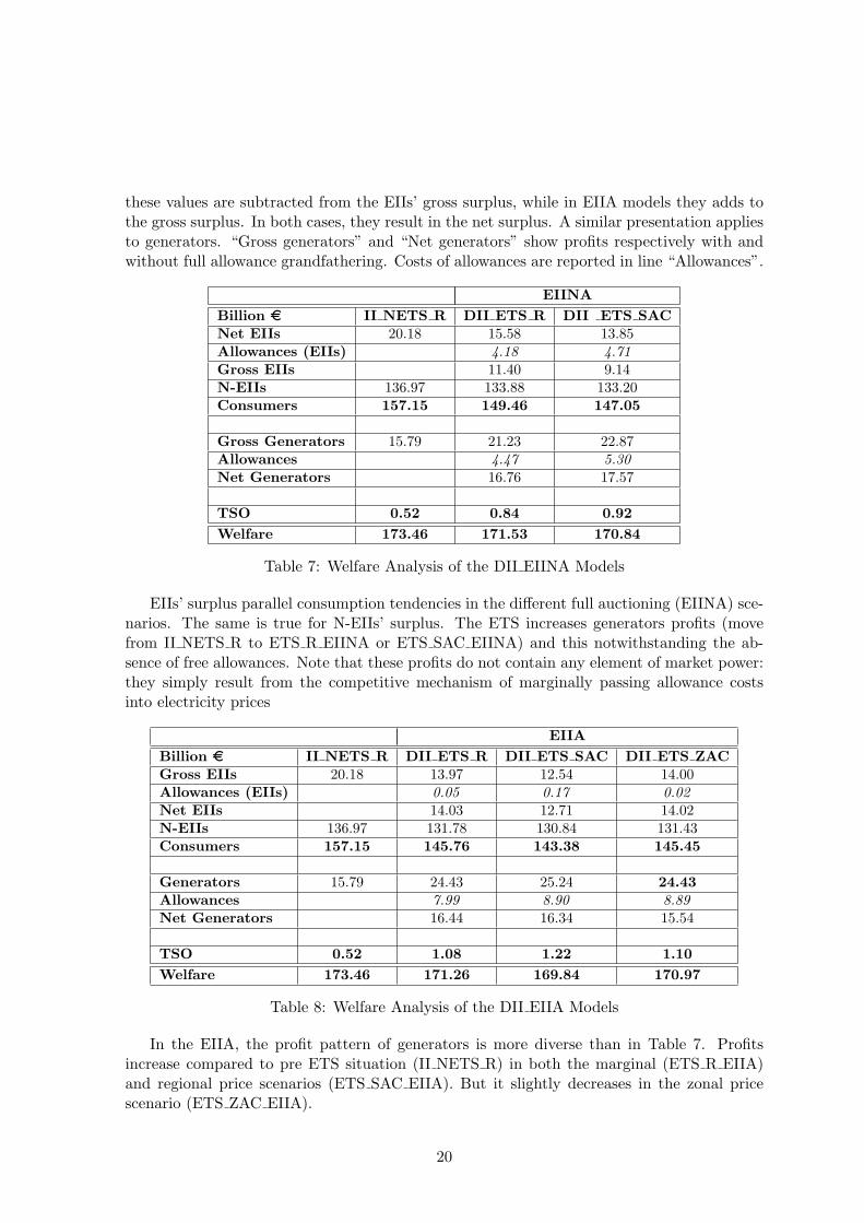
these values are subtracted from the EIIs’ gross surplus, while in EIIA models they adds tothe gross surplus. In both cases, they result in the net surplus. A similar presentation appliesto generators. “Gross generators” and “Net generators” show profits respectively with andwithout full allowance grandfathering. Costs of allowances are reported in line “Allowances”.

EIINABillion e II NETS R DII ETS R DII ETS SACNet EIIs 20.18 15.58 13.85Allowances (EIIs) 4.18 4.71Gross EIIs 11.40 9.14N-EIIs 136.97 133.88 133.20Consumers 157.15 149.46 147.05

Gross Generators 15.79 21.23 22.87Allowances 4.47 5.30Net Generators 16.76 17.57

TSO 0.52 0.84 0.92Welfare 173.46 171.53 170.84

Table 7: Welfare Analysis of the DII EIINA Models

EIIs’ surplus parallel consumption tendencies in the different full auctioning (EIINA) sce-narios. The same is true for N-EIIs’ surplus. The ETS increases generators profits (movefrom II NETS R to ETS R EIINA or ETS SAC EIINA) and this notwithstanding the ab-sence of free allowances. Note that these profits do not contain any element of market power:they simply result from the competitive mechanism of marginally passing allowance costsinto electricity prices

EIIABillion e II NETS R DII ETS R DII ETS SAC DII ETS ZACGross EIIs 20.18 13.97 12.54 14.00Allowances (EIIs) 0.05 0.17 0.02Net EIIs 14.03 12.71 14.02N-EIIs 136.97 131.78 130.84 131.43Consumers 157.15 145.76 143.38 145.45

Generators 15.79 24.43 25.24 24.43Allowances 7.99 8.90 8.89Net Generators 16.44 16.34 15.54

TSO 0.52 1.08 1.22 1.10Welfare 173.46 171.26 169.84 170.97

Table 8: Welfare Analysis of the DII EIIA Models

In the EIIA, the profit pattern of generators is more diverse than in Table 7. Profitsincrease compared to pre ETS situation (II NETS R) in both the marginal (ETS R EIIA)and regional price scenarios (ETS SAC EIIA). But it slightly decreases in the zonal pricescenario (ETS ZAC EIIA).

20

8 Conclusion

We analyse policies consisting of a mix of free allowances and special electricity contracts forEIIs. We find that special full cost based pricing contracts help relieve the electricity costsimposed by the ETS on EIIs. But the benefits of these contracts are hampered by differencesof national energy policies. The regional price helps EIIs located in non nuclear countries andthe opposite is true for the zonal contracts. All in all, zonal prices seem to do better. This isto some extent not surprising because the regional price system embeds a subsidizing effectthat can only be detrimental to efficiency. Zonal prices may not look like an internal marketsolution but the regional price, with its subsidizing effects, is a false internal market solution.The differences as to who gains and who looses in the different policies and the willingness tomaintain national policies suggest that it will be difficult to arrive at an harmonized solutionin the EU.

The situation is clearer for free allowances. As expected they always help EIIs recovertheir carbon costs, at least when applied as here on a benchmarking basis. The difficulty isthus to get the benchmarking principle accepted at the EU level.

N-EIIs are generally loosing in the adventure. They remain priced at marginal cost andhence suffer from higher allowances cost than EIIs which pay them at average cost. Moreover,the higher the success of the EIIs policy is, the higher the allowance price and hence theelectricity price to N-EIIs.

This analysis does not take any position on the importance of carbon leakage. It simplypoints to problems that could arise were this phenomenon important. It is indeed particularlyworrying to note that it is extremely difficult to find quantitative information about thereality of the phenomenon and the reaction of the EIIs to electricity an carbon costs. A mainconclusion of the analysis is thus to draw the attention to the fact that we need to understandthese reactions much better than is the case today. A last comment is the crucial importanceof nuclear policy. Renewable and nuclear are key players in the policies investigated here.But we probably cannot afford to only rely on subsidized renewable.

References

[1] Community Independent Transaction Log. 2006.http : //ec.europa.eu/environment/climat/emission/citl en.htm

[2] Davis, K., URS Corporation. 2003. Greenhouse Gas Emission Factor Review. EdisonMission Energy.

[3] Delgado, J. 2007. Why Europe is not Carbon Competitive?. Bruegel Policy Brief. 5.

[4] Demailly, D., P. Quirion. 2006. CO2 abatement, competitiveness and leakage in theEuropean cement industry under the EU-ETS: grandfathering versus output-based al-location. Climate Policy. 6 93–113.

[5] Dirkse, S.P., M.C. Ferris. 2000. Complementarity Problems in GAMS and the PATHsolver. Journal of Economic Dynamics and Control. 24(2) 165–188.

[6] Duthaler C., M. Emery, G. Andersson, M. Kurzidem. 2008. Analysis of the use of PTDFin the UCTE Transmission Grid, presented at Power Systems Computation Conference,Glasgow, July 2008.

21

[7] ECN. 2005. Evaluation of models for market power in electricity networks Test data.Retrieved March, 2005, http : //www.ecn.nl/en/ps/products−services/models−and−instruments/competes/model − evaluation/.

[8] Hidalgo, I., L. Szabo, J. C. Ciscar, A. Soria. 2005. Technological prospects and CO2

emission trading analyses in the iron and steel industry: A global model Energy. 30583–610.

[9] Hourcade, J.C., D. Demailly, K. Neuhoff, M. Sato. 2008. Differentiation and dynamicsof the EU ETS competitiveness impacts. Climate Strategy Report.

[10] McKinsey&Company. May 2007. Curbing Global Energy Demand Growth: The EnergyProductivity Opportunity. McKinsey Global Institute.

[11] Newbery, D. M. 2003. Sectoral dimensions of sustainable development: energy and trans-port. Economic Survey of Europe. 2 73–93.

[12] Oggioni, G., Y. Smeers. 2008. Evaluating the Impact of Average Cost Based Contractson the Industrial Sector in the European Emission Trading Scheme. CORE DiscussionPaper. 01.

[13] Oggioni, G., Y. Smeers. 2008. An Electricity Market Equilibrium Model with AlternativeEnergy Pricing Regimes. In preparation.

[14] Perekhodtsev, D. 2008. Assessment of geographic scope of electricity markets: the case offlow-based market coupling, presented at “The Economics of Energy Markets”, Toulouse,June 2008.

[15] Pizer, W. A. 2008 in The Design of Climate Policy, Guesnerie, R. and H. Tulkens ed.,201–216, MIT Press. Forthcoming.

[16] Szabo L., I. Hidalgo, J. C. Ciscar, A. Soria. 2006. CO2 emission trading within theEuropean Union and Annex B countries: the cement industry case. Energy Policy. 3472–87.

[17] Zhou, Q., J.W. Bialek. 2005. Approximate model of European interconnected system asa benchmark system to study effects of cross-border trades. IEEE Transaction on PowerSystem, 20(2) 782–788.

Appendix A: Underlying Mathematical Techniques and theirImplementations

Our models are formulated as complementarity problems. More specifically, given a cone Kand a mapping F : K → Rn, the complementarity problem, denoted by CP (K,F ) is to finda nonnegative vector x ∈ Rn satisfying the following condition:

0 ≤ F (x)⊥x ≥ 0 (1)

where F (x) is assumed to be nonnegative. The use of the term “complementarity” derivesfrom the concept of orthogonality (⊥) stated in the definition. In fact, the scalar productF (x) · x equals zero.

22

Complementarity based models offer a natural approach to construct partial and generalequilibrium problems where several market agents interact together. In our specific case,we consider the generators, the consumers and the TSO. Their complementarity models areobtained by computing the KKT conditions of their optimization models and matching themwith the associated primal and dual variables.

Generators solve two different pricing models in accordance with the electricity pricingscenario considered. In the reference case, representing a perfectly competitive market, gen-erators are (energy and transmission) price takers and maximize their profits accruing fromselling electricity to both consumer segments. In doing that, they have to account for thecapacity constraint of their power plants.

In the leakage mitigation scenarios, generators maximize their profit when selling to N-EIIs and minimize the cost of supplying EIIs. This different optimization approach is a directconsequence of the application of average cost prices which do not lead to maximize profits.However, generators are charged in the same way for transmission on both segments.

This has also some mathematical implications. While our perfectly competitive opti-mization model defines a convex problem and has a global solution, the average cost pricingscenarios introduce non- convexity20 that may lead to either a multiplicity of disjoint equi-libria or no equilibrium. Apart from a very difficult case in the third stage of our analysis,our average cost pricing models have several disjoint solutions21.

In any pricing scenarios, EIIs and N-EIIs maximize their surpluses. In addition, ourmodels account for the energy market balance, the transmission and the emission constraints.

The final complementarity problems are obtained by assembling together the KKT con-ditions of the market agents’ optimization problems and the market clearing relations. Thisset of complementarity problems are solved in GAMS by PATH as explained by Dirkse andFerris [5].

Appendix B: Pricing Effects in the Reference Cases with andwithout ETS

Appendix B.1. With Fixed Capacities

The introduction of the carbon market has a dual effect on the seasonal marginal prices ofelectricity. Summer prices increase in IFC ETS R compared to IFC NETS R. We observethat the same coal plant set the price of electricity at the hub both in the IFC NETS R andIFC ETS R models. But in IFC ETS R, generators pass the allowance (opportunity) costsin the electricity prices which thus increases the price paid by EIIs and N-EIIs. The resultis opposite in winter where prices decrease under the ETS. The cause is the EIIs’ demanddecrease which eliminates the most emitting plants from the merit order: generators useboth old single cycle natural gas and oil-fired power plants in the IFC NETS R scenario,which entail a high electricity price. These highly emitting plants are abandoned in theETS where CCGT power stations become marginal. This decreases the price of electricity.The combination of a lower price and a lower demand may look counter-intuitive, but it isexplained by the imposed equality of EIIs power demand in both the summer and winter. Itis not the lower winter price that induces the lower EIIs’ demand, but the combination of a

20Non-convexity corresponds to non-monotonicity in the complementarity problems.21We obtained different results by setting different starting points for the algorithm.

23

higher summer price and a lower winter price that implies a lower demand in both summerand winter. The ETS introduces some changes in technology mix used to produce electricitywith a consequent modification of the electricity prices. In particular, in the ETS R scenarioswith carbon restrictions, this interpretation is confirmed by the more intuitive behaviour of N-EIIs. There is no inter–seasonal link of consumption for these consumers. They accordinglyincrease their consumption by 1% in the winter period in the IFC ETS R scenario whereprices are a little bit lower in each node than in the IFC NETS R scenario. In summer,instead, they reduce their energy utilization by almost 3% as a consequence of the higherpower prices. The decrease of the summer N-EIIs’ demand prevails on the correspondingwinter increase and this results in a global N-EIIs’ demand reduction as indicated in Table2. The phenomenon globally illustrates that generators’ capability to transfer their carboncosts in the final price paid by consumers is limited in the long-term if the reaction of theEIIs is important.

Appendix B.2. With Investments

Increases of electricity prices cause these global demand fall: coal and CCGT power plants setthe marginal electricity prices respectively in summer and in winter both with and withoutthe ETS. The marginal cost prices then increase because of the additional carbon cost impliedby the ETS.

Appendix C: Impact of Investments on Electricity Demand ofthe Reference Case with and without ETS

The comparison of the data reported in Tables 2 and 4 shows that, in the absence of the ETSand with investments (II NETS R) EIIs increase their demand by 18% compared to the casewith fixed capacities (IFC NETS R), that is, an increase from 598 TWh to 706 TWh. N-EIIs’increase is about +2% (from 649 TWh to 665 TWh). This positive tendency is also confirmedby the couple II ETS R and IFC ETS R: with investments and ETS, EIIs augment theirelectricity consumption by 11% (from 531 TWh to 590 TWh) compared to the applicationof the ETS with fixed capacities. N-EIIs raise their energy demand by 1% (from 646 TWhto 654 TWh).

Appendix D: Discussion of Investments Patterns in the “II”scenarios

Among the 43,788 MW of new capacities invested without ETS (II NETS R), 17,799 MW(41%) are nuclear in France, 18,570 MW (42%) lignite in Germany and 7,419 MW (17%)coal distributed between Belgium and the Netherlands. With the 29,242 MW of new capacityinvested with ETS (II ETS R), 26,641 MW (91%) are new nuclear plants in France and theremaining 2,600 MW (9%) are renewable in Belgium. Generators choose these locationsfor different reasons. As already said, France is the unique country in the model that allowsinvestments in nuclear; new renewable stations happen to be, in our input data, less expensiveto build in Belgium than in the other countries. Moreover, because of their high capacitycosts and limited availability, there are no investments in hydro plants.

24

Appendix E: Capacity allocation in the II ETS SAC and in theII ETS ZAC Models

Generators reserve 29,533 MW of the 31,992 MW invested under the zonal pricing policy(II ETS ZAC) to N-EIIs of which 1,620 MW are renewable plants in Belgium and 27,913MW are nuclear power stations in France. Investments for EIIs are only 2,458 MW of newrenewable plants built in Belgium. In contrast, in the single price regime (II ETS SAC),17,400 MW of investment go to EIIs and 8,796 are for N-EIIs. Again, these are nuclear(in France) and renewable (in Germany and in Belgium) power stations that, this time, arereserved both to EIIs and N-EIIs.

This allocation of new capacities implies that EIIs are mainly supplied by existing plantsand one indeed observes that the allocation of the existing renewable and nuclear capacitiesfollows an opposite pattern in the two average cost pricing models.

In both the regional and zonal models, old gas and oil existing plants are reserved forN-EIIs but are never used even in winter. These plants should thus be scrapped. We alsoobserve that in both average cost pricing scenarios, part of the N-EIIs’ old or new Frenchnuclear capacities remains idle in summer because total capacity exceeds demand and networkcongestion does not allow more export of nuclear energy.

Appendix F: Allowance Prices in the “II” Scenarios

The increase of the allowance price from 19.21 e/ton in the reference ETS case to 24.80 e/tonunder single price (respectively II ETS R and II ETS SAC) explains the N-EIIs’ consumptiondecrease: the higher allowance price affects the same coal and CCGT plants that set N-EIIs’marginal prices in summer and in winter in both scenarios and hence increases electricityprices. The smaller investment in clean technologies, caused by the drop of investment, andhence the increased utilization of fossil plants in turn explain the raise of allowance price.

As argued before, new investments are mainly dedicated to N-EIIs in the zonal pricing sys-tem while EIIs are supplied by existing capacities. The two nodes with investments are thuslargely exporting to N-EIIs. This especially holds for France where old and new nuclear pro-vides 77% of the electricity generated at the node and covers the 92% of the power exported.This benefit N-EIIs that recover their ETS reference level of 654 TWh, notwithstanding theglobal increased consumption of the EIIs.

Appendix G: Modelling the Direct ETS Impact

The following requires introducing an assumption of proportionality between emissions andelectricity consumption (linear technology). It expresses that EIIs’ emissions depend onproduction levels that, in turn, determine electricity consumption. Because of the lack infor-mation, we consider the whole EIIs sector as one firm. This restriction is not methodologicaland it can be relieved with sectoral data. Let π denote the profit function of this aggregatefirm. We want to study its reaction to changes of both the electricity and allowance pricesand include both effects in the sole demand function. The profit π is stated as:

π = py · y − pe · e− po · o− pco2 · co2 (2)

25

which is interpreted as follows. Industries’ revenues accrue from selling output y at price py.They consume non electricity inputs o and electricity e to produce output y. Let po and pebe the prices of these inputs. Industries incur a cost pco2 for each allowance bought on themarket; co2 is the net purchase, that is the amount of emissions reduced by the allowancesreceived for free.

Introducing the policy assumption that free allowances are granted proportionally toproduction and the technological assumption that the amount of electricity e, allowances co2and input o vary as a function of production we can write:

• e = α · y

• co2 = (β − γ) · y

• o = ϕ(y)

where α represents the unit electricity consumption (a technical parameter), β is the emissionfactor per unit of output y (a technical parameter) and γ is the proportion of free allowancesreceived by unit y (a policy parameter). ϕ(y) is the consumption of non electricity input as afunction of the output y. Recall that we stated a linear dependence between the demand ofenergy e and allowances co2 and the industrial production y (again this is not a methodologicallimitation) but for reason that will be clear later in the section, we allow for a slightly moregeneral treatment of the consumption of non electricity input ϕ(y)

We can then write (2) as a function of the sole output y and obtain:

π(y) = py · y − pe · α · y − pco2 · (β − γ) · y − po · ϕ(y) (3)

We arrive at the industrial demand of electricity by computing the First Order Conditions(FOC) of (3) with respect to y and obtain:

∂π

∂y= py − pe · α− pco2 · (β − γ)− po · ϕ′(y) = 0 (4)

Our objective is to separately get hold of the electricity price (pe), which measures the indirectETS costs and of the allowance price (pco2) which determines the direct carbon cost. We thenre-write condition (4) as follows:

pe · α+ pco2 · (β − γ) = py − po · ϕ′(y) (5)

By dividing by α on the left and right hand sides of equation (5), one gets:

pe + pco2 · (β − γα

) =1α

[py − po · ϕ′(y)

](6)

which has the form of a demand function: the left hand side is a combination of the electricityand allowance prices which has the dimension of a euro/MWh while the right hand side isonly a function of the output of the firm (the price of the output is fixed in this partialequilibrium model). Because we are assuming linear demand functions throughtout, we nowimpose the particular functional form ϕ

′(y) = a+ b · y and write:

pe + pco2 · (β − γα

) =1α

[py − po · (a+ b · y)] (7)

26

Using the relation e = α · y, we substitute y in (7) and obtain:

pe + pco2 · (β − γα

) = py1α− po

a

α− po

b

α2e (8)

By setting A = py1α − po

aα and B = po

bα2 , we have:

pe + pco2 · (β − γα

) = A−Be (9)

This is the intended demand function. Equation (9) represents the industrial demand ofelectricity, where pe and e are respectively the EIIs’ electricity price and demand. It includesalso the emission allowance price pco2 multiplied by the factor (β−γα ) which defines the impactof the application of different emission policies on EIIs. This demand function allows one toconsider different scenarios of free allowances to the EIIs such as:

1. full grandfathering of allowances (β = γ). This is in line with the situation prevailingin the 2005-2007 ETS phase;

2. Full auctioning of allowances (γ = 0). This is what is foreseen for the period after 2012by the proposed revision of the ETS Directive;

3. Partial grandfathering of allowances (β 6= γ). This is a more general situation which canrepresent a declining free allowance policy for EIIs or a full free allocation as foreseen bythe proposed new ETS Directive in case industries become too exposed to internationalcompetition.

As mentioned before, we limit the analysis to two contrasted scenarios. We first considerthe case of full auctioning which is modelled by setting the value of γ to zero. The factor(β−γα ) becomes (βα), which is an emission factor that we compute on the basis of 2005 dataavailable at CITL [1]. We refer to this case as “EIINA”. We also consider the scenario “EIIA”where industries receive a proportion of free allowances. In this scenario, we have the factor(β−γα ) to which we refer as “allowance factor”. Both approaches are compatible with theproposed revision of the ETS Directive. The emission component of the electricity price ispco2 ·

βα in the EIINA models and pco2 ·

β−γα in the EIIA scenarios. The EIIs’ demand for

allowances is:allowance demand =

β − γα· e

The inclusion of the emission/allowance in the industrial electricity demand modifies EIIs’electricity consumption that now depends on both the power and carbon prices.

Appendix H: Investments and Capacity Allocations

Table 13 report the EIIs’ demands when nuclear investments are unconstrained. EIIs’ demandis identical in the II NETS R and in the II ETS R scenarios. The reason is that emissionconstraint is not binding and hence the EIIs’ demand is set by nuclear marginal cost in bothcases. The situation changes when carbon cost is included in the model. Emission constraintbecomes active at low allowance price. Still EIIs must pay for them, which change theirdemand. This effect disappears with free allowances (see Table 13).

27

Available CapacityMW Germany France Merchtem Gramme Krimpen Maastricht Zwolle TotalHydro 1,505 6,084 0 13 0 0 0 7,602Renewable 4,584 0.95 20 21 101 101 101 4,930Nuclear 15,007 45,369 2,078 2,204 337 0 0 64,995Lignite 17,783 77 0 0 0 0 0 17,860Coal 24,613 8,824 1,564 979 3,128 0 482 39,590CCGT 13,544 8,164 2,589 1,207 4,432 2,917 4,834 37,687Old gas 2,147 256 194 170 833 3,600Oil based 4,760 55 194 5,009Total 79,183 73,535 6,500 4,788 8,831 3,018 5,417 181,273

Table 9: Available Capacity by Node in MW

MW CAPACITYExisting Investments Total

II NETS R 181,273 43,787 225,060II ETS R 181,273 29,242 210,515II ETS SAC 181,273 26,195 207,468II ETS ZAC 181,273 31,991 213,264

Table 10: Total Capacity in the II Scenarios

MW CAPACITYExisting Investments Total

DII ETS R EIINA 181,273 14,921 196,194DII ETS SAC EIINA 181,273 8,927 190,200DII ETS ZAC EIINA Infeasible Infeasible Infeasible

Table 11: Total Capacity in the DII Scenarios with Full Auctioning EIINA

MW CAPACITYExisting Investments Total

DII ETS R EIIA 181,273 30,338 211,611DII ETS SAC EIIA 181,273 29,544 210,817DII ETS ZAC EIIA 181,273 32,957 214,230

Table 12: Total Capacity in the DII Scenarios with Free Allocation EIIA

TWh II DIIEIINA EIIA

NETS R 789ETS R 789 777 791ETS SAC 777 764 779ETS NAC 781 768 783

Table 13: EIIs’ Electricity Demand Under Different Nuclear Investment Scenarios

28

Recent titles CORE Discussion Papers

2008/23. Marco MARINUCCI. Optimal ownership in joint ventures with contributions of asymmetric

partners. 2008/24. Raouf BOUCEKKINE, Natali HRITONENKO and Yuri YATSENKO. Optimal firm behavior

under environmental constraints. 2008/25. Ana MAULEON, Vincent VANNETELBOSCH and Cecilia VERGARI. Market integration in

network industries. 2008/26. Leonidas C. KOUTSOUGERAS and Nicholas ZIROS. Decentralization of the core through

Nash equilibrium. 2008/27. Jean J. GABSZEWICZ, Didier LAUSSEL and Ornella TAROLA. To acquire, or to compete?

An entry dilemma. 2008/28. Jean-Sébastien TRANCREZ, Philippe CHEVALIER and Pierre SEMAL. Probability masses

fitting in the analysis of manufacturing flow lines. 2008/29. Marie-Louise LEROUX. Endogenous differential mortality, non monitored effort and optimal

non linear taxation. 2008/30. Santanu S. DEY and Laurence A. WOLSEY. Two row mixed integer cuts via lifting. 2008/31. Helmuth CREMER, Philippe DE DONDER, Dario MALDONADO and Pierre PESTIEAU.

Taxing sin goods and subsidizing health care. 2008/32. Jean J. GABSZEWICZ, Didier LAUSSEL and Nathalie SONNAC. The TV news scheduling

game when the newscaster's face matters. 2008/33. Didier LAUSSEL and Joana RESENDE. Does the absence of competition in the market foster

competition for the market? A dynamic approach to aftermarkets. 2008/34. Vincent D. BLONDEL and Yurii NESTEROV. Polynomial-time computation of the joint

spectral radius for some sets of nonnegative matrices. 2008/35. David DE LA CROIX and Clara DELAVALLADE. Democracy, rule of law, corruption

incentives and growth. 2008/36. Jean J. GABSZEWICZ and Joana RESENDE. Uncertain quality, product variety and price

competition. 2008/37. Gregor ZOETTL. On investment decisions in liberalized electricity markets: the impact of price caps at the spot market.

2008/38. Helmuth CREMER, Philippe DE DONDER, Dario MALDONADO and Pierre PESTIEAU. Habit formation and labor supply.

2008/39. Marie-Louise LEROUX and Grégory PONTHIERE. Optimal tax policy and expected longevity: a mean and variance approach.

2008/40. Kristian BEHRENS and Pierre M. PICARD. Transportation, freight rates, and economic geography.

2008/41. Gregor ZOETTL. Investment decisions in liberalized electricity markets: A framework of peak load pricing with strategic firms.

2008/42. Raouf BOUCEKKINE, Rodolphe DESBORDES and Hélène LATZER. How do epidemics induce behavioral changes?

2008/43. David DE LA CROIX and Marie VANDER DONCKT. Would empowering women initiate the demographic transition in least-developed countries?

2008/44. Geoffrey CARUSO, Dominique PEETERS, Jean CAVAILHES and Mark ROUNSEVELL. Space-time patterns of urban sprawl, a 1D cellular automata and microeconomic approach.

2008/45. Taoufik BOUEZMARNI, Jeroen V.K. ROMBOUTS and Abderrahim TAAMOUTI. Asymptotic properties of the Bernstein density copula for dependent data.

2008/46. Joe THARAKAN and Jean-Philippe TROPEANO. On the impact of labor market matching on regional disparities.

2008/47. Shin-Huei WANG and Cheng HSIAO. An easy test for two stationary long processes being uncorrelated via AR approximations.

2008/48. David DE LA CROIX. Adult longevity and economic take-off: from Malthus to Ben-Porath. 2008/49. David DE LA CROIX and Gregory PONTHIERE. On the Golden Rule of capital accumulation

under endogenous longevity.

Recent titles CORE Discussion Papers - continued

2008/50. Jean J. GABSZEWICZ and Skerdilajda ZANAJ. Successive oligopolies and decreasing returns. 2008/51. Marie-Louise LEROUX, Pierre PESTIEAU and Grégory PONTHIERE. Optimal linear taxation

under endogenous longevity. 2008/52. Yuri YATSENKO, Raouf BOUCEKKINE and Natali HRITONENKO. Estimating the dynamics

of R&D-based growth models. 2008/53. Roland Iwan LUTTENS and Marie-Anne VALFORT. Voting for redistribution under desert-

sensitive altruism. 2008/54. Sergei PEKARSKI. Budget deficits and inflation feedback. 2008/55. Raouf BOUCEKKINE, Jacek B. KRAWCZYK and Thomas VALLEE. Towards an

understanding of tradeoffs between regional wealth, tightness of a common environmental constraint and the sharing rules.

2008/56. Santanu S. DEY. A note on the split rank of intersection cuts. 2008/57. Yu. NESTEROV. Primal-dual interior-point methods with asymmetric barriers. 2008/58. Marie-Louise LEROUX, Pierre PESTIEAU and Gregory PONTHIERE. Should we subsidize

longevity? 2008/59. J. Roderick McCRORIE. The role of Skorokhod space in the development of the econometric

analysis of time series. 2008/60. Yu. NESTEROV. Barrier subgradient method. 2008/61. Thierry BRECHET, Johan EYCKMANS, François GERARD, Philippe MARBAIX, Henry

TULKENS and Jean-Pascal VAN YPERSELE. The impact of the unilateral EU commitment on the stability of international climate agreements.

2008/62. Giorgia OGGIONI and Yves SMEERS. Average power contracts can mitigate carbon leakage.

Books Y. POCHET and L. WOLSEY (eds.) (2006), Production planning by mixed integer programming. New York,

Springer-Verlag. P. PESTIEAU (ed.) (2006), The welfare state in the European Union: economic and social perspectives.

Oxford, Oxford University Press. H. TULKENS (ed.) (2006), Public goods, environmental externalities and fiscal competition. New York,

Springer-Verlag. V. GINSBURGH and D. THROSBY (eds.) (2006), Handbook of the economics of art and culture.

Amsterdam, Elsevier. J. GABSZEWICZ (ed.) (2006), La différenciation des produits. Paris, La découverte. L. BAUWENS, W. POHLMEIER and D. VEREDAS (eds.) (2008), High frequency financial econometrics:

recent developments. Heidelberg, Physica-Verlag. P. VAN HENTENRYCKE and L. WOLSEY (eds.) (2007), Integration of AI and OR techniques in constraint

programming for combinatorial optimization problems. Berlin, Springer.

CORE Lecture Series C. GOURIÉROUX and A. MONFORT (1995), Simulation Based Econometric Methods. A. RUBINSTEIN (1996), Lectures on Modeling Bounded Rationality. J. RENEGAR (1999), A Mathematical View of Interior-Point Methods in Convex Optimization. B.D. BERNHEIM and M.D. WHINSTON (1999), Anticompetitive Exclusion and Foreclosure Through

Vertical Agreements. D. BIENSTOCK (2001), Potential function methods for approximately solving linear programming

problems: theory and practice. R. AMIR (2002), Supermodularity and complementarity in economics. R. WEISMANTEL (2006), Lectures on mixed nonlinear programming.