© 2006 by meghna babbar. all rights reserved. -...
TRANSCRIPT

© 2006 by Meghna Babbar. All rights reserved.


INTERACTIVE GENETIC ALGORITHMS FOR ADAPTIVE DECISION MAKING IN GROUNDWATER MONITORING DESIGN
BY
MEGHNA BABBAR
B.E., University of Roorkee, Roorkee, 2000 M.S., University of Illinois at Urbana Champaign, 2002
DISSERTATION
Submitted in partial fulfillment of the requirements
for the degree of Doctor Of Philosophy in Environmental Engineering in Civil Engineering in the Graduate College of the
University of Illinois at Urbana-Champaign, 2006
Urbana, Illinois

iii
ABSTRACT
In most real-world groundwater monitoring optimization applications, a number of
important subjective issues exist. Most of these issues are difficult to rigorously represent
in numerical optimization procedures. Popular norms, such as objectives and constraints,
implemented within current optimization methods make many simplifying assumptions
about the true complexity of the problem. Hence, such norms fall short of characterizing
all the relevant information related to the problem, which the expert (engineers,
stakeholders, regulators, etc) might be aware of. Overcoming these limitations by merely
performing a post-optimization analysis of solutions by the expert does not ensure that
the final set of optimal designs will represent all qualitative issues important to the
problem. Hence, there is a need for optimization and decision-aiding approaches that
include subjective criteria within the search process for promising solutions.
This research tries to fill this need by proposing and analyzing optimization
methodologies, which include subjective criteria of a decision maker (DM) within the
search process through continual online interaction with the DM. The design of the
interactive systems are based on the Genetic Algorithm optimization technique, and the
effect of various human factors, such as human fatigue, nonstationarity in preferences,
and the cognitive learning process of the human decision maker, have also been
addressed while constructing the proposed systems. The result of this research is a highly
adaptive and enhanced interactive framework – Interactive Genetic Algorithm with
Mixed Initiative Interaction (IGAMII) – that learns from the decision maker’s feedback
and explores multiple robust designs that meet her/his criteria. For example, application
of IGAMII on BP’s groundwater long-term monitoring case study in Michigan assisted
the expert DM in finding 39 above-average designs from the expert’s perspective. In
comparison, Case Based Micro Interactive Genetic Algorithm (CBMIGA) and Standard
Interactive Genetic Algorithm (SIGA) found only 18 and 6 above-average designs,
respectively. Moreover, IGAMII used only 75% of the human effort required for
CBMIGA and SIGA. IGAMII was also able to monitor the learning process of different
human DMs (novices and experts) during the interaction process and create simulated

iv
DMs that mimicked the individual human DM’s preferences. The human DM and
simulated DM were then used together within the collaborative search process, which
rigorously explored the decision space for solutions that satisfy the human DM’s
subjective criteria.

v
To Jeremy and Snoopy

vi
ACKNOWLEDGEMENTS
There are many people who have contributed towards the completion of this research and
dissertation. And, even though words are not enough to express my overwhelming
gratitude to them, I do want to take this opportunity to honor their presence in my life.
To my advisor Dr. Barbara S. Minsker, who has been an indispensable mentor, and
source of inspiration through the ups and downs of my learning years at University of
Illinois. I would like to thank her not only for her invaluable support and advice, but also
for her tremendous patience and unflagging enthusiasm to allow me to explore my own
paths during this research.
To Dr. David V. Budescu and my doctoral committee, Dr. Albert Valocchi, Dr. Qin
Zhang, and Dr. Ximing Cai, who have provided me invaluable assistance with this
difficult research topic. I am also eternally grateful for their patience and advice during
our brainstorming sessions.
To the funding agencies, Department of Energy under grant number DE-FG07-
02ER635302 and office of Naval Research N00014-04-1-0437.
To Automated Learning Group at National Center for Supercomputing Applications,
specifically, David Clutter, Peter Groves, and Loretta Auvil, for their invaluable
assistance in the software design of computational frameworks developed in this
research.
To the faculty and students of Environmental Engineering and Science program, whose
support, kindness, and friendship have touched my life in many wonderful ways through
these years. Specifically, I would like to thank Professor Vernon Snoeyink for guiding
me towards many clear directions during these years through his wisdom and perspective.

vii
To all past and current members of the EMSA research group, specifically Abhishek
Singh, Dara Farrell, David Hill, Eva Sinha, Felipe Espinoza, Gayatri Gopalakrishnan,
Matt Zavislak, Patrick Reed, Shengquan Yan, and Wesley Dawsey, who have been
wonderful friends and exceptionally bright colleagues. It has been a privilege working
with them, and I am eternally grateful for all the knowledge and lessons that I have
learned from them.
To my family and friends, who have always provided me perseverant support and
encouragement – even in the face of tribulations. I would like to express my heartfelt love
and gratitude to my parents and sister who have always inspired me with their faith in
me. I am blessed to be their daughter and sister. I am also considerably indebted to my
father for his patience and willingness to revise many chapters of the manuscript. I
would also like to thank Thunder, Loki, Zero, and Steamer, who with their barks and
licks brought love, happiness, laughter, and warmth in my life.
Finally, and most important, to Jeremy and Snoopy, who have touched my life in the
most amazing ways I could have ever imagined. They are my guardian angels, who
walked with me even during my most intense phases of working on this dissertation.
They were an endless source of moral support, encouragement, love, companionship, and
humor, throughout. I am deeply thankful and honored to share my life with them. I would
also like to express my abiding appreciation to Jeremy who patiently waded many times
through the multiple revisions of this manuscript. I am eternally grateful to him for all
he’s done, and I thank him for being the best fiancé anyone could have.

viii
TABLE OF CONTENTS
LIST OF FIGURES…………………………………………………………xi LIST OF TABLES………………………………………………………...xiv 1 INTRODUCTION ................................................................................... 1 1.1 Objective and Scope ............................................................................................ 2 1.2 Summary of Research Approach ......................................................................... 3
1.2.1 Chapter 2: Literature Review...................................................................... 4 1.2.2 Chapter 3: Case Study for Groundwater Long-term Monitoring................ 4 1.2.3 Chapter 4: Standard Interactive Genetic Algorithm (SIGA): A
Comprehensive Optimization Framework for Long-term Groundwater Monitoring Design………………………………………………….......... 4
1.2.4 Chapter 5: Case-Based Micro Interactive Genetic Algorithm (CBMIGA) – An Enhanced Optimization Framework for Adaptive Decision Making……………………….................................................... 5
1.2.5 Chapter 6: Interactive Genetic Algorithm with Mixed Initiative Interaction (IGAMII) for Introspection-based Learning and Decision Making ........................................................................................................ 6
2 LITERATURE REVIEW ........................................................................ 7 2.1 Optimization for Long Term Groundwater Monitoring ...................................... 7 2.2 Decision Making with Preferences .................................................................... 12 2.3 Cognitive Learning Theory................................................................................ 17 2.4 Interactive Genetic Algorithms.......................................................................... 19 2.5 Fuzzy Logic Modeling....................................................................................... 24
2.5.1 Mamdani Fuzzy Inference ........................................................................ 26 2.5.2 Takagi-Sugeno Fuzzy Inference (TSFI) ................................................... 27
3 CASE STUDY FOR GROUNDWATER LONG TERM MONITORING............................................................................................. 32 4 STANDARD INTERACTIVE GENETIC ALGORITHM (SIGA): A COMPREHENSIVE OPTIMIZATION FRAMEWORK FOR LONG-TERM GROUNDWATER MONITORING DESIGN ................................ 40 4.1 Introduction........................................................................................................ 40 4.2 Methodology...................................................................................................... 42
4.2.1 Population Sizing and Other Genetic Algorithm Parameters for SIGA ... 43 4.2.2 Starting Strategies for SIGA ..................................................................... 45 4.2.3 Design of Simulated Decision Maker ....................................................... 47
4.3 Results and Discussion ...................................................................................... 48 4.3.1 Comparison of Starting Strategies by Using Pseudo-Human................... 49 4.3.2 SIGA with Human Decision Maker Vs. Non-Interactive GA .................. 50

ix
4.4 Conclusions........................................................................................................ 52 5 CASE-BASED MICRO INTERACTIVE GENETIC ALGORITHM (CBMIGA) – AN ENHANCED INTERACTIVE OPTIMIZATION FRAMEWORK FOR ADAPTIVE DECISION MAKING ......................... 60 5.1 Introduction........................................................................................................ 60
5.1.1 Human Learning and the Interactive Genetic Algorithm ......................... 62 5.2 Methodology...................................................................................................... 63
5.2.1 Design of the Case-based Micro Interactive Genetic Algorithm (CBMIGA)................................................................................................ 63
5.2.2 Design of Simulated Expert with Stationary and Nonstationary Preferences................................................................................................ 67
5.3 Results and Discussions..................................................................................... 68 5.3.1 Performance Testing of CBMIGA for Stationary and Nonstationary
Human Preferences, Using Pseudo-Humans ............................................ 68 5.3.2 Performance Testing of CBMIGA, Using Real Decision Maker with
Predetermined Nonstationary Human Preferences ................................... 70 5.3.3 Comparison of CBMIGA with Standard IGA and Non-interactive GA
Using Real Decision Maker in Actual Decision Making Conditions ....... 72 5.4 Conclusions........................................................................................................ 74 6 INTERACTIVE GENETIC ALGORITHM WITH MIXED INITIATIVE INTERACTION (IGAMII) FOR INTROSPECTION – BASED LEARNING AND DECISION MAKING..................................... 85 6.1 Introduction........................................................................................................ 85 6.2 Methodology for Interactive Genetic Algorithm with Mixed Initiative
Interaction (IGAMII) ......................................................................................... 87 6.2.1 Design of Simulated Decision Makers ..................................................... 88 6.2.2 Monitoring User Response and Performance ........................................... 88 6.2.3 Mixed Initiative Interaction for Collaboration Between Human and
Simulated Decision Makers ...................................................................... 91 6.2.4 Design of IGAMII Framework ................................................................. 92
6.3 Results and Discussion ...................................................................................... 96 6.3.1 Performance Analysis of IGAMII Components ....................................... 96
6.3.1.1 Modeling of Simulated DM ................................................................... 97 6.3.1.2 Monitoring the Learning Process of Human Decision Makers .......... 101 6.3.1.3 MIM Strategies for Managing Interaction.......................................... 106
6.3.2 Application of IGAMII to Groundwater Long-term Monitoring Problem................................................................................................... 109
6.4 Conclusions...................................................................................................... 112 7 CONCLUDING REMARKS............................................................... 132 7.1 Summary of Research Findings ....................................................................... 132 7.2 Future Research ............................................................................................... 136

x
REFERENCES ........................................................................................... 139 APPENDIX A: FUZZY RULES FOR SIMULATED DECISION MAKERS.................................................................................................... 163 APPENDIX B: GRAPHICAL USER INTERFACES FOR INTERACTIVE GENETIC ALGORITHM FRAMEWORKS ................. 166 AUTHOR’S BIOGRAPHY........................................................................ 172

xi
LIST OF FIGURES
Figure 2.1 Learning and remembering meaningful information: A cognitive model..... 29 Figure 2.2 The Non-interactive GA (left) and the Interactive GA (right) frameworks .. 30 Figure 2.3 Dynamics of qualitative and quantitative evaluation .................................... 30 Figure 2.4 Mamdani fuzzy inference model ................................................................... 30 Figure 2.5 Adaptive network based fuzzy inference system for Takagi-Sugeno fuzzy
inference model: (a) Takagi-Sugeno fuzzy reasoning; (b) Equivalent ANFIS......... 31 Figure 3.1 Current monitoring wells network at the BP site .......................................... 36 Figure 3.2 Benzene variogram........................................................................................ 36 Figure 3.3 Toluene variogram......................................................................................... 37 Figure 3.4 EthylBenzene variogram ............................................................................... 37 Figure 3.5 Xylene variogram .......................................................................................... 37 Figure 3.6 Plume maps for benzene and BTEX using all wells, concentration units in
ppb............................................................................................................................. 38 Figure 3.7 Benzene jack-knifing error model comparison for the BP site. The x-axis is
sorted by the actual concentration (ppb) at each well. The lowest concentrations are generally more accurately predicted than the largest.......................................... 38
Figure 3.8 BTEX jack-knifing error model comparison for the BP site. The x-axis is sorted by the actual concentration (ppb) at each well. The lowest concentrations are generally more accurately predicted than the largest.......................................... 39
Figure 4.1 Various long-term monitoring designs for BP’s site at MI, based only on the formal quantitative objectives ‘Benzene Error’ and ‘Number of Wells’, and formal quantitative constraint for BTEX Error......................................................... 55
Figure 4.2 Membership functions of fuzzy pseudo human............................................. 55 Figure 4.3 Pseudo Human Ranks for the designs in the space of quantitative
objectives .................................................................................................................. 56 Figure 4.4 Benzene error and number of wells tradeoff: Effect of starting strategies
on SIGA, for all 25 experiments ............................................................................... 56 Figure 4.5 Pseudo Human Ranks and number of wells tradeoff: Effect of starting
strategies on SIGA for all 25 experiments................................................................ 57 Figure 4.6 Non-interactive Genetic Algorithm vs. Standard Interactive Genetic
Algorithm.................................................................................................................. 57 Figure 4.7 “All Wells” Solutions: Kriged maps for Benzene and BTEX plumes when
all 36 wells are installed, concentration units in ppb ................................................ 57 Figure 4.8 27-well solutions found by SIGA and NGA. “o” are locations with active
monitoring wells, “+” are locations with monitoring wells shut off. ....................... 58 Figure 4.9 28-well solutions found by SIGA and NGA. “o” are locations with active
monitoring wells, “+” are locations with monitoring wells shut off. ....................... 58 Figure 4.10 29-well solutions found by SIGA and NGA. “o” are locations with active
monitoring wells, “+” are locations with monitoring wells shut off. ....................... 59 Figure 5.1 Case-based Memory Interactive Genetic Algorithm (CBMIGA)
framework ................................................................................................................. 78 Figure 5.2 Membership functions of conservative fuzzy pseudo human A ................... 78 Figure 5.3 Membership functions of less conservative fuzzy pseudo human B............. 78

xii
Figure 5.4 All final designs: Comparison of CBMIGA and SIGA for predetermined nonstationary preferences of a real expert ................................................................ 79
Figure 5.5 Above-average designs: CBMIGA and SIGA for predetermined nonstationary preferences of a real expert ................................................................ 79
Figure 5.6 28-wells above-average solutions found by SIGA and CBMIGA for predetermined nonstationary preferences of a real expert. “o” are locations with active monitoring wells, “+” are locations with monitoring wells shut off. ............. 79
Figure 5.7 Comparison of CBMIGA, SIGA and NGA for actual decision making conditions.................................................................................................................. 80
Figure 5.8 “All Wells” Solutions: Kriged maps for Benzene and BTEX plumes when all 36 wells are installed, concentration units in ppb ................................................ 80
Figure 5.9 27-well solution found by NGA, and 27-well above-average solutions found by SIGA and CBMIGA. “o” are locations with active monitoring wells, “+” are locations with monitoring wells shut off...................................................... 81
Figure 5.10 28-well solution found by NGA, and 28-well above-average solutions found by SIGA and CBMIGA. “o” are locations with active monitoring wells, “+” are locations with monitoring wells shut off .................................................................. 82
Figure 5.11 29-well solution found by NGA, and 29-well above-average solutions found by SIGA and CBMIGA. “o” are locations with active monitoring wells, “+” are locations with monitoring wells shut off...................................................... 84
Figure 5.12 Number of above-average designs available in each epoch, every 6th generation.................................................................................................................. 84
Figure 6.1 Central region used for creating the Simulated DM.................................... 115 Figure 6.2 Simulated DM: Membership functions for Benzene Error objective.......... 115 Figure 6.3 Simulated DM: Membership functions for Number of Wells..................... 115 Figure 6.4 Simulated DM: Membership functions for Benzene Error in Central
Region ..................................................................................................................... 116 Figure 6.5 Simulated DM: Membership functions for BTEX Error in Central
Region ..................................................................................................................... 116 Figure 6.6 Interactive Genetic Algorithm with Mixed Initiative Interaction................ 117 Figure 6.7 Flowchart for controlling initiatives using the proposed adaptive Mixed
Initiative Interaction strategy .................................................................................. 118 Figure 6.8 Average of Human Ranks predictions made by simulated DMs of Expert,
at consecutive training sessions .............................................................................. 119 Figure 6.9 Standard deviation of Human Ranks predictions made by simulated DMs
of Expert, at consecutive training sessions ............................................................. 119 Figure 6.10 Average of Human Ranks predictions made by simulated DMs of
Novice 1, at consecutive training sessions.............................................................. 120 Figure 6.11 Standard deviation of Human Ranks predictions made by simulated
DMs of Novice 1, at consecutive training sessions ................................................ 120 Figure 6.12 Average of Human Ranks predictions made by simulated DMs of
Novice 2, at consecutive training sessions.............................................................. 121 Figure 6.13 Standard deviation of Human Ranks predictions made by simulated
DMs of Novice 2, at consecutive training sessions ................................................ 121 Figure 6.14 Average of Human Ranks predictions made by simulated DMs of
Novice 3, at consecutive training sessions.............................................................. 122

xiii
Figure 6.15 Standard deviation of Human Ranks predictions made by simulated DMs of Novice 3, at consecutive training sessions ................................................ 122
Figure 6.16 Mean confidence ratings at end of every interactive session, for expert and novices.............................................................................................................. 123
Figure 6.17 Standard deviations of confidence ratings at end of every interactive session, for expert and novices ............................................................................... 123
Figure 6.18 Comparison of simulated expert and simulated novices ........................... 124 Figure 6.19 Performance of initiative strategies for Expert.......................................... 124 Figure 6.20 Comparison of above-average solutions found with no participation of
simulated Expert and with ad hoc participation strategy “Fuzzy Ad hoc (h-h-h- h-f-f-f)” ................................................................................................................... 125
Figure 6.21 Comparison of above-average solutions found with no participation of simulated Expert and with ad hoc participation strategy “Fuzzy Ad hoc (h-f-h- f-h-f-h)”................................................................................................................... 125
Figure 6.22 Comparison of above-average solutions found with no participation of simulated Expert and with ad hoc participation strategy “Fuzzy Adaptive (h-h-f- h-f-f-f)” ................................................................................................................... 125
Figure 6.23 IGAMII: Standard deviations of confidence ratings for Expert, Novice 4, and Novice 5........................................................................................... 126
Figure 6.24 Comparison of solutions found by Non-interactive Genetic Algorithm (NGA) and above-average solutions found by Expert, Novice 4, and Novice 5 through IGAMII...................................................................................................... 126
Figure 6.25 “All Wells” Solutions: Kriged maps for Benzene and BTEX plumes when all 36 wells are installed, concentration units in ppb. Region enclosed by rectangular box is used for model input of Simulated DM..................................... 127
Figure 6.26 28-wells design found by Non-interactive Genetic Algorithm (NGA) . “o” are locations with active monitoring wells, “+” are locations with monitoring wells shut off. ....................................................................................... 127
Figure 6.27 IGAMII: 28-wells designs found by Expert. “o” are locations with active monitoring wells, “+” are locations with monitoring wells shut off. ........... 128
Figure 6.28 IGAMII: 28-wells designs found by Novice 4. “o” are locations with active monitoring wells, “+” are locations with monitoring wells shut off. ........... 130
Figure 6.29 IGAMII: 28-wells designs found by Novice 5. “o” are locations with active monitoring wells, “+” are locations with monitoring wells shut off. ........... 131
Figure A.1 Fuzzy rules for pseudo-human A................................................................ 164 Figure A.2 Fuzzy rules for pseudo-human B................................................................ 165 Figure B.1 Graphical user interface for entry into the interactive session.................... 167 Figure B.2 Graphical user interface for viewing relative comparison of solutions
in their objective space............................................................................................ 168 Figure B.3 Graphical user interface for obtaining Human Ranks and confidence
ratings from human decision maker during evaluation of population and case-based memory. .................................................................................................................. 169
Figure B.4 Graphical user interface for visualizing archived population. .................... 170 Figure B.5 Graphical user interface for end of interactive session............................... 171

xiv
LIST OF TABLES
Table 3.1 Optimized variogram and kriging parameters for the quantile transformed dataset of all four contaminants ................................................................................ 36
Table 4.1 Number of above-average solutions found by different strategies ................. 54 Table 4.2 Best SIGA starting strategies when compared via Sign test and Wilcoxon
Matched-Pairs Signed-Ranks test ............................................................................. 54 Table 5.1 Number of new above-average designs for CBMIGA strategies and SIGA,
for a human with stationary preferences................................................................... 76 Table 5.2 Comparison of CBMIGA’s retrieval strategies and SIGA using Sign test
(p<0.05) and Wilcoxon Matched-Pairs Signed-Ranks test (p<0.01), for a human with stationary preferences. The table shows the winning strategy in the inner blocks ........................................................................................................................ 76
Table 5.3 Number of new above-average designs for CBMIGA strategies and SIGA, for a human with nonstationary preferences............................................................. 77
Table 5.4 Comparison of CBMIGA’s retrieval strategies and SIGA using Sign test (p<0.05) and Wilcoxon Matched-Pairs Signed-Ranks test (p<0.01), for a human with nonstationary preferences. The table shows the winning strategy in the inner blocks ........................................................................................................................ 77
Table 6.1 Mann Kendall statistics for trends in standard deviations of confidence ratings...................................................................................................................... 114
1
Chapter 1
1 INTRODUCTION
Decision-making and optimization in the water resources management field is a difficult task
that encompasses many engineering, social, and economic constraints and objectives. In
groundwater monitoring applications, some of the important factors that play a role in
deciding suitability of monitoring network designs include contaminant types, regulatory
requirements, extent of plume spread in the aquifer, hydrogeological conditions of the site,
proximity to potential exposed receptors (e.g. drinking water wells), surface water
interactions, post remediation effects, social constraints, legal constraints, political
constraints, etc. Representing all of these factors in numerical formulations for optimization
can be a very non-trivial issue, and such formulations often fail to consider important
qualitative and incomputable phenomena related to the management problem.
Many decision making approaches try to overcome this hurdle by including only those
factors that can be expressed numerically within the optimization process. The experts and
decision makers (engineers, stakeholders, regulators, etc) are then invited to do a post-
optimization analysis of the final designs based on relevant quantitative and qualitative
criteria, before any one of the proposed solutions are implemented at full scale. However,
this approach not only increases the likelihood of finding solutions that satisfy qualitative
criteria poorly, it also increases the possibility of making an unnecessary large initial
computational investment in the process. As an alternative, approximate surrogate models
(e.g. Fuzzy Logic Models, Neural Networks, Decision Trees, etc) are sometimes used to
represent the expert’s overall qualitative criteria in the optimization. However, when trying to
create surrogate models that represent the decision maker’s true preferences, obstacles arise
during model fitting which make complete dependency on such models unreliable. Such
hurdles can be attributed to constraints in the design structure of the surrogate models, and/or
limitations in the decision maker’s own knowledge and learning process.

2
This thesis proposes and evaluates optimization approaches in which the decision makers are
involved as active online participants in the search process for optimal decisions or solutions.
These approaches not only utilize both qualitative and quantitative criteria for evaluating
quality of solutions, they also account for the cognitive learning process of the decision
maker within the optimization process. From the perspective of environmental engineering
and water resource applications, such methodologies can be immensely useful when the
decision maker can use her/his: a) knowledge to make up for the paucity of data and
uncertainty in information, b) judgment for accuracy of the interpolation models, c) multiple
criteria for decision-making, d) knowledge to express qualitative objectives, e) knowledge to
guide the search process towards solutions that are “all-rounder”, either by preferentially
selecting robust emerging solutions or by creating new solutions.
In the remainder of this Chapter, the main objectives and scope of this dissertation (Section
1.1) will be first described, followed by an overview of its structure (Section 1.2).
1.1 Objective and Scope
As discussed earlier, the work described in this dissertation examines novel approaches that
can be used to involve a single expert/decision maker as an online interacting search agent
within a more traditional optimization process. Such an approach allows the expert to express
various subjective and qualitative criteria within the optimization technique’s search criteria.
For the advantages extensively illustrated in various studies [Reed et al. (2001), Hilton et al.
(2000), Ritzel et al. (1994), Aksoy and Culver (2000), Aly and Peralta (1999a), Wang (1991),
Wang and Zheng (1997), Takagi (2001), Kamalian et al. (2004), Unemi et al. (2003), Parmee
et al. (2000), Banzhaf (1997), and Cho et al. (1998), etc.], this work uses Genetic Algorithms
(GAs) as the optimization technique. In this research, the optimizer [also known as the
Interactive Genetic Algorithm (IGA), Takagi (2001)] is designed to assist decision making
for environmental engineering and water resource applications, particularly the long-term
groundwater monitoring optimization applications.
The overall objectives of this doctoral research are to:

3
• Design IGA frameworks that support knowledge interchange and collaboration
between a single decision maker and the computer.
• Apply IGA frameworks to solve a real-world case study that has challenging problem
representation and needs expert involvement for a successful problem solving
process.
1.2 Summary of Research Approach
This thesis achieves the above objectives by addressing various crucial issues related to the
design of interactive optimization frameworks. The two main research questions explored in
the following chapters are: a) Does interaction with a decision maker assist in searching for
designs that are robust from the perspective of the decision maker? and b) How can an
interactive search process be made more effective when human factors, such as human
fatigue and cognitive learning processes, affect the performance of the algorithm? Chapter 2
reviews the existing literature and background information in the fields of long-term
groundwater monitoring optimization and design, Decision Making and Analysis, Cognitive
Learning Theory, Interactive Genetic Algorithms, and Fuzzy Logic Modeling. Chapter 3
discusses a field-scale real-world case study for long-term groundwater monitoring
application, which utilizes quantitative and subjective criteria for design. Chapter 4 proposes
systematic strategies for effectively designing a Standard Interactive Genetic Algorithm
(SIGA) framework, and compares the advantages of such a methodology with non-
interactive Genetic Algorithm framework. This chapter also addresses the issue of human
fatigue by limiting population sizes of SIGA to manageable values. Chapter 5 investigates
the effect of the decision maker’s learning process on the interactive search process. It also
proposes a new framework Case-Based Micro Interactive Genetic Algorithm (CBMIGA)
which can adapt to the human’s learning process and assist in searching for diverse solutions
when the cognitive learning process of an expert alters the human’s perception of subjective
preferences. Finally, Chapter 6 proposes a mixed-initiative interaction technique for the IGA
in which a simulated decision maker (created by using a fuzzy logic model) can share the
workload of interaction with the human decision maker, while constantly learning her/his
preferences. In this manner the population size of the IGA is no longer restricted to smaller
values. This proposed framework, Interactive Genetic Algorithm with Mixed Initiative

4
Interaction (IGAMII), also monitors the learning process of different types of decision
makers, i.e. experts and novices, and makes important conclusions about the collaboration
between such users and the optimization framework. The following sections discuss more
detailed summaries of the chapters.
1.2.1 Chapter 2: Literature Review
This chapter begins by first describing the important characteristics of long-term
groundwater monitoring optimization and design, followed by the need to involve experts
who can incorporate various relevant subjective criteria into the optimization process via
their preferences. The next section of this chapter reviews existing literature and
methodologies that include subjective preferences of decision makers in the field of Decision
Making and Decision Analysis. Different existing approaches and paradigms for decision
making/analysis are then discussed, followed by their relevance to the Interactive Genetic
Algorithm methodologies being explored in this research. The participation of an expert
within the IGA framework is affected by the human’s cognitive learning process. Thus, the
third section of this Chapter reviews various learning theories in the field of psychology, and
examines the relevance of Cognitive Learning Theory in understanding the nature of
interaction of a decision maker within the IGA. The fourth section discusses the existing state
of the art in Interactive Genetic Algorithms. The final section discusses various fuzzy logic
modeling methods used throughout this thesis for creating machine models of the
experts/decision makers’ preferences.
1.2.2 Chapter 3: Case Study for Groundwater Long-term Monitoring
This Chapter describes a real world groundwater monitoring case study in Michigan used for
testing the proposed methodologies in this thesis. The development of a long-term
groundwater monitoring optimization problem, design attributes, and important subjective
criteria related to the application are also discussed in detail.
1.2.3 Chapter 4: Standard Interactive Genetic Algorithm (SIGA): A Comprehensive
Optimization Framework for Long-term Groundwater Monitoring Design
This chapter explores the need for interaction in search processes and methodologies to
improve the performance of the Standard Interactive Genetic Algorithm’s search capability

5
when a single decision maker interacts with the system. The two important aspects of the
design that are investigated are: a) sizing of populations for SIGA to control human fatigue,
and b) identification of effective starting populations that can help determine solutions in the
desirable region when small population sizes are used for SIGA. Systematic empirical
methods in the field of Genetic Algorithms are also explored to size the small populations of
IGAs. The final part of this chapter compares SIGA with Non-Interactive Genetic Algorithm
(NGA) for their effectiveness in identifying robust solutions that satisfy the DM’s subjective
criteria. It was found that even though NGA found solutions with better numerical values for
the quantitative criteria in its final Pareto front, the solutions found via the SIGA
methodology satisfied the decision maker’s subjective criteria better.
1.2.4 Chapter 5: Case-Based Micro Interactive Genetic Algorithm (CBMIGA) – An
Enhanced Optimization Framework for Adaptive Decision Making
This chapter investigates the effect of the decision maker’s learning process on the search
process. It begins by discussing the nature of learning in humans and the current limitations
in the SIGA’s ability to accommodate the learning process. A new framework, Case-Based
Micro Interactive Genetic Algorithm (CBMIGA), is proposed that adapts to the human’s
learning process and assists in searching for diverse solutions when the cognitive learning
process of an expert alters the human’s perception of subjective preferences. For example,
when a real decision maker interacted with predetermined nonstationary preferences,
CBMIGA found 11 above-average designs with number of monitoring wells less than or
equal to 32. On the other hand, SIGA found only 4 designs with number of monitoring wells
fewer than 32. Even for the actual learning environment, the CBMIGA did a much better job
than the SIGA in proposing multiple solutions that met the expert’s criteria. CBMIGA found
18 above-average diverse solutions, while SIGA and NGA proposed only 6 and 1 above-
average solutions, respectively, at the end of the experiment. Also, CBMIGA was able to
identify common features (i.e., the monitoring well support in the north-northeast region of
case study site) between LTM designs that had better qualitative Human Ranks, and search
for multiple solutions with similar features.

6
1.2.5 Chapter 6: Interactive Genetic Algorithm with Mixed Initiative Interaction
(IGAMII) for Introspection-based Learning and Decision Making
Unlike in the previous chapters, where human fatigue was tackled by constraining population
sizes of Interactive Genetic Algorithm (IGA) frameworks to small numbers, this chapter
proposes an alternative strategy for controlling human fatigue while simultaneously
monitoring the learning process of the interacting decision maker. A mixed-initiative
interaction technique for the IGA, in which a simulated decision maker (created by using
fuzzy logic modeling technique) can share the workload of interaction with the human
decision maker, is proposed. In this manner the population sizes of IGAs can be adaptively
increased and are no longer restricted to smaller values. This collaborative framework,
Interactive Genetic Algorithm with Mixed Initiative Interaction (IGAMII), also allows the
system to observe the learning behaviors of both the real and simulated DMs. By performing
experiments with expert and novice DMs, it was observed that all human participants
instructed to perform the same task can influence an interactive search process with their own
biases, beliefs, and experience. The novices tend to be more critical of their feedback and
thus have lower confidence ratings than the expert. However, all participants show
improvements in their confidence as their learning improved. This chapter also illustrates the
advantages of using ANFIS to create models (simulated DM) of the human DM’s subjective
preferences. However, it was emphasized through this study that, even though ANFIS is a
robust algorithm in training the simulated DMs, naïve application of the simulated DM for
optimization would be faulty if the data used for training did not represent the feedback of a
confident human DM who had reached her/his optimal learning level. This chapter also
demonstrates that the adaptive mixed-initiative interaction strategy proposed in this work
outperformed ad hoc collaboration strategies in not only judiciously utilizing the feedback
from the simulated and human DMs, but also in decreasing human fatigue by not requiring
the human DM to participate when not necessary. For example, the proposed adaptive
strategy was able to save human effort involved in evaluating 180 designs, while the other ad
hoc strategies did not make any such savings in human effort. Also, the adaptive approach
found up to 90% more above-average solutions than the ad hoc strategies. Overall, this
chapter makes an important contribution in understanding how real DMs learn via interactive
systems and the advantages of using ANFIS for creating simulated DMs to control fatigue.

7
Chapter 2
2 LITERATURE REVIEW
This chapter is a literature review and discussion of some key topics relevant to this thesis. It
begins by first examining in Section 2.1 the relevant issues and scenarios that arise when
Long Term Monitoring (LTM) is performed at contaminated sites. This section also
discusses previous optimization techniques explored by various researchers to search for
effective LTM designs/alternatives. Section 2.2 reviews existing methodologies that include
the decision maker’s preferences in the field of Decision Analysis and discusses their
similarities and differences to IGAs. When humans are involved in decision making, their
cognitive learning process can affect their preferences and criteria. Section 2.3 reviews some
of the existing learning theories in the field of cognitive psychology, since empirical findings
in this field are used later in Chapter 5 and Chapter 6. Section 2.4 presents the current state of
the art technology and research in the field of interactive genetic algorithms (IGAs) and
describes the computational framework developed in this work to support IGA-based search.
Finally, Section 2.5 introduces the fuzzy set theory along with the fuzzy logic modeling
techniques used throughout this work to simulate the decision maker’s preferences.
2.1 Optimization for Long Term Groundwater Monitoring
The U.S. EPA (2004) defines monitoring to be
“… the collection and analysis of data (chemical, physical, and/or biological) over a
sufficient period of time and frequency to determine the status and/or trend in one or more
environmental parameters or characteristics. Monitoring should not produce a ‘snapshot in
time’ measurement, but rather should involve repeated sampling over time in order to define
the trends in the parameters of interest relative to clearly-defined management objectives.
Monitoring may collect abiotic and/or biotic data using well-defined methods and/or
endpoints. These data, methods, and endpoints should be directly related to the management
objectives for the site in question.”

8
Monitoring of groundwater systems is an established practice that aims to address the issues
related to groundwater contamination and its environmental consequences. The procedures
and objectives for monitoring are determined by the Resource Conservation and Recovery
Act (RCRA), Comprehensive Environmental Response, Compensation and Liability Act
(CERCLA), and Underground Storage Tank (UST) programs. In practice, groundwater
monitoring programs can be distinguished into four types (U.S. EPA, 2004):
1. Characterization monitoring: The main purpose of this type of monitoring is to
delineate the nature, extent and fate of potential contaminants, identify all possible
bio-receptors (e.g., human beings, animals, etc), and assess the possibility that the
contaminant has migrated or will migrate to an exposure site where a receptor could
be adversely affected.
2. Detection monitoring: This type of monitoring is mainly regulated under RCRA. This
consists of creating a monitoring network of sampling wells in water bearing
groundwater aquifer (possibly uncontaminated) that has the risk of being
contaminated by a source of pollution.
3. Compliance monitoring: If detection monitoring suggests possible contamination of
the aquifer, the owner of the site is required to implement compliance monitoring.
This consists of collecting groundwater samples from certain compliance locations
and analyzing them for possible contaminants. If the type and magnitude of
contaminant release is confirmed, the site may be recommended to undergo active
remediation. Remediation involves removal, control, and/or treatment of
contamination with the goal of restoring groundwater quality.
4. Long-term monitoring: This type of monitoring is implemented only after the
remediation program has been put in place and the site characterization is complete.
This can span over many decades and can involve adaptation of existing monitoring
networks, while maintaining various LTM objectives.
In 1999, the National Research Council (NRC) estimated that United States has
approximately 300,000 to 400,000 contaminated sites that will hike up the potential
groundwater management costs to about $1 trillion. The costs of monitoring may reach up to
40% of total costs of groundwater management, with annual costs at individual sites reaching

9
within the range $1000s to more than $1M. Hence, improving the efficiency of these LTM
programs becomes critical in order to ensure substantial cost savings when numerous options
are available. This can be achieved by posing the LTM design as an optimization problem.
The objectives of a monitoring program can be decided prior to the implementation phase
(Bartram and Balance, 1996) or during the evaluation process of an existing program. The
objectives establish the process of acquiring the data and the usage of the information
obtained from the data. Another important point to note is that groundwater systems are
dynamic systems that can change with time due to natural phenomena and anthropogenic
alterations; hence periodic reassessment of program objectives are essential when LTM spans
over a very long time.
Data collected through a monitoring plan should also achieve all or a subset of the following
relevant objectives (U.S. EPA, 1994b and 2004; Gibbons, 1994):
• Identification of changes in ambient conditions,
• Detection of the physico-chemical fate and transport of environmental constituents of
interest (COCs, dissolved oxygen, etc.),
• Demonstration of compliance with regulatory requirements, and
• Demonstration of the effectiveness of a particular corrective/remediation action.
For groundwater monitoring programs, these objectives are attained by managing the
network density (i.e. the number of sampling wells and their locations) and the sampling
frequency (Zhou, 1996). Various other site-specific issues can also introduce other
qualitative criteria that are crucial for establishing a successful program. For such criteria,
technical expertise and professional judgment of the involved parties can provide useful
feedback in analyzing overall acceptability of monitoring plans. For example, the analyst can
observe the sampling frequencies and locations and assess the effect on environmental
systems like groundwater, surface water, etc. She/he can use her/his knowledge to make up
for the paucity of data and uncertainty in information obtained. The analyst can make a better
judgment of the accuracy of the interpolation models (used for detecting the fate and
transport of contaminants) based on the quantitative data and data visualization. She/he can
also effectively address project-specific, public, regulatory or other stakeholder concerns.

10
The expert can also make professional recommendations for sampling frequencies based on:
a) their knowledge of the frequency of data assessment, b) rate of contamination migration,
c) rate and nature of contaminant concentration change, d) time available for action if
monitoring indicates a problem, etc. She/he also can provide valuable qualitative evaluation
of sampling locations based on: a) her/his knowledge of usage of a particular well as sentinel
for exposure points, b) performance history of a particular well, c) proximity of a well to
other wells in the same aquifer, and d) proximity of a well to the source (for assessing impact
of source control) or leading edge of the plume (both lateral and vertical for assessment of
plume migration or capture).
In general, design of an optimal groundwater monitoring plan should include the following
six steps in order to achieve the above discussed program objectives effectively (U.S. EPA
(2004)):
1. Identify monitoring program objectives.
2. Develop monitoring plan hypotheses (a conceptual site model).
3. Formulate monitoring decision rules.
4. Design the monitoring plan.
5. Conduct monitoring, and then evaluate and characterize the results.
6. Establish the management decision.
Commonly reported methods for optimizing LTM plans primarily fall into two categories:
spatial sampling optimization and temporal sampling optimization. The primary motivation
for doing sampling optimization is usually to reduce sampling costs by eliminating data
redundancy as much as possible. This is typically done when the existing monitoring network
is deemed to adequately characterize the magnitude and spread of the monitored
contaminants, but may contain redundant data that is not necessary for achieving the
objectives of the monitoring. There are two types of redundancies:
a) Temporal redundancy: this indicates that a given sampling location is being sampled
too frequently and is used for temporal sampling optimization. Lengthening the time
between sampling events can reduce this redundancy without any significant
information loss.
11
b) Spatial redundancy: this indicates that too many wells are being monitored, and
redundancy can be reduced or eliminated by removing selected wells from the
network. It is used for spatial sampling optimization.
For spatial sampling optimization, usage of geostatistical methods has been very popular.
Woldt and Bogardi (1992) proposed a method combining multiple-criteria decision making
and geostatistics to find an optimal number of monitoring locations. Grabow et al. (1993)
have investigated the relationship between degree of reduction in the number of wells and
resultant plume characterization error due to loss of information. Beardsley et al. (1998) and
Cameron and Hunter (2002) used mapping accuracy to assess spatial redundancy. They also
proposed that when the discrepancy between measured and predicted concentrations is large
then new sampling locations can be created. Grabow et al. (2000) proposed an empirically-
based sequential groundwater monitoring network design procedure. Other researchers have
also used variance reduction strategies, extensive transport simulation, genetic algorithms,
networks, Kalman filtering, and Bayesian approaches, etc. to perform spatial sampling
optimization (Carrera et al., 1984; Cieniawski et al., 1995; Gangopadhyay et al., 2001;
Herrera et al., 2000; Loaiciga, 1989; Loaiciga et al., 1992; Mckinney et al., 1992; Reed et al.,
2001; Rouhani, 1985; Rouhani et al., 1988; Rizzo et al., 2000; Wagner, 1995). In the area of
temporal sampling optimization, autocorrelation analysis (Sanders et al., 1987; Barcelona et
al., 1989), temporal variogram analysis (Tuckfield, 1994; Cameron et al., 2002), and
statistical methods based on trend analysis (Ridley et al., 1995; Cameron et al., 2002; Zhou,
1996) have all been widely used in the LTM field.
However, apart from the frequent hurdles of using these techniques (for example,
mathematical complexity, pre-requisite of having considerable expertise in the knowledge of
these techniques, inability of geostatistical and autocorrelation methods to reliably model a
contaminant in the absence of enough data, user-unfriendliness of some tools, etc.), these
approaches also lack the ability to sufficiently include many of the previously discussed
qualitative aspects of a problem in the optimization process. Hence, they pose difficulties in
allowing various practitioners to openly accept the approaches without treating them as black
boxes. Many implemented techniques are able to include important quantitative information

12
in the search process, but expect a post-optimization qualitative analysis of results before the
full-scale implementation of design. However, such techniques face the risk of having many
of the quantitatively fit designs rejected by the experts on the basis of their poor qualitative
features.
This research proposes a user-friendly interactive decision support system that allows the
expert to involve herself/himself actively as an online participant during the search process
and overcome some of the above discussed hurdles. The numerical optimizer is used as an
aid to search for optimal solutions that satisfy both quantitative and qualitative objectives of
the LTM problem, without depending completely on the mathematical formulations or
geostatistical evaluations, etc.
2.2 Decision Making with Preferences
“Decision making is the study of identifying and choosing alternatives based on the values
and preferences of the decision maker. Making a decision implies that there are alternative
choices to be considered, and in such a case we want not only to identify as many of these
alternatives as possible but to choose the one that best fits with our goals, objectives, desires,
values, and so on.” (Harris, 1980)
Decision making (Baker, 2001) begins by first identifying the decision maker(s) and
stakeholder(s) that need to be involved in the process. Following their selection, the decision
making process generally follows the following steps in order:
1. Problem definition: This is an effort towards defining a clear problem statement that
explains both initial and desired conditions, by the people involved in the decision
making process.
2. Determination of requirements: These are the conditions that any acceptable solution
must satisfy. In real world applications, these can take the form of mathematical
and/or subjective constraints.
3. Goal establishment: This step involves deciding the goal(s) that express the wants and
desires for the problem.
13
4. Identification of alternatives: This step involves searching for various approaches that
change the initial conditions to the desired conditions. Alternatives must meet the
requirements and should aim to achieve different goals. Alternatives can be identified
either through ad hoc methods or systematic optimization techniques.
5. Definition of criteria: Decision criteria are based on goals and help discriminate
among different alternatives. There can be one or more than one criteria that can be
used as objective measures of the goals that include the preferences of the decision
makers. The criteria should be complete and include all goals. They should be
operational, meaningful, non-redundant, and few in number.
6. Selection of a decision making tool: Appropriate tools that can help analyze the
criteria for a specific problem should then be selected. Some of these are discussed
below.
7. Evaluation of criteria against alternatives: The decision making tool should be
utilized to rank alternatives based on different criteria for choosing a subset of most
favorable solutions. The assessment can be either objective or subjective in nature.
8. Validation of solutions against the problem statement: The selected alternatives are
finally validated against the requirements and goals of the decision problem.
Environmental and water resources projects (long-term groundwater monitoring in this case)
involve multiple criteria such as cost, benefit, environmental impact, safety, and risk. Hence,
the decision maker’s preferences during decision analysis should take into account these
different criteria, many of which are conflicting. Inclusion of a decision maker’s preferences
has been extensively explored in the field of operations research and multi-criteria decision
theory. Vast literature exists in the areas of Multiple Criteria Decision Methods (MCDM) and
Multiple Criteria Decision Aid (MCDA) that strive to include multiple preferences within
their frameworks and assist in decision making. See the following references for more details
on MCDM and MCDA: Bana e Costa (1990), Fandel et al. (1979), Hwang et al. (1979), Sen
et al. (1998), Vincke (1992), Roy (1990), Munda (1993), Keeney and Raiffa (1976).
In brief, MCDM formulation has a well defined structure and is inspired by the
methodologies adopted by the operations research field prior to the 1960’s. It consists of:

14
1. Feasible alternatives a that belong to a well defined set A;
2. A model of preferences (defined by using utility function U) which is well shaped in
the Decision Maker’s (DM) mind and is structured suitably from a set of attributes.
The model of preferences is described in the following manner:
a’Pa if and only if U(a’) > U(a)
a’Ia if and only if U(a’) = U(a)
where, a’Pa means a’ is preferred to a, and a’Ia means a’ and a have same
preference.
3. A well-formulated mathematical problem that assists in the discovery of an optimal
alternative a* in A, such that AaaUaU ∈∀≥ )(*)( .
However, there are fundamental limitations to such an approach as pointed by Cvetković
(2000), Cvetković et al (1998, 2005), Simon (1976), and Roy (1985, 1990, 1996). The
boundary of the set of feasible alternatives A is often fuzzy, and hence contains a certain
degree of arbitrariness to its structure. Moreover, this boundary is frequently modified during
the decision process as the DM learns more about her/his problem. In the real world, many
times there are multiple DMs who take part in this decision process, and their preferences are
only occasionally well formed, deterministic, free from half-held beliefs, compatible, and
complete. Numerical values of performances that express preferences are, many times,
imprecise and defined arbitrarily. Overall, the quality of a decision cannot be reliably
concluded by using only a mathematical model, since organizational, pedagogical, and
cultural aspects of the decision process contribute to the quality and success of the decision.
Hence, using notions of approximation (i.e. discovery of pre-existing truths) and
mathematical property of convergence (i.e. discovery of optimum a* in finite number of
steps) can mislead the validity of such a purely mathematical procedure.
MCDA is a more general framework for decision process, and it tries to overcome some of
the limitations of the MCDM frameworks. MCDA framework consists of:
1. Potential actions a that do not necessarily belong to a stable set A;
2. Comparisons that are based on n criteria (or pseudo-criteria);
3. A mathematical problem that is ill-defined.

15
Munda (1993) has indicated some important requirements for designing an effective MCDA
framework. He insists that procedures necessitating weighting of criteria should be
disregarded. He also recommends using interactive procedures to actively involve a decision
maker, and the need for MCDA methods to account for imprecision (quantitative and
qualitative information) and uncertainty (stochastic and fuzzy) in the mixed information
inherent in social systems. During the interactive process the evaluation process should be
cyclic in nature so that the DM can learn and modify her/his evaluation criteria as knowledge
is gained (Munda, 2004). He also recommends use of fuzzy sets as a method to deal with
ambiguity and subjectivity, and stresses that MCDA should be devoted to a choice process
affected by the subjective preferences of the decision maker. Roy (1985) explains that the
principal aim of MCDA is not to discover a solution, but to create a framework that can assist
“an actor taking part in a decision process either to shape, and/or to argue, and/or to
transform his preferences, or to make a decision in conformity with his goals” (Roy, 1990).
In the literature (Bell et al., 1988, Bouyssou et al., 2000, French, 1988, Keeney and Raiffa,
1976, Roy, 1985, Roy, 1996), there are four conceptual approaches adopted for decision
aiding: normative, descriptive, prescriptive, and constructive. These approaches differ from
each other in a) their interpretation of the DM’s model of rationality (French, 1988) that is
used to describe the formal models of the DM’s preferences and values, b) the process used
to obtain these models of rationality, and c) the interpretation of the solutions provided to the
DM as revealed by the models. Normative approaches establish pre-decided norms that are
used to describe the rationality models, and any deviation from these norms is interpreted as
mistakes or limitations of the DM who needs assistance in learning to decide rationally.
These models are usually grounded on economic factors related to the problem. Descriptive
approaches establish rationality models by observation of DM’s decision making process.
Models generated by such approaches are general in nature and can be applied to a wide
range of DMs facing similar decision problems. Prescriptive approaches use answers to
preference related questions obtained from the DM to conceive her/his model of rationality.
These models are not general and are suitable for only the DM in context, at that point in
time. Constructive approaches also use answers to preference related questions to create

16
rationality models for a particular DM; however, these approaches do not assume that such a
model exists in the DM’s mind. Interaction with the DM is a major component of such
approaches, and it is used to not only solve the problem but also formulate the problem and
preferences as the decision aiding process is conducted. Hence the DM’s learning process
and subjectivity affect the way the preference models are created.
For modeling the DM’s preferences, two main schools exist: the French School with
outranking methods (Vincke, 1992), and the American School with utility functions
(Neumann and Morgenstern, 1947). MCDA methods such as ELECTRE (Figueira et al.,
2004) and PROMETHEE (Brans et al., 1985, 1986) belong to the French School, where as
methods such as AHP (Saaty, 1980), MACBETH (Bana e Costa et al., 1997), and UTA
(Jankowski, 1995) follow the American School of expressing expert preferences. Though the
American School reduces the multiple criteria into a single utility by using a simple weighted
sum of various criteria, these methods pose challenges (both technical and psychological
challenges) to the decision makers when assigning a weight scale that has some ethical sense
and understanding. Other methods used in expressing preferences include the PEDC
preference method (Cvetković, 2000) that uses fuzzy sets to describe preference relations, de
Condorcet method (Caritat Condorcet, 1785), and the Borda method (Borda, 1781).
Optimization techniques, discussed earlier in this chapter, can be implemented within MCDA
and MCDM frameworks to search for robust alternatives. For multi-criteria problems, a non-
dominated or Pareto front (Pareto, 1896) of alternatives are obtained based on the multiple
objectives (that reflect the DM’s criteria) which is then used within the multi-criteria decision
making to account for DM’s preferences and reduce the set of alternatives to the most
desirable ones. Most classical strategies separate the search and multi-criteria decision
processes. They either: (1) first aggregate objectives by making multi-criteria decisions and
then apply optimization techniques to optimize the resulting preference criterion; or (2) first
conduct the search using different objectives to create a set of alternatives and then make
multi-criteria decisions to select from the reduced set. Rekiek et al. (2000) have explored
interactive methods to integrate multi-criteria decision making and the optimization
technique (Genetic Algorithm in their case) together, instead of keeping them separate. Cai et

17
al. (2004) also utilized an interactive multiobjective programming approach – Tchebycheff
Algorithm – to generate alternatives on the basis of the DM’s feedback. The Tchebycheff
algorithm is a weighting vector space reduction method that uses a linear or nonlinear
programming approach to optimize the multiobjective problem, by weighting the different
objectives and combining them into multiple utility functions and solving for each utility
function separately. The DM indicates the “most preferred” solutions from a small set of
distinct alternatives, before a new set of alternatives are generated in the neighborhood of the
“most preferred” solution. This is done by solving multiple optimization problems that have
weights for the utility function close to that of the weights of the “most preferred” solution.
However, this method assumes that during interaction the DM is aware of her/his preference
criteria for the “most preferred” solution. Therefore, if the DM’s preference criteria changes
that would disrupt the algorithm’s search process. Also, most of these approaches utilize only
quantitative objectives to do the search during optimization. They neglect the effect of other
subjective criteria that are not easily expressed using mathematical formal models. Hence, as
discussed earlier, the chances of optimization methods converging to a solution or pareto
fronts of solutions that are optimal from the perspective of quantitative objectives but inferior
from the perspective of the DM’s subjective criteria are high.
The Interactive Genetic Algorithm methodology is an important contribution to the MCDA
literature, since it not only provides an opportunity to perform a constructive style decision
analysis, but also includes non-mathematical subjective criteria within the search.
Conceptually, IGAs can simultaneously search for alternatives that satisfy both quantitative
and qualitative criteria, instead of restricting the search process to only quantitative criteria.
As interaction and optimization progress, IGAs can also assist the DMs in creating their
notions of preferences through a learning process, hence adding transparency to the entire
search and decision making process.
2.3 Cognitive Learning Theory
Learning in an interactive system is a process that helps DMs to construct their own
knowledge of a system based on their experiences and mistakes, whether that is prior
knowledge or knowledge gained during the interactive process. Based on empirical research,

18
many psychologists and theorists have come up with different theories of learning that help
explain how the process of acquiring knowledge occurs. The three dominant theories are the
Behavioral Learning Theory, Motivation Theory, and Cognitive Learning Theory. It is
important to understand the relevance of these theories within the interactive system so that
better techniques can be implemented to support IGA-based learning or any other kind of
similar interaction-based learning.
In brief, Behavioral Learning Theory focuses on observation of behavioral changes in the
learner to explain the learning process. Learners are treated as black boxes that receive
stimuli. Based on the resulting overt behavior of the learners, the behaviorists try to predict
what is happening inside the black box. Classical conditioning (Sullivan, 2002) and operant
conditioning (Hergenhahn et. al., 2001) fall under this category. Motivation Learning Theory
is based on the assumption that motivation is an internal process that triggers, steers, and
sustains behavior over time (Prensky, 2001). Cognitive Learning Theory is based on the
assumption that learning is a complex process that utilizes problem solving and insightful
thinking in addition to a repetitive response to stimuli. Unlike the behavioral learning theory,
this theory focuses on the internal mental processes and memory. Memory processing models
(for sensory registers, short term memory and long term memory), Remembering and
Forgetting models, and Constructivism fall in this category. From the perspective of the IGA
frameworks being designed in this work, the Cognitive Learning Theory can help explain the
learning process of the decision makers involved in the interaction process. It can be used to
explain how users think cognitively and respond when new designs/alternatives are evaluated
during the IGA search process.
Figure 2.1 shows a pictorial description of the cognitive model of learning obtained from
Sharon Derry's review of Cognitive Learning Theory (1990). Steps 1 to 3, in the figure, fall
in the category of ‘comprehension’ where learners use prior knowledge (i.e. their
preconceived notions and knowledge acquired during the earlier interactive sessions) and the
new information gained during the interactive process (i.e. when the user views new designs
created by the IGA) to make connections between them. Connections made at step 3 are sent
to step 4 when mental analysis helps make the connections deeper. These strong connections
19
facilitate the new information to become a part of the existing knowledge network (i.e. step
5). At this stage learning takes place, and the new meaningful knowledge learnt can either fit
into the existing knowledge network or modify it. This process of acquiring knowledge
continues as the user continues to interact with the system. It has also been rationalized that
people do not store knowledge as long, complete blocks of textual or visual information, but
rather in a dynamic, interlinked network that has elements divided into categories and linked
by multiple relationships organized as schemas or partial blocks of knowledge. They recall
only some specific learnt knowledge (step 6) directly from their memory, and reconstruct
most of what they “know” from the knowledge network (step 7).
The steps 3 and 4 are crucial steps in the learning process, when connections between new
information are determined to help convert them to knowledge. These steps indicate whether
new learning is occurring in the mind of the learner, and the effect of the newly acquired
information on the existing knowledge network. Monitoring the acquisition of knowledge has
spurred a lot of research in the area of Metacognition (Hacker, Dunlosky, & Graesser, 1998;
Metcalfe, 1996; Metcalfe & Shimamura, 1994; Nelson, 1996; Reder, 1996; Schwartz, 1994,
etc.). Metacognition is the ability to think about, understand and manage one’s learning.
However, it is very difficult to directly monitor the development of knowledge networks in
the mind of the learner. Hence, researchers in the area of cognitive psychology have explored
several types of metacognitive judgments that can mediate such information about the
performance of the learning and remembering processes. In this work, subjective confidence
(Juslin (1994), Kelley & Lindsay (1993), Koriat & Goldsmith (1996), Fischer and Budescu
(2005), etc.) is utilized to monitor the cognitive learning occurring in the user who interacts
with the IGA framework (Chapter 6). By extracting some measurement of confidence from
the user during her/his feedback, one can analyze how learning performance improves with
time. Chapter 6 discusses in detail how this is attained in this research.
2.4 Interactive Genetic Algorithms
Genetic Algorithms (GAs) have gained popularity among many practitioners who deal with
discrete, non-convex, and discontinuous optimization problems. These are heuristic search
algorithms that were first proposed by John Holland (1975) and work with a population of

20
possible designs. The designs are evolved using a process analogous to that of the theory of
evolution. Decision variables can be encoded in any numeral base system, though binary
coding is most popular. All possible alphabets for a particular coding are also called
“alleles”. These coded variables or alleles are grouped together into representative strings
called “chromosomes,” each of which represents a candidate design and represents the
quality of the design through its “fitness”. All positions in the chromosome that the alleles
occupy are known as a “locus”. Based on the idea of “natural selection,” better designs are
created by using various “genetic” GA operators (i.e. selection, crossover and mutation) on
the chromosomes (Goldberg, 1989). The genetic operators identify, select and mix high
performance building blocks1 to create robust designs from available chromosomes.
Depending upon the number of objectives associated with a problem, variants of GA
methodologies exist that solve for either a single objective (e.g., Simple Genetic Algorithm
(Goldberg, 1989)) or for multiple objectives (e.g., Pareto Archived Evolution Strategy
(Knowles & Corne, 1999), Multi-Objective Genetic Algorithm (Fonseca and Fleming, 1993),
Nondominated Sorting Genetic Algorithm II (Deb et al., 2000), Strength Pareto Evolutionary
Algorithm (Zitzler & Thiele, 1999), etc.). In this research, since the LTM problem has
multiple objectives, the Nondominated Sorting Genetic Algorithm II (NSGA II, Deb et al.
2000) has been utilized as the optimization methodology. The NSGA-II and the Simple
Genetic Algorithm (SGA) are very similar in the manner they use selection, crossover, and
mutation operators in searching for optimal solutions. The differences between them lie in
the way they assign fitness to designs. Unlike the SGA, the NSGA-II is a Pareto-based
algorithm which uses multiple objectives to represent the Pareto optimality2 of a candidate
design. NSGA-II also uses a crowding distance3 comparison operator for diversity
preservation during its GA operations.
1 Building blocks are short, low-order, and highly fit schemata that are sampled, recombined, and resampled to form chromosomes/strings of potentially higher fitness. “A schema is a similarity template describing a subset of strings with similarities at certain positions” (Goldberg, 1989). 2 A vector of decision variables Fx ∈*r is Pareto optimal if there does not exist another Fx ∈
rsuch that
)()( *xfxf iirr
≤ for all ki ,...,1= and )()( *xfxf jjrr
< for at least one j . 3 The crowding distance represents “... the largest cuboid enclosing the [kth design] without including any other point in the population” (Deb et al. 2000). It represents the average distance (evaluated in terms of the values of multiple objectives) between a design in the population and the designs nearest to it.

21
In the Interactive Genetic Algorithm (IGA) approach, the Genetic Algorithm (for single or
multiple objectives) performs the usual operations of selection, crossover, and mutation, but
the user interacts with the optimizer and evaluates the overall qualitative suitability (or,
“qualitative fitness”) of candidate solutions (see Figure 2.2). This enables objectives that
cannot be quantified to be included in the search process. The usual non-interactive Genetic
Algorithm approaches do not include any such qualitative criteria within the search process,
since they assume that the formal objectives (“quantitative fitness”) are accurate
representations of all relevant criteria related to the problem. The interactive approaches also
give the expert an opportunity to learn more about the nature of her/his problem and the
search process, as the optimization progresses. Similar interactive evolutionary optimization
methods have been applied to the fields of geology, rearing aid fitting, lighting design, music
generation, face image generation, etc (Takagi, 2001). Cho et al. (1998) have used IGAs for
problems of image and music information retrieval. Kamalian et al, 2004, used an interactive
evolutionary approach in conjunction with an evolutionary multi-objective optimization
approach, i.e. the Multi-Objective Genetic Algorithm (MOGA), to evolve microelectrical
mechanical systems. They found that including designer participation to further evolve
designs generated by non-interactive optimization can produce better results than those using
numerical optimization alone, in their application.
Most of the above applied interactive evolutionary approaches have considered only
qualitative objectives as the single objective for the optimization problem. For environmental
engineering problems where quantitative objectives are important as well, the optimization
problem should be formulated as one with multiple objectives. In this research, the
qualitative fitness is included within the algorithm as an additional objective. Communication
of the qualitative fitness to the IGA is usually done by letting the user compare and rank the
solutions based on a relevant subjective criteria she/he might have. Ranking allows solutions
to be labeled and classified into groups according to user’s preferences (Takagi et al., 2001,
Corney, 2002). Ranking can be as coarse as labeling solutions merely ‘good’ or ‘bad’, or they
can be more fine; e.g. a 5 rank classification would have a scale of solution quality with five
levels progressing from worst to best (Takagi, 2001). Through the multiobjective approach

22
the interactive optimization can explore for solutions that are robust with respect to both
quantitative objectives and qualitative objectives, whereas the non-interactive approaches
would exclude solutions that might be slightly suboptimal with respect to quantitative
objectives even if they are superior with respect to qualitative objectives.
What qualitative comparison rank (also called as Human Ranks) a user gives to a solution is
affected by her/his personal proclivity and the kind of information presented to the user.
Incomplete or unclear representation of the different choices can adversely affect the user’s
feedback. Therefore, visualization of solutions and related information becomes an important
factor, especially for environmental engineering problems that deal with various spatial and
temporal attributes. Moreover, to control human fatigue from evaluating numerous potential
solutions, the size of the populations used in IGAs has been kept to low numbers that the user
can manage (e.g. 10 to 20). However, when search spaces are large, large population sizes for
the GA are important to efficiently search the complex decision space. Hence, limitation of
population size to control human fatigue can challenge the ability of the IGA to effectively
search for solutions. This issue is extensively addressed in this research.
Another main purpose of an IGA-based optimization system is to explore for diverse
solutions that are qualitatively superior from the DM’s perspective, even if the quantitative
fitness values of these solutions are numerically dominated by many other solutions.
Therefore, both lateral diversity and diversity along the non-dominated front become
important for this kind of approach, to search for solutions that are qualitatively preferred by
the DM. However, currently, most non-interactive evolutionary algorithms (such as, PESA
(Corne et al., 2000), NSGA-II (Deb et al., 2002), and SPEA2 (Zitzler et al. (2000)) are
designed to create diversity only along the non-dominated front. In these methods lateral
diversity is used only for exploration purposes to obtain the optimal non-dominated Pareto
front from which the final set of solutions are selected. For example, PESA uses a mutation
operator to induce lateral diversity, which, however, does not ensure that premature
convergence is prevented. On the other hand, NSGA-II and SPEA2 use a constant size of
archive (parent) population to maintain a collection of laterally diverse dominated solutions.
However, for problems with too many non-dominated solutions or problems which have

23
restrictions on population size (such as the IGA frameworks used in this research), NSGA-II
and SPEA2 can fail in maintaining sufficient lateral diversity (Hu et al., 2003). In this work
the proposed IGA frameworks maintain lateral diversity by managing a very large external
“Case-based memory” of high performance solutions that are preferred by the DM, and by
repetitively using samples of diverse solutions from this memory to restart micro-IGAs (i.e.
the interactive NSGA-II algorithm with small populations) from different starting points. The
design of such systems that explore laterally diverse solutions for candidate designs is
extensively discussed in Chapters 5 and 6.
Differentiating designs on the basis of their numerical fitness leads to well behaved decision
rules for comparing designs. However, analysis of qualitative fitness can be much more
challenging. Figure 2.3 explains this phenomenon by showing how design A could be better
than design B in the numerical objective space based on the design parameters P1 and P2,
but could be worse than design B in the psychological space based on some cognitive factors
Factor 1 and Factor 2. Also, every user can have her/his own varying perception on
subjective criteria, which can affect her/his opinion about a design in the qualitative objective
space. For example, a regulator may have very different perceptions from a site owner about
the suitability of candidate sampling plans. This perception is also prone to noise due to
environmental factors and the condition of the user at the time of evaluation. The number and
kinds (i.e. experts or novices) of users interacting with the system can also bias the search
process. It is also known that “ … humans are poor judges of absolutes but very good judges
of relative differences” (Stone et al., 1993). Hence, the user’s perception about the quality of
a design will be influenced by the history of designs she/he has already evaluated. The user’s
preference criteria for evaluating a design can also change with time as the search progresses
and this is termed as “nonstationarity of preferences” in this research. Such transience in
evaluation process is a natural cognitive learning process and should be effectively managed
by IGAs to reap the advantages of the different kinds of knowledge learnt from/by the expert.
In this research, the existing IGA frameworks are adapted to address all the above discussed
issues that are crucial to the performance of the system. New frameworks are also proposed
in this work to make the interactive process a more collaborative, transparent and intelligent

24
learning process for both the decision maker and the system. These IGA frameworks have
been built within the Data 2 Knowledge (D2K) system, supported by the Automated
Learning Group (ALG) at the National Center for Supercomputing Applications (NCSA), IL,
USA. See Welge et al. (2003) for more details of the D2K software. Appendix B shows the
various visualizations designed for IGA frameworks in this research.
2.5 Fuzzy Logic Modeling
The concepts of Fuzzy Sets and Fuzzy Logic (FL) modeling has been extensively used in this
work to simulate user preferences and create models that can participate within the IGA
system as surrogate decision makers. These models are referred to as Simulated Decision
Makers (DM) throughout this thesis. The following paragraphs describe advantages of using
Fuzzy Logic to represent the simulated DMs and the methodologies for modeling fuzzy logic
systems.
Real decision making conditions do not comply well with the basic model of decision
proposed by the classical normative Decision Theory. The basic model portrays decision as a
clear-cut act of choice with the assumption that goals, constraints, information and
consequences or possible actions are deterministic in nature. However, in the real-world the
knowledge acquired by decision makers is full of uncertainty and imprecision. Though
quantitative uncertainty can be probabilistically described for the occurrence of different
states of nature, the qualitative uncertainty cannot be described using such methods. Fuzzy
set theory provides the flexibility to represent this kind of uncertainty resulting from the lack
of knowledge. Fuzzy tools and methodologies can be used to express the imprecise and
vague nature of information using various fuzzy relationships (for example, fuzzy objectives,
fuzzy constraints, fuzzy preferences, etc.) or by using a preference orderings of alternatives
to assist the decision process. Kickert (1978) has described different kinds of fuzzy decision
making problems in his work. Fodor et al. (1994), Herrera et al. (1995, 1996), Kacprzyk et al.
(1990), Kitainik (1993), Korhonen et al. (1991), Orlovski (1994), and Zimmermann (1986)
have used fuzzy theory to model group decision making or social choice theory and
multicriteria decision making. In environmental engineering problems, fuzzy set theory has
been widely used in many applications to include decision maker’s perspectives: e.g.

25
reservoir operation problems (Russel and Campbell, 1996; Shrestha et al., 1996; Fontane et
al., 1997; Tilmant et al., 2001), contaminated groundwater risk assessment (Chen et al,
2003), solid waste management (Seo et al, 2003), water quality management (Chen et al,
1998, Sasikumar et al., 1998, Mujumdar et al 2002), and air pollution management (Sommer
et al, 1978).
Fuzzy Logic allows intermediate values to be defined between conventional binary
evaluations such as true/false, yes/no, high/low, etc. This notion is expressed through a
‘fuzzy set’ (Zadeh, 1965, 1973) that uses a membership function to describe the “degree” to
which an element belongs to a set, thus providing smooth transitions, instead of sharp
boundaries, between sets. The membership function can have a variety of shapes: triangular,
bell, trapezoidal, exponential, etc. Modeling of a system that uses fuzzy logic involves
creating membership functions for inputs (antecedents) and/or outputs (consequents), and
multiple fuzzy rules for all of the inputs and outputs. The inference engine uses the fuzzified
inputs and the rules stored in the rule base to process the incoming data and produce an
output. Thus, the fuzzy logic system is a rule-base system that implements a nonlinear
mapping between its inputs and outputs, by using the following components: fuzzifier,
defuzzifier, inference engine, and a rule base.
Different kinds of inference systems exist in literature, the prominent ones being the
Mamdani fuzzy inference model (Mamdani et al., 1975) and the Takagi-Sugeno fuzzy
inference (TSFI, Takagi et al., 1985) model. Mamdani fuzzy model assumes that both the
antecedent and the consequent are fuzzy propositions, where as Takagi–Sugeno fuzzy model
assumes that only the antecedent is a fuzzy proposition while the consequent is a crisp
function. In this work, both Mamdani and Takagi-Sugeno fuzzy inference mechanisms are
used to model the human decision maker’s preferences that are manifested in the IGA as
Human Ranks. Though Chapters 4, 5, and 6 describe the details of the fuzzy logic models
created, below are theoretical descriptions of the two types of fuzzy inference methodologies:

26
2.5.1 Mamdani Fuzzy Inference
Mamdani fuzzy inference method uses the following five steps for the entire inference
process (see Figure 2.4 for a pictorial description):
1. Fuzzification of inputs: This involves using membership functions of all sets and
finding the degree to which an input belongs to each of the fuzzy sets. When this
degree has a value of 1 then that input belongs to this particular fuzzy set completely
and when the value is 0 then the input does not belong to the particular fuzzy set. For
partial memberships the degree will have a value between 0 and 1. For e.g., in Figure
2.3 both inputs X and Y have numerical values (i.e. 4.3 and 6) that satisfy some
degree between 0 and 1 of ‘bad’ and ‘good’ membership functions.
2. Fuzzy operations: After the inputs have been fuzzified, it is possible to then evaluate
the degree to which each part of the antecedent has been satisfied for each rule. For
example, in Figure 2.3 the inputs X and Y satisfy two rules of the system when they
are either ‘good’ or ‘bad’. For multiple antecedents, fuzzy operators are applied to
obtain one numerical value that represents the overall antecedent for that rule.
Usually the AND operator uses ‘minimum’ or ‘product’ operation on the antecedents,
while OR uses the ‘maximum’ or ‘probabilistic’ operations. In figure 2.3, the
‘maximum’ operation is used for the OR operator in the two rules.
3. Implication: Before applying the implication method, if any rule has weights attached
to it then the weight is applied to the antecedent obtained from the previous step. In
the implication method the consequent membership function is reshaped using the
function associated with the antecedent. The input for the implication process is a
single number value given by the antecedent, and the output is a fuzzy set.
Implication is implemented for each rule. Two methods for implication process are
the ‘minimum’ operation that truncates the output fuzzy set based on the input of the
implication and the ‘product’ operation that scales the output fuzzy set based on that
input. In figure 2.3, the ‘minimum’ operation is used to truncate the output
membership functions of each rule, based on the antecedent value obtained in the
previous step.
4. Aggregation of outputs: Aggregation is done to combine all of the fuzzy sets of the
outputs, obtained from the rules in the implication method, into one overall fuzzy set.

27
This is done to include the effect of all participating rules in the decision process.
Aggregation can be done by using the ‘maximum’, ‘probabilistic’ or ‘sum’
operations. In Figure 2.3, all truncated output membership functions are added to
obtain and aggregated function.
5. Defuzzification: The main purpose of this process is to convert the aggregated fuzzy
set from the previous step into a single non-fuzzy output value, since the aggregated
fuzzy set encompasses a range of output values. The most popular defuzzification
method is the centroid, which returns the center of area under the curve. Other
methods used are bisector, middle of the maximum, largest of the maximum, and
smallest of the maximum. For example, in Figure 2.3, the centroid of the output fuzzy
set obtained in the previous step is calculated to obtain the final single valued output.
2.5.2 Takagi-Sugeno Fuzzy Inference (TSFI)
Though the antecedents in the TSFI system are fuzzy, the consequents are of each rule are
local models of the system. Thus, the p-th rule in a TSFI system would be:
)...,,,(,...: 21,.22,11 nppnnppp xxxgyTHENAisuandAisuandAisuIFR = (2.1)
Where, the first n terms are the antecedents of the rules and the last term after ‘THEN” is the
consequent; ui are fuzzy variables; Ai,p are the linguistic variables.
The approach tries to fit enough local models gp to describe the system, while the fuzzy
inference provides a smooth interpolation between models. The local models in the rules are
generally chosen to be linear (Takagi et al, 1985), of the form:
nnpppnnppp xpxppyTHENAisuandAisuandAisuIFR +++= ...,...: 1101,.22,11 (2.2)
The overall output of the fuzzy model can be obtained by using:
∑∑
=
== M
p p
M
p ppoverall
w
wgy
1
1)(
(2.3)

28
Where, M are the total number of rules, and wp is the truth value of the pth rule obtained by:
)(,1 ipin
ip uATw == , (2.4)
Where, T is a fuzzy AND (T-norm) operator.
Though, the TSFI has found many practical applications, the main obstacles faced by this
approach are lack of standard methods for transforming human knowledge of experience into
the rule base and fuzzy inference system parameters, and lack of methods for effectively
tuning the membership functions that minimize output errors and maximize performance
index. Fortunately, a lot of research is being done that use machine learning methods, such as
Genetic Algorithms, Neural Networks, Clustering, etc., to overcome these limitations and
tune the fuzzy logic model parameters appropriately. For example, the methods Adaptive
Network Based Fuzzy Inference System (ANFIS, Jang (1993), Jang et al. (1995), Jang et al.
(1997)), Fuzzy Neural Network (FNN, Lin et al. (1991)); and Simplified Fuzzy Inference
Network (SFIN, Wang et al. (1995)) represent fuzzy logic systems as adaptive networks that
can be fitted to the data.
Adaptive Network based Fuzzy Inference System (Jang, 1993) has been used in this work to
update and tune the parameters of the TSFI model of the simulated DM. The ANFIS is a
multiple layer feedforward neural network with 5 layers (Figure 2.4). The first layers
represent the fuzzy membership functions. The second and third layers both contain nodes
pertaining to the antecedent parts of the rules. The fourth layer is used to evaluate the first-
order Takagi-Sugeno rules. The fifth layer is the output layer that evaluates the overall
weighted output of the system. The method uses backpropagation to modify the initially
chosen membership functions and least squares algorithm to determine the coefficients of the
linear output functions y. There are two kinds of nodes in the network: adaptive nodes (that
have parameters) and fixed nodes (that have no parameters). The learning rule, that indicates
how the parameters change based on an error measurement, is based on the following
manipulation of step size for the gradient search:
a) Step size should be increased when the error decreases steadily.
b) Step size should be decreased when the error is oscillating.

29
ANFIS has a faster convergence rate because of the hybrid learning algorithm, however, it
cannot handle high dimensionality cases (for example, more than 10 variables), it has limited
abilities for incremental on-line learning, can handle only one output. In contrast, the on-line
learning and local optimization can trace the emergence of rules over time, which is an
advantageous feature of the technique. Also, since in this research ANFIS is used to model a
simulated DM that has less than 10 inputs and only 1 output (see Chapter 6 for details), it can
be suitably used for modeling purposes.
New information
Connected (=comprehension,
Working Memory
Elaboration of connections between (1) and (2) increases relationship between new information and prior knowledge.
(1)
(3)
(4)
Prior knowledge in the form of an organized network of cross-referenced shorthand “propositions”—not banks of encyclopedic prose.
(2)
Learning takes place when the new information becomes part of knowledge network. If elaborated and well-integrated, the new knowledge becomes meaningful and useful. New knowledge may fit into the knowledge network or modify it.
(5)
Retrieval of knowledge specifically learned
Construction of knowledge never specifically learned but inferred from the knowledge network
After Derry, 1990
(6) (7)
Figure 2.1 Learning and remembering meaningful information: A cognitive model

30
Figure 2.2 The Non-interactive GA (left) and the Interactive GA (right) frameworks
Figure 2.3 Dynamics of qualitative and quantitative evaluation
Figure 2.4 Mamdani fuzzy inference model
Genetic Algorithm Search Process
Numerical Evaluation
Optimal Solutions
Initial feed of Designs
Genetic Algorithm Search Process
Numerical Evaluation
Optimal Solutions
Initial feed of Designs
Subjective Evaluation

31
Figure 2.5 Adaptive network based fuzzy inference system for Takagi-Sugeno fuzzy inference model: (a) Takagi-Sugeno fuzzy reasoning; (b) Equivalent ANFIS
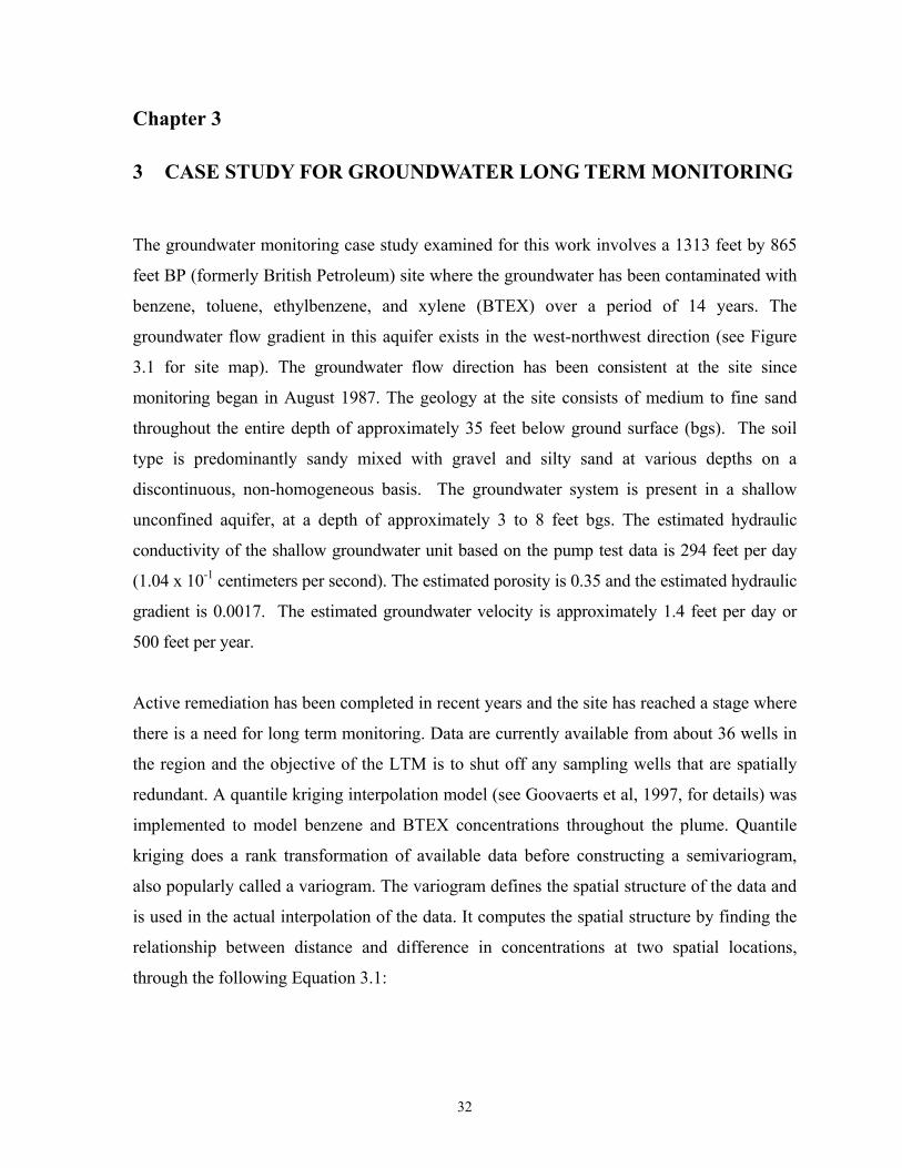
32
Chapter 3
3 CASE STUDY FOR GROUNDWATER LONG TERM MONITORING
The groundwater monitoring case study examined for this work involves a 1313 feet by 865
feet BP (formerly British Petroleum) site where the groundwater has been contaminated with
benzene, toluene, ethylbenzene, and xylene (BTEX) over a period of 14 years. The
groundwater flow gradient in this aquifer exists in the west-northwest direction (see Figure
3.1 for site map). The groundwater flow direction has been consistent at the site since
monitoring began in August 1987. The geology at the site consists of medium to fine sand
throughout the entire depth of approximately 35 feet below ground surface (bgs). The soil
type is predominantly sandy mixed with gravel and silty sand at various depths on a
discontinuous, non-homogeneous basis. The groundwater system is present in a shallow
unconfined aquifer, at a depth of approximately 3 to 8 feet bgs. The estimated hydraulic
conductivity of the shallow groundwater unit based on the pump test data is 294 feet per day
(1.04 x 10⁻¹ centimeters per second). The estimated porosity is 0.35 and the estimated hydraulic
gradient is 0.0017. The estimated groundwater velocity is approximately 1.4 feet per day or
500 feet per year.
Active remediation has been completed in recent years and the site has reached a stage where
there is a need for long term monitoring. Data are currently available from about 36 wells in
the region and the objective of the LTM is to shut off any sampling wells that are spatially
redundant. A quantile kriging interpolation model (see Goovaerts et al, 1997, for details) was
implemented to model benzene and BTEX concentrations throughout the plume. Quantile
kriging does a rank transformation of available data before constructing a semivariogram,
also popularly called a variogram. The variogram defines the spatial structure of the data and
is used in the actual interpolation of the data. It computes the spatial structure by finding the
relationship between distance and difference in concentrations at two spatial locations,
through the following Equation 3.1:

33
( ) ( )2)()(21 hxzxzh ii +−=γ (3.1)
Where, γ(h) is the experimental variogram value when two locations are a distance h apart,
z(xi) is the concentration at some location xi, and z(xi +h) is the concentration at some
location a distance h away. The experimental variogram values for all distances h versus h
are plotted and a theoretical curve is then fit through them. Figure 3.2, Figure 3.3, Figure 3.4,
and Figure 3.5 show the variograms of the transformed dataset, for the four contaminants.
Table 3.1 lists the various optimized parameters for the four variograms. Note that the data
points plotted in these graphs for the experimental variogram do not represent all possible
pairs of data points. Instead, they represent the binned values which consist of all point pairs
(h, γ(h)) that have similar h values. The median values of these point pairs are used in the
variogram to make the results resilient to outliers in the data. It can be observed that except
for Xylene, which mostly has a nugget structure in its variogram, other contaminants have
experimental variograms that can be fit to a spherical type variogram. It should also be noted
that the high nugget values of these variograms exist due to uncertainty in the estimation
because of a lack of enough closely spaced wells with small values of h. However, since the
decision maker (DM) would be more experienced with the history and geology of the site,
the Interactive Genetic Algorithm can assist the DM to include her/his knowledge about
spatial structure of the plumes through her/his preferences when she/he evaluates the quality
of the model predictions (see Chapters 4, 5, and 6 for the DM’s evaluation of the
interpolation model’s predictions). For the actual interpolation, ordinary kriging, which
assumes a locally constant but unknown mean, was used for this transformed data. Once
interpolation was completed, the estimated values were back transformed to the original form
of the data. In this case study, interpolation was done for all 4 constituents and the final
estimated values were summed to obtain the prediction for BTEX. Figure 3.6 shows the
interpolated maps of benzene and BTEX for all 36 monitoring wells.
Note that the selection of the quantile kriging model was based on an independent study
(Groves et al., 2004) performed for the BP’s LTM site by a collaborating team from Moire
Inc., Atlantic Richfield, Delta Environmental Consultants, Inc., and University of Illinois at
Urbana Champaign. They had compared different modeling methods, such as ordinary

34
kriging, quantile kriging, and inverse distance weighting, and then based on the performance
of jack-knifing errors found the optimized quantile kriging as the most appropriate
interpolation method. Jack-knifing is a method that evaluates performance of a model by
removing a single sample data point (i.e. monitoring well in this case) from the dataset and
then generating a model from the remaining samples. This model is used to find the error in
prediction at the site location where the data was withheld. This process is then repeated for
all other available sample data points. Figures 3.7 and Figure 3.8 show the jack-knifing errors
from the report submitted by Groves et al. (2004) for both benzene and BTEX, which were
used to determine the suitability of quantile kriging model over others. It can be seen that
quantile kriging had the lowest errors for the highest number of wells relative to the other
methods.
For this case study spatially redundant wells were identified through an LTM formulation
similar to Reed et al. (2001, 2004). The monitoring decision variables for the problem were
the sampling flags (xi = 0/1) for all 36 wells, where i varies from 1 to 36. Hence, if a flag is 1
then the well at the ith location is sampled. For example, the chromosome
“110000000100000000000000000000000011” indicates that the 1st, 2nd, 10th, 35th, and 36th
wells are all active monitoring wells, where as the others are all shut off. The numerical
objectives for this problem were to minimize the number of wells sampled (Equation 3.2)
and to minimize the maximum error between actual benzene concentrations and those
estimated with the benzene interpolation models using a subset of K wells (Equation 3.3).
The error in Equation 3.3 is normalized by a user-specified allowable error limit Eallow,Benzene.
Numerical Objective 1: ∑=
n
iixMinimize
1
, where
=otherwise
sampledisiwellifxi 0
1 (3.2)
Numerical Objective 2:
−
=Benzeneallow
esti
actuali
K E
KccErrorMaxMinimize
,
)(for Benzene (3.3)
Initial results for this application indicated that benzene is the major constituent of concern in
designing the monitoring system. To ensure that the overall BTEX concentration errors still

35
remain reasonable, a constraint was included to limit the BTEX error to a user-specified
allowable error limit Eallow,BTEX.
Constraint: 1)(
,
≤
−
=BTEXallow
esti
actuali
K E
KccErrorMax for BTEX (3.4)
The values for Eallow,Benzene and Eallow,BTEX were set to 5 ppb for benzene and 100 ppb for
BTEX, respectively, at this site. In addition to these objectives, two qualitative (or
subjective) criteria were considered in the IGA framework. The first criterion, which plays a
vital role in determining a good monitoring design, is how similar the overall contaminant
spatial distribution (i.e., the contaminant plume map) remains after the wells are removed
from the sampling plan. This is important to ensure no abnormal high concentrations are
detected near the boundaries that can cause contention between the site owners and
regulators. Accurate prediction of concentrations near the boundary is important to ensure
that the plume does not cross the site boundary onto public property. The second criterion is
how well defined the leading edge of the plume (the direction in which the groundwater is
flowing) remains (i.e., how low the local interpolation errors at the leading northwestern
boundary of the site are, after removing particular wells). In the IGA framework, when a real
decision maker is involved, the human will make these subjective judgments based on their
experience and visual perceptions of the plume maps. For the pseudo-human (i.e. the
simulated decision maker models) involved in this work, human preference are simulated by
including the local spatial errors at the leading edge boundaries (1100 feet by 100 feet north
boundary region) or at the central region of the plumes which have the main hotspots (i.e.
high concentration zones), into the fuzzy logic model and by setting decision rules for these
local errors. The subsequent chapters will discuss the details of constructing such simulated
decision makers using fuzzy logic modeling methods.

36
Table 3.1 Optimized variogram and kriging parameters for the four quantile-transformed contaminant datasets
Variogram Nugget
Spherical Variogram Coefficient
Spherical Variogram Range
Neighborhood Threshold Radius
Minimum Number of Neighbors
Maximum Number of Neighbors
Benzene 44.84 76.741 336.97 287.53 7 19 Toluene 40.60 129.24 1052.30 894.98 3 18 Ethylbenzene 70.25 23.03 1145.46 988.76 2 12 Xylene 124.96 9.57 1036.72 737.51 7.2 14
Pipeline Location
General Groundwater Flow Direction
Pipeline Location
General Groundwater Flow Direction
Figure 3.1 Current monitoring wells network at the BP site
Figure 3.2 Benzene variogram

37
Figure 3.3 Toluene variogram
Figure 3.4 EthylBenzene variogram
Figure 3.5 Xylene variogram

38
Figure 3.6 Plume maps for benzene and BTEX using all wells, concentration units in ppb
Benzene Jack-knifing Errors
-400
-300
-200
-100
0
100
200
1 10 9 27 29 14 3 8 31 36 17 33 11 2 16 20 32 19
Well IDs
Ben
zene
Err
ors
(ppb
)
Inverse Distance WeightingOrdinary KrigingQuantile Kriging
Figure 3.7 Benzene jack-knifing error model comparison for the BP site. The x-axis is sorted by the actual concentration (ppb) at each well. The lowest concentrations are generally more accurately predicted than the largest

39
BTEX Jack-knifing Errors
-1500
-1000
-500
0
500
1000
1500
20 1 27 29 8 36 13 24 25 15 21 28 19 9 4 31 6 5
Well IDs
BTE
X Er
rors
(ppb
)Inverse Distance WeightingOrdinary KrigingQuantile Kriging
Figure 3.8 BTEX jack-knifing error model comparison for the BP site. The x-axis is sorted by the actual concentration (ppb) at each well. The lowest concentrations are generally more accurately predicted than the largest

40
Chapter 4
4 STANDARD INTERACTIVE GENETIC ALGORITHM (SIGA): A
COMPREHENSIVE OPTIMIZATION FRAMEWORK FOR LONG-
TERM GROUNDWATER MONITORING DESIGN
This chapter begins by discussing the interpretation of optimal designs that also satisfy
subjective criteria, in the context of groundwater long-term monitoring optimization. It then
lays out the main objectives of this chapter, followed by the methodology section that
explains the design issues related to the SIGA search methodology when human fatigue is an
important influential factor. The results and discussion section compares the performance of
the different SIGA strategies and also compares the SIGA with a non-interactive genetic
algorithm. The final section is the conclusion section that reviews the advantages and
limitations of the SIGA framework.
4.1 Introduction
Henig and Buchanan (1996) describe a decision problem as comprising a set of objectively
defined alternatives and a set of subjectively defined criteria. The goal of a decision making
process should be to include both objective and subjective preferences of the decision maker
that help identify a comprehensive description of the world and expand the set of
alternatives. Subjective preferences arise from the decision maker’s (DM’s) sets of beliefs,
values, and knowledge built from experience and reasoning. However, purely subjective
judgements are prone to errors due to cognitive bias and wishful thinking. Also, Burrell and
Morgan (1979) have explained that the distinction between subjective and objective
interpretations of the world can give rise to fundamentally different views of the world,
which as a result affect the study of the world. Hence, the decision making process should
attempt to utilize subjective knowledge based on experience and reasoning as means to
complement the formal objective knowledge based on scientific and technical evidence.
However, it should also be noted at this point, that there are always certain aspects of the
problem that cannot be realized by using either objective or subjective reasoning, and in
those cases the beliefs or values of the DM assist in discriminating alternatives.

41
For example, Figure 4.1 shows various groundwater LTM designs in the space defined by the
formal objectives ‘Benzene Error’ and ‘Number of Wells’, as formulated in chapter 3 for
BP’s groundwater monitoring site at MI. These designs were obtained by compiling all the
populations over all the generations of a multiobjective Genetic Algorithm that was used to
optimize the LTM problem, on the basis of the formal objectives and constraints formulated
in Chapter 3. The multiobjective Genetic Algorithm (i.e. the NSGA II) evolved for 72
generations with a population size of 1000. Solutions near the bottom boundary of the
objective space are superior in quality than designs close to the top boundary that either have
worse formal objectives or violation of BTEX error constraint. If a numerical multiobjective
optimization algorithm (such as the NSGA II) was to be implemented for this problem based
on the two quantitative objectives and the constraint, the final pareto front would consist of
the designs marked by the filled black circles along the southernmost boundary. However,
the formal objectives, though based on scientific knowledge related to the problem, alone
cannot completely capture the extent of the true optimal space for the problem because of
reasons discussed earlier in chapter 1 and 2. When the DM’s subjective knowledge of the
problem is used to assist in identifying the extent of that true optimal space, solutions that are
seemingly slightly inferior to the final pareto front in the objective space defined by only the
formal objectives (as in Figure 4.1) can end up being included in a final set of optimal
alternatives that have promising formal objective and subjective evaluations. In addition,
though the subjective knowledge of the decision maker can help identify some portions of
that true optimal space, the conception of the subjectivity should honor the feedback from the
formal analysis. On the basis of the discussion initiated by Hagen and Buchanan (1996), it
can be deduced that in a well formulated multiobjective optimization problem, solutions (or,
alternatives/designs) in the formal objectives space can be separated into two categories: a)
Clearly inferior solutions that fail drastically in their formal evaluations (i.e. the quantitative
objectives and constraints) and have no potential to be selected for their subjective quality by
the DM, and b) Desirable solutions whose formal evaluations are acceptable or superior
from the decision maker’s perspective. It is this second region of desirable solutions that are
of most interest to the decision maker since their subjective evaluation will be complemented
by their performance in the formal evaluations. In practice, the boundaries between these

42
regions are usually not well defined and vary from problem to problem. However, the experts
can be the best judges at identifying these regions based on their expectations and goals.
From the perspective of the Interactive Genetic Algorithm system, it becomes crucial to
design the search process in such a way that a large number of alternatives, which lie in this
region of desirable solutions and respect the subjective criteria of the experts, are generated.
The Standard Interactive Genetic Algorithm (SIGA), which is designed to achieve such a
comprehensive search process, identifies diverse desirable solutions by interactively
including the subjective evaluations based on the DM’s preferences within its search
mechanism. For a multiobjective problem that has n formal objectives, the SIGA expresses
the subjective evaluation in the form of an additional n+1th objective (also called as the
Human Rank, as discussed in Chapter 2) to the problem. In previous Interactive Evolutionary
Computation setups (see Banzhaf (1997), Takagi (2001), Cho et al. (1998), Kamalian et al.
(2004) for examples), subjective evaluation has usually been adopted as a single objective in
the form of a rank or score within the optimization process. However, the SIGA framework
used in this research uses a multiobjective scheme to consider the importance of formal
objectives that are also essential for defining the true optimal design space of engineering
applications.
In context of the above, the main objectives of this chapter are to:
1. Explore strategies for effectively designing a SIGA framework that uses a single
interacting expert. The two important aspects of the design that are investigated are:
a) sizing of populations for SIGA to control human fatigue, and b) identification of
effective starting populations that can help determine solutions in the desirable region
when small population sizes are used for SIGA.
2. Compare SIGA with Non-Interactive Genetic Algorithm (NGA) for their
effectiveness in identifying robust solutions that satisfy the DM’s subjective criteria.
4.2 Methodology
This section initially investigates different empirical guidelines for sizing populations and
other genetic algorithm parameters for the SIGA. Different methodologies are then proposed

43
for initiating the starting populations of the SIGA to improve the capability of the SIGA to
identify diverse desirable solutions that have superior subjective evaluation. To allow
rigorous testing with consistent criteria, these starting strategies will be tested using a
simulated decision maker that emulates the human decision maker’s criteria and nature of
preferences. Hence, the last sub-section will discuss the design of this simulated decision
maker.
4.2.1 Population Sizing and Other Genetic Algorithm Parameters for SIGA
The SIGA is designed to interact with the human (i.e., the expert or decision maker) during
every generation of the GA process. The expert evaluates the overall suitability (‘subjective
fitness’) of candidate solutions (see Chapter 2 and Figure 1.2 for more details) and assigns a
Human Rank value to the n+1th objective for the population. The other n objectives and/or
any quantitative constraints are evaluated using formal models/equations. The GA then
performs the usual operations of selection, crossover, and mutation to create new solutions
by analyzing these n+1 objectives. The search mechanism of the SIGA, described in this
research, is based on the Non-Dominated Sorted Genetic Algorithm II (NSGA II, Deb et al.,
2000).
Since the human is involved in analyzing populations of solutions over many generations,
human fatigue becomes an important factor that affects the design of SIGA framework. As
discussed in Chapter 2, most existing Interactive Genetic Algorithm (IGA) frameworks
usually use small populations to control the human fatigue. However, usage of small
populations can impair the performance of the genetic algorithm search. In this section, the
following guidelines are listed to help practitioners appropriately determine lower bounds on
population sizes for a small population IGA.
1) Reed et al (2003): Their work on sizing populations for multiobjective GAs can be used
as a rule of thumb to obtain a lower bound on the population size. They propose that N >
2* Rnd, where N is the population size and Rnd is the number of desirable non-dominated
solutions on the Pareto front. For the LTM problem described in Chapter 3, Rnd was
chosen to be 12 (i.e. designs that have number of wells varying from 20 to 31, since
designs with number of wells < 20 violate the BTEX constraint and those with number of
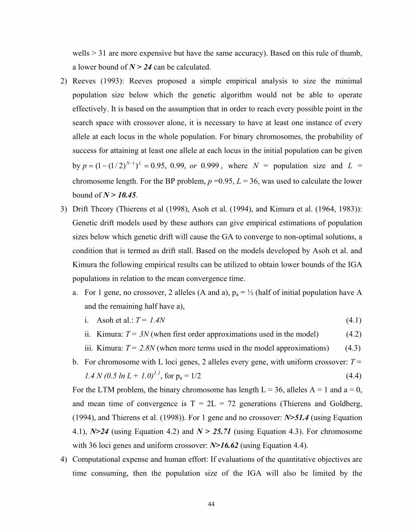
44
wells > 31 are more expensive but have the same accuracy). Based on this rule of thumb,
a lower bound of N > 24 can be calculated.
2) Reeves (1993): Reeves proposed a simple empirical analysis to size the minimal
population size below which the genetic algorithm would not be able to operate
effectively. It is based on the assumption that in order to reach every possible point in the
search space with crossover alone, it is necessary to have at least one instance of every
allele at each locus in the whole population. For binary chromosomes, the probability of
success for attaining at least one allele at each locus in the initial population can be given
by 999.0,99.0,95.0))2/1(1( 1 orp LN =−= − , where N = population size and L =
chromosome length. For the BP problem, p =0.95, L = 36, was used to calculate the lower
bound of N > 10.45.
3) Drift Theory (Thierens et al (1998), Asoh et al. (1994), and Kimura et al. (1964, 1983)):
Genetic drift models used by these authors can give empirical estimations of population
sizes below which genetic drift will cause the GA to converge to non-optimal solutions, a
condition that is termed as drift stall. Based on the models developed by Asoh et al. and
Kimura the following empirical results can be utilized to obtain lower bounds of the IGA
populations in relation to the mean convergence time.
a. For 1 gene, no crossover, 2 alleles (A and a), pa = ½ (half of initial population have A
and the remaining half have a),
i. Asoh et al.: T = 1.4N (4.1)
ii. Kimura: T = 3N (when first order approximations used in the model) (4.2)
iii. Kimura: T = 2.8N (when more terms used in the model approximations) (4.3)
b. For chromosome with L loci genes, 2 alleles every gene, with uniform crossover: T =
1.4 N (0.5 ln L + 1.0)1.1, for pa = 1/2 (4.4)
For the LTM problem, the binary chromosome has length L = 36, alleles A = 1 and a = 0,
and mean time of convergence is T = 2L = 72 generations (Thierens and Goldberg,
(1994), and Thierens et al. (1998)). For 1 gene and no crossover: N>51.4 (using Equation
4.1), N>24 (using Equation 4.2) and N > 25.71 (using Equation 4.3). For chromosome
with 36 loci genes and uniform crossover: N>16.62 (using Equation 4.4).
4) Computational expense and human effort: If evaluations of the quantitative objectives are
time consuming, then the population size of the IGA will also be limited by the

45
computational costs and resources (i.e. the type of single or parallel computing
infrastructure available). The amount of available time for human interaction with the
machine will also limit this population size. In our work, we use the empirical analysis
(discussed above) along with the computational and human labor limitations to decide the
population size for IGA frameworks.
Based on the above empirical results and expected amount of manageable human labor, a
small population size of 30 was selected for all IGAs implemented on the LTM problem.
Crossover (i.e. Uniform Crossover) and mutation rates of 0.75 and 0.03 were used
respectively based on recommendations by Reed et al. (2003). Tournament selection without
replacement (tournament size 2) was used for selecting the mates for crossover.
4.2.2 Starting Strategies for SIGA
Providing a good starting population to the SIGA algorithm is essential for supplying good
building blocks which ensures better solutions are found. Moreover, from the expert’s
perspective, having an initial set of good solutions at the beginning of interaction helps
her/him to avoid unnecessary wasting of cognitive effort in learning about the problem and
her/his personal preferences.
Four different starting strategies were explored for small population SIGAs:
1) Random starting strategy (“Random”): All individuals in the starting population of the
SIGA are randomly created. The quality of the starting population thus depends on the
random number seed.
2) Pre-optimized large population starting strategy (“Large”): A large population GA is first
evolved for a few generations based only on the quantitative objectives. When the expert
agrees that initial exploration has reached her/his notion of the ‘region of desirable
solutions’ in quantitative objective space, the initial search is stopped and the SIGA
begin. The starting population of the small population SIGA is then selected from this
pre-optimized large population. For the LTM problem, a population size of 1000 was
evolved on the quantitative objectives for 24 generations to create 11 distinct optimal
solutions that were fed into SIGA’s starting populations. Though this approach can

46
provide good starting designs for the SIGA from a well searched solution space, the
major drawback of this approach is the large number of fitness evaluations required for
the large population. For applications where fitness function evaluation is very
computationally intensive, this approach can be expensive. Even for the case study
currently being explored, which is otherwise not a very computationally expensive
problem compared to many other water resources applications, it took approximately 20
hours to complete a GA run for population size 1000 and 24 generations on a desktop
with 2.8 GHz Pentium 4 processor and 512 MB RAM.
3) Composite pre-optimized small populations of different sizes (“Composite_diff”): Small
populations of different sizes are first optimized nominally for a couple of generations
and then combined to form a composite population. The starting population of the small
population SIGA is then sampled from this pre-optimized composite population. To
create the composite population for LTM problem, the initial search on quantitative
objectives was done by using 5 populations of size 10, 20, 30, 40, and 50 for 24
generations. The final populations of these 5 experiments were then combined to create a
composite population of 14 solutions, which were then fed into the initial populations of
SIGA. The strength of this strategy lies in its much lower computational effort than the
strategy 2 above. Also, by allowing an initial exploration using different sizes of small
populations, the strategy has the advantage of using different selection pressures
(dependent on population sizes) for collecting good building blocks within the
chromosomes.
4) Composite pre-optimized small populations of same size (“Composite_Same”): This
strategy is similar to the previous strategy, except that the composite population is created
by doing initial exploration on small populations of the same size (same selection
pressures) but different random number seeds. For the LTM problem population sizes of
30 for 5 different random seeds were searched on quantitative objectives to produce 13
distinct solutions that were combined to create the composite population. Use of different
random number seeds ensures that the effect of an unfortunate random number seed does
not bias the quality of the solutions in the composite population. And, like the previous
strategy, the strength of this strategy also lies in its low computational effort.

47
4.2.3 Design of Simulated Decision Maker
When expert interaction is allowed to affect the optimization process, the interacting expert’s
attention span, focus, preferences and other cognitive attributes can vary over time. This kind
of disturbance manifests itself as noise in the subjective feedback and is difficult to remove
completely from the system. To avoid this issue in this work and enable rigorous comparison
of the starting strategies for SIGA, the effect of this environmental interference will be
temporarily eliminated by creating automated simulated decision makers (also referred to as
pseudo-humans). The pseudo-human is like an expert in the perfect world, who only gets
affected by the internal state of her/his mind and not by external uncertainties of the world. In
this work, the pseudo-human was created using fuzzy set theory. Fuzzy set theory was
implemented to represent the human’s decision making process because, as discussed earlier
in chapter 3, it has been successfully used in the past to express the vagueness and
approximate reasoning of human expression. Also, Jones (1977) claims that the human brain
uses fuzzy concepts, fuzzy measurements of inputs and makes fuzzy logical inferences while
processing information. There are many other machine learning methods that could also be
explored to simulate expert preferences, but that will be left as a topic to be explored for
future research.
The fuzzy pseudo-human was created using five decision making criteria, related to the
monitoring designs, as fuzzy inputs to a mamdani style fuzzy logic model. The inputs
selected for this pseudo-human are benzene error (Equation 3.2 in Chapter 3), number of
wells (Equation 3.1 in Chapter 3), BTEX error constraint violation (Equation 3.3 in Chapter
3), local benzene error in the northern boundary region, and local BTEX error in the northern
boundary region. To calculate the local benzene and local BTEX errors, for every LTM
design, contaminant concentrations are predicted at 150 random locations in a northern
boundary region (1100 ft by 100 ft), and means of absolute errors in contaminant predictions
are evaluated at all these locations for the LTM design in comparison to the solution that has
all 36 wells being monitored. The output of the model is the fuzzy sets for Human Ranks.
Figure 4.2 shows the trapezoidal membership functions for the fuzzy inputs and the output
(i.e. the Human Rank) for this pseudo-human. The membership functions and rules were set
by the author in order to create a pseudo-human that would prefer designs in the desirable

48
region (refer to Figure 4.1) and would rank most solutions in the clearly inferior region as
below average. The Human Ranks in this work vary from 1 to 5; where 1 stands for “best,” 2
stands for “good,” 3 stands for “average,” 4 stands for “bad,” and 5 stands for “worst”.
Different rules were also created for this fuzzy pseudo-human to simulate the psychology of
the expert. The 48 rules created for this pseudo-human cover all possible combinations of
fuzzy inputs, and are attached in the appendix A (Table A.1). The rules were created
assuming that the decision maker’s main goal is to find solutions that perform well with
respect to both the formal criteria and the subjective criteria. Such solutions would be
classified as above-average designs from her/his perspective. For example in Table A.1, Rule
10 “if benzeneError is good and numberOfWells is bad and btexError is good and
localBenzeneError is good and localBtexError is bad then humanRank is good” is based on
the logic that “good” quality of the different error estimations in the predictions of various
contaminants would be preferred by the decision maker. Hence, such designs would be
assigned an above-average Human Rank, even if the number of wells are “bad” (i.e.
expensive monitoring plans). It can also be assumed from the previous discussion (Section
4.1) that most designs in the desirable region of the objective space, that also satisfy the
subjective criteria, would be deemed as above-average by the decision maker. Figure 4.3
shows that the pseudo Human Ranks produced by the above fuzzy logic model honor such a
trend where most solutions in the desirable region are above-average (i.e. pseudo Human
Rank < 3) and solutions in the significantly inferior region of the objective space of formal
objectives have below-average ranks (i.e. pseudo Human Rank ≥ 3). The need to create a
pseudo-human in this manner is motivated by the discussion in the introduction section of
this chapter, where it was realized that when subjective preferences are considered along with
the formal objectives then solutions seemingly slightly sub-optimal in their formal objectives
can actually have better overall quality and thus superior Human Ranks.
4.3 Results and Discussion
The first sub-section below presents results related to the effect of the starting strategies on
the performance of the interactive search. As discussed before, for testing purposes pseudo
humans will be used in this section. The second sub-section uses the best starting strategy for
the SIGA and compares the performance of the SIGA (by using real humans) and the Non-

49
Interactive Genetic Algorithm (NGA) in their ability to find promising solutions that meet
the expert’s subjective criteria.
4.3.1 Comparison of Starting Strategies by Using Pseudo-Human
Figures 4.4 and 4.5 show results for the four different starting population strategies explored
for the SIGA. Since genetic algorithms use probabilistic operators for selection, crossover
and mutation mechanisms, 25 experiments with different random number seeds were
performed for each of these strategies. All 25 experiments, however, had identical settings
for GA parameters and operators (for example, population size = 30, number of generations
= 72, etc.). The main aim of these experiments is to identify starting strategies that yield the
greatest number of above-average solutions in the region of desirable solutions (shown in
Figure 4.3) when the human’s subjective criteria is added as an additional objective.
For the tradeoffs in Figures 4.4 and 4.5, except for the random starting strategy (‘Random’),
most of the solutions (obtained from 25 experiments for 25 different random number seeds)
obtained via the non-random starting strategies are concentrated in the lower edge of the
region of desirable solutions. In other words, most of these solutions have lower benzene
errors and lower Human Ranks, which indicate better quantitative and qualitative
characteristics for these solutions respectively. Hence, it is clear that when small populations
are used for SIGA, an initial injection of competent building blocks into the starting
populations is more robust in finding diverse high performance solutions, than merely
starting the SIGA using a randomly selected population.
Two one-tailed nonparametric tests, the Sign test (p<0.05) and the Wilcoxon Matched-Pairs
Signed-Ranks test (p<0.01), were done on the results obtained for all four strategies to
compare their ability to find above-average solutions. See Siegel et al. (1988) for details on
these two methods. Table 1 reports the number of above-average solutions found by each
strategy, for each of the 25 experiments. It is important to note here that each experiment
used a particular random number seed that was common for all the four strategies for that
experiment. Table 2 compares the results of the experiments tabulated in Table 1. One can
observe that both tests indicate that the pre-optimized large population starting strategy
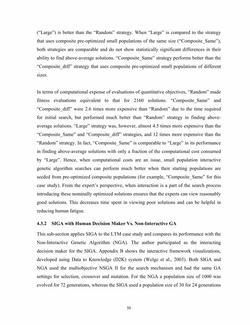
50
(“Large”) is better than the “Random” strategy. When “Large” is compared to the strategy
that uses composite pre-optimized small populations of the same size (“Composite_Same”),
both strategies are comparable and do not show statistically significant differences in their
ability to find above-average solutions. “Composite_Same” strategy performs better than the
“Composite_diff” strategy that uses composite pre-optimized small populations of different
sizes.
In terms of computational expense of evaluations of quantitative objectives, “Random” made
fitness evaluations equivalent to that for 2160 solutions. “Composite_Same” and
“Composite_diff” were 2.6 times more expensive than “Random” due to the time required
for initial search, but performed much better than “Random” strategy in finding above-
average solutions. “Large” strategy was, however, almost 4.5 times more expensive than the
“Composite_Same” and “Composite_diff” strategies, and 12 times more expensive than the
“Random” strategy. In fact, “Composite_Same” is comparable to “Large” in its performance
in finding above-average solutions with only a fraction of the computational cost consumed
by “Large”. Hence, when computational costs are an issue, small population interactive
genetic algorithm searches can perform much better when their starting populations are
seeded from pre-optimized composite populations (for example, “Composite_Same” for this
case study). From the expert’s perspective, when interaction is a part of the search process
introducing these nominally optimized solutions ensures that the experts can view reasonably
good solutions. This decreases time spent in viewing poor solutions and can be helpful in
reducing human fatigue.
4.3.2 SIGA with Human Decision Maker Vs. Non-Interactive GA
This sub-section applies SIGA to the LTM case study and compares its performance with the
Non-Interactive Genetic Algorithm (NGA). The author participated as the interacting
decision maker for the SIGA. Appendix B shows the interactive framework visualizations,
developed using Data to Knowledge (D2K) system (Welge et al., 2003). Both SIGA and
NGA used the multiobjective NSGA II for the search mechanism and had the same GA
settings for selection, crossover and mutation. For the NGA a population size of 1000 was
evolved for 72 generations, whereas the SIGA used a population size of 30 for 24 generations

51
to contain human fatigue and effort. The starting population of NGA was random, whereas
the initial population of SIGA was created by using the “Composite_Same” strategy explored
earlier. For the SIGA, the solutions were qualitatively analyzed not only for their actual
objective values, but also to ensure that the interpolation of the plume had low errors near the
north and northwest boundaries of the site. It was also decided to make certain that spatial
structures of both benzene and BTEX plumes were also assessed qualitatively to ensure that
they were as similar to the ‘All Wells’ solutions (Figure 4.7) as possible. This was achieved
by comparing all the spatial zones with high concentrations (“hot spots”) and low
concentrations (“low spots”) of the contaminants for their delineation quality.
Figure 4.6 compares the tradeoff curves of the final population for the interactive and non-
interactive methodologies. Notice that the NGA (which uses a larger population size of 1000)
generally gives a better quantitative tradeoff curve with respect to benzene error and number
of wells as compared to the SIGA (which uses a small population size of 30). However, when
the Human Ranks are compared for these solutions, it is interesting to observe that many
solutions (when numbers of wells are 25, 26, 27, 28, 29, and 30) found by SIGA have equal
or better subjective quality than those found by NGA for the same number of wells, even
though these SIGA solutions have slightly worse benzene errors. Hence, this provides futher
evidence to the earlier assumption that in real world problems, many seemingly sub-optimal
solutions (from the perspective of quantitative objectives and constraints) exist in the region
of desirable solutions that can actually satisfy the subjective criteria better.
The actual solutions for NGA and SIGA were then compared to see how the human decision
maker’s interaction made a difference in the final solution set. Figures 4.8, 4.9, and 4.10
show interpolated plumes for the 27, 28, and 29 wells solutions respectively. When these
solutions are compared to the “All Wells” solution in Figure 4.7, it can be assessed that the
SIGA found solutions that respect the qualitative characteristics of the LTM problem much
better than their counterparts found by NGA. From the expert’s perspective, even though the
SIGA solutions have slightly worse benzene error, the subjective quality of the SIGA
solutions plays a major role determining the overall quality of the solution. The benzene and
BTEX plume delineations predicted by all 36 wells, in Figure 4.7, show that high

52
concentration zones (i.e. "hot spots") are well within the boundary traced by the outermost
wells. Also, though the groundwater flows in the northwest direction, these predictions show
no leakage of high concentrations across the boundary in any direction. The 27, 28, and 29
wells solutions proposed by SIGA and NGA respect the plume delineation of benzene within
the boundary, similar to the "All Wells" solution. However, the BTEX plume delineations are
not similar, even though the BTEX constraint (Equation 3.3) was satisfied for all these
solutions. For all the designs (Figures 4.8, 4.9, and 4.10), the solution proposed by SIGA has
better integrity in the containment of BTEX hot spots within the boundary, than the solutions
proposed by NGA. Also, for the 29-wells solution (Figure 4.10) proposed by SIGA, the
BTEX plume has a better similarity in shape to the 36 wells solutions (Figure 4.7) than the
29-wells solutions proposed by NGA. These results also divulge that the quantitative BTEX
constraint selected for the optimization process is not effective in ensuring search for
solutions that don’t have such qualitative anomalies in the spatial locations of hot spots.
These anomalies are, however, easily identified when the actual decision maker is involved
in the search process. The expert knows that at the site erroneous high and low valued
contaminant predictions in large/medium scale regions, respectively, can misrepresent the
suitability of the designs. Hence, the expert will favor those designs that not only perform
well in their formal analysis but also exhibit realistic predictions of the contaminants at the
site.
4.4 Conclusions
In this chapter, methodologies for designing a multi-objective Standard Interactive Genetic
Algorithm were explored. The salient findings of these investigations are:
• This study exhibits the need for a paradigm shift in optimization methods. By
including experts in the search processes when numerical representations of
objectives, constraints, etc. cannot completely define the problem specifics, it is
possible to incorporate useful knowledge that can help improve the overall suitability
of designs. For example, the interactive procedure implemented on the LTM problem
found solutions that respected the subjective criteria for plume delineation and the
concentration predictions near the boundary much better than the solutions found by
the non-interactive Genetic Algorithm. From the DM’s perspective, if the site owners

53
are willing to incur monitoring costs for up to 29 wells, then all three designs
proposed by SIGA (see Figure 4.8, 4.9, and 4.10) for 27, 28, and 29 wells would be
categorized as possible robust designs. This would allow the DM to save on
monitoring costs and still be in a position to propose cheaper well designs (e.g., 27
and 28 monitoring wells) that meet the objectives of the interested parties.
• In SIGA, the author handles the issue of human fatigue by decreasing population size
of the genetic algorithm. Many other researchers like Takagi (2001), Cho et al.
(1998), Kamalian et al. (2004) have used a similar approach. Though this work
investigated methods to help practitioners improve the performance of SIGAs that use
small populations (via systematic determination of an effective minimal population
size and starting strategies), there are other techniques that could also be explored for
controlling human fatigue. One approach involves using a combination of surrogate
models and human decision makers to allow the use of larger population IGAs while
keeping the effort of the human within a practical limit. Work also needs to be done
for handling other human factors (such as the human cognitive learning process,
nonstationarity in preferences, etc.) that have a considerable affect on the search
processes and is not currently handled by standard IGA frameworks. The next two
chapters explore the development of frameworks to address these issues.

54
Table 4.1 Number of above-average solutions found by different strategies
Experiment Random Starting Large
Composite-Same
Composite-diff
1 0 8 8 82 7 9 10 83 0 10 8 84 5 8 9 75 6 8 8 86 0 9 8 77 0 9 10 88 0 8 7 79 5 8 7 7
10 0 8 10 711 9 9 7 712 10 9 8 713 5 8 6 814 8 9 7 615 6 8 9 816 1 7 10 717 0 7 9 718 7 8 7 619 0 8 7 620 0 8 9 821 2 8 10 722 0 8 9 723 0 8 8 924 8 8 9 825 7 7 10 7
Table 4.2 Best SIGA starting strategies when compared via Sign test and Wilcoxon Matched-Pairs Signed-Ranks test
Strategies comparison Sign Test (p<0.05) Wilcoxon Matched-Pairs Signed-Ranks
Test (p<0.01) Random Vs. Large: Large is better Large is better
Large Vs. Composite_Same: Either Either
Composite_Same Vs. Composite_diff:
Composite_Same is better Composite_Same is better

55
0
20
40
60
80
100
120
140
160
180
10 15 20 25 30 35 40
Number of Wells
Ben
zene
Err
or
Clearly Inferior Solutions: Does the human need to inspect these?
Region of desirable solutions0
20
40
60
80
100
120
140
160
180
10 15 20 25 30 35 40
Number of Wells
Ben
zene
Err
or
Clearly Inferior Solutions: Does the human need to inspect these?
Region of desirable solutions
Figure 4.1 Various long-term monitoring designs for BP’s site at MI, based only on the formal quantitative objectives ‘Benzene Error’ and ‘Number of Wells’, and formal quantitative constraint for BTEX Error
Figure 4.2 Membership functions of fuzzy pseudo human

56
1
1.5
2
2.5
3
3.5
4
4.5
10 15 20 25 30 35
Number of Wells
Pseu
do H
uman
Ran
k
Region of desirable solutions
Inferior Solutions
1
1.5
2
2.5
3
3.5
4
4.5
10 15 20 25 30 35
Number of Wells
Pseu
do H
uman
Ran
k
Region of desirable solutions
Inferior Solutions
Figure 4.3 Pseudo Human Ranks for the designs in the space of quantitative objectives
0
10
20
30
40
50
60
70
18 20 22 24 26 28 30 32 34 36
Number of Wells
Ben
zene
Err
or
RandomLargeComposite_SameComposite_diff
Figure 4.4 Benzene error and number of wells tradeoff: Effect of starting strategies on SIGA, for all 25 experiments

57
1
1.5
2
2.5
3
3.5
4
18 23 28 33
Number of Wells
Pseu
do H
uman
Ran
kRandomLargeComposite_SameComposite_diff
Figure 4.5 Pseudo Human Ranks and number of wells tradeoff: Effect of starting strategies on SIGA for all 25 experiments
0
20
40
60
80
100
120
20 25 30 35
Number of Wells
Ben
zene
Err
or (p
pb)
NGA
SIGA
0
1
2
3
4
5
6
20 22 24 26 28 30 32 34 36
Number of Wells
Hum
an R
ank
NGA
SIGA
Figure 4.6 Non-interactive Genetic Algorithm vs. Standard Interactive Genetic Algorithm
Figure 4.7 “All Wells” Solutions: Kriged maps for Benzene and BTEX plumes when all 36 wells are installed, concentration units in ppb

58
Benzene (ppb) BTEX (ppb) SIGA Human Rank 2
NGA Human Rank 3
Figure 4.8 27-well solutions found by SIGA and NGA. “o” are locations with active monitoring wells, “+” are locations with monitoring wells shut off.
Benzene (ppb) BTEX (ppb) SIGA Human Rank 1
NGA Human Rank 3
Figure 4.9 28-well solutions found by SIGA and NGA. “o” are locations with active monitoring wells, “+” are locations with monitoring wells shut off.
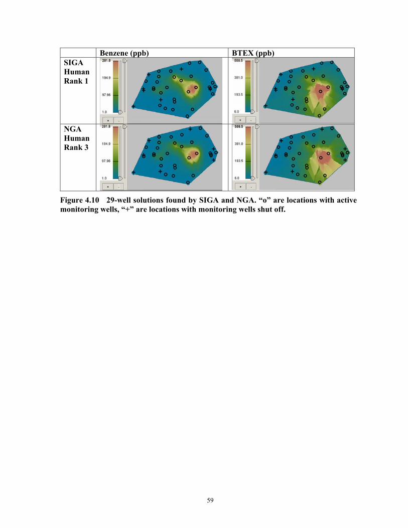
59
Benzene (ppb) BTEX (ppb) SIGA Human Rank 1
NGA Human Rank 3
Figure 4.10 29-well solutions found by SIGA and NGA. “o” are locations with active monitoring wells, “+” are locations with monitoring wells shut off.

60
Chapter 5
5 CASE-BASED MICRO INTERACTIVE GENETIC ALGORITHM
(CBMIGA) – AN ENHANCED INTERACTIVE OPTIMIZATION
FRAMEWORK FOR ADAPTIVE DECISION MAKING
The previous chapter discussed the benefits of using an interactive genetic algorithm over a
non-interactive genetic algorithm to search for promising solutions that perform well on both
formal (quantitative) and subjective criteria. It also investigated approaches to effectively
design the Standard Interactive Genetic Algorithm (SIGA) when human fatigue poses
constraints on the proficiency of the genetic algorithm’s search. This chapter investigates the
effect of the decision maker’s learning process on the interactive search process. It begins by
discussing the nature of human learning and the current limitations in SIGA’s ability to
accommodate for the learning process. The methodology section proposes a new framework,
Case-based Micro Interactive Genetic Algorithm (CBMIGA), which adapts to the decision
maker’s learning process and assists in searching for diverse solutions when the cognitive
learning process alters her/his perception of subjective preferences . Design issues related to
the CBMIGA search methodology are also discussed in this section, along with the design of
a simulated decision maker which is used for testing purposes. The results and discussion
section investigates the performance of the CBMIGA’s different design strategies using a
simulated decision maker, and then compares the CBMIGA with the SIGA and the non-
interactive genetic algorithm when a real decision maker is used for interaction. The final
section is the conclusion section that reviews the main findings of this chapter.
5.1 Introduction
When subjective analysis through interaction is a part of the search process, an efficient
search algorithm (the Genetic Algorithm in this case) should be able to:
1) Improve solution quality, with decreased dependence on the algorithm’s operators
and with tractable computational and human fatigue.

61
2) Use knowledge of previously found solutions to supply building blocks for new
solutions, especially when there are constraints on the number of computational
evaluations.
3) Adaptable to nonstationarity or changes in the fitness space that occur because of the
human’s learning process.
4) Cater to human error and environmental noise corrections.
5) Improve solution diversity across the Pareto front and in promising neighborhoods
(i.e., solutions with slightly inferior formal objectives, but superior subjective
evaluation).
The SIGA framework, explored in chapter 4, controlled human fatigue by limiting population
sizes. The knowledge of previously found solutions that performed well based on formal
criteria (i.e. the quantitative objectives and constraints) was utilized to provide good starting
points for the small population SIGA. This also provided the human with an initial pool of
reasonable solutions to form their opinions on subjective preferences without initially
searching randomly through many poor designs, thereby also limiting boredom and fatigue.
However, the SIGA framework did not fully address the effect of the decision maker’s
learning process in its design. The SIGA also did not provide any systematic framework to
facilitate the learning process when real decision makers participate. In the context of
solution diversity, the Pareto front in the final population was constrained to only those
solutions that survived the selection. Slightly suboptimal solutions were lost from the SIGA’s
population, irrespective of the superior Human Ranks. These lost solutions were not able to
influence future generations of the genetic algorithm which, as observed later in this chapter,
can be disadvantageous for the interactive search process. This chapter proposes a new IGA
framework – CBMIGA – to overcome these limitations. Before the details of the CBMIGA
framework are explained, the following subsection discusses the nature of human learning,
and its significance and effect on the design and functioning of any interactive genetic
algorithm framework.
62
5.1.1 Human Learning and the Interactive Genetic Algorithm
Recall from chapter 2 that learning in an interactive system is a process that helps decision
makers to construct their own knowledge of a system based on their experiences and
mistakes, whether from prior knowledge or knowledge gained during the interactive process.
During this process decision makers can alter their reasoning methods as they spend more
time analyzing the problem, and re-evaluating their reasoning and its consequences. Chi and
Glaser (1980) found that, unlike novices, experts use their learning process to construct
flexible reasoning strategies which, in turn, help them address problems in a more planned
manner. Experts also spend time understanding the features of the problem before attempting
to solve it. This introspective monitoring and continual correction of reasoning methods help
humans to manage the various complexities of problem-solving and decision making (Fox,
1995).
The interactive genetic algorithm provides an environment where the decision maker is likely
to go through this introspection and learning process as she/he compares designs and assigns
qualitative ranks to them. In the context of the multi-objective Interactive Genetic Algorithm
the qualitative objective function value (i.e. the Human Ranks) assigned to many solutions
would be susceptible to temporal changes as more knowledge is gained through the
interactions. These changes can be attributed to corrections of errors or due to nonstationarity
in preferences when the human’s reasoning strategy changes as solutions are evaluated.
Using such a time dependant objective function makes the genetic algorithm search process
susceptible to disruptions, if the framework is not designed to handle nonstationarity. This
situation can not only mislead the genetic algorithm to false optima, but it can also reduce
diversity in the genetic algorithm population when solutions that have worse numerical
values of objectives at an instance in time are not able to survive the GA’s selection process.
The CBMIGA proposed below is designed to handle such nonstationarity in objective
functions and preserve diversity of solutions, while providing a flexible learning environment
for the introspective decision maker.

63
5.2 Methodology
This section shall first discuss the design of the CBMIGA framework in detail, followed by a
description of the design of the simulated experts used in this chapter for testing the
performance of CBMIGA.
5.2.1 Design of the Case-based Micro Interactive Genetic Algorithm (CBMIGA).
The CBMIGA has two main components in its structure (Figure 5.1): Case-based Memory
(CBM) and Micro Interactive Genetic Algorithm (micro-IGA). Below is a step by step
explanation of the functioning of this framework.
Step 1. The CBMIGA algorithm starts by first creating the CBM, which is a reservoir of
previously found good solutions that can supply the genetic algorithm with building blocks
of desirable attributes in designs. This could either be an empty set or it could have an initial
collection of solutions from nominally pre-optimized populations. This reservoir of designs
gets continually furnished with solutions as the CBMIGA progresses. In this framework, the
starting strategy that creates a composite population from pre-optimized small populations of
same size (also called “Composite_Same”) is used to create the collection of initial CBM
solutions. Refer to Section 4.2.2 in Chapter 4 for more details on this strategy.
The proposed use of a CBM is influenced by the concept of case-based reasoning (Riesbeck
et al. (1989), Leake et al. (1996)), which reuses solutions of existing/previous problems to
solve a new problem. In this manner, case-based reasoning also provides an approach for
incremental and persistent learning. This kind of reasoning has been favorably used in
evolutionary search algorithms before by various researchers to introduce long-term elitism
and overcome various limitations of the genetic algorithm designs. Eggermont et al. (2001)
and Ramsey et al. (1993) successfully used case-based memories for non-stationary
evolutionary search where the fitness function landscape changed as the generations
progressed. Rasheed et al. (1997) used the case based approach within the GA for aircraft
design and missile inlet design. They observed that usage of CBM not only improved the
reliability of their genetic algorithm (GA), it also made the GA less sensitive to poor choices
of parameter values (e.g. mutation rate, etc.). Louis et al. (2004) proposed the Case Injected

64
Genetic AlgoRithm (CIGAR) that would inject GA populations with appropriate solutions as
the search progressed. In their applications for combinational circuit design, strike force asset
allocation and job shop scheduling, they also observed an improvement in both solution
quality and computational efficiency of the search. Usage of the CBM within the Interactive
Genetic Algorithm framework will not only help in dealing with the nonstationarity in the
Human Ranks objective, it will also help overcome the limitations in search capability of
small population IGAs by utilizing the building block information stored within the CBM
solutions. By saving the newly created solutions with superior Human Ranks in the CBM,
their building block information will be continually used to create new diverse solutions.
Step 2. Once this initial CBM pool is created, the expert is invited to rank these solutions and
acquaint herself/himself with their design characteristics. Once this initial introspection is
over, the next step involves preparing a micro-IGA for active search (see Figure 5.1).
Micro-IGAs are small population Interactive Genetic Algorithms that have a periodic
reinitialization of the population after a few generations of search. Their non-interactive
counterpart, known as the Micro Genetic Algorithm (micro-GA), was originally suggested by
Goldberg (1989), and has been widely used by researchers to improve efficiencies of small
population GAs and nonstationary problems (e.g., Coello et al. (2000), Krishnakumar (1989),
Grefenstette (1992)). The reinitialization process of the micro-GAs allows continuous
introduction of diversity in the population to allow the GA to effectively respond to changing
fitness space or search through vast complex fitness space, despite small population sizes.
Various population sizes have been used by researchers within the micro-GAs, from values
as low as 4 (Coello et al. (2000)) to as high as 100 (Grefenstette (1992)). From the Interactive
Genetic Algorithm perspective, micro-IGAs can be beneficial in a) improving search
performance with decreased computational and human effort, b) introducing diversity in the
converging population without allowing the selection mechanism, which makes copies of the
best chromosomes, diminish the diversity of the population with a fixed size, and c) helping
the IGA effectively restart the search process without getting trapped in a particular region of
decision space (especially when the nonstationarity in human preferences introduces
temporal modifications in the structure of the Human Ranks objective space).

65
Step 3. This step involves creating the starting population of the micro-IGA, which consists
of (x) % solutions obtained from the CBM and (100-x) % generated randomly to improve
diversity and exploration. Retrieval of solutions from the CBM can be done randomly or
non-randomly. Non random methods can either retrieve the best solutions from CBM or use
heuristic methods such as prediction algorithms (Eggermont et al. (2001)) and similarity
metrics (Louis et al. (2004)), etc. Such heuristic methods require knowledge of the problem
space or solution space and their determination can be non-trivial. Since it is difficult to
explicitly derive a mapping between the solution space and building blocks in the LTM
application, the non-random methods implemented in this work used either an ordering
scheme or probabilistic tournament selection schemes. These methods were guided by the
aim to introduce diverse building block information from the previously found solutions in
the CBM on the basis of Pareto ranks for the quantitative objectives and Human Ranks,
crowding distance, age of individuals, and Human Ranks. The four different CBM
selection/retrieval techniques proposed and tested in this work are:
1. Random: the injected solutions in this strategy are randomly selected from the CBM.
2. Ordered (Age => Pareto Ranks): The solutions are allotted an age value depending
upon how many times they have been used in the starting population of the micro-
IGA. Note that initially all the solutions in the CBM are allotted an age of 0. The
solutions are then ordered from the youngest to oldest age. Within each particular age
group they are then ordered by their Pareto ranks (decided by comparing all the
solutions in the CBM). The youngest solutions are then selected with preference
given to solutions with better Pareto ranks when there is a tie in age. Once selected,
the age of the solution is then incremented by 1.
3. Tournament (Human Ranks => Age): This approach performs a tournament selection
(see Goldberg (1989) for details on tournament selection) between ‘n’ CBM
solutions, where ‘n’ is the size of tournament, to select the winner for injection into
the micro-IGA. Solutions with better Human Ranks are preferred during the
tournament. In cases of a tie, the tie is broken by choosing the younger solutions.
66
When solutions competing with each other have the same Human Rank and age, then
one of them is randomly chosen.
4. Tournament (Pareto Ranks => Crowding Distance): This is similar to the tournament
technique described above, except that the tie between individuals with the same
Pareto ranks is broken by preferring individuals with larger crowding distance so that
solutions diverse in the phenotypic (or objective function) space are allowed to share
their genetic information with the evolving micro-IGA populations.
Step 4. Once the initial population of the micro-IGA is created, it then evolves for a few
generations. During the evolutionary process, the micro-IGA allows the expert to interact
with the search process every generation to evaluate and rank the emerging solutions.
Step 5. Once the micro-IGA has completed its optimization, new solutions that either have
above-average Human Ranks (Human Ranks < 3) or lie on the best Pareto front of this
population are added to the CBM for future micro-IGA runs.
Step 6. The new CBM is again evaluated by the expert and she/he is given an opportunity to
inspect her/his past rankings, and modify the Human Ranks of different solutions in the CBM
as needed. This introspection session assists in the human’s learning efficiency by improving
her/his ability to make accurate decisions as she/he learns more about the task. Through
introspection the DM can self-examine over her/his own thoughts, reasoning process,
emotions, biases, and consciousness when she/he is involved in an experiment affected by
the constraints and limitations posed by the environment in which the experiment is
conducted. It also allows the DM to make changes on her/his past decisions, due to
nonstationarity in human preferences or correction of any previous erroneous Human Ranks,
without debilitating the performance of future micro-IGAs. The interested reader can refer to
Shi et al. (2005), Gibson et al. (1997), and Fox (1995) for more details on benefits of
introspection on learning efficiency.
Step 7. The CBMIGA cycle then repeats again by selecting CBM solutions for a new micro-
IGA and returning to step 3. This alternate introspection and search process continues until

67
either the decision maker is satisfied with the solutions in the CBM or has reached the
maximum limit of human labor decided by the decision maker. The maximum limit of
human labor could be pre-decided based on various time and environmental constraints, or
could be decided during the interaction process based on the fatigue endured by the human.
5.2.2 Design of Simulated Expert with Stationary and Nonstationary Preferences
As in Chapter 4, in order to study the effect of the CBMIGA design on the search process,
the effect of environmental interference on the human’s reasoning will be temporarily
eliminated by creating automated simulated experts (also referred to as pseudo-humans). To
illustrate the effect of nonstationarity, it will be assumed that the interacting decision maker
begins the search with conservative ranking criterion. After a few initial generations of
search, either the decision maker decides to continue with her/his current perspective, or
she/he might decide to changes her/his perspective to a less conservative ranking criterion
that could allow more designs to survive. In practice, there can be many other reasons for
changing such ranking criteria and they can happen at any frequency during the GA search
process. However, this experimental setup of changing the ranking criteria once provides
good insight into the effects of such changes on the search process.
The first pseudo-human A (the conservative human) uses five decision making criteria for
the monitoring designs (i.e., benzene error, number of wells, BTEX error constraint violation,
local benzene error in the northern boundary region, and local BTEX error in the same
northern boundary region) as fuzzy inputs to a mamdani style fuzzy logic model. This
pseudo-human is identical to the one used in Chapter 4. The output of the model is the fuzzy
sets for Human Ranks. Figure 5.2 shows the trapezoidal membership functions for the fuzzy
inputs and the output (i.e. the Human Rank) for this pseudo-human. A total of 48 rules were
created for pseudo-human A to simulate her/his psychology with all possible combinations of
fuzzy inputs. The rules are attached in Appendix A, in Table A.1. The second fuzzy pseudo-
human B (less conservative human), also uses a mamdani style fuzzy logic model; but with
only three inputs: number of wells, local benzene error and local BTEX errors. The output is
again the fuzzy Human Rank. The membership functions used for these input and output
variables are identical to the ones used by the pseudo-human A, and are shown in Figure 5.3.
68
The 8 rules representing all possible input combinations for pseudo-human B are also given
in Appendix A, in Table A.2. In general, the conservative decision maker (risk-averse) will
try to satisfy all relevant qualitative attributes of the design, whereas the less conservative
human (less risk averse) will prefer designs that satisfy only a subset of the qualitative
criteria. To test the effect of a decision maker with stationary preferences, only pseudo-
human A will be used in the first set of experiments. To test the effect of a human with
nonstationary preferences, the pseudo-human A model will be initially used followed by
implementation of the pseudo-human B model to indicate a change in the reasoning of the
pseudo-human.
5.3 Results and Discussions
This section discusses important findings of various experiments performed to test the
performance of the CBMIGA. The first sub-section presents results related to the effect of
the CBM selection strategies on the performance of the CBMIGA, by using pseudo humans
with stationary and nonstationary preferences. The CBMIGA and the SIGA (Chapter 4) are
also compared with each other for their performance. The second subsection uses a real
decision maker with pre-determined nonstationary preferences and compares the CBMIGA
and SIGA. And finally, in the third subsection, the CBMIGA, SIGA and non-interactive GA
are all compared with each other when the real decision maker in involved in an actual
interactive learning environment.
5.3.1 Performance Testing of CBMIGA for Stationary and Nonstationary Human
Preferences, Using Pseudo-Humans
In the experimental phase of testing the CBMIGA, different setups were explored based on
the four CBM selection techniques discussed in the previous section. The results of the
CBMIGA experiments were compared with the results of the Standard IGA (SIGA). This
section summarizes the results of those experiments. For comparison purposes, both
CBMIGA and the SIGA were started from a population sampled from the same composite
starting population and had identical random number seeds, GA parameters, etc., for each of
the experiments below. A population size of 30, uniform crossover rate of 0.75 and mutation
rate of 0.03 were used for both frameworks and for all the experiments. The composite
starting population was created by using the “Composite_Same” starting strategy proposed in

69
Chapter 4. This composite population also became the initial CBM for the CBMIGA. The
starting populations of the micro-IGAs in the CBMIGA were first created randomly, and then
20% of the individuals in the population were randomly replaced by solutions from the
CBM. Most researchers (Eggermont et al. (2001), Louis et al. (2004), and Grefenstette
(1992), etc.) have found that injection rates within 30% have yielded good performance for
nonstationary problems. The pseudo-humans A and B (i.e. the fuzzy logic surrogate models
for humans) were again used as surrogate humans for testing purposes, in order to prevent
any interference of environmental noise that could occur when real experts are involved. The
comparison of the CBMIGA and the standard IGA were done under both stationary and non-
stationary conditions of human preference. For the human with stationary preferences, the
conservative pseudo-human A was used throughout the optimization process for a total 72
generations (see Section 4.2.1 in Chapter 4 for determination of generation size, etc.). The
CBMIGA split the 72 generations into 3 micro-IGA cycles of 24 generations each, whereas
the SIGA ran for all 72 generations continuously. To create conditions of nonstationarity,
SIGA and CBMIGA were both initially run for 24 generations using the conservative
pseudo-human A, followed by 72 generations of search using the less conservative pseudo-
human B. The CBMIGA for nonstationary conditions was split into 4 micro-IGA cycles of
24 generations each (first cycle for pseudo-human A and three following cycles for pseudo-
human B), whereas the SIGA ran continuously without any restart.
Tables 5.1, 5.2, 5.3, and 5.4 report the different experiments performed, along with their
results. To account for the effect of the probabilistic operators within the genetic algorithm,
15 experiments were run for each strategy using a set of 15 different random number seeds.
For each experiment, the difference in the performance of the search process can thus be
attributed only to the strategy applied to the experiment. Tables 5.1 and 5.3 clearly show that
the CBMIGA strategies perform better than SIGA in finding more above-average solutions,
under both conditions of stationary and nonstationary preferences. Tables 5.2 and 5.4 report
the results of the two one-tailed nonparametric tests, i.e. the Sign test (p<0.05) and the
Wilcoxon Matched-Pairs Signed-Ranks test (p<0.01), done to statistically compare the
performance of the different strategies. Sign test analyzes the information regarding the
direction of difference within pairs to conclude which strategy works better for the same

70
population, whereas Wilcoxon Matched-Pairs Signed-Ranks test considers both the
magnitude and direction of differences and is thus a more powerful test. Refer Siegel et al.
(1988) for details on these two methods. Tables 5.2 and 5.4 list all the experiments in the first
row and first column. The inner rows and columns compare all these experiments with each
other and report which of the experiments performed better in the statistical test. Both these
tests indicate that CBMIGA, with any of the four selection strategies, is a much more
powerful technique than SIGA in using important building blocks to find more solutions with
above-average Human Ranks, when the Human Rank fitness is stationary or nonstationary.
The ability of CBMIGA to reuse the genetic information in previously found solutions to
create new solutions ensures its superior search performance, compared to SIGA which has
the potential to lose important genetic information during the search process. When Human
Rank is nonstationary, building blocks that do not perform well under a particular preference
criteria can have their performance altered when the preference criteria changes. Once these
building blocks are lost during the search, it is difficult to recover them without restarting the
whole process. For the CBMIGA selection strategies, it is apparent from Tables 5.1 and 5.3
that all strategies are statistically comparable except for the case of stationary preference,
where the Tournament selection based on Pareto ranks and crowding distance outperforms
the Tournament selection based on Human Ranks and age.
5.3.2 Performance Testing of CBMIGA, Using Real Decision Maker with
Predetermined Nonstationary Human Preferences
The previous section compared CBMIGA with SIGA for an interacting pseudo human for
both stationary and nonstationary preference criteria. In the real world, nonstationarity
happens when the learning human makes influential changes in her/his reasoning strategy in
the middle of the search process. It is, however, generally not possible to ascertain ahead of
time the occurrence of such an event, and hence the pattern of learning, without any cues
from the learner. The experiments in this section avoid this difficulty by assessing the
performance of CBMIGA and SIGA when a real expert interacts with the optimization
frameworks based on a predetermined pattern of learning.

71
As mentioned earlier, Chi and Glaser (1980) found that experts spend enough time
understanding the features of the problem before attempting to actually solve it. Based on
their findings, for these experiments, the real expert (i.e. the author of this thesis) initially
followed a less discriminatory or coarse ranking scheme for the first 6 generations of search,
during which she mostly played the role of an observer and categorized designs into only
three classes: “Best” (Human rank 1), “Average” (Human Rank 3), and “Worst” (Human
Rank 5). After 6 generations of interaction the expert played a more active role in the search,
and based on the past learning experience categorized designs using a fine ranking scheme
consistent of five classes: “Best” (Human rank 1), “Good” (Human Rank 2), “Average”
(Human rank 3), “Bad” (Human Rank 4),and “Worst” (Human Rank 5). The CBMIGA and
SIGA had the following parameter settings: population size = 30, uniform crossover rate =
0.75, and mutation rate = 0.03. In order to test which of the two IGA frameworks (i.e., SIGA
and CBMIGA) can withstand the temporal change in the objective function Human Ranks,
after the first 6 generations of coarse ranking criteria, it was decided that evolution for
another 12 generations under the new fine ranking criteria should be enough for a fair
comparison. Hence the maxium number of generations, and thus the human labor, was
limited to 18 generations. The CBMIGA divided 18 generations of search into 3 cycles,
where each cycle implemented a micro-IGA of 6 generations alternated with introspection
sessions. The first CBMIGA cycle (equivalent to 6 generations of SIGA) used the coarse
ranking scheme, and then during the introspection session switched to the fine ranking
scheme for the remainder of the experiment. The CBMIGA used tournament selection based
on Pareto ranks and crowding distance for retrieving solutions from the CBM. The
“Composite_Same” starting strategy, proposed in Chapter 4, was used for intializing both the
CBM and the 0th generation population of SIGA.
Figure 5.4 shows the final set of solutions proposed by CBMIGA and SIGA for this
nonstationarity case. As clearly apparent from this graph, the CBMIGA found more diverse
solutions along the benzene error and number of wells tradeoff, inspite of the nonstationary
fitness curve for Human Ranks. SIGA lost 7 out of 14 pre-optimized solutions injected in its
starting population during the first 6 generation when coarse ranking strategy was used for
Human Ranks; whereas CBMIGA was able retain all 14 starting solutions and, thus, re-

72
evaluate them for their subjective fitness when then ranking strategy changed from coarse to
fine. Also, by the end of the experiments the CBMIGA had found 12 above-average designs,
while the SIGA found only 6 above-average designs, as ranked by the expert. Figure 5.5
shows the part of the tradeoff in Figure 5.4 that consists of only the above-average designs.
One can observe that even for a real expert using nonstationary preference criteria the
tradeoff distribution of above-average solutions (especially for number of monitoring wells
less than or equal to 32, on the X axis of Figure 5.5) is more diverse for CBMIGA than the
SIGA. CBMIGA found 11 above-average designs with number of monitoring wells less than
or equal to 32, whereas SIGA found only 4 designs. Since the number of monitoring wells
directly correlates with the monitoring costs, the decision maker is most interested in cheaper
designs that are diverse and above-average from her perspective. Diversity of well designs
for cheaper monitoring costs provide the decision maker more options for the LTM
monitoring plans. This also conforms to the major findings in the previous section that used
pseudo humans for nonstationarity preferences and found that CBMIGA strategy performs
significantly better than SIGA in proposing more diverse above-average designs. Figure 5.6
compares the designs for solutions that use 28 monitoring wells, as proposed by SIGA and
CBMIGA. We can observe that all these designs are qualitatively similar to each other, based
on the subjective criteria discussed in Section 4.3.2 of Chapter 4. However, CBMIGA
proposed 3 alternatives for 28-well solutions, a compared to SIGA that proposed only 1
solution.
5.3.3 Comparison of CBMIGA with Standard IGA and Non-interactive GA Using
Real Decision Maker in Actual Decision Making Conditions
This section explores the performance of the CBMIGA when the expert is involved in the
search process under actual learning and reasoning conditions. The CBMIGA for these
experiments also used tournament selection based on Pareto ranks and crowding distance for
retrieving solutions from CBM. The CBMIGA results were then compared to the Non-
Interactive GA (NGA) and Standard IGA (SIGA) results that were obtained at the end of the
previous chapter (chapter 4). The CBMIGA and SIGA had the following parameter settings:
population size = 30, maximum number of generations = 24, uniform crossover rate = 0.75,
and mutation rate = 0.03. The CBMIGA divided 24 generations of search into 4 cycles,
73
where each cycle implemented a micro-IGA of 6 generations alternated by introspection
sessions. Except for the population size of 1000 and maximum number of generations of 72,
the NGA had other genetic algorithm parameter settings identical to that of the SIGA and
CBMIGA.
Figure 5.7 compares the tradeoffs between various objectives for solutions found at the end
of the experiment by the CBMIGA, Standard Interactive Genetic Algorithm (SIGA), and
Non-Interactive Genetic Algorithm (NGA). As one can see from the two tradeoff figures, the
CBMIGA finds a more diverse distribution of solutions at the end of the experiment, than
SIGA and NGA, thus providing more solution options to the expert for any particular number
of wells. For designs with fewer numbers of monitoring wells, the difference in benzene
errors for these designs varies over a wide range. However, as the number of wells increases,
CBMIGA found diverse solutions within a narrower band of benzene error range. Also when
the number of wells increases beyond 26, there are more diverse above-average solutions
found by CBMIGA than SIGA or NGA. For example, NGA found one 27-well solution, one
28-well solution, and one 29-well solution. SIGA found more solutions than NGA, but only
one 27-well design was above-average, one 28-well design was above-average, and one 29-
well design was above-average. However, CBMIGA found multiple solutions that had three
above-average designs with 27 wells, three above-average designs with 28 wells, and five
above-average designs with 29 wells. From the LTM design perspective this is a very useful
result of the CBMIGA framework because it allows the expert to select among several strong
candidate designs. Figures 5.9, 5.10, and 5.11 compare these solutions for designs with 27,
28, and 29 monitoring wells, respectively. It is visually evident that the designs found by
SIGA and CBMIGA preserve the delineation of the BTEX and benzene plumes better and
have fewer abnormal high concentration local zones (also called “hotspots”) than the designs
proposed by NGA, when compared to each other and to the “All Wells” design in Figure 5.8.
It also seems that for BTEX, the subjective quality of these proposed designs is possibly
related to the support of monitoring wells in the north-north east region of the site, marked by
“N/NE region” in Figure 5.8. For all the 27-well, 28-well, and 29-well solutions, as the
support of monitoring wells in this quadrant increased, the magnitude, size and spread of
abnormal high concentrations along the site boundary decreased and the subjective quality of

74
the designs improved. As opposed to SIGA and NGA, CBMIGA was able to identify
multiple solutions that had better support of monitoring wells in this local N/NE region and
propose them to the decision maker.
Also, from the perspective of computational effort of quantitative models for fitness
evaluations, SIGA and CBMIGA both used about 1/100th of the computational effort made
by NGA. Moreover, CBMIGA found 18 above-average diverse solutions, while SIGA and
NGA proposed only 6 and 1 above-average solutions, respectively, at the end of the
experiment. Further, Figure 5.12 shows the trend in the number of above-average designs at
every epoch. The epoch in this figure refers to every 6th generation of the SIGA, which is
time-wise equivalent to the starting generation of the corresponding micro-IGA in the
CBMIGA. For example, epoch 3 refers to the 18th generation of the SIGA, which is
equivalent to the start of the 4th micro-IGA in the CBMIGA. Epoch 0 refers to the start of
the SIGA and the CBMIGA search process, and the end of epoch 4 is the end of the
experiments. At every epoch, the available above-average solutions provide building blocks
with competent Human Ranks to the population, so that through crossover a child population
with inherited robust genes can be created. Hence, the larger are the pool of such available
above-average solutions, the higher is the probability that the attributes of above-average
designs will be selected for the evolutionary process in the subsequent generation. It is
interesting to observe that SIGA is initially able to have an increasing trend in its collection
of above-average designs in the population, but due to selection pressure and fixed small
population size it is not able to save these genes in its population for future evolution. Hence,
after some time these building blocks are lost from the population. CBMIGA, on the other
hand, is able to accrue and externally save solutions with high performance building blocks
every epoch, before the selection pressure of the genetic algorithm eliminates them from the
evolution process.
5.4 Conclusions
This chapter, like the previous chapter, has provided insight into various pertinent issues that
arise when interactive search processes are designed within a multi-objective genetic
algorithm framework for LTM optimization. This chapter focused on designing an adaptable

75
and robust setup for small population Interactive Genetic Algorithms, the Case-based Micro
Interactive Genetic Algorithm, which performs better than the standard IGA frameworks for
both stationary and nonstationary human preferences. CBMIGA was able to identify good
quality and diverse solutions with tractable computational and human effort. In cases when
human preferences were nonstationary (for both pseudo and real experts), it was able to adapt
to these changes and continue the search without degrading the performance of the GA. For
example, when a real decision maker interacted with predetermined nonstationary
preferences, CBMIGA had found 18 above-average designs, while the SIGA found only 6
above-average designs. The CBMIGA was also used to solve the groundwater monitoring
application with and without interaction using a real expert. The CBMIGA did a much better
job than the Standard IGA in proposing multiple solutions that met the expert’s criteria
determined in an actual learning environment. CBMIGA was able to identify common
features among LTM designs that had better qualitative Human Ranks (i.e., good monitoring
well support in the N/NE region of Figure 5.8). Using this information, unlike the NGA and
SIGA, it was able to search for other similar solutions that had similar well support in that
region. For example, if the DM has a budget to monitor 29 wells then all five designs
proposed by CBMIGA (see Figure 5.11) would be possible strong candidates for monitoring
plans, allowing considerable flexibility for negotiations with the regulator to identify one
final design. Furthermore, the DM also has the option to propose multiple cheaper designs
(e.g., Figures 5.9 and 5.10) that save on monitoring costs without any significant loss in the
quality of the spatial structure of the contaminant plumes. In comparison, SIGA (in Chapter
4) assisted the DM in finding significantly fewer options for above-average designs with 29
or less wells. For example, in Figures 5.9, 5.10, and 5.11 we can observe that SIGA found
only one above-average design among all monitoring plans with 27, 28, and 29 wells. The
next chapter investigates the effectiveness of the CBMIGA methodology when real experts
are used in conjunction with surrogate experts in a framework that automatically detects and
responds to nonstationarity in human feedback.

76
Table 5.1 Number of new above-average designs for CBMIGA strategies and SIGA, for a human with stationary preferences
Experiment → CBMIGA CBMIGA CBMIGA CBMIGA SIGA Selection Strategy → Random
Ordered ParetoAge
Tournament HumanRankAge
Tournament ParetoCrowd
1 20 19 16 20 82 17 22 13 21 103 17 25 21 27 84 15 20 18 21 95 20 19 21 18 86 18 28 17 19 87 16 19 16 25 108 18 20 24 19 79 22 19 17 19 7
10 18 20 16 22 1011 15 19 16 28 712 20 21 21 20 813 19 17 20 26 614 20 16 17 24 715 22 19 15 18 9
Table 5.2 Comparison of CBMIGA’s retrieval strategies and SIGA using Sign test (p<0.05) and Wilcoxon Matched-Pairs Signed-Ranks test (p<0.01), for a human with stationary preferences. The table shows the winning strategy in the inner blocks Experiment (CBM selection strategy, if applicable) →
↓
CBMIGA (Random)
CBMIGA (Ordered Pareto Age)
CBMIGA (Tournament Human Rank Age)
CBMIGA (Tournament Pareto Crowd)
SIGA
CBMIGA (Random) Either Either Either Either
CBMIGA (Random)
CBMIGA (Ordered Pareto Age) Either Either Either Either
CBMIGA (Ordered Pareto Age)
CBMIGA (Tournament Human Rank Age) Either Either Either
CBMIGA (Tournament Pareto Crowd)
CBMIGA (Tournament Human Rank Age)
CBMIGA (Tournament Pareto Crowd) Either Either
CBMIGA (Tournament Pareto Crowd) Either
CBMIGA (Tournament Pareto Crowd)
SIGA CBMIGA (Random)
CBMIGA (Ordered Pareto Age)
CBMIGA (Tournament Human Rank Age)
CBMIGA (Tournament Pareto Crowd) Either

77
Table 5.3 Number of new above-average designs for CBMIGA strategies and SIGA, for a human with nonstationary preferences
Experiment → CBMIGA CBMIGA CBMIGA CBMIGA SIGA Selection Strategy → Random
Ordered ParetoAge
Tournament HumanRankAge
Tournament ParetoCrowd
1 44 29 46 36 102 35 40 36 34 93 39 38 36 36 154 35 41 39 45 125 34 28 34 33 126 35 37 42 43 107 37 23 33 40 138 35 34 35 39 129 43 31 39 32 13
10 32 37 41 42 1111 41 20 37 41 1112 38 38 45 35 1013 35 32 32 28 1314 40 43 38 31 1015 39 34 30 34 11
Table 5.4 Comparison of CBMIGA’s retrieval strategies and SIGA using Sign test (p<0.05) and Wilcoxon Matched-Pairs Signed-Ranks test (p<0.01), for a human with nonstationary preferences. The table shows the winning strategy in the inner blocks Experiment (CBM selection strategy, if applicable) →
↓
CBMIGA (Random)
CBMIGA (Ordered Pareto Age)
CBMIGA (Tournament Human Rank Age)
CBMIGA (Tournament Pareto Crowd)
SIGA
CBMIGA (Random) Either Either Either Either
CBMIGA (Random)
CBMIGA (Ordered Pareto Age) Either Either Either Either
CBMIGA (Ordered Pareto Age)
CBMIGA (Tournament Human Rank Age) Either Either Either Either
CBMIGA (Tournament Human Rank Age)
CBMIGA (Tournament Pareto Crowd) Either Either Either Either
CBMIGA (Tournament Pareto Crowd)
SIGA
CBMIGA (Random)
CBMIGA (Ordered Pareto Age)
CBMIGA (Tournament Human Rank Age)
CBMIGA (Tournament Pareto Crowd) Either

78
Case Based Memory,(CBM)
Micro Interactive Genetic Algorithm (MicroIGA)
Initial CBM Population
Select individuals from CBM for MicroIGA’s initial population
Random Individuals
Human Feedback
Update CBM
Human Feedback
Case Based Memory,(CBM)
Micro Interactive Genetic Algorithm (MicroIGA)
Initial CBM Population
Select individuals from CBM for MicroIGA’s initial population
Random Individuals
Human Feedback
Update CBM
Human Feedback
Figure 5.1 Case-based Memory Interactive Genetic Algorithm (CBMIGA) framework
Figure 5.2 Membership functions of conservative fuzzy pseudo human A
Figure 5.3 Membership functions of less conservative fuzzy pseudo human B

79
0
20
40
60
80
100
120
140
160
180
200
22 24 26 28 30 32 34 36 38
Number of Wells
Ben
zene
Err
or (p
pb)
SIGACBMIGA
Figure 5.4 All final designs: Comparison of CBMIGA and SIGA for predetermined nonstationary preferences of a real expert
0
20
40
60
80
100
120
140
160
180
200
25 27 29 31 33 35 37
Number of Wells
Ben
zene
Err
or (p
pb)
SIGACBMIGA
Figure 5.5 Above-average designs: CBMIGA and SIGA for predetermined nonstationary preferences of a real expert
28 Wells Benzene (ppb) BTEX (ppb) SIGA Human Rank 2
CBMIGA Human Rank 1
CBMIGA Human Rank 2
CBMIGA Human Rank 2
Figure 5.6 28-wells above-average solutions found by SIGA and CBMIGA for predetermined nonstationary preferences of a real expert. “o” are locations with active monitoring wells, “+” are locations with monitoring wells shut off.

80
0
20
40
60
80
100
120
20 25 30 35
Number of Wells
Ben
zene
Err
or (p
pb)
NGASIGACBMIGA
0
1
2
3
4
5
6
20 22 24 26 28 30 32 34 36
Number of Wells
Hum
an R
ank.
NGASIGACBMIGA
Figure 5.7 Comparison of CBMIGA, SIGA and NGA for actual decision making conditions
Figure 5.8 “All Wells” Solutions: Kriged maps for Benzene and BTEX plumes when all 36 wells are installed, concentration units in ppb

81
27 Wells Benzene (ppb) BTEX (ppb) NGA Human Rank 3
SIGA Human Rank 2
CBMIGA Human Rank 2
CBMIGA Human Rank 2
CBMIGA Human Rank 2
Figure 5.9 27-well solution found by NGA, and 27-well above-average solutions found by SIGA and CBMIGA. “o” are locations with active monitoring wells, “+” are locations with monitoring wells shut off.

82
28 Wells Benzene (ppb) BTEX (ppb) NGA Human Rank 3
SIGA Human Rank 1
CBMIGA Human Rank 1
CBMIGA Human Rank 1
CBMIGA Human Rank 2
Figure 5.10 28-well solution found by NGA, and 28-well above-average solutions found by SIGA and CBMIGA. “o” are locations with active monitoring wells, “+” are locations with monitoring wells shut off

83
29 Wells Benzene (ppb) BTEX (ppb) NGA Human Rank 3
SIGA Human Rank 1
CBMIGA Human Rank 1
CBMIGA Human Rank 1
CBMIGA Human Rank 1
CBMIGA Human Rank 1
(continued on next page)

84
CBMIGA Human Rank 1
Figure 5.11, cont. 29-well solution found by NGA, and 29-well above-average solutions found by SIGA and CBMIGA. “o” are locations with active monitoring wells, “+” are locations with monitoring wells shut off
0
2
4
6
8
10
12
14
16
18
20
0 1 2 3 4
Epoch
Num
ber o
f abo
veav
erag
e de
sign
s
CBMIGA SIGA
Figure 5.12 Number of above-average designs available in each epoch, every 6th generation

85
Chapter 6
6 INTERACTIVE GENETIC ALGORITHM WITH MIXED
INITIATIVE INTERACTION (IGAMII) FOR INTROSPECTION-
BASED LEARNING AND DECISION MAKING
In the previous chapters, human fatigue was tackled by constraining population sizes of
Interactive Genetic Algorithm (IGA) frameworks to small numbers. Also, Chapter 5
proposed an interactive framework (i.e. CBMIGA) that used case-based reasoning and
introspection to assist both the search process of the Genetic Algorithm (GA) and the
learning process of the human decision maker (DM). The improvement in the learning
efficiency of the human DMs was an implicit assumption for the CBMIGA, since no
systematic technique was used to monitor the learning process. This chapter proposes an
enhanced framework for the IGA that a) controls human fatigue by dividing the interaction
workload between the human DM and a simulated DM (i.e. a machine model of the human
DM’s preferences) through a mixed initiative strategy, and b) monitors the learning
performance of the human DM and simulated DM, while utilizing their feedback for search
purposes.
The introduction section (i.e. Section 6.1) discusses the need for creating a simulated DM
and relationship between introspective learning and accuracy in decision making, along with
the main objectives of this chapter. Section 6.2, which is the methodology section, describes
the proposed Interactive Genetic Algorithm with Mixed Initiative Interaction (IGAMII)
framework in detail. Following the methodology section is the results and discussion section
(Section 6.3), which reports the main findings of various experiments. Finally, Section 6.4
discusses the main conclusions of this chapter.
6.1 Introduction
The IGA allows the decision maker to become an active online participant during the
optimization process, and thus provides means to include qualitative expert knowledge
within the search criteria. Such an interactive framework also creates a learning environment
86
for the DM as she/he makes decisions based on her/his cognitive reasoning and problem
solving abilities. However, various interfering human factors, especially human fatigue and
lag in learning process, can limit the extent and quality of the decision maker’s participation.
In context of human fatigue, both Standard IGA and Case-based Micro Interactive Genetic
Algorithm (CBMIGA) controlled human fatigue by limiting the population size of the
genetic algorithms. The need to overcome this limitation in population size is crucial, since
population size is an important parameter that controls the performance of the Genetic
Algorithm’s (GA) search capabilities (Goldberg, 1989). The new adaptive methodology
proposed in this chapter creates models of the human DM’s feedback during interaction and
then uses these models to steer the genetic algorithm towards decision spaces that respect the
human’s modeled preference criteria. Since evaluation of machine models of the DM’s
preferences and knowledge are computationally much cheaper and faster than the actual
human, small populations are no longer a limitation in such a system. On the other hand,
besides the difficulty of selecting a robust machine learning model to represent human
preferences, two new hurdles arise in a system such as this: first, the need for a sufficient
quantity of training data that can be used to fit the parameters of the simulated DMs; and
second, the need for good quality training data that accurately represents the true knowledge
of the DM’s preferences, when her/his learning has improved. In interactive systems, training
data are collected by allowing the human DMs to provide their feedback on a large collection
of designs. However, the lag in the learning process of the human can lead the DM to make
many incorrect decisions at times, which can deteriorate the quality of the training data
collected during the early phases of learning.
With respect to the second human factor, i.e. the DM’s learning process, the close
relationship between the cognitive learning process and DM’s ability to make correct
decisions has been extensively explored in the fields of Cognitive Psychology and Decision
Making. Correct decisions made by the DM reflect the expert’s capability in problem solving
and in providing reliable feedback. Previous studies in the field of Cognitive Informatics
(e.g., Shi et al. (2005), Cox et al. (1999), Craw (2003), Gibson et al. (1997)) have, also,
shown that introspection improves the learning efficiency of any complex learning system.

87
Hence, by monitoring the learning performance of the DM during an interaction process that
allows periods of introspection, one can assess the quality of the feedback data collected
within the IGA frameworks and the benefits of introspection. This monitoring can be
accomplished by monitoring trends in DM’s subjective confidences in her/his own feedback
on evaluation of solutions. Fischer and Budescu (2005) monitored changes in subjective
confidence and performance, to understand how participants learn a new skill and develop
from novices to experts. They found that when users make decisions involving classification
of exemplars into a finite number of mutually exclusive and exhaustive classes, then there is
a slow and steady improvement of the correspondence between subjective confidence and
learning performance.
In light of the above issues, the main objective of this chapter is to develop an interactive
optimization framework that not only supports introspection-based learning for decision
makers with different levels of experience (such as experts and novices), but also regulate
human effort without limitations on population size of the Genetic Algorithms. The design of
the new system, Interactive Genetic Algorithm with Mixed Initiative Interaction (IGAMII),
in order to achieve the above objectives accomplishes the following sub-goals:
a) Monitor the learning process of the human DM and assesses the status of the human’s
learning pattern and knowledge, by using subjective confidence ratings.
b) Create and update the model of the simulated DM using Adaptive-Network-based
Fuzzy Inference System (ANFIS).
c) Use a Mixed Initiative Interaction strategy that selectively permits the human DM or
the simulated DM to interact with the genetic algorithm, based on the learning
patterns of the human and simulated DMs.
6.2 Methodology for Interactive Genetic Algorithm with Mixed Initiative Interaction
(IGAMII)
This first section (i.e., Section 6.2.1) begins by describing how the simulated DM is created
using ANFIS methodology. Section 6.2.2 explains how the learning process of the interactive
DM is monitored within the IGAMII framework, followed by section 6.2.3 that explains the
implementation of Mixed Initiative Interaction in managing the initiatives between the

88
human and simulated DMs for interactive search process. Finally, Section 6.2.4 describes the
overall IGAMII algorithm that uses the components in Section 6.2.1, Section 6.2.2, and
Section 6.2.3.
6.2.1 Design of Simulated Decision Makers
The simulated DM created to mimic human preferences for LTM application was a Fuzzy
Logic model that implemented a Takagi-Sugeno Fuzzy Inference (TSFI) scheme. See chapter
2 for more details on Fuzzy Logic modeling and TSFI. Based on the subjective criteria
important for the case study and the human DM, the inputs for the simulated DM were
assumed to be the benzene error objective (Equation 3.2), number of wells (Equation 3.1),
local benzene error in a central region of size 760 ft by 560 ft that includes the majority of
“hot spots” (i.e. high concentration zones) of the benzene and BTEX plumes (see Figure 6.1
and Figure 6.25), and local BTEX error in the same central region. To calculate the local
benzene and local BTEX errors, the central region was divided into a uniform grid of 30 by
30 elements, and means of absolute errors in contaminant predictions (relative to the solution
that uses all 36 wells) were evaluated at all 900 elements for a particular solution. The
Gaussian membership functions for the inputs are given in Figures 6.2, 6.3, 6.4, and 6.5.
These membership functions were created based on the author’s qualitative judgment and
experience with the case study. The 54 membership functions for the single output (which is
the predicted Human Rank) of TSFI system are calculated as all possible linear combinations
of the 4 inputs and their membership functions. Adaptive-Network-based Fuzzy Inference
System (ANFIS, Jang (1993)) was used as a training routine to update the parameters of the
output membership functions according to the training data. Matlab’s Fuzzy Logic Toolbox
was used to implement the ANFIS training method within D2K. Chapter 2 gives details on
the ANFIS methodology.
6.2.2 Monitoring User Response and Performance
The IGA frameworks being developed in this work require the user to classify multiple
solutions into five different classes that define the Human Ranks (i.e. “Best,” “Good,”
“Average,” “Bad,” and “Worst”). Hence, guided by the findings of Fischer and Budescu
(2005), the performance of the users' cognitive learning is assessed by monitoring their
subjective confidences. This is accomplished by asking the users to provide feedback on their
89
confidence ratings (varying from 0% to 100%) using a “confidence slider” for every design
evaluated. This method of eliciting confidence ratings was also based on the work of Fischer
and Budescu (2005). Zero percent confidence indicates the belief that the human has no
confidence about her/his feedback, while 100% confidence indicates the human’s complete
confidence in her/his feedback. Intermediate confidence rating indicates partial confidence in
the feedback. The confidence ratings of the population data are collected and analyzed in
every generation (which is also the end of every interactive session within the IGA). Every
interactive session is an opportunity for the user to compare designs and learn knowledge
about the designs through their comparisons and previous experience. Mean and standard
deviations of confidence ratings of populations give an idea of how confident or confused the
user is at an instance in time when new or old solutions appear, and give evidence of any
modification of the user’s cognitive reasoning process. The following interpretations of the
confidence ratings statistics after every interactive session shall be used for guiding the
IGAMII:
a) When the mean confidence ratings for populations of designs show an increasing
trend through contiguous interactive sessions from the beginning to the most recent
session, then it indicates that the human DM is expressing her/his learning of useful
and reliable knowledge. Supplying training data to the simulated DM at this time will
ensure that the data represents the human’s reliable perception of subjective criteria.
b) When the mean confidence ratings show a decreasing trend, one can conclude that the
expert is confused and needs more time to learn about her/his classification criteria
for the new solutions. This can also indicate a major change in the human DM’s
cognitive knowledge, or in other words, evidence of nonstationarity in the user’s
preferences.
c) When the standard deviation increases, it indicates that even though the DM has an
accurate perception of some of the solutions, there are many other solutions that
she/he is not able to confidently evaluate based on existing new information and
her/his prior knowledge. This can also be interpreted as evidence of learning lag in
the early stages of the learning process, or as evidence of nonstationarity in the user’s
preferences that occurs at a later stage of the learning process.

90
d) When the standard deviation decreases, this indicates that the information in the
majority of the designs in that population are either part of the user’s mental
knowledge network (when mean confidence rating is high), or mostly absent from the
network (when mean confidence rating is low).
It shall be hypothesized that during initial stages of the IGA the standard deviation will
fluctuate widely during the learning phase. Once the user has acquired necessary knowledge
and is confident about her/his preferences, then the standard deviation in confidence rankings
should start declining. The main aim of the IGA should be to help the user through the
learning phases by observing the means and standard deviations of the confidence ratings and
bringing the user to a stage where the mean of confidence ratings is high and the standard
deviation is low. At that stage the user responses will be reliable, and only then should the
response data be further utilized to model the simulated DM.
Once the confidence ratings are collected, the mean confidence rating and the trend in
standard deviations of confidence ratings (also interpreted as uncertainty in the confidence
ratings) are evaluated after every introspection session, before deciding which of the DMs
(i.e. human and simulated) is given the initiative for the next optimization session. As
discussed above, the uncertainty in her/his confidence ratings is expected to decrease as
learning improves and the user gains confidence in her/his assessment of the design quality.
However, when new designs are encountered for which the user has low confidence, the
standard deviations in the confidence ratings during that interactive session can increase. Any
significant increase in the standard deviations of confidence ratings, during the interactive
sessions between any two contiguous introspection sessions, can change the overall
decreasing trend in the standard deviations. In this work, such changes are monitored by
performing the Mann-Kendall test on the standard deviations of confidence ratings over time.
Mann-Kendall was selected for this work because it is a non-parametric test that does not
presume any pre-existing distribution of the data.
The univariate Mann-Kendall statistic can be calculated for a monotonic trend in any time
series {Zk, k = 1,2,...,n} of data as:

91
∑<
−=ij
ji ZZS )sgn( (6.1)
Where,
<−=>
=0,1
0,00,1
)sgn(xif
xifxif
x (6.2)
In the case of no ties and random ordering of the values Z1, Z2, ..., Zn, the statistic S has
expectation zero and variance Var(S) = n(n-1)(2n+5)/18. When n is large (greater than or
equal to 10), S can be approximated to be normal (Kendall, 1975). For n less than 10, the
theoretical distribution of S is used (Gilbert, 1987). The test statistic Z can be calculated as:
<+=
>−
=
0)var(
100
0)var(
1
SifS
SSif
SifS
s
Z (6.3)
For a level of statistical significance α for Type 1 error (i.e. when the null hypothesis, which
indicates no change in the mean of the data, is incorrectly rejected), a value of Z1-α/2 can be
determined for large n using a standard normal distribution table. The IGAMII uses four
significance levels for α: 0.005, 0.01, 0.025, 0.05, 0.10. A lower significance level indicates
a higher value of Z and also a lower probability that the trend was falsely indentified. Section
6.2.4 explains further details on how the results from the Mann-Kendall test are used within
the IGAMII design.
6.2.3 Mixed Initiative Interaction for Collaboration Between Human and Simulated
Decision Makers
Collaboration between humans and computers has been extensively explored in various
fields such as Joint Cognitive Systems (e.g., Woods et al., 1990), Decision Support Systems
(e.g., Bonczek et al.,1981, Lévine and Pomerol, 1989), and Cooperative Systems (e.g.,
Clarke and Smyth, 1993). All these systems address the same issue: “how a computer system
and human being can, jointly, in real time, cooperate to the achievement of a task, so that the
resulting achievement [would] be better than if it was carried out by the system or the user
alone?” (Brezillon and Pomerol, 1997). The IGAMII framework proposed in this chapter

92
provides a similar environment for solving complex problems by using collaboration
between various computer and human agents: the optimization algorithm, the simulated DM,
and the human DM. However, it is important to realize that by including the two
collaborating DMs in the system, the performance of the IGA frameworks is affected by the
cognitive learning process and the model fitting of the participating human and simulated
DMs, respectively.
The obvious, and also ad hoc, method of using collaboration between simulated DM and
human DM within an IGA framework is pre-deciding the sequence of their interaction during
optimization-introspection sessions. However, such a method not only overlooks the learning
process of the human DM, it also poses challenges in the determination of the sequence of
the participation. In this work, in order to overcome such limitations of ad hoc methods, an
adaptive collaboration strategy that uses Mixed-Initiative Interaction (Hearst (1999), Cohen
et al. (1989), Guinn (1994), D’Aloisi et al. (1997), etc.) is proposed. “Mixed-initiative
interaction refers to a flexible interaction strategy in which each agent (human or computer)
contributes what it is best suited [for] at the most appropriate time” (Hearst (1999)). The
initiative for interaction is discovered opportunistically and is not known at the beginning of
the interaction. In the context of the IGA frameworks, Mixed Initiative Interaction strategy
can help adaptively manage the participation of the human and simulated DMs, depending on
which DM is most suitable for providing information to the genetic algorithm at an instant in
time. Hence, within the IGA, interaction with the human DM will be considered most crucial
when based on confidence ratings it is detected that she/he is still in the initial stages of
learning or is transitioning through major modifications in her/his cognitive reasoning
process. The simulated DM is considered most suitable for interaction when the accuracy in
the model predictions indicate its competency. Section 6.2.4 demonstrates how this initiative
strategy is incorporated within the IGAMII design.
6.2.4 Design of IGAMII Framework
The architecture for the proposed IGAMII optimization system is shown in Figure 6.6. This
interactive system, similar to the CBMIGA proposed in Chapter 5, uses interaction with the
human DM to serve two purposes: optimization and introspection. These two functionalities
93
(i.e. the optimization module and the introspection module) are shown by dashed-line boxes
in Figure 6.6. There is a continuous back and forth flow of data between the two modules to
allow a period of introspection after every phase of optimization process is completed. The
components of the two modules are described below, followed by a detailed explanation of
the IGAMII technique that implements the functionalities of the two modules.
Optimization Module. This module consists of three components: a) Agent I that consists of
the human DM and a small-population Interactive Genetic Algorithm (also called the micro-
IGA) with which the human DM actively interacts; b) Agent II that consists of a simulated
DM and a medium/large-population Interactive Genetic Algorithm with which the simulated
DM actively interacts, and c) the central core called the Mixed Initiative Manager (MIM) that
maintains a central memory of data and controls which agent has the initiative during
interaction,. The population sizes of the IGAs for the two agents can be pre-decided by the
human DM, based on her/his qualitative assessment of human fatigue, maximum labor time
and empirical population sizing analysis [Reeves (1993), Reed et al (2003), and Thierens et
al (1998)]. See chapter 4 for details on population sizing.
The MIM stores the following data in its memory at all times: a) models of the simulated
DM, i.e. the Simulated Decision Maker Models (SDMM), b) an archive of all designs
previously ranked by the human DM, i.e. the Human Decision Maker Archive (HDMA), and
c) an archive of only the high-performance solutions found previously by the human DM and
simulated DM, i.e. the Case-based Memory (CBM).
Introspection Module. This module consists of an interactive session that displays two
graphical user interface windows that allow the human DM to review her/his previous
assessment of designs stored in the HDMA and the CBM, respectively. Refer to Appendix
A.2 for screenshots of these interfaces. Through this introspection period, the user will be
able to indicate any nonstationarity of preferences and update the qualitative assessment of
old designs that had low confidence ratings. Also, since the archives of old designs are
regularly used to update the model for the simulated DM, review of such designs will help
improve the performance of the user models by matching the human’s evolving decision

94
criteria. Along with the graphical user interface windows, IGAMII also shows graphical
visualizations of the trends in means and standard deviations of confidence ratings divulged
by the human DM, and the trend in the training and testing errors of previously updated
simulated DMs. These graphs can help the human DM in assessing her/his learning curve
and the performance of the simulated DM. If the values and trends in the simulated DM’s
errors are not satisfactory from the human DM’s perspective, then the human DM can always
supersede the MIM’s decision for managing initiative for the next optimization session. In
this manner, the human DM can either continue interacting with the optimizer to collect more
training data for the modeling of the simulated DM or she/he can terminate the search
process and investigate the reason for the simulated DM’s poor performance before it is used
for any future search process. Once the introspection session is over, any new changes in the
HDMA and the CBM are updated for further utilization by the Mixed Initiative Manager.
IGAMII Technique. Based on the discussions in previous sections (i.e. Sections 6.2.1, 6.2.2,
and 6.2.3), the IGAMII system is designed to follow the general steps and logic below.
Step 1: MIM obtains an initial pool of designs for the CBM. These designs could be
obtained through an initial optimization based on only the quantitative objectives (as
explored in Chapters 4 and 5).
Step 2: MIM activates Agent I for optimization, giving the human DM the initial
initiative to interact with the optimization system and acquire knowledge about the
decision space and objective space. Agent I uses a small population micro-IGA and
collects qualitative ranks along with the human DM’s confidence levels for various
evolving designs as the micro-IGA proceeds. Twenty percent of the starting population of
the micro-IGA is injected with solutions from CBM. At the end of every interactive
session of the micro-IGA (i.e. at the end of every generation) various statistics related to
the population confidence ratings (i.e. mean, standard deviation, minimum, and
maximum) are also calculated. These statistics for confidence ratings are passed on to the
MIM once Agent I has completed all tasks associated with the micro-IGA. The MIM also
stores Agent I’s archived designs in its HDMA and populates its CBM from the final
population of Agent I’s micro-IGA. In this work, all designs that have above-average
95
Human Ranks (i.e. less than 3) or lie in the best Pareto front of the micro-IGA’s final
population are added to the CBM.
Step 3: After the agent in the optimization module is done with its tasks, the MIM sends
the HDMA and CBM to the introspection module for further review. During the
introspection sessions, the human DM is given an opportunity to contemplate her/his past
learning experience, change her/his criteria for ranking designs, and adjust previous ranks
and confidence levels for any of the previously-ranked designs. The human DM is
paticularly requested to review those designs that had initially low confidence ratings.
Once the introspection session is over, the revised HDMA and CBM are updated in the
memory of the MIM. Also, the statistics of the confidence ratings of all the designs in the
MIM’s memory (i.e. the HDMA and CBM) are re-evaluated to accommodate for any
major changes during the introspection.
Step 4: At the end of the introspection session, if enough training examples have been
collected in the HDMA, the model parameters of the simulated DM are updated using a
learning algorithm. In this work, the Adaptive-Network-based Fuzzy Inference System
(ANFIS) is used to update the Fuzzy Logic model of the simulated DM. Chapter 2 and
Section 6.2.1 of this chapter respectively describe the ANFIS and the Fuzzy Logic model
of the simulated DM in detail.
Step 5: The MIM next checks for the mean and standard deviation of confidence ratings
collected during the past optimization and introspection sessions. Flowchart in Figure 6.7
explains how the MIM decides the DM for the next optimization session, on the basis of
trends in confidence ratings.
Step 6: If the MIM chooses Agent I for the next optimization session based on
calculations in Step 5, then Step 2 is followed in this step. However, if the MIM changes
the initiative for optimization to Agent II, then the simulated DM explores the decision
space using medium or large sized populations for IGA. Other parameters and the
population size for this IGA can be selected based on empirical analysis (as in Chapter 4)
or by the limitations of computing resources. The starting population of the IGA is also
injected with same number of solutions from the CBM as used in Step 2, before starting
the search process. At the end of this IGA, the final solutions in the population that have

96
above-average Human Rank or lie on the best Pareto front are added to the CBM of the
MIM.
Step 7: The HDMA and the CBM of the MIM are again sent to the introspection module,
after Agent I or Agent II has completed its tasks in Step 6. If Agent II was implemented
in Step 6, then during this introspection session the human DM views and assesses the
new solutions in the CBM that were proposed by the simulated DM.
Once step 7 is over, IGAMII continues to repeat steps 3, 4, 5, 6, and 7 in cycles, until the
human DM is satisfied with the quality of designs in the CBM. At any point in time, if the
human DM is not satisfied with the performance of the simulated DM, she/he can explicitly
influence the MIM to activate Agent I. By intentionally shifting the initiative back to the
human DM, the user can give more feedback to the system and assist in the improved future
training of the simulated DM. Overall, the role of a human DM shifts from being actively
involved in the optimization process to that of an introspective participant, until she/he
decides to stop, or decides to restart her/his active involvement during optimization, or
experiences nonstationarity in preferences. The role of the simulated DM, on the other hand,
changes from being a dormant observer/learner to that of being actively involved in the
optimization, until the human DM or the MIM decide to change the initiative for
optimization back to the human DM.
6.3 Results and Discussion
In this section, important findings of various experiments performed to test the performance
of the IGAMII components are initially reported in the first subsection (i.e. Section 6.3.1).
The second section (i.e. Section 6.3.2) applies the IGAMII methodology to solve for the
groundwater long-term monitoring problem, by using expert and novice decision makers.
6.3.1 Performance Analysis of IGAMII Components
The three main components of the IGAMII framework are: a) Simulated DM (used by Agent
II in Figure 6.6) created by using ANFIS, b) Human DMs (used by Agent I in Figure 6.6 and
during introspection session) whose learning process is monitored using subjective
confidence ratings, and c) Mixed Initiative Manager for managing initiatives for interaction
between the human DM and simulated DM. The first subsection (Section 6.3.1.1) evaluates

97
the performance of ANFIS in updating the model parameters of the Fuzzy Logic model. The
Fuzzy Logic model acts as a simulated DM that is trained to mimic the individual human
DM’s subjective preferences for the groundwater monitoring application. The second
subsection (Section 6.3.1.2) reports the results of experiments that show how the learning
performances of different humans change within an interactive system that uses
introspection. The confidence rating trends for novices and experts are evaluated to make
conclusions about the individual learning styles of different human DMs based on their
experience, and in discerning when it is appropriate to replace the human DM with the
simulated DM. And finally, in the third subsection (Section 6.3.1.3), the proposed adaptive
strategy for managing initiatives for interaction within the IGAMII is compared with ad hoc
strategies for managing initiatives.
6.3.1.1 Modeling of Simulated DM
To assess the performance of ANFIS in creating simulated DMs for different kinds of users,
four experiments were performed in which one expert and three novices were requested to
interact with the IGAMII. The expert was the author of this work, while novices were
volunteering graduate students from the Department of Civil and Environmental Engineering
at University of Illinois at Urbana-Champaign. These students were introduced to the main
objectives of BP’s long-term groundwater monitoring problem and were asked to judge the
comparative subjective quality of the designs based on the plume delineation and visual
quality of the benzene and BTEX plumes. They were also asked to provide feedback on their
subjective confidences in evaluating every design as they went through the IGAMII’s
interactive process. The IGAMII ran four loops of optimization-introspection sessions, in
which the MIM was pre-programmed to give initiative only to Agent I (i.e. the micro-IGA
with human DM) during all the optimization sessions. The model for the simulated DMs was
updated at the end of every introspection session, to analyze the performance of the ANFIS
method in simulating the participant at different stages of her/his learning process. Therefore,
for these experiments ANFIS was used four times to update the models of the simulated
DMs. ANFIS used 90% of the available data in the most current HDMA as a training dataset,
at the end of every introspection session. The remaining 10% of HDMA solutions were used
as testing dataset. For the optimization sessions, the human participants were asked to

98
perform 6 generations of human labor for each micro-IGA. Other parameter settings for the
micro-IGA were fixed to a population size of 30, uniform crossover rate of 0.75, and
mutation rate of 0.03. Agent I used the tournament selection scheme based on Pareto ranks
and crowding distance (refer to Step 3 of Section 5.2.1 for details) to create starting
populations for all four micro-IGAs. The number of these CBM solutions selected for Agent
I made up 20% of the population size used by Agent I, with the remaining 80% created by
random initialization.
In order to evaluate the performance of simulated DMs created at different training sessions,
it was necessary to compare the predictions of the simulated DMs with the actual Human
Ranks assigned by the human DM. To accomplish this, all designs in the final HDMA for
each participant were sorted into five groups, each corresponding to a Human Rank assigned
by the human DM (i.e. the Human Ranks: 1(“Best”), 2(“Good”), 3(“Average”), 4(“Bad”),
and 5(“Worst”)). Each of these groups was then evaluated by each of the four simulated
DMs generated during the training sessions, for the different participants. With these data, a
good reference was obtained for comparison between the simulated DMs at the end of each
training session and the human DM.
Figures 6.8-6.15 compare the data obtained in the previous paragraph. Figures 6.8, 6.10,
6.12, and 6.14 compare the means of the human DM’s rankings and means of the simulated
DMs’ predictions, for each of the five groups and at each of the four consecutive training
sessions. The human DM’s rankings are plotted in X axis, and the corresponding mean value
of the simulated DM’s predictions are plotted in Y axis. Additionally, a 45-degree reference
line is included, which represents perfect agreement between the simulated and human DMs.
The distance of points from this line represents the error in the average of the simulated
DM’s predictions, with points lying below the line indicating an optimistic average
prediction on the part of the simulated DM, and points lying above the line indicating a
pessimistic average prediction. In these figures, “Simulated DM1” is the model created at the
end of the first introspection session for the corresponding human DM, “Simulated DM2” is
the model created at the end of the second introspection session for the corresponding human

99
DM, and so on. Therefore, Simulated DM4 would be the most recently updated ANFIS
model.
Figures 6.9, 6.11, 6.13, and 6.15 give the standard deviations of the predictions made by the
simulated DMs at consecutive training sessions, for each of the groups of Human Ranks
assigned by the human DM. The Y axis indicates the variation in the predictions made by the
simulated DMs generated during consecutive training sessions. The X axis of these figures
indicates the consecutively obtained simulated DMs (and therefore, represents a notion of
time).
On the basis of Figures 6.8-6.15, the following paragraphs discuss the performance of the
ANFIS in training simulated DMs for all four participants, in detail:
1. For the participant Expert (see Figure 6.8), it can be seen that for designs classified as
1(“Best”), 2(“Good”), and 3(“Average”) by the human DM, the average predictions
made by all four simulated DMs during different training sessions are very close to
the 45º line. However, for designs classified as 4(“Bad”) by the human DM, the
earlier models of the simulated DMs created during the first, and third training
sessions (i.e. “Simulated DM1”, and “Simulated DM3”) had average Human Ranks
predictions considerably lower than the 45º line. Therefore, on average, “Simulated
DM1”, and “Simulated DM3” overestimated the quality of these designs and ranked
them more optimistically than the human DM. For designs classified as 5(“Worst”)
by the human DM, the average predictions for all the three earlier models (i.e.,
“Simulated DM1”, “Simulated DM2”, and “Simulated DM3”) were also considerably
below the 45º line. The model updated at the end of the fourth training session (i.e.
“Simulated DM4”), however, showed significant improvement over the earlier
models and had very accurate average predictions for all 5 classifications. Figure 6.9
shows the standard deviations in the Human Rank predictions for all the four
simulated DMs of Expert. From this figure, it can be observed that all four simulated
DMs had lower uncertainty (i.e., standard deviations less than 1) in predictions of the
designs classified as 1(“Best”), 2(“Good”), and 3(“Average”) by the human DM. For
designs classified as 4(“Bad”) and 5(“Worst”) the variation in predictions was high

100
for earlier models of simulated DMs, but decreased considerably below 1.0 for the
final simulated DM (i.e. “Simulated DM4”). From these two figures, it can be
inferred that the earlier models of simulated DMs had difficulties in classifying
designs with Human Ranks 4(“Bad”) and 5(“Worst”), and had high variations in the
predictions. However by the end of the experiment, the final model of simulated DM
showed significant improvement in both average and standard deviations (which were
all less than 1.0) of the predictions for all 5 different classes.
2. For Novice 1 (see Figure 6.10 and 6.11), similar pattern of improvement in the
predictions of simulated DMs was observed, during consecutive training sessions. For
designs classified as 1(“Best”), 2(“Good”), and 3(“Average”) by the human DM, the
earlier models had only slight deviations (i.e. less than 1) from the 45º line. The
standard deviations in these predictions was low (close to or less than 1) for all
simulated DM models. Also, except for designs with Human Rank 1 assigned by
human DM, these standard deviations had decreasing trends as the model was
updated after every introspection session. For designs classified as 4(“Bad”), except
for “Simulated DM1” model, the average predictions of the Human Ranks was close
to the 45º line for all other simulated DMs. For the designs classified as 5(“Worst”),
the average predictions made by “Simulated DM1” and “Simulated DM2” had
considerable deviations from the 45º line. With respect to variations in the
predictions, Figure 6.11 indicates that earlier simulated DMs (i.e., “Simulated DM1”
and “Simulated DM2”) had very high standard deviations in predictions for designs
classified as 4(“Bad”) and 5(“Worst”). Though the variations decreased with
successive model training, the standard devations of the designs with Human Ranks
4(“Bad”) and 5(“Worst”) were still moderately high for the final simulated DM. In
contrast, the designs classified as 1(“Best”), 2(“Good”), and 3(“Average”) by the
human DM had much smaller variations (i.e. less than 1.0) by the end of the
experiment. In summary, for this participant, an improvement in average predictions
of Human Ranks was observed for all five different classifications. However, even
though the variation in these predictions decreased during later training sessions, the
model still had moderate variations in the predictions of designs with Human Ranks
4(“Bad”) and 5(“Worst”). This also highlights the need to involve Novice 1 in the
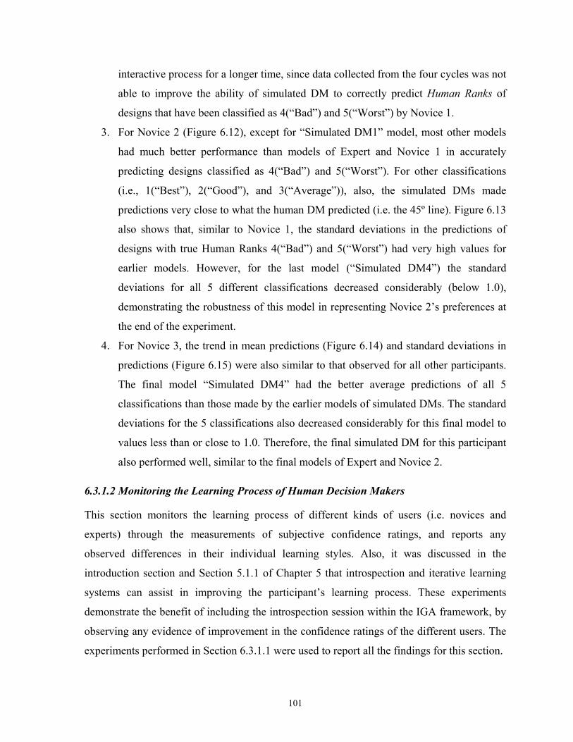
101
interactive process for a longer time, since data collected from the four cycles was not
able to improve the ability of simulated DM to correctly predict Human Ranks of
designs that have been classified as 4(“Bad”) and 5(“Worst”) by Novice 1.
3. For Novice 2 (Figure 6.12), except for “Simulated DM1” model, most other models
had much better performance than models of Expert and Novice 1 in accurately
predicting designs classified as 4(“Bad”) and 5(“Worst”). For other classifications
(i.e., 1(“Best”), 2(“Good”), and 3(“Average”)), also, the simulated DMs made
predictions very close to what the human DM predicted (i.e. the 45º line). Figure 6.13
also shows that, similar to Novice 1, the standard deviations in the predictions of
designs with true Human Ranks 4(“Bad”) and 5(“Worst”) had very high values for
earlier models. However, for the last model (“Simulated DM4”) the standard
deviations for all 5 different classifications decreased considerably (below 1.0),
demonstrating the robustness of this model in representing Novice 2’s preferences at
the end of the experiment.
4. For Novice 3, the trend in mean predictions (Figure 6.14) and standard deviations in
predictions (Figure 6.15) were also similar to that observed for all other participants.
The final model “Simulated DM4” had the better average predictions of all 5
classifications than those made by the earlier models of simulated DMs. The standard
deviations for the 5 classifications also decreased considerably for this final model to
values less than or close to 1.0. Therefore, the final simulated DM for this participant
also performed well, similar to the final models of Expert and Novice 2.
6.3.1.2 Monitoring the Learning Process of Human Decision Makers
This section monitors the learning process of different kinds of users (i.e. novices and
experts) through the measurements of subjective confidence ratings, and reports any
observed differences in their individual learning styles. Also, it was discussed in the
introduction section and Section 5.1.1 of Chapter 5 that introspection and iterative learning
systems can assist in improving the participant’s learning process. These experiments
demonstrate the benefit of including the introspection session within the IGA framework, by
observing any evidence of improvement in the confidence ratings of the different users. The
experiments performed in Section 6.3.1.1 were used to report all the findings for this section.
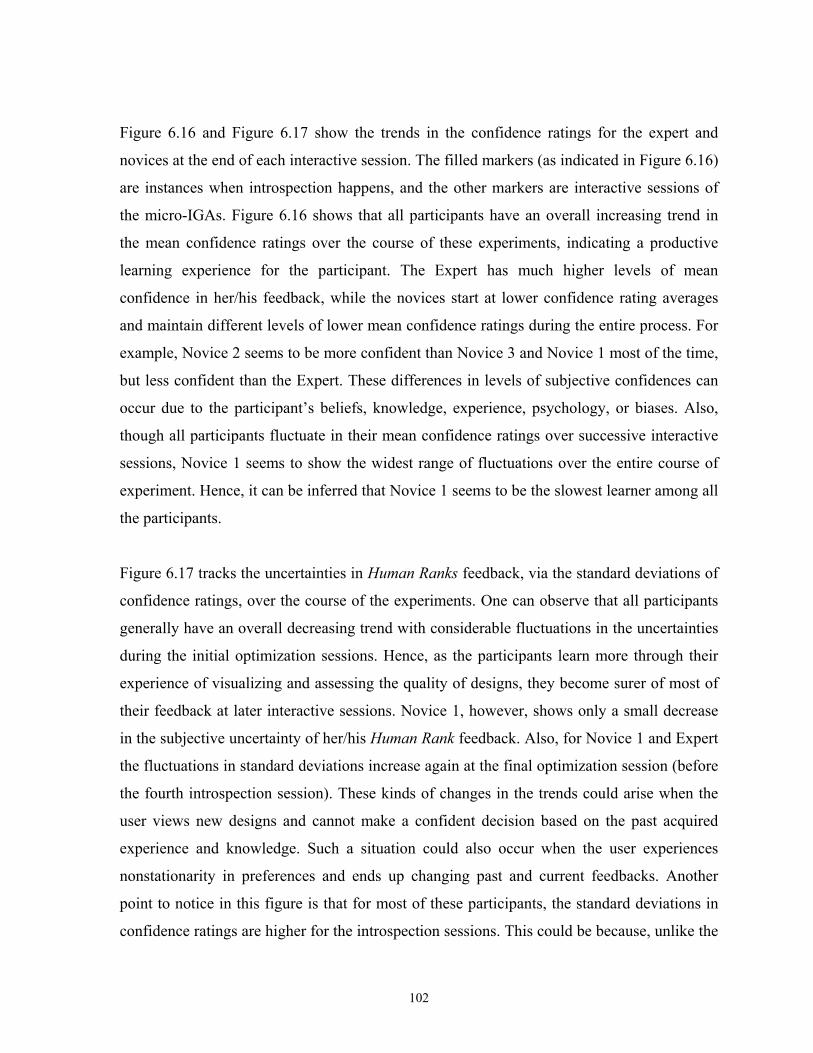
102
Figure 6.16 and Figure 6.17 show the trends in the confidence ratings for the expert and
novices at the end of each interactive session. The filled markers (as indicated in Figure 6.16)
are instances when introspection happens, and the other markers are interactive sessions of
the micro-IGAs. Figure 6.16 shows that all participants have an overall increasing trend in
the mean confidence ratings over the course of these experiments, indicating a productive
learning experience for the participant. The Expert has much higher levels of mean
confidence in her/his feedback, while the novices start at lower confidence rating averages
and maintain different levels of lower mean confidence ratings during the entire process. For
example, Novice 2 seems to be more confident than Novice 3 and Novice 1 most of the time,
but less confident than the Expert. These differences in levels of subjective confidences can
occur due to the participant’s beliefs, knowledge, experience, psychology, or biases. Also,
though all participants fluctuate in their mean confidence ratings over successive interactive
sessions, Novice 1 seems to show the widest range of fluctuations over the entire course of
experiment. Hence, it can be inferred that Novice 1 seems to be the slowest learner among all
the participants.
Figure 6.17 tracks the uncertainties in Human Ranks feedback, via the standard deviations of
confidence ratings, over the course of the experiments. One can observe that all participants
generally have an overall decreasing trend with considerable fluctuations in the uncertainties
during the initial optimization sessions. Hence, as the participants learn more through their
experience of visualizing and assessing the quality of designs, they become surer of most of
their feedback at later interactive sessions. Novice 1, however, shows only a small decrease
in the subjective uncertainty of her/his Human Rank feedback. Also, for Novice 1 and Expert
the fluctuations in standard deviations increase again at the final optimization session (before
the fourth introspection session). These kinds of changes in the trends could arise when the
user views new designs and cannot make a confident decision based on the past acquired
experience and knowledge. Such a situation could also occur when the user experiences
nonstationarity in preferences and ends up changing past and current feedbacks. Another
point to notice in this figure is that for most of these participants, the standard deviations in
confidence ratings are higher for the introspection sessions. This could be because, unlike the

103
interactive sessions of the micro-IGAs that evaluate standard deviations of the current
optimization population, the introspection sessions evaluate standard deviations for all the
previously found solutions. When previous solutions (in the HDMA or the CBM) with low
confidence ratings are not re-evaluated by the participant, the overall uncertainty in the
subjective confidence of the entire population adds to the standard deviation calculated after
the introspection session. However, in spite of these peaks of uncertainty in confidence
ratings, the overall decreasing trend for all standard deviations evaluated for the introspection
sessions demonstrate the improvement in the learning from the participants’ perspective.
For a statistical analysis of the observed standard deviations of confidence ratings, Mann-
Kendall test was performed for all four time periods that start from the first interactive
session and end after every introspection session. Table 6.1 reports the Mann-Kendall
statistics for each of the participants. Also, recall that in the methodology section (Section
6.2.4 and Figure 6.7) the transition of significance levels of the decreasing trends detected in
the standard deviations was used by the proposed adaptive strategy to guide the MIM in
managing the initiative between human and simulated DMs. Column 2 of this table lists the
Kendall’s statistic S (Equation 6.1), in which the negative values indicate a decreasing trend
detected in the dataset. Column 3 lists the bounds (in Section 6.2.2) within which the
statistical significance level (i.e. α) for these trends lie. As observed in column 3 of this table,
all participants generally show improvements in the significance levels of the decreasing
trend as learning progresses. This indicates improvement in learning, which further confirms
the observations of the Figure 6.16 and Figure 6.17 in the previous paragraph. However, for
Expert, Novice 1, Novice 2, and Novice 3 at the end of their fourth, third, third, and third
introspection sessions respectively, the significance level for making a Type 1 error (i.e.
when the null hypothesis that indicates no change in the mean of the data, is incorrectly
rejected) increased in comparison to the significance level of the previous introspection
session. These can be related to the increased fluctuations in the standard deviations of
confidence ratings for the micro-IGAs just before these introspection sessions. In context of
the human’s learning performance and the MIM, this increase in the probability of errors
would necessitate a further investment of the human DM’s involvement. Since the IGAMII is
also used as a learning tool by the human DM, additional experience with the interactive
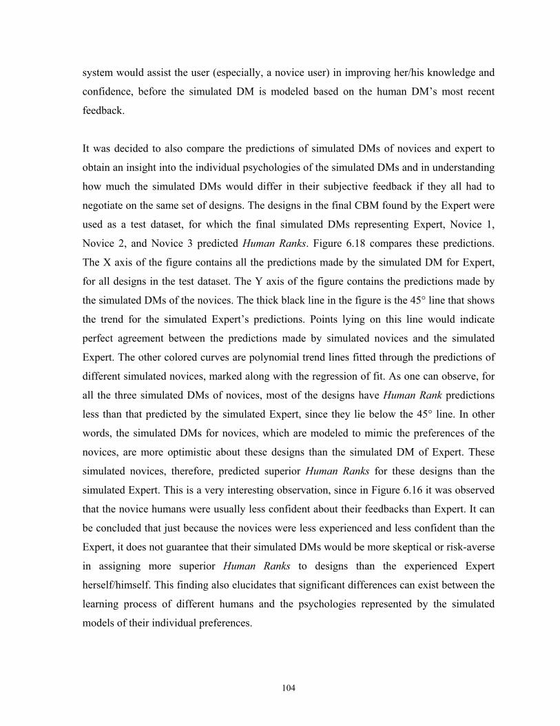
104
system would assist the user (especially, a novice user) in improving her/his knowledge and
confidence, before the simulated DM is modeled based on the human DM’s most recent
feedback.
It was decided to also compare the predictions of simulated DMs of novices and expert to
obtain an insight into the individual psychologies of the simulated DMs and in understanding
how much the simulated DMs would differ in their subjective feedback if they all had to
negotiate on the same set of designs. The designs in the final CBM found by the Expert were
used as a test dataset, for which the final simulated DMs representing Expert, Novice 1,
Novice 2, and Novice 3 predicted Human Ranks. Figure 6.18 compares these predictions.
The X axis of the figure contains all the predictions made by the simulated DM for Expert,
for all designs in the test dataset. The Y axis of the figure contains the predictions made by
the simulated DMs of the novices. The thick black line in the figure is the 45° line that shows
the trend for the simulated Expert’s predictions. Points lying on this line would indicate
perfect agreement between the predictions made by simulated novices and the simulated
Expert. The other colored curves are polynomial trend lines fitted through the predictions of
different simulated novices, marked along with the regression of fit. As one can observe, for
all the three simulated DMs of novices, most of the designs have Human Rank predictions
less than that predicted by the simulated Expert, since they lie below the 45° line. In other
words, the simulated DMs for novices, which are modeled to mimic the preferences of the
novices, are more optimistic about these designs than the simulated DM of Expert. These
simulated novices, therefore, predicted superior Human Ranks for these designs than the
simulated Expert. This is a very interesting observation, since in Figure 6.16 it was observed
that the novice humans were usually less confident about their feedbacks than Expert. It can
be concluded that just because the novices were less experienced and less confident than the
Expert, it does not guarantee that their simulated DMs would be more skeptical or risk-averse
in assigning more superior Human Ranks to designs than the experienced Expert
herself/himself. This finding also elucidates that significant differences can exist between the
learning process of different humans and the psychologies represented by the simulated
models of their individual preferences.

105
The learning process of the four participants was also compared to the trends in the
performance of the simulated DMs (Section 6.3.1.2) to examine any relationship between
them. In Section 6.3.1.2 it was observed that earlier models (e.g. “Simulated DM1” and
“Simulated DM2”) had much higher errors in classifications of designs. In relation to the
learning process of participants, during the early introspection sessions the participants also
had significant fluctuations in the standard deviations of their confidence ratings (Figure
6.17). Therefore, during the early phases of the experiment, both human DM and simulated
DM were still in the premature stage of learning. Also, at the end of the experiment, the final
model of the participants (except for Novice 1) had average Human Rank predictions close to
the predictions made by human DM (i.e. standard deviations less than 1.0), and during this
period improvement in the confidence ratings (Figures 6.16 and 6.17) of the participants was
also observed. One might argue that perhaps the simulated DMs performed better during later
training sessions because of larger collection of training examples, which the earlier models
did not have; however, the learning process of Novice 1 and the prediction performance of
simulated DMs for Novice 1 contradict this argument. As seen by Figure 6.17, Novice 1 had
very little decrease in the uncertainty of her/his confidence ratings. This participant also had
a slow learning process and showed considerable and consistent fluctuations in the reliability
of her/his feedback, during the entire experiment. High fluctuations in confidence rating
exhibit her/his susceptibility to change Human Ranks of these designs at a later instance in
time. For “Simulated DM4” of Novice 1, at the end of the experiment – even though there
was a large collection of training examples (similar to the amount present for other
participants) – the predictions for designs classified as 1(“Best”), 4(“Bad”), and 5(“Worst”)
by the human DM had moderate values of standard deviations (greater than 1.0). In
summary, it can be inferred that extensive disruptions in the Novice 1’s feedback affected the
training of the simulated DM. Hence, it is important for an interactive system to allow the
learning process of human DM to mature through the process of optimization-introspection,
so that only consistent and reliable feedback from the human DM is utilized to create models
of simulated DMs. Further study on learning pattern of decision makers and the
corresponding effect on the training of simulated DMs could assist in the categorization of
the disruptions that originate from the lag in the human DM’s learning process.
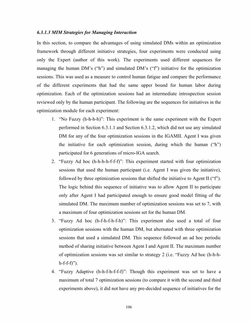
106
6.3.1.3 MIM Strategies for Managing Interaction
In this section, to compare the advantages of using simulated DMs within an optimization
framework through different initiative strategies, four experiments were conducted using
only the Expert (author of this work). The experiments used different sequences for
managing the human DM’s (“h”) and simulated DM’s (“f”) initiative for the optimization
sessions. This was used as a measure to control human fatigue and compare the performance
of the different experiments that had the same upper bound for human labor during
optimization. Each of the optimization sessions had an intermediate introspection session
reviewed only by the human participant. The following are the sequences for initiatives in the
optimization module for each experiment:
1. “No Fuzzy (h-h-h-h)”: This experiment is the same experiment with the Expert
performed in Section 6.3.1.1 and Section 6.3.1.2, which did not use any simulated
DM for any of the four optimization sessions in the IGAMII. Agent I was given
the initiative for each optimization session, during which the human (“h”)
participated for 6 generations of micro-IGA search.
2. “Fuzzy Ad hoc (h-h-h-h-f-f-f)”: This experiment started with four optimization
sessions that used the human participant (i.e. Agent I was given the initiative),
followed by three optimization sessions that shifted the initiative to Agent II (“f”).
The logic behind this sequence of initiative was to allow Agent II to participate
only after Agent I had participated enough to ensure good model fitting of the
simulated DM. The maximum number of optimization sessions was set to 7, with
a maximum of four optimization sessions set for the human DM.
3. “Fuzzy Ad hoc (h-f-h-f-h-f-h)”: This experiment also used a total of four
optimization sessions with the human DM, but alternated with three optimization
sessions that used a simulated DM. This sequence followed an ad hoc periodic
method of sharing initiative between Agent I and Agent II. The maximum number
of optimization sessions was set similar to strategy 2 (i.e. “Fuzzy Ad hoc (h-h-h-
h-f-f-f)”).
4. “Fuzzy Adaptive (h-h-f-h-f-f-f)”: Though this experiment was set to have a
maximum of total 7 optimization sessions (to compare it with the second and third
experiments above), it did not have any pre-decided sequence of initiatives for the

107
human or the simulated expert. The adaptive strategy, proposed earlier in this
chapter, chose the real-time sequence h-h-f-h-f-f-f for the Expert’s (“h”) and the
simulated DM’s (“f”) initiatives based on the Expert’s temporal feedback. Note
that, based on the improvement in confidence ratings trends for this participant,
the MIM decided to shift the initiative to the simulated DM for the optimization
session of third cycle. However, during the introspection session of the third cycle
the human DM expressed an increased uncertainty in her/his confidence in the
Human Ranks of the new solutions found with the assistance of simulated DM.
The MIM, therefore, recommended the shift in initiative back to the human DM
to allow her/him to gain additional learning experience with the problem and the
new emerging solutions.
Other parameter settings for the micro-IGA used by Agent I were fixed to a population size
of 30, maximum number of generations of 6, uniform crossover rate of 0.75, and mutation
rate of 0.03. GA parameter settings for the IGA used by Agent II had a population size of
100, maximum number of generations of 24, uniform crossover rate of 0.75, and mutation
rate of 0.01. Both Agent I and Agent II had their starting populations injected with solutions
from the CBM by using the tournament selection scheme based on Pareto ranks and
crowding distance (refer to Step 3 of Section 5.2.1 for details). The number of CBM
solutions selected for Agent I and Agent II was 20% of the population size used by Agent I.
Figure 6.19 reports the number of above-average solutions (Human Rank < 3) found by the
different experiments. When no simulated DM is involved during optimization (i.e. “No
Fuzzy (h-h-h-h)” experiment), the number of above-average solutions found was 12, which is
86%, 78%, and 90% less than the number found by “Fuzzy Ad hoc (h-h-h-h-f-f-f)”, “Fuzzy
Ad hoc (h-f-h-f-h-f-h)”, and “Fuzzy Adaptive (h-h-f-h-f-f-f)”, respectively. This
demonstrates the advantages of using a simulated DM along with the human DM within the
optimization process. The adaptive strategy “Fuzzy Adaptive (h-h-f-h-f-f-f)” monitored the
confidence ratings of Expert and used the simulated DM’s initiative during the appropriate
time to produce the largest number of above-average designs (i.e. 120 designs). Ad hoc
strategies, i.e. experiment 2 and 3, found only 84 and 53 above-average designs. Also, for ad
108
hoc strategies, since it was unknown when the right time to include the simulated DM’s
initiative would arise, the human participated in four optimization sessions. The adaptive
strategy, on the other hand, used the human DM for only three optimization sessions
(equivalent to a decrease in human effort involved during evaluation of 180 designs). The
adaptive strategy was able to monitor the rapid improvement in the human’s learning process
via the confidence ratings and use the human’s initiative only when the strategy observed
instances of low average confidence ratings or increase in uncertainty of user’s subjective
confidence.
Figures 6.20, 6.21, and 6.22 compare the objective space for above-average designs found in
the three experiments involving simulated DMs relative to the first experiment with no
simulated DM. It is clearly evident that all strategies that utilize the simulated DM (i.e.
experiments 2, 3, and 4) found a more diverse distribution of above-average designs than the
strategy that used no simulated DM (i.e. experiment 1: “No Fuzzy (h-h-h-h)”). Along the X
axis (i.e. “Number of Wells”) the distribution of diverse above-average solutions is
comparable for ad hoc and adaptive strategies using simulated DMs. However, along the Y
axis (i.e. Benzene Error), “Fuzzy Ad hoc (h-h-h-h-f-f-f)” and “Fuzzy Adaptive (h-h-f-h-f-f-
f)” fare much better in finding a diverse set of above-average solutions, than “Fuzzy Ad hoc
(h-f-h-f-h-f-h)”. Multiple experiments with different users would be needed to determine why
“Fuzzy Ad hoc (h-f-h-f-h-f-h)” did not perform as well as the other techniques that used
simulated DMs. It can, however, be inferred that since “Fuzzy Ad hoc (h-f-h-f-h-f-h)”
alternated initiatives of human DM and simulated DM irrespective of the learning process,
untimely use of simulated DM when the learning process of human DM was rudimentary
could have led the optimization method to search for solutions that were mistakenly
identified as above-average initially and were corrected to be average or below-average near
or at the end of the experiment. On the other hand, though “Fuzzy Ad hoc (h-h-h-h-f-f-f)” did
not monitor the learning process of the human DM, it did however provide the human DM
ample time to learn about her/his subjective feedback before the modeled simulated DM was
utilized for optimization. “Fuzzy Adaptive (h-h-f-h-f-f-f)” also used the modeled simulated
DM for optimization when the learning process of the human DM was consistent and
matured. Therefore, both “Fuzzy Ad hoc (h-h-h-h-f-f-f)” and “Fuzzy Adaptive (h-h-f-h-f-f-

109
f)” used simulated DMs that were more accurate representations of the human DM’s
preferences and were able to identify diverse above-average designs effectively.
6.3.2 Application of IGAMII to Groundwater Long-term Monitoring Problem
In the experiments examined for the previous section (i.e. Section 6.3.1), it was deduced that
the proposed adaptive strategy for managing initiative is most suited for real-time
optimization when humans have lags and uncertainties in their learning process. The adaptive
strategy allows the human DM to interact with the system, until the learning process has
matured and the user is confident about the reliability in her/his feedback. Only then does the
strategy allow the modeled simulated DM to represent the human DM’s preferences within
the optimization process. As a final step, the proposed IGAMII strategy was implemented
with one expert and two novices. The author was, once again, the Expert for these
experiments, while two new novices were selected from volunteering graduate students of
the Department of Civil and Environmental Engineering at the University of Illinois at
Urbana-Champaign. In these experiments the maximum number of optimization sessions was
again limited to four and the MIM adaptively decided which agent got the initiative for
interaction. Other IGAMII parameters were similar to the ones used in previous experiments
(i.e. Agent I micro-IGA used 6 generations with population size of 30, uniform crossover rate
of 0.75, and mutation rate of 0.03; Agent II IGA used 24 generations with population size of
100, uniform crossover rate of 0.75, and mutation rate of 0.01). The starting populations of
the IGAs during optimization were created in a same manner as that for the previous
experiments in Section 6.3.1.1.
Figure 6.23 reports the trends in standard deviations of confidence ratings for the three
participants “Expert”, “Novice 4”, and “Novice 5”. The IGAMII identified the following
initiative sequences for the three participants based on their confidence ratings: h-h-f-h for
the Expert, h-h-f-h for Novice 4, and h-h-h-f for Novice 5, where “h” refers to optimization
sessions involving the human DM and “f” refers to optimization sessions involving the
simulated DM. The filled markers in this graph refer to the introspection sessions. It is clear
from the trend in uncertainty of confidence ratings that all participants had fluctuations in
confidence ratings during the first two optimization sessions and, thus, were given the
110
initiative to participate and learn through the process of comparing and ranking solutions.
The IGAMII shifted the initiative to Agent II (which uses the simulated DM) during the third
optimization session for both Expert and Novice 4, but did not trigger a similar shift of
initiative for Novice 5 until the fourth optimization session. This sensitivity of IGAMII to the
changes in trends of confidence ratings of participants allowed the framework to assist the
participant to reach a certain level of confidence in their feedback before the simulated DM
was utilized. Also, for Expert and Novice 4, the IGAMII found a statistical increase in the
variation of their confidence ratings after their third optimization session ended, and thus,
switched the initiative back to human DM for the fourth optimization session. During the
fourth optimization session, the Expert was able to perform much better with respect to
variations in confidence ratings and indicated a fast learning process. However, Novice 4 still
faced considerable fluctuations of the standard deviations, indicating a slower learning
process.
At the end of the experiments, the final solution sets in the CBMs were then compared for the
three participants. The Expert, Novice 4, and Novice 5 found 39, 48, and 27 above-average
designs out of a total of 78, 68, 61 designs, respectively. Qualitative analysis of the designs
was based on the same criteria as explained in Section 6.3.1.1.Figure 6.24 shows the
objective space for all the above-average designs found by the participants. Solutions found
by the participants are also compared with the solutions found by the Non-interactive Genetic
Algorithm (NGA) in Section 5.3.3 of Chapter 5. All participants found a good spread of
diverse solutions that had above-average quality, even though many of their solutions had
worse numerical values for benzene error than NGA solutions. Also, for a particular number
of wells, all participants with the help of their simulated DMs found multiple designs that
met their subjective criteria. Figures 6.25 and Figure 6.26 show the design with all 36 wells
monitored and the NGA solution for 28 monitoring wells, respectively. Figures 6.27, 6.28,
and 6.29 show all above-average designs that these participants found for solutions that use
28 monitoring wells, as an example of the effects of interaction. It is visually evident that the
designs found by all participants preserve the delineation of the BTEX and benzene plumes
better and have fewer abnormal high concentration local zones (also called “hotspots”) than
the designs proposed by NGA, when compared to each other and to the “All Wells” design in
111
Figure 6.25. From these figures it is also apparent that each of these participants had their
individual biases and subjective interpretation of solution quality, and had differences in
opinions in deciding which designs ranked “Best” (Human Rank 1) or “Good” (Human Rank
2). For example, for the 28-wells designs even though all three participants came up with
multiple above-average designs, their actual designs were different from those found by the
other participants. This indicates that negotiation between the participants would be needed if
a particular monitoring plan was chosen for final implementation. This would then require
some systematic conflict resolution procedure for reaching a consensus between the three
participants. Another example of differences in preferences between participants can be
detected in Figure 6.24. In this figure, Novice 4 ranked solutions with number of wells less
than 28 as above-average, even though these solutions had high benzene errors. Expert
ranked solutions with high benzene error as above-average when the number of wells was
more than 28. And Novice 5 seemed to be most risk averse among the three participants,
since the solutions found by this participant did not violate benzene error as high as that of
other participants. Also with respect to human labor, appropriate utilization of the simulated
DM helped the participants to constrain their human labor to only three optimization sessions
for an experiment that would have otherwise utilized human labor for four optimization
sessions.
Since the human participant is an integral part of this interactive search methodology, it was
also decided to collect evaluation information from the novice participants. Below are their
comments that illuminate their personal learning styles and experiences with the IGAMII
system:
Novice 4: “… When I first started the optimization I was very unsure about how I classified
each example. I liked the ability to use the slider bar to indicate my lack of certainty. As I
got further into the optimization, I became more familiar with the range of solutions that I
would see. Because of this, it was nice that I could reevaluate some of the first solutions that
I may have ranked incorrectly during the introspection. Also, as I became more familiar
with the range of solutions that I would see the ranking procedure took less and less time and
I had higher confidence in my rankings.”

112
Novice 5: “… I was fairly confident of my results for the first cycle – the second cycle
showed some additional pictures (the 29 well and 27 well solutions I think) that made me
rethink my 2/3 ranks and 3/4 ranks. By the end of the 3rd cycle, I was quite confident of my
ranking. The fuzzy model showed some additional solutions (30 well and 32 well solutions)
that I felt were as good as the all well solution. These didn’t come up in the earlier
generations – but I hadn’t ranked any other solutions with rank 1, so it didn’t change my
ranking scheme.”
6.4 Conclusions
This chapter initially focused on assessing the learning process of human DMs, i.e. expert
and novices, by using their confidence ratings as a method to monitor their acquisition of
knowledge. It was observed that all human participants, when instructed to perform the same
task, can influence any interactive search process with their own biases, beliefs, and
experience. The novices tend to be more critical of their feedback and thus have lower
confidence ratings than the expert. However, all participants show improvements in their
confidence as their learning improves. The IGAMII was better than the CBMIGA (Chapter
5) and the SIGA (Chapter 4) in its ability to identify multiple diverse above-average designs.
For example, it was observed in Section 6.3.2 that the different participants Expert, Novice 4,
and Novice 5, irrespective of their experience with the LTM problem, were able to use the
IGAMII in finding 39, 48, and 27 above-average designs respectively. Whereas, CBMIGA
(Chapter 5) and SIGA (Chapter 4) assisted the Expert in finding only 18 and 6 diverse above-
average designs, respectively. Figures 6.27, 6.28, and 6.29 show the above-average designs
for monitoring plans with 28 wells that meet the qualitative criteria for plume delineations of
Benzene and BTEX. With IGAMII, Expert found four above-average designs, Novice 4
found nine above-average designs and Novice 5 found five above-average designs which use
28 monitoring wells and do not have spurious high concentrations near the boundaries of the
site. In comparison, the CBMIGA (Chapter 5) was able to assist the Expert in finding three
above-average designs with 28 monitoring wells, while SIGA (Chapter 4) could only find
one above-average design with the same number of wells. Also, many of these sets of diverse
above-average designs were different from those found by the other participants. Therefore,

113
if the site owners had a budget for monitoring 28 wells, then in order to reach a consensus on
the final LTM plan some method for conflict resolution may be needed. This stage of
negotiation between multiple participants who can find robust designs through interactive
optimization will be, however, left as a topic for future research.
The advantages of using ANFIS to create models of nonstationary preferences, as expressed
by the human DMs, were also studied as a next step. However, it was inferred through this
study that, even though ANFIS is a robust algorithm in training the simulated DMs, naïve
application of the simulated DM for optimization would be faulty if the data used for training
did not represent the feedback of a confident human who had reached her/his optimal
learning level.
The next section of the chapter examined various strategies for managing the initiatives for
interaction between the simulated and human DMs. It was determined that the adaptive
mixed-initiative interaction strategy proposed in this work outperformed ad hoc collaboration
strategies in not only judiciously utilizing the feedback from the simulated and human DMs,
but also in decreasing human fatigue by not requiring the human DM to participate when it
was deemed not necessary. For example, in Section 6.3.1.3 the adaptive strategy was able to
save human effort involved in evaluating 180 designs, while the other strategies did not make
any such savings in human effort. Also, “Fuzzy Adaptive (h-h-f-h-f-f-f)” found 90%, 30%,
and 56% more above-average solutions than “No Fuzzy (h-h-h-h)”, “Fuzzy Ad hoc (h-h-h-h-
f-f-f)”, and “Fuzzy Ad hoc (h-f-h-f-h-f-h)” respectively. It was observed that for most
participants the role of the humans changed from being actively involved in optimization to
the role of introspection and review. However, when humans showed a significant change in
their learning pattern, the initiative was shifted back towards the human DMs to allow them
the opportunity to gain vital knowledge.
Overall, this chapter has made an important contribution in not only understanding how real
DMs learn via interactive systems and the advantages of using ANFIS for creating simulated
DMs to control human fatigue, it also has proposed a useful adaptive strategy for managing

114
initiatives for interaction when different multiple agents with their own learning curves are
involved in the interactive search process.
Table 6.1 Mann Kendall statistics for trends in standard deviations of confidence ratings
Expert Introspection Session Mann Kendall, Stest Significance Level End of Session 1 -1 α > 0.1 End of Session 2 -39 0.01< α < 0.025 End of Session 3 -95 α < 0.005 End of Session 4 -129 0.005 < α < 0.01 Novice 1 Introspection Session Mann Kendall, Stest Significance Level End of Session 1 -7 α > 0.1 End of Session 2 -29 0.05 < α < 0.1 End of Session 3 -34 α > 0.1 End of Session 4 -74 0.05 < α < 0.1 Novice 2 Introspection Session Mann Kendall, Stest Significance Level End of Session 1 -18 0.025 < α < 0.05 End of Session 2 -68 α < 0.005 End of Session 3 -100 0.005 < α < 0.01 End of Session 4 -214 α < 0.005 Novice 3 Introspection Session Mann Kendall, Stest Significance Level End of Session 1 -7 α > 0.1 End of Session 2 -38 0.01 < α < 0.025 End of Session 3 -60 0.025 < α <0.05 End of Session 4 -132 α < 0.005

115
400
500
600
700
800
900
1000
1100
1200
1300
1400
1300 1500 1700 1900 2100 2300 2500 2700 2900X, ft
Y, ft
Monitoring Well LocationsCentral Region Boundary
Figure 6.1 Central region used for creating the Simulated DM
Figure 6.2 Simulated DM: Membership functions for Benzene Error objective
Figure 6.3 Simulated DM: Membership functions for Number of Wells

116
Figure 6.4 Simulated DM: Membership functions for Benzene Error in Central Region
Figure 6.5 Simulated DM: Membership functions for BTEX Error in Central Region

117
MIXED-INITIATIVE MANAGER
( Selects either method I or II for optimization)
Simulated DM Models
Human DM Archive
Case Based Memory
Small population MicroIGA with Human DM
Case Based Memory Interface
Human DM Initiative
Simulated DM Initiative
Human DM Interacti on
Human DM Archived Solutions
Interface
Human DM Interaction
Agent I Agent II
OPTIMIZATION
INTROSPECTION
Medium/Large population IGA with Simulated DM
Figure 6.6 Interactive Genetic Algorithm with Mixed Initiative Interaction

118
Are there enough training examples in HDMA?
Update Simulated DM model
Is testing error of new model ≤ old model?
Use New Model for simulated DM
Use Old Model for simulated DM
Is average confidence rating of latest introspection session ≥ Threshold value?
Use Human DM initiative
Use Simulated DM initiative
Is trend in standard deviation of confidence rating decreasing?
Has significance level of standard deviation trend improved since the last introspection
Start
Obtain initiative
Obtain next model for simulated DM
No
Yes
Yes
Yes
No
Yes
No
No
No
No
Yes
Figure 6.7 Flowchart for controlling initiatives using the proposed adaptive Mixed Initiative Interaction strategy
Yes

119
0
1
2
3
4
5
6
0 1 2 3 4 5 6
Mean of Actual Human Ranks assigned by Expert Human DM
Mea
n H
uman
Ran
ks p
redi
cted
by
Sim
ulat
ed D
Ms
Simulated DM1 Simulated DM2 Simulated DM3 Simulated DM4 45-degree line
Figure 6.8 Average of Human Ranks predictions made by simulated DMs of Expert, at consecutive training sessions
0
2
4
6
8
10
12
14
16
18
20
Simulated DM 1 Simulated DM 2 Simulated DM 3 Simulated DM 4
Simulated DMs for Expert
Stan
dard
Dev
iatio
ns in
Hum
an R
anks
pre
dict
ions
Human Rank 1Human Rank 2Human Rank 3Human Rank 4Human Rank 5
Figure 6.9 Standard deviation of Human Ranks predictions made by simulated DMs of Expert, at consecutive training sessions

120
0
1
2
3
4
5
6
7
8
9
10
0 1 2 3 4 5 6
Mean of Actual Human Ranks assigned by Novice 1 Human DM
Mea
n H
uman
Ran
ks p
redi
cted
by
Sim
ulat
ed D
Ms
Simulated DM1 Simulated DM2 Simulated DM3 Simulated DM4 45-degree line
Figure 6.10 Average of Human Ranks predictions made by simulated DMs of Novice 1, at consecutive training sessions
0
2
4
6
8
10
12
14
16
18
20
Simulated DM 1 Simulated DM 2 Simulated DM 3 Simulated DM 4
Simulated DMs for Novice 1
Stan
dard
Dev
iatio
ns in
Hum
an R
anks
pre
dict
ions
Human Rank 1Human Rank 2Human Rank 3Human Rank 4Human Rank 5
Figure 6.11 Standard deviation of Human Ranks predictions made by simulated DMs of Novice 1, at consecutive training sessions

121
-1
0
1
2
3
4
5
6
0 1 2 3 4 5 6
Mean of Actual Human Ranks assigned by Novice 2 Human DM
Mea
n H
uman
Ran
ks p
redi
cted
by
Sim
ulat
ed D
Ms
Simulated DM1 Simulated DM2 Simulated DM3 Simulated DM4 45-degree line
Figure 6.12 Average of Human Ranks predictions made by simulated DMs of Novice 2, at consecutive training sessions
0
2
4
6
8
10
12
14
16
18
20
Simulated DM 1 Simulated DM 2 Simulated DM 3 Simulated DM 4
Simulated DMs for Novice 2
Sta
ndar
d D
evia
tions
in H
uman
Ran
ks p
redi
ctio
ns
Human Rank 1Human Rank 2Human Rank 3Human Rank 4Human Rank 5
Figure 6.13 Standard deviation of Human Ranks predictions made by simulated DMs of Novice 2, at consecutive training sessions

122
0
1
2
3
4
5
6
7
8
0 1 2 3 4 5 6
Mean of Actual Human Ranks assigned by Novice 3 Human DM
Mea
n H
uman
Ran
ks p
redi
cted
by
Sim
ulat
ed D
Ms
Simulated DM1 Simulated DM2 Simulated DM3 Simulated DM4 45-degree line
Figure 6.14 Average of Human Ranks predictions made by simulated DMs of Novice 3, at consecutive training sessions
0
2
4
6
8
10
12
14
16
18
20
Simulated DM 1 Simulated DM 2 Simulated DM 3 Simulated DM 4
Simulated DMs for Novice 3
Sta
ndar
d D
evia
tions
in H
uman
Ran
ks p
redi
ctio
ns
Human Rank 1Human Rank 2Human Rank 3Human Rank 4Human Rank 5
Figure 6.15 Standard deviation of Human Ranks predictions made by simulated DMs of Novice 3, at consecutive training sessions

123
0.6
0.65
0.7
0.75
0.8
0.85
0.9
0.95
1
0 5 10 15 20 25 30 35
Interactive Session
Mea
n
Expert
Novice 1
Novice 2
Novice 3
Figure 6.16 Mean confidence ratings at end of every interactive session, for expert and novices
0
0.05
0.1
0.15
0.2
0.25
0.3
0 5 10 15 20 25 30 35
Interactive Session
Stan
dard
Dev
iatio
n ExpertNovice 1
Novice 2Novice 3
Figure 6.17 Standard deviations of confidence ratings at end of every interactive session, for expert and novices
Introspection Sessions

124
Simulated Novice 1: R2 = 0.4927
Simulated Novice 2: R2 = 0.8479
Simulated Novice 3: R2 = 0.7899
1
2
3
4
5
1 2 3 4 5
Human Rank predictions of the Simulated Expert
Hum
an R
ank
pred
ictio
ns o
f Sim
ulat
ed N
ovic
es
Simulated Novice 1 Simulated Novice 2 Simulated Novice 3 45-degree line
Figure 6.18 Comparison of simulated expert and simulated novices
0
20
40
60
80
100
120
140
No Fuzzy (h-h-h-h)
Fuzzy Ad hoc(h-h-h-h-f-f-f)
Fuzzy Ad hoc(h-f-h-f-h-f-h)
Fuzzy Adaptive(h-h-f-h-f-f-f)
Num
ber o
f abo
ve-a
vera
ge d
esig
ns
Figure 6.19 Performance of initiative strategies for Expert

125
0
20
40
60
80
100
120
140
160
180
24 26 28 30 32 34 36
Number of Wells
Ben
zene
Err
or -
ppb
No Fuzzy (h-h-h-h)
Fuzzy Ad hoc (h-h-h-h-f-f-f)
Figure 6.20 Comparison of above-average solutions found with no participation of simulated Expert and with ad hoc participation strategy “Fuzzy Ad hoc (h-h-h-h-f-f-f)”
0
20
40
60
80
100
120
140
24 26 28 30 32 34 36
Number of Wells
Ben
zene
Err
or -
ppb
No Fuzzy (h-h-h-h)
Fuzzy Ad hoc (h-f-h-f-h-f-h)
Figure 6.21 Comparison of above-average solutions found with no participation of simulated Expert and with ad hoc participation strategy “Fuzzy Ad hoc (h-f-h-f-h-f-h)”
0
20
40
60
80
100
120
140
24 26 28 30 32 34 36
Number of Wells
Ben
zene
Err
or -
ppb
No Fuzzy (h-h-h-h)
Fuzzy Adaptive (h-h-f-h-f-f-f)
Figure 6.22 Comparison of above-average solutions found with no participation of simulated Expert and with ad hoc participation strategy “Fuzzy Adaptive (h-h-f-h-f-f-f)”
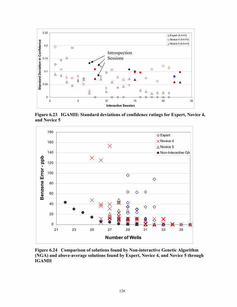
126
0
0.05
0.1
0.15
0.2
0.25
0 5 10 15 20 25
Interactive Session
Stan
dard
Dev
iatio
n in
Con
fiden
ceExpert (h-h-f-h)Novice 4 (h-h-f-h)Novice 5 (h-h-h-f)
Figure 6.23 IGAMII: Standard deviations of confidence ratings for Expert, Novice 4, and Novice 5
0
20
40
60
80
100
120
140
160
180
21 23 25 27 29 31 33 35
Number of Wells
Ben
zene
Err
or -
ppb
Expert
Novice 4
Novice 5
Non-Interactive GA
Figure 6.24 Comparison of solutions found by Non-interactive Genetic Algorithm (NGA) and above-average solutions found by Expert, Novice 4, and Novice 5 through IGAMII
Introspection Sessions

127
Figure 6.25 “All Wells” Solutions: Kriged maps for Benzene and BTEX plumes when all 36 wells are installed, concentration units in ppb. Region enclosed by rectangular box is used for model input of Simulated DM 28 Wells Benzene (ppb) BTEX (ppb) NGA
Figure 6.26 28-wells design found by Non-interactive Genetic Algorithm (NGA) . “o” are locations with active monitoring wells, “+” are locations with monitoring wells shut off.

128
28 Wells Expert
Benzene (ppb) BTEX (ppb)
IGAMII Human Rank 1
IGAMII Human Rank 2
IGAMII Human Rank 2
IGAMII Human Rank 2
Figure 6.27 IGAMII: 28-wells designs found by Expert. “o” are locations with active monitoring wells, “+” are locations with monitoring wells shut off.

129
28 Wells Novice 4
Benzene (ppb) BTEX (ppb)
IGAMII Human Rank 1
IGAMII Human Rank 1
IGAMII Human Rank 1
IGAMII Human Rank 1
IGAMII Human Rank 2
IGAMII Human Rank 2
(Continued on next page)

130
IGAMII Human Rank 2
IGAMII Human Rank 2
IGAMII Human Rank 2
Figure 6.28, cont. IGAMII: 28-wells designs found by Novice 4. “o” are locations with active monitoring wells, “+” are locations with monitoring wells shut off.

131
28 Wells Novice 5
Benzene (ppb) BTEX (ppb)
IGAMII Human Rank 2
IGAMII Human Rank 2
IGAMII Human Rank 2
IGAMII Human Rank 2
IGAMII Human Rank 2
Figure 6.29 IGAMII: 28-wells designs found by Novice 5. “o” are locations with active monitoring wells, “+” are locations with monitoring wells shut off.

132
Chapter 7
7 CONCLUDING REMARKS
This chapter summarizes important conclusions of this research in the first section, followed
by a section that proposes future extensions of this work.
7.1 Summary of Research Findings
The main focus of this research has been in exploring optimization methodologies, which
include subjective criteria of a decision maker (DM) within the search process through
continual online interaction with the DM. The design of the interactive systems was based on
the Genetic Algorithm optimization technique. Effects of various human factors, such as
human fatigue, nonstationarity in preferences, and the cognitive learning process of the
human, were also addressed while constructing such systems.
The advantage of the interactive optimization method in including subjective criteria, which
are not easily expressed using mathematical formal models, was first demonstrated in
Chapter 4. For the groundwater long-term monitoring (LTM) case study, the designs found
by the Standard Interactive Genetic Algorithm (SIGA) satisfied the subjective criteria of the
decision maker better than the Non-interactive Genetic Algorithm (NGA). Though the
designs proposed by SIGA had slightly worse numerical values for one of the formal
objectives (i.e. benzene error) than the designs proposed by NGA, the plume interpolation
maps of SIGA designs respected the spatial attributes along the boundary of the site and in
the high concentration zones (“hotspots”). Therefore, the DM preferred the designs proposed
by SIGA to designs proposed by NGA.
Further in Chapter 5, the proposed Case-Based Micro Interactive Genetic Algorithm
(CBMIGA) outperformed SIGA by proposing multiple solutions, which respected the DM’s
subjective criteria and were above-average designs from the DM’s perspective. For example
for the LTM problem, NGA found one 27-well solution, one 28-well solution, and one 29-
well solution, none of which were above-average. SIGA found more solutions than NGA, but

133
only one 27-well design was above-average, one 28-well design was above-average, and one
29-well design was above-average. However, CBMIGA found multiple solutions that had
three above-average designs with 28 wells, three above-average designs with 27 wells, and
five above-average designs with 29 wells. IGAMII also found multiple above-average
designs for different kinds of users. From the LTM design perspective this is a very useful
result of the CBMIGA and IGAMII frameworks because it allows the expert to select among
several strong candidate designs, depending on her/his LTM budget. For example, if the DM
has a budget with an upper limit of monitoring costs equivalent to monitoring 29 wells, then
she/he can choose from a set of multiple high performance designs with 29 or fewer wells
that have good plume delineation quality and better well support in the north-northeast region
of the site. The non-interactive GA, however, would not be able to propose any robust
solutions within that budget, since none of the proposed designs (with number of wells equal
to or less than 29) satisfied the DM’s preference criteria. For the next stage of decision
making, the DM would present the results of this research to the team of stakeholders and
regulators, who would select one of the candidate monitoring plans through negotiation and
discussion. Various group decision support systems (Desanctis and Gallpe, 1987) are
recommended to assist in the negotiation process through conflict resolution.
The second important finding of this work is that although human fatigue during interaction
can limit the size of populations used by IGA frameworks, introducing pre-optimized
solutions in the starting population of IGAs can assist in providing good starting points to the
search process. Chapter 4 proposed and compared various starting strategies based on their
computational effort and ability to assist small population IGAs in finding more above-
average designs. Systematic sizing of small populations for IGAs was also explored, based
on existing empirical work in the field of Genetic Algorithms. These sizing strategies provide
useful guidelines for practitioners to effectively design their IGA frameworks. Chapter 5
extended the applicability of these starting strategies by creating a case-based memory
(CBM) from evolving robust solutions during the IGA process. Solutions added to the CBM
were reused periodically by introducing them into the starting population of micro-IGAs.
This modification considerably improved the performance of the interactive search process in
finding above-average solutions. For the same level of human DM labor, CBMIGA found 18

134
above-average diverse solutions, while SIGA proposed only 6 above-average solutions. In
Chapter 6, the advanced Interactive Genetic Algorithm with Mixed Initiative Interaction
(IGAMII) framework demonstrated the advantages of using a simulated DM along with a
human DM to control human labor, by opportunistically replacing the human DM with a
simulated DM during the optimization. Also, the use of a simulated DM within the IGA
search process removes the need to limit population size to small values. For example, a
population size of 30 was implemented for the LTM problem when the human DM was
involved. However, with the simulated DM the population size was increased to 100. By
using a much larger population, the simulated DM was able to search the decision space
more rigorously for multiple solutions that met the human DM’s modeled subjective criteria.
For example, in one of the experiments IGAMII used only 75% of the human effort required
for CBMIGA and SIGA and found 120 above-average solutions, for the same user who
participated in the CBMIGA and SIGA experiments.
The effect of the human’s learning process on the functioning of the IGA frameworks was
also studied. It was realized that the human makers construct their own knowledge of a
system based on their experiences and mistakes, whether from prior knowledge or
knowledge gained during the interactive process. During this process decision makers can
alter their reasoning strategies as they spend more time analyzing the problem, and re-
evaluating their feedback and its consequences. Such manner of adaptive decision making
can lead to nonstationarity in preferences, and thus nonstationarity in the human feedback.
Though the SIGA is not designed to handle such nonstationarity in human feedback, the
CBMIGA and IGAMII were designed to handle various disruptions in the search process due
to the time dependant feedback. Both these frameworks used a case-based memory for
introspection and to externally store previously found good solutions whose building block
information was used to search for new robust solutions when the preferences changed.
Moreover, IGAMII was also able to automatically detect and respond to such temporal
changes in the human’s learning process by monitoring the trends in the human’s subjective
confidences. It was observed that as the human participants learn more through their
experience of visualizing and assessing the quality of designs, they became more confident of
their feedbacks at later interactive sessions and as a result their mean confidence ratings rose.

135
The IGAMII also monitored the standard deviations in confidence ratings to assess the
temporal uncertainty in the confidence ratings. It was observed that during initial
optimization sessions all participants have considerable fluctuations in the decreasing trends
of their uncertainties in the evaluation of Human Ranks, which smoothen during later
optimization sessions. This observation not only indicated the benefits of the introspection-
based learning process, but also demonstrated a possible correlation between the confidence
of the human DM and the performance of the simulated DM models. In Chapter 6 it was
observed that as the confidence ratings (both mean and standard deviation) of the participants
improved with time, the performance of their simulated DM in accurately classifying designs
into appropriate Human Ranks also showed a corresponding improvement. For some
participants the fluctuations in standard deviations increased again in later optimization
sessions, which imply that when the user viewed new designs he/she could not make a
confident decision based on the experience and knowledge acquired through the previous
learning process. Such a situation could have also occurred when the user experienced
nonstationarity in preferences and changed past and current feedbacks.
Another important finding is related to the benefit of using an Adaptive-Network-based
Fuzzy Inference System (ANFIS) to create and update a Takagi-Sugeno Fuzzy Inference
(TSFI) based model of the human decision maker’s feedback (Chapter 6). For the LTM
problem, the ANFIS was able to correlate the important fuzzy inputs (i.e. interpolation errors
in global and local regions, and monitoring cost) related to the DM’s criteria for decision
making with the feedback (i.e. Human Ranks) collected during the interactive sessions. For
most participants (both expert and novice type), the final models at the end of the
experiments had average predictions of all 5 Human Ranks classifications (i.e., 1(“Best”),
2(“Good”), and 3(“Average”), 4(“Bad”) and 5(“Worst”)) considerably more accurate than
the earlier models of simulated DMs. The standard deviations for the 5 classifications also
decreased considerably for this final model to values less than or close to 1.0. Differences in
the nature of predictions of simulated DMs for novices and an expert were also observed. For
example, in Chapter 6 it was found that even though the human novices were less confident
than the Expert about their own feedback, the simulated DMs for the novices were more
optimistic than the simulated Expert about the quality of the solutions found by the Expert.

136
This finding also illuminates the characteristics of learning processes of different humans
(e.g., novices and experts) and the psychologies represented by the simulated DMs.
Finally, based on the results of research, the following recommendations are made regarding
the implementation of the three frameworks for solving future problems. Not all problems
need to be solved via interactive optimization techniques. Any practitioner should first
analyze all of the important criteria related to her/his application, and then formulate relevant
objectives and constraints to represent the domain knowledge of the problem within a non-
interactive optimization approach. Since computational evaluations are much cheaper and
faster than human evaluation, human labor should only be utilized when such non-interactive
procedures (such as a non-interactive GA) are unsuccessful in proposing satisfactory designs.
If the DM does identify a need for interactive optimization, due to limitations in accurate
representation of the domain knowledge through quantitative objectives and constraints, then
the choice of CBMIGA or IGAMII would be better than SIGA because both CBMIGA and
IGAMII outperformed SIGA. However, since CBMIGA does not require the design and
creation of a simulated DM, the DM might find it more convenient to first utilize CBMIGA.
However, IGAMII is much more effective in reducing human fatigue than CBMIGA.
Therefore, if the DM discovers that she/he is still not satisfied with the quality of the
solutions proposed by CBMIGA, then she/he might want to consider spending some human
effort in creating a suitable simulated DM model and then inserting it into an IGAMII
framework that can automatically update the model parameters of the simulated DM and
perform a much more exhaustive search using larger populations and decreased human labor.
7.2 Future Research
The first natural extension of this research will be the comparison of different machine
learning techniques in creating simulated DMs. Comparison of fuzzy logic modeling with
other non-fuzzy techniques (such as Decision trees, k-Nearest Neighborhood, Neural
Networks, Support Vector Machines, etc) would provide a useful contribution in
understanding the advantages and limitations of different methods in modeling subjective
preferences.

137
The next extension of this research can be related to understanding different methods for
including human feedback within the optimization process. In this research, Human Ranks
for classifying designs into categories that reflected the user’s preferences was utilized as an
additional objective. However, other methods that support different ways in which an expert
can communicate her/his preferences to the genetic algorithm should also be explored. These
roles not only give the expert the freedom to have more control over the computational tool,
it also gives her/him the advantage of being able to learn more about her/his problem and
play an active role in the creation of new designs. Infrastructure for this level of interaction
should be built to allow:
• Biasing of design selection: Allowing the expert to modify existing designs and
explicitly save new designs in the Case-based Memory.
• Biasing of crossover: The expert could also tag and bias selection pressure of certain
solutions (e.g., by increasing crossover rates when a particular solution is involved in
mating, by allowing selection of a design when it competes with another design for
tournament selection within the genetic algorithm, etc.) to encourage them to cross
with other solutions. This is an important feature that can allow the user to encourage
propagation of certain attributes of “favorite” designs into new designs.
• Biasing of mutation: The expert could explicitly modify solutions by mutating certain
design attributes of a solution. This feature is useful when an expert comes across
some decent solutions whose quality can be remarkably improved by a slight external
modification.
• Initiation of local search: The expert can encourage local hill climbing around certain
kinds of solutions of interest to find similar solutions, if required. Various local
search algorithms (e.g., gradient based or non-gradient based methods) could be
investigated for this purpose.
Another potential line of research can be related to the modification of existing IGAMII
framework to allow interactive optimization based on feedback from multiple decision
makers. In Chapter 6 it was observed how the feedback from different participants (novices
and expert) was related to their individual psychologies, beliefs, values, and experiences. In a
real-world decision making environment, existence of multiple DMs is inevitable, and

138
conflicts can arise when the different participants disagree with each other’s subjective
evaluations. An interactive optimization system should be able to negotiate such conflicts
using conflict resolution techniques (e.g., Game Theory and Bargaining Theory), while
searching for robust designs.
In Chapter 6 (Section 6.3.1.2) it was also inferred that for participants who were slow
learners, the performance of the simulated DM also improved slowly. Further empirical study
on the learning pattern of decision makers and the corresponding effect on the training of
simulated DMs could assist in categorization of the disruptions that originate from the lag in
the human DM’s learning process.
The proposed interactive optimization methodologies in this research are general and can be
used to solve other complex environmental problems that would benefit from the inclusion of
important subjective criteria for a comprehensive analysis of designs. The only adjustment
required in these frameworks would be customizing the visualization information (e.g.,
plume maps, etc.) for performing subjective evaluation and the models of the simulated DMs
to the specific application. Comparison of these approaches with conventional approaches in
successfully solving other water resources problems would be a useful extension of this
research.
The feedback collected from the DMs can also be further analyzed to create LTM
management rules for the site based on the formal criteria, subjective criteria, and the quality
of the designs found by the DMs. For example, in Chapter 5 it was observed that a good
monitoring well support in the north-northeast region of the BP site produced plume maps
that the DM evaluated as above-average. Therefore, such findings based on the DM’s
learning process and experience with the interactive search process can be included within
management rules that could emphasize a need for similar well designs that have good well
support in the north-northeast region of the site. This issue provides an opportunity for future
research in exploring different methodologies that create expert management rules based on
the findings of the interactive optimization process.

139
REFERENCES
Aksoy, A., and Culver, T.B., (2000). “Effect of sorption assumptions on aquifer remediation
designs,” Groundwater, 38(2), 200-208.
Aly, A. H., and Peralta, R. C. (1999a). “Comparison of a genetic algorithm and mathematical
programming to the design of groundwater cleanup system,” Water Resour. Res., 35(8),
2415–2425, 1999.
Asoh H., & Muhlenbein H. (1994). “On the Mean Convergence Time of Evolutionary
Algorithms without Selection and Mutation,” Lecture Notes in Computer Science, Vol. 866:
PPSN-III. Springer-Verlag.
Babbar, M., B. S. Minsker, and H. Takagi, “Expert Knowledge in Long-Term Groundwater
Monitoring Optimization Process: The Interactive Genetic Algorithm Perspective,”
Proceedings of the American Society of Civil Engineers (ASCE) Environmental & Water
Resources Institute (EWRI) World Water & Environmental Resources Congress 2005,
Anchorage, AK, 2005.
Babbar, M., Minsker, B.S., and Takagi H., (2004). “Interactive Genetic Algorithm
Framework for Long Term Groundwater Monitoring Design,” Proceedings of the American
Society of Civil Engineers (ASCE) Environmental & Water Resources Institute (EWRI)
World Water & Environmental Resources Congress 2004, Salt Lake City, UT.
Baker, D., Bridges, D., Hunter, R., Johnson, G., Krupa, J., Murphy, J. and Sorenson, K.
(2002) Guidebook to Decision-Making Methods, WSRC-IM-2002-00002, Department of
Energy, USA. http://emi-web.inel.gov/Nissmg/Guidebook_2002.pdf
Bana e Costa, C. A., editor (1990). Readings in Multiple Criteria Decision Aid. Springer-
Verlag, Berlin.

140
Bana e Costa, C.A., and Vansnick, J.C. (1997). “Thoughts on a theoretical framework for
measuring attractiveness by categorical based evaluation technique (MACBETH),”
Multicriteria Analysis, ed., J.N. Climaco (Springer, Berlin).
Banzhaf, W. (1997). Interactive Evolution, IOP Publishing Ltd and Oxford University Press.
Barcelona, M.J., Wehrman, H.A., Schock, M.R., Sievers, M.E., and Karny J.R., (1989),
“Sampling frequency for ground-water quality monitoring,” U.S. Environmental Protection
Agency Report, Washington, D.C. EPA/600/4-89/032.
Bartram, J., and Balance, R. (1996). Water Quality Monitoring. E&FN Spon. London.
Beardsley, C.C., Tuckfield, R.C., Shine, E.P., and Weiss W.R., (1998). “Groundwater
sampling reduction at the Savannah river site,” Westinghouse Savannah River Company
Report, Aiken, SC. WSRC-TR-98-00191.
Belavkin, R.V., and Ritter, F.E., (2003). “The use of entropy for analysis and control of
cognitive models,” Proceedings of the Fifth International Conference on Cognitive
Modelling, pp 21-26, Bamberg, Germany: Universitäts-Verlag Bamberg.
Bell, D., Raiffa, H., and Tversky, A. (1988). Decision making: Descriptive, normative and
prescriptive interactions, Cambridge University Press.
Berler, A, and Shimony, S.E., (1997). “Bayes networks for sonar sensor fusion,” in Geiger,
D, Shenoy, P (eds) Thirteenth Conference on uncertainty in artificial intelligence, Morgan
Kaufmann.
Bonczek, R.H., Holsapple, C.W., and Whinston, A.B. (1981). Foundations of Decision
Support Systems. Academic Press.

141
Borda J.C. de, (1781). Mémoire sur les E’lections au Scrutin. Mémoires de I’Académic des
Sciences.
Bouyssou, D., Marchant, T., Pirlot, M., Perny, P., Tsoukiàs, A., and Vincke, P. (2000).
Evaluation and decision models: a critical perspective, Kluwer Academic.
Brans, J.P., Vincke, Ph. and Marechal, B. (1986) “How to select and how to rank
projects: The PROMETHEE-method,” European Journal of Operational Research, 24,
228- 238.
Brans, J.P. and Vincke, Ph. (1985) “A preference ranking organization method,”
Management Science, 31, 647-656.
Brezillon, P., and Pomerol, J.-Ch. (1997). “Joint Cognitive Systems, Cooperative Systems
and Decision Support Systems: A Cooperation in Context,” Proc. of the European
Conference on Cognitive Science, Manchester, UK, April 1997, pp. 129-139.
Burrell, G., and Morgan, G. (1979). Sociological Paradigms and Organizational Analysis,
Heinemann, London.
Cai, X.C., Lasdon, L., and Michelson, A.M. (2004). “Group decision making in water
resources planning using multiple objective analysis,” Journal of Water Resources Planning
and Management, 130(1), pp 4-14.
Cameron, K., and Hunter, P., (2002). “Using spatial models and kriging techniques to
optimize long-term monitoring networks: A case study,” Environmetrics, 13:629-656.
Caritat Condorcet M.J.A.N. de, (1785). Essai sur l’application de l’analyse a’la probabilite’
des de’cision rendues a’la pluralite’ des voix. Imprimerie Royale.
142
Carrera, J., Usunoff, E., and Szidarovszky, F., (1984). “A method for optimal observation
network design for groundwater management,” Journal of Hydrology, 73:147-163.
Chan Hilton, A.B., and Culver, T.B., (2000). “Optimizing groundwater remediation design
under uncertainty”. Proceedings of the Joint Conference on Water Resource Engineering and
Water Resources Planning and Management, Minneapolis, MN.
Chen, H. W., and Chang, N., (1998). “Water pollution control in the river basin by fuzzy
genetic algorithm-based multiobjective programming modeling,” Water Sci. Technol., 37(3),
55–63.
Chen, Z., Huang, G.H., and Chakma, A., (2003). “Hybrid fuzzy-stochastic modeling
approach for assessing environmental risks at contaminated groundwater systems,” Journal
of Environmental Engineering. 129(1), 79-88.
Chi, M., and Glaser, R. (1980). “The meaurement of expertise: a development of knowledge
and skill as a basis for assessing achievement,” In Baler, E. and Quellmalz, E. (Eds.),
Educational testing and evaluation: Design, analysis and policy. Sage Publications, Beverly
Hill, CA.
Cho, S.B., and Lee, J.Y., (1998). “A human-oriented image retrieval system using interactive
genetic algorithm,” IEEE Trans. Syst., Man, Cybern, Part A, 32(3), pp. 452–458.
Cieniawski, S.E., Ereart, J.W., and Ranjithan, S., (1995). “Using genetic algorithms to solve
a multiobjective groundwater monitoring problem.,” Water Resources Research, 31(2):399-
409.
Clarke, A.A., and Smyth, M.G.G. (1993) “A co-operative computer based on the principles
of human co-operation,” Int. J. Man-Machine Studies. 38, pp.3-22.
143
Coello, C.A.C., and Pulido, G.T., (2000). “A Micro-Genetic Algorithm for Multiobjective
Optimization,” Lania-RI-2000-06, Laboratorio Nacional de Informática Avanzada.
Cohen, R. and Jones, M., (1989). “Incorporating user models into expert systems for
educational diagnosis,” In A. Kobsa and W. Wahlster, editors, User Models in Dialog
Systems, pages 313–333. Springer-Verlag, New York.
Corne, D. W., Knowles, J.D. and Oates, M. J., (2000). “The Pareto Envelope-based Selection
Algorithm for Multiobjective Optimization,” In Marc Schoenauer, Kalyanmoy Deb, Guter
Rudolph, Xin Yao, Evelyne Lutton, J. J. Merelo and Hans-Paul Schwefel (editors),
Proceedings of the Parallel Problem Solving from Nature VI Conference. Springer: 839-848.
Corney, D.P.A., (2002). “Intelligent analysis of small data sets for food design,” PhD
dissetation, University College, London.
Cox M.T. and A.Ram, (1999). “Introspective multistrategy learning on the construction of
learning strategies,” Artificial Intelligence, 112: 1-55.
Craw S., (2003). “Introspective Learning to Build Case-Based reasoning (CBR) Knowledge
Container,” Lecture Notes in Computer Science, 2734.
Cvetković, D. (2000), “Evolutionary Multi-Objective Decision Support Systems for
Conceptual Design,” PhD dissertation, School of Computing, University of Plymouth,
Plymouth, UK.
Cvetković, D. and Coello Coello, C.A. (2005). “Human Preferences and Their Applications
in Evolutionary Multi-Objective Optimization,” in Yaochu Jin (editor) Knowledge
Incorporation in Evolutionary Computation, Springer, pp. 479--502, Studies in Fuzziness
and Soft Computing, Vol. 167, ISBN 3-540-22902-7.

144
Cvetković, D., Parmee, I.C., and Webb, E. (1998). “Multi-objective optimization and
preliminary airframe design,” In Ian C. parmee, editor, Adaptive Computing in Design and
Manufacture, pages 255-267, Springer-Verlag.
D’Aloisi, D., Cesta A., & Brancaleoni, R. 1997. “Mixed-Initiative Aspects in an Agent-
Based System,” In 1997 AAAI Spring Symposium: Computational Models for Mixed
Initiative Interaction , Tech Report SS-97-04, pp. 30-36.
Deb, K., Agrawal, S., Pratap, A., and Meyarivan, T., (2000). “A Fast Elitist Non-Dominated
Sorting Genetic Algorithm for Multi-objective Optimization: NSGA-II,” Kanpur Genetic
Algorithm Laboratory (KanGAL) Report 200001, Indian Institute of Technology, Kanpur,
India.
Deb K., and Goel, T., (2001). “Controlled elitist non-dominated sorting genetic algorithms
for better convergence,” in: E. Zitzler, K. Deb, L. Thiele, C.A. Coello Coello, D. Corne (eds.)
Proceedings of the First International Conference on Evolutionary Multi-Criterion
Optimization, Springer, Berlin (2001) : 67-81.
Derry, Sharon J. (1990). “Learning strategies for acquiring useful knowledge,” In
Dimensions of thinking and cognitive instruction, ed. Beau Fly Jones & Lorna Idol.Hillsdale,
NJ: Erlbaum, p. 347 - 379.
Desanctis, G., and Gallpe, R.B. (1987). “A foundation for study of group decision-making
support systems.” Manage. Sci., 33(5), 589-609.
Dias L., and Tsoukiàs A., (2004). “On Constructive and other approaches in Decision
Aiding',” in C.A. Hengeller Antunes, J. Figueira and J.N. Clímaco (eds.), Proceedings of the
56th meeting of the EURO MCDA working group, CCDRC, Coimbra, 13 - 28.
Dong, W., and Shah, H. C., (1987). “Vertex method for computing functions of fuzzy
variables,” Fuzzy Sets and Systems, 24, 65–78.

145
Eggermont, J., and Lenaerts, T., (2001). “Non-stationary function optimization using
evolutionary algrotihms with a case-based memory”, Technical Report TR-2001-11, Leiden
Institute of Advanced Computer Science, Leiden University, Leiden, The Netherlands.
Eggermont, J., Lenaerts, T., Poyhonen, S., and Termier, A., (2001). “Raising the Dead;
Extending Evolutionary Algorithms with a Case-Based Memory,” Proceedings of the Fourth
European Conference on Genetic Programming (EuroGP'01) LNCS 2038.
Ezawa, K.J., and Schuermann, T., (1995). “Fraud/Uncollectible debt detection using a
Bayesian network based learning system: A rare binary outcome with mixed data structures,”
Besnard, P., Hanks, S. (eds) Eleventh Conference on uncertainty in artificial intelligence,
Morgan Kaufmann.
Fandel, G., and Gal, T., editors (1979). Proceedings of the Third Conference on Multiple
Criteria Decision Making Theory and Application, number 177 in Lecture Notes in
Economics and Mathematical Systems, Hagen/Königswinter, West Germany, August.
Springer Verlag Berlin Heidelberg.
Figueira, J., Greco, S. and Ehrgott, M. (Eds.) (2004) Multiple Criteria Decision Analysis:
State of the Art Surveys, Springer, New York.
Fischer, I., and Budescu, D.V., (2005). “When do those who know more also know more
about how much they know? The development of confidence and performance in categorical
decision tasks,” Organizational Behavior and Human Decision Processes, 98 (1), pp.39-53.
Fodor, J., and M. Roubens, (1994). Fuzzy Preference Modelling and Multicriteria Decision
Support (Kluwer Academic Publishers, Dordrecht.

146
Fonseca, C.M., and Fleming, P.J. (1993). "Multiobjective Genetic Algorithms", in IEEE
Colloquium on Genetic Algorithms for Control Systems Engineering, pp. 6/1-6/5, IEE, UK,
1993.
Fontane, D. G., Gates, T. K., and Moncada, E., (1997). “Planning reservoir operations with
imprecise objectives,” J. Water Resour. Plan. Manage., Vol. 123, No. 3, pp. 154-162.
Fox, S., “Introspective learning for case-based planning,” Ph.D. thesis, Indiana University,
Department of Computer Science, Bloomington, IN, Tech. Rep. No. TR462 (1995).
French, S. (1988). Decision Theory – An introduction to the mathematics of rationality, Ellis
Horwood.
Frey, B. J., (1998). Graphical models for machine learning and digital communication, MIT
Press.
Gangopadhyay, S., Gupta, A.D., and Nachabe, M.H. (2001). “Evaluation of groundwater
network by principal component analysis,” Ground Water 39(2):181-191.
Gibbons, R.D., (1994). Statistical Methods for Groundwater Monitoring, John Wiley &
Sons, Inc., New York, New York.
Gibson, F.P., Fichman, M., and Plaut, D.C. (1997). “Learning dynamic decision tasks:
computational model and empirical evidence,” Organizational Behavior and Human
Decision Processes, 71(1), 1-35.
Gilbert, R.O., 1987. Statistical methods for environmental pollution monitoring, Van
Nostrand Reinhold , New York.
Goldberg, D. E., (1989). Genetic Algorithms in Search, Optimization & Machine Learning,
Addison-Wesley, reading, MA.
147
Goldberg, D.E., (1989). “Sizing Populations for Serial and Parallel Genetic Algorithms,” In
David Schaffer, editor, Proceedings of the Third International Conference on Genetic
Algorithms, pages 70-79, San Mateo, California. Morgan Kaufmann Publishers.
Gonzalez, C. and Quesada, J. (2003) “Learning in a Dynamic Decision Making Task: The
Recognition Process,” Computational and Mathematical Organization Theory, 9 (4), p. 287–
304.
Goovaerts, P., (1997). Geostatistics for Natural Resources Evaluation, Oxford University
Press, New York.
Gopalakrishnan G., Minsker, B.S., and Goldberg, D.E., (2003). “Optimal sampling in noisy
genetic algorithm for risk based remediation design”, Journal of Hydroinformatics, 5(1), pp
11-25.
Grabow, G.L., Mote, C.R., Sanders, W.L., Smoot, J.L., and Yoder D.C., (1993).
“Groundwater monitoring network design using minimum well density.”, Water Science and
Technology: A journal of the International Association on Water Pollution Research 28(3-
5):327-335.
Grabow, G.L., Yoder, D.C., and Mote C.R., (2000). “An empirically-based sequential
groundwater monitoring network design procedure,” Journal of the American Water
Resources Association 36(3):549-566.
Grefenstette, J. J., (1992). “Genetic algorithms for changing environments,” Proc. Parallel
Problem Solving from Nature-2, R. Maenner & B. Manderick (Eds.), North-Holland, 137-
144.
Groves, P., Minsker, B.S., Kane, N., Beckmann, D., Babbar, M., Greetis, J. (2004).
“Optimizing long term monitoring plans using evolutionary multi-objective optimization,”

148
Technical Report prepared for Remediation Management-Environmental Technology,
Atlantic Richfield (a BP affiliated company), July 11.
Guinn, C. I. (1994). “Meta-Dialogue Behaviors: Improving the EJficiency of Human-
Machine Di- alogue -- A Computational Model of Variable Initiative and Negotiation in
Collaborative Problem Solving”. Ph.D. thesis, Duke University.
Hacker, D. J., Dunlosky, J., and Graesser, A. C. (1998). Metacognition in Educational
Theory and Practice. Mahwah, NJ: Lawrence Erlbaum.
Hand, D.J., (1998). “Intelligent data analysis: Issues and opportunities”. Intelligent Data
Analysis 2:2.
Harris, R. (1998) Introduction to Decision Making, VirtualSalt. http://www.virtualsalt. com/
crebook5.htm
Hearst M.A., (1999) “Trends & Controversies: Mixed- initiative interaction”, IEEE
Intelligent Systems 14(5), pp 14-23.
Henig, B.I., and Buchanan, J. (1996). “Solving MCDM Problems: Process Concepts”.
Journal of Multi-Criteria Decision Analysis, 5, 3-12.
Hergenhahn, B.R., and Matthew, H. (2001). Theories of Learning, sixth edition, Olson
Prentice Hall.
Herrera, F., Herrera-Viedma, E., and Verdegay, J.L. (1996). “A model of consensus in group
decision making under linguistic assessments,” Fuzzy Sets and Systems, 78, 73-87
Herrera, F., Herrera-Viedma, E., and Verdegay, J.L. (1995). “A sequential selection process
in group decision making with linguistic assessment,” Inform. Sci., 85 (1995), 223-239

149
Herrera, G.S., Guarnaccia, J., and Pinder G.F., (2000). “A methodology for the design of
space-time groundwater quality sampling networks,” In Proceedings of the XIII International
Conference on Computational Methods in Water Resources, pp579-585, Calgary, Alberta,
Canada, June 25-29, A.A. Balkema.
Holland, J. H., (1975). Adaptation in natural and artificial systems, Ann Arbor: The
University of Michigan Press.
Hu, J., Seo, K., Fan, Z., Rosenberg, R.C., and Goodman, E.D., (2003). “HEMO: A
Sustainable Multi-objective Evolutionary Optimization Framework,” Lecture Notes in
Computer Science, Volume 2723, Pages 1029 – 1040.
Hwang, C., and Md. Masud, A.S. (1979). “Multiple Objective Decision Making – Methods
and Applications,” Number 164 in Lecture Notes in Economics and Mathematical Systems,
Springer Verlag, Berlin.
Jang, J.S.R., (1993). “ANFIS: Adaptive-Network-Based Fuzzy Inference Systems,” IEEE
Transactions on Systems, Man, and Cybernetics, 23(3), 665-685, May-June.
Jang, J.S.R., and Sun, C.T. (1995). “Neuro-Fuzzy Modeling and Control,” Proceedings of the
IEEE, 83(3), 378-406, March.
Jang, J.S.R., Sun, C.T., and Mizutani, E. (1997). Neuro-Fuzzy and Soft Computing, Prentice
Hall, Upper Saddle River, NJ.
Jankowski, P. (1995). “Integrating geographical information systems and multiple criteria
decision-making methods,” International Journal of Geographical Information Systems,
9(3), 251-273.
Jones, J. M. (1977). Introduction to Decision Theory, Richard D. Irwin, Inc., 396 pages.

150
Juslin, P. (1994). “The overconfidence phenomenon as a consequence of informal
experimenter-guided selection of almanac items,” Organizational Behavior and Human
Decision Processes, 57, 226-246.
Kacprzyk, J., and Fedrizzi, M., (1990). Multiperson Decision Making Models Using Fuzzy
Sets and Possibility Theory, Kluwer Academic Publishers, Dordrecht.
Kamalian, R. R. Takagi, H., and Agogino, A. M., (2004). “Optimized Design of MEMS by
Evolutionary Multi-objective Optimization with Interactive Evolutionary Computation,”
Proceedings of the Genetic and Evolutionary Computation (GECCO2004), Seattle, WA,
1030-1041.
Keeney, R., and Raiffa, H., (1976). Decision with multiple objectives: preferences and value
trade-offs, Wiley, New York.
Kelley, C. M., & Lindsay, D. S. (1993). “Remembering mistaken for knowing: Ease of
retrieval as a basis for confidence in answers to general knowledge questions,” Journal of
Memory and Language, 32, 1-24.
Kendall, M.G. (1975), Rank Correlation Methods, Charles Griffin, London.
Kickert, W.J.M. (1978). Fuzzy Theories on Decision Making, Nijhoff, Dordrecht.
Kimura, M. (1964). “Diffusion Models in Population Genetics,” J. Appl. Prob., 1, 177-232.
Kimura, M. (1983). The Neutral Theory of Molecular Evolution, Cambridge Univ. Press.
Kitainik, L., (1993). Fuzzy Decision Procedures with Binary Relations, Towards a Unified
Theory, Kluwer Academic Publishers, Dordrecht.

151
Knowles, J.D., and Corne, D.W. (1999). “The Pareto Archived Evolution Strategy: A New
Baseline Algorithm for Multiobjective Optimisation,” In Proceedings of 1999 Congress on
Evolutionary Computation, pages 98-105, Washington, D.C., July. IEEE Service Center
Korhonen, P., Moskowitz, H., and Wallenius, J. (1991). “Multiple criteria decision support -
a review,” European J. Oper. Res., 51, 223-332.
Koriat, A. (1995). “Dissociating knowing and the feeling of knowing: Further evidence for
the accessibility model,” Journal of Experimental Psychology: General, 124, 311-333.
Koriat, A. (1997) “Monitoring One's Own Knowledge During Study: A Cue-Utilization
Approach to Judgments of Learning,” Journal of Experimental Psychology: General, Vol.
126, No. 4, 349-370.
Koriat, A., & Goldsmith, M. (1996). “Monitoring and control processes in the strategic
regulation of memory accuracy,” Psychological Review, 103, 490-517.
Krishnakumar, K., (1989). “Micro-genetic algorithms for stationary and non-stationary
function optimization,” In SPIE Proceedings: Intelligent Control and Adaptive Systems,
pages 289-296.
Leake, D. B., (1996). Case-Based reasoning: Experiences, Lessons, and Future Directions.
Menlo Park, CA: AAAII/MIT Press.
Lévine, P., & Pomerol, J.-Ch. (1989). Systèmes Interactifs d'aide à la décision et systèmes
experts. Hermès, Paris.
Lin, C.T., and C.S.G. Lee, (1991). “Neural-Network-Based Fuzzy Logic Control and
Decision System,” IEEE Transactions on Computers, 40(12), 1320-1336, December.

152
Llorà, X., Sastry, K., Goldberg, D.E., Gupta, A., Lakshmi, L., (2005). “Combating User
Fatigue in iGAs: Partial Ordering, Support Vector Machines, and Synthetic Fitness”, Illigal
technical report 2005009, http://www-illigal.ge.uiuc.edu/techreps.php3.
Loaiciga, H.A., (1989). “An optimization approach for groundwater quality monitoring
network design,” Water Resources Research, 25(8):1771-1782.
Loaiciga, H.A., Charbeneau, R.J., Everett, L.G., Fogg, G.E., Hobbs, B.F., and Rouhani S.,
(1992). “Review of ground-water quality monitoring network design,” Journal of Hydraulic
Engineering, 118(1):11-37.
Louis, S.J., and McDonnell, J., (2004). “Learning with Case-Injected Genetic Algorithms,”
IEEE Transaction on Evolutionary Computation. 8(4):316-328.
Louis, S.J., and Tang R., (1999). “Interactive Genetic Algorithms for the Traveling Salesman
Problem.”.http://www.cse.unr.edu/~sushil/papers/conference/newpapers/99/gecco99/iga/GE
CCO/gecco/gecco.html.
Mamdani, E.H., and S. Assilian, “An experiment in linguistic synthesis with a fuzzy logic
controller,” Int. J. Man-Machine Studies, vol. 7, pp. 1-13, 1975.
Mandler, G. (1967). “Organization and memory,” In K.W. Spence & J.T. Spence (Eds.), The
psychology of learning and motivation (Vol.1). New York: Academic Press.
Mazzoni, G., & Cornoldi, C. (1993). “Strategies in study time allocation: Why is study time
sometimes not effective?,” Journal of Experimental Psychology: General, 122, 47-60.
Metcalfe, J. (1996). “Metacognitive processes,” In E. L. Bjork & R. A. Bjork (Eds.),
Handbook of perception and cognition: Memory (Vol. 10, pp, 381--407). San Diego, CA:
Academic Press.
153
Metcalfe, J., & Shimarnura, A. P. (1994). Metacognition: Knowing about knowing.
Cambridge, MA: MIT Press.
Mitchell, T.M., (1997). Machine Learning, McGraw-Hill.
Mujumdar, P. P., and Sasikumar, K., (2002). “A fuzzy risk approach for seasonal water
quality management of a river system,” Water Resour. Res., 38(1), 1004.
Munda, G. (1993). “Multiple-criteria decision aid: Some epistemological considerations,”
Journal of Multi-Criteria Decision Analysis, 2:41-55.
Munda, G., (2004). “Social multi-criteria evaluation: Methodological foundations and
operational consequences,” European Journal of Operational Research, Volume 158, Issue
3, Pages 662-677.
Neil, M., Littlewood, B., and Fenton, N., (1996). “Applying Bayesian belief networks to
systems dependability assessment,” Safety Critical Systems Club Symposium, Leeds,
Springer-Verlag.
Nelson, T. O. (1996). “Consciousness and metacognition,” American Psychologist, 51, 102-
116.
Neumann J.V., and Morgenstern, O., (1947). Theory of Games and Economic Behaviour.
Princeton University Press, Princeton, New Jersey, USA, 2nd edition.
Orlovski, S.A., (1994). Calculus of Descomposable Properties, Fuzzy Sets and Decisions,
Allerton Press.
Pareto, V., (1896). Cours D’Economic Politique, volume I and II. F. Rouge, Lausanne.

154
Parmee I. C., Cvetkovic, D., Bonham C.R., and Mitchell, D., (2000). “Towards interactive
evolutionary design systems for the satisfaction of multiple and changing objectives,” In
European Congress on Computational Methods in Applied Sciences and Engineering
(ECCOMAS 2000), Barcelona, Spain.
Parmee I. C., Cvetkovic, D., Bonham, C.R., and Watson, A.H., (2000). “Interactive
evolutionary conceptual design systems,” In John S. Gero, editor, Artificial Intelligence in
Design'00, Kluwer.
Prensky, M. (2001), Digital Game-Based Learning, McGraw-Hill.
Ramsey, C. L. and Grefenstette, J. J., (1993). “Case-based initialization of genetic
algorithms,” Genetic Algorithms: Proc. Fifth Intl. Conf. (ICGA93), San Mateo: Morgan
Kaufmann, 84-91.
Rasheed, K., and Hirsh, H., (1997). “Using Case-based Learning to Improve Genetic
Algorithm Based Design Optimization,” Proceedings of The Seventh International
Conference on Genetic Algorithms (ICGA'97), pp. 513--520.
Recher, N., (1981). “Applied logic,” In Encyclopedia Britannica, Macropedia, Vol. 11, pages
28-38. Encyclopedia Britannica Inc, 15th edition.
Reder, L. M. (1996). Implicit memory and metacognition. Hillsdale, NJ: Erlbaum.
Reder, L. M., & Ritter, E E. (1992). “What determines initial feeling of knowing?
Familiarity with question terms, not with the answer,” Journal of Experimental Psychology:
Learning, Memory, and Cognition, 18, 435-451.
Reed P., Minsker, B.S. and Goldberg, D. (2003). “Simplifying multiobjective optimization:
An automated design methodology for the nondominated sorted genetic algorithm-II,” Water
Resources Research, 39(7), 1196.

155
Reed, P. and Minsker, B.S., (2004). “Striking the Balance: Long-Term Groundwater
Monitoring Design for Conflicting Objectives,” Journal of Water Resources Planning and
Management 130(2): 140-149.
Reed, P., Minsker, B.S. and Goldberg, D., (2001). “A multiobjective approach to cost
effective long-term groundwater monitoring using an elitist nondominated sorted genetic
algorithm with historical data”. Invited paper, Journal of Hydroinformatics, 3, 71-89.
Reed, P.M., B.S. Minsker, and Valocchi, A.J., (2000). “Cost-effective long-term groundwater
monitoring design using a genetic algorithm and global mass interpolation,” Water Resources
Research 36(12):3731-3741.
Reeves, C.R. (1993). “Using Genetic Algorithms with Small Populations”, Proc. of the Fifth
Int. Conf. on Genetic Algorithms, S. Forrest (Ed.), (Morgan Kaufmmann, San Mateo), 92-99.
Rekiek, B., De Lit, P., Pellichero, F., L'Eglise, Th., Falkenauer E., and Delchambre, A.,
(2000). “Dealing With User's Preferences in Hybrid Assembly Lines Design”, Proceedings
of the Management and Control of Production and Logistics Conference.
Ridley, M.N., and MacQueen, D., (2004). “Sampling Plan Optimization: A Data Review and
Sampling Frequency Evaluation process”, Ground Water Monitoring & Remediation
24(1):74-80.
Riesbeck, C. K., and Schank, R.C., (1989). Inside Case-Based reasoning. Cambridge, MA:
Lawrence Erlbaum.
Ritter, F.E., & Schooler, L. J. (2001). “The learning curve,” In W. Kintch, N. Smelser, P.
Baltes, (Eds.), International Encyclopedia of the Social and Behavioral Sciences. Oxford,
UK: Pergamon.
156
Ritzel, B. J., Ereart, J. W. & Ranjithan, S., (1994). “Using Genetic Algorithms to Solve a
Multiple Objective Groundwater Remediation Problem,” Water Resources Research, 30(5),
1589-1603.
Rizzo, D.M., Dougherty, D.E., and Yu, M., (2000). “An adaptive long-term monitoring and
operations system (aLTMOsT) for optimization in environmental engineering management,”
In Building Partnerships: Proceedings of 2000 ASCE Joint Conference on Water Resources
Engineering and Water Resources Planning and Management, pp. 1, American Society of
Civil Engineers: Reston, VA.
Rouhani, S., (1985). “Variance Reduction Analysis,” Water Resources Research, 21(6):837-
846.
Rouhani, S., and Hall T.J., (1988). “Geostatistical schemes for ground-water sampling,”
Journal of Hydrology, 103(1):85-102.
Roy, B. (1990). “Decision-aid and decision-making,” In Carlos A. Bana e Costa, editor,
readings in Multiple Criteria Decision Aid, pages 17-35. Springer-Verlag, Berlin.
Roy, B., (1985). Méthodologie multicritère ďaide à la decision, Economica, Paris.
Roy, B., (1996). Multicriteria methodology for decision analysis, Kluwer, Dordrecht.
Russel, S. O., and Campbell, P. F., (1996). “Reservoir operating rules with fuzzy
programming,” J. Water Resour. Plan. Manage., 122, 165–170.
Saaty, T.L. (1980) The Analytic Hierarchy Process, McGraw Hill.
Sanders, T.G., Ward, R.C., Loftis, J.C., Steele, T.D., Adrian, D.D., Yevjevich, V., (1987).
Design of Networks for Monitoring Water Quality (2nd Edition), Water Resources
Publications, Littleton, CO.
157
Sasikumar, K., and Majumdar, P.P., (1998). “Fuzzy optimization model for water quality
management of a river system,” J. Water Resour. Plan. Manage., 124(2), 79-88.
Schwartz, B. L. (1994). “Sources of information in metamemory: Judgments of learning and
feeling of knowing,” Psychonomic Bulletin and Review, 1, 357-375.
Schwartz, B. L., & Metcalfe, J. (1992). “Cue familiarity but not target retrievability
enhances feeling-of-knowing judgments,” Journal of Experimental Psychology: Learning,
Memory, and Cognition, 18, 1074-1083.
Sen, P., and Yang, J. (1998). Multiple Criteria Decision Support in Engineering Design.
Springer-Verlag, London.
Seo, S., Aramaki, T., Hwang, Y., and Hanaki, K., (2003) “Evaluation of solid waste
management system using fuzzy composition,” Journal of Environmental Engineering,
129(6), 520-531.
Shi,Z. and Zhang, S. (2005), “Case-based introspective learning,” Cognitive Informatics,
(ICCI 2005). Fourth IEEE Conference on Aug. 8-10, 2005 Page(s):43 -48
Shrestha, B. P., Duckstein, L., and Stakhiv, E. Z., (1996). “Fuzzy rule based modeling of
reservoir operation,” J. Water Resour. Plan. Manage.,122, 262–268.
Siegel, S. and Castellan, N.J. (1988). Nonparametric statistics for the behavioral sciences
(2nd ed.), London: McGraw-Hill.
Simon, H.A., (1976). “From Substantive to procedural rationality,” In J.S. Latsis (editor)
Methods and Appraisal in Economics, Cambridge: Cambridge University Press.
158
Singh, A., B. S. Minsker, and H. Takagi, (2005). “Interactive Genetic Algorithms for Inverse
Groundwater Modeling,” Proceedings of the American Society of Civil Engineers (ASCE)
Environmental & Water Resources Institute (EWRI) World Water & Environmental
Resources Congress 2005, Anchorage, AK.
Singh, A., Minsker, B. S., and Goldberg, D. E., (2003). “Combining Reliability and Pareto
Optimality - An Approach Using Stochastic Multi-Objective Genetic Algorithms,”
Proceedings of the American Society of Civil Engineers (ASCE) Environmental & Water
Resources Institute (EWRI) World Water & Environmental Resources Congress 2003,
Philadelphia, PA.
Smalley J.B., Minsker B.S., and Goldberg D.E., (2000). “Risk-based In Situ bioremediation
design using a noisy genetic algorithm,” Water Resources Research, 36(20), 3043-3052.
Sommer, G. and Pollatschek, M.A., (1978). “A fuzzy programming approach to an air
pollution regulation problem,” In Progress in Cybernetics and Systems Research, Vol. III,
Trappl, R. and Klir, G.J. (editors), 303-313.
Stansbury, J., Bogardi, I., and Stakhiv, E.Z., (1999). “Risk-cost optimization under
uncertainty for dredged material disposal,” Journal of Water Resources Planning and
Management, 125(6):342-351.
Sterman, J. D. (1994). “Learning in and about complex systems,” System Dynamics Review,
10(2-3), 291-330.
Stone, H., and Sidel, J. L., (1993). Sensory Evaluation Practices, 2nd ed., Academic Press.
Takagi, H., (2001). “Interactive evolutionary computation: Fusion of the capabilities of EC
optimization and human evaluation,” Proceedings of the IEEE, 89(9), 1275-1296.
Sullivan, F.R. (2002). A Brief Introduction to Learning Theory, Teachers College.

159
Takagi, T., and M. Sugeno, (1985). “Fuzzy identification of Systems and its Applications to
Modeling and Control,” IEEE Transactions on Systems, Man, and Cybernetics, 15(1),
January-February.
Thierens, D., and Goldberg, D. E. (1994). “Convergence models of genetic algorithm
selection schemes,” in Proceedings of the Third Conference on Parallel Problem Solving
From Nature, edited by Y. Davidor, H.-P. Schwefel, and R. Manner, pp. 119–129, Springer-
Verlag, New York.
Thierens, D., Goldberg, D.E., & Pereira, A.B. (1998). “Domino convergence, drift and the
temporalsalience structure of problems,” Proc. IEEE Int'l Conf. Evolutionary Computation,
IEEE Press, New York, NY, pp. 535-540.
Tilmant, A., Persoons, E., and Vanclooster, M., (2001). “Deriving efficient reservoir
operating rules using flexible stochastic dynamic programming,” Proc., 1st Int. Conf. on
Water Resources Management, WIT Press, U.K. 353–364.
Tuckfield, R.C., (1994). “Estimating an appropriate sampling frequency for monitoring
groundwater well contamination”, INMM Proceedings, 23:80-85.
U.S. EPA. (1994b). Methods for Monitoring Pump-and-Treat Performance, U.S. EPA Office
of Research and Development. EPA/600/R-94/123.
U.S. EPA. (2004). Guidance for Monitoring at Hazardous Waste Sites – Framework for
Monitoring Plan Development and Implementation. U.S. EPA Office of Solid Waste and
Emergency Response. OSWER Directive No. 9355.4-28. January.
Unemi T. and Soda, M., (2003). “An IEC-based Support System for Font Design,”
Proceedings of the IEEE International Conference on Systems, Man and Cybernetics 2003,
968-973.

160
Vincke, P. (1992). Multicriteria Decision-Aid. John Wiley & Sons, Chichester, England.
Wagner, B.J., (1995). “Sampling design methods for groundwater modeling under
uncertainty,” Water Resources Research, 31(10):2581-2591.
Wang, D., T. Chai, and L. Xia, (1995). “Adaptive Fuzzy Neural Controller Design,”
Proceedings of the American Control Conference, 4258-4262, Seattle, WA, June.
Wang, M. and Zheng, C., (1997). “Optimal remediation policy selection under general
conditions,” Groundwater, 35(5), 757-764.
Wang, Q.J., (1991). “The genetic algorithm and its application to calibrating conceptual
runoff models,” Water Resource Research, 27(9), 2467-2471.
Welge, M., Auvil, L., Shirk, A., Bushell, C., Bajcsy, P., Cai, D., Redman, T., Clutter, D.,
Aydt, R., and Tcheng, D., (2003). Data to Knowledge (D2K), An Automated Learning Group
Report, National Center for Supercomputing Applications, University of Illinois at Urbana-
Champaign. (available at http://alg.ncsa.uiuc.edu).
Whitmore, R. W., (1984). “Methodology for characterization of uncertainty in exposure
assessment,” Report to Exposure Assessment Group Office of Health and Environmental
Assessment USEPA, Research Triangle Institute, Research Triangle Park, N.C.
Wijns, C., Moresi, L., Boschetti, F, and Takagi, H., (2001). “Inversion in geology by
interactive evolutionary computation,” Proceedings of IEEE International Conference on
Systems, Man, and Cybernetics, 2, 1053-1057.
Woldt, W., and Bogardi, I., (1992). “Ground water monitoring network design using multiple
criteria decision making and geostatistics,” Water Resources Bulletin 28(1):45-62.

161
Woods, D.D., Roth, E.M., and Benett, K. (1990). “Explorations in joint human-machine
cognitive systems,” In Robertson S. Zachary W. & Black J.B. (Eds.) Cognition, Computing
and Cooperation. Ablex (pp. 123-158).
Zadeh, L.A. (1975). “The concept of a linguistic variable and its applications to approximate
reasoning,” Inf. Science, 8, 199–249.
Zadeh, L.A., (1965). “Fuzzy sets,” Information and Control, 8, 338-363.
Zadeh, L.A., (1973). “Outline of a New Approach to the Analysis of Complex Systems and
Decision Processes,” IEEE Transactions on Systems, Man, and Cybernetics, SMC-3(1),28-
44, January.
Zhou, Y., (1996). “Sampling frequency for monitoring the actual state of groundwater
systems,” Journal of Hydrology 180(3):301:318.
Zimmermann, H.-J., (1987). Fuzzy sets, decision making, and expert systems, Kluwer
Academic, Boston.
Zitzler, E., and Thiele, L. (1999). “Multiobjective Evolutionary Algorithms: A Comparative
Case Study and the Strength Pareto Approach,” IEEE Transactions on Evolutionary
Computation, 3(4):257-271, November.
Zitzler, E., Deb, K., and Thiele, L., (2000). “Comparison of Multiobjective Evolutionary
Algorithms: Empirical Results,” Evolutionary Computation, 8(2): 173-195.

162
APPENDICES

163
A. APPENDIX A: FUZZY RULES FOR SIMULATED DECISION
MAKERS
This Appendix contains the fuzzy rules used for pseudo-human A and pseudo-human B, in
Chapter 4 and Chapter 5.

164
1if
benz
eneE
rror
isgo
odan
dnu
mbe
rOfW
ells
isgo
odan
dbt
exEr
ror
isgo
odan
dlo
calB
enze
neEr
ror
isgo
odan
dlo
calB
texE
rror
isgo
odth
enhu
man
Ran
kis
best
2if
benz
eneE
rror
isgo
odan
dnu
mbe
rOfW
ells
isgo
odan
dbt
exEr
ror
isgo
odan
dlo
calB
enze
neEr
ror
isgo
odan
dlo
calB
texE
rror
isba
dth
enhu
man
Ran
kis
best
3if
benz
eneE
rror
isgo
odan
dnu
mbe
rOfW
ells
isgo
odan
dbt
exEr
ror
isgo
odan
dlo
calB
enze
neEr
ror
isba
dan
dlo
calB
texE
rror
isgo
odth
enhu
man
Ran
kis
best
4if
benz
eneE
rror
isgo
odan
dnu
mbe
rOfW
ells
isgo
odan
dbt
exEr
ror
isgo
odan
dlo
calB
enze
neEr
ror
isba
dan
dlo
calB
texE
rror
isba
dth
enhu
man
Ran
kis
best
5if
benz
eneE
rror
isgo
odan
dnu
mbe
rOfW
ells
isgo
odan
dbt
exEr
ror
isba
dan
dlo
calB
enze
neEr
ror
isgo
odan
dlo
calB
texE
rror
isgo
odth
enhu
man
Ran
kis
best
6if
benz
eneE
rror
isgo
odan
dnu
mbe
rOfW
ells
isgo
odan
dbt
exEr
ror
isba
dan
dlo
calB
enze
neEr
ror
isgo
odan
dlo
calB
texE
rror
isba
dth
enhu
man
Ran
kis
good
7if
benz
eneE
rror
isgo
odan
dnu
mbe
rOfW
ells
isgo
odan
dbt
exEr
ror
isba
dan
dlo
calB
enze
neEr
ror
isba
dan
dlo
calB
texE
rror
isgo
odth
enhu
man
Ran
kis
good
8if
benz
eneE
rror
isgo
odan
dnu
mbe
rOfW
ells
isgo
odan
dbt
exEr
ror
isba
dan
dlo
calB
enze
neEr
ror
isba
dan
dlo
calB
texE
rror
isba
dth
enhu
man
Ran
kis
aver
age
9if
benz
eneE
rror
isgo
odan
dnu
mbe
rOfW
ells
isba
dan
dbt
exEr
ror
isgo
odan
dlo
calB
enze
neEr
ror
isgo
odan
dlo
calB
texE
rror
isgo
odth
enhu
man
Ran
kis
best
10if
benz
eneE
rror
isgo
odan
dnu
mbe
rOfW
ells
isba
dan
dbt
exEr
ror
isgo
odan
dlo
calB
enze
neEr
ror
isgo
odan
dlo
calB
texE
rror
isba
dth
enhu
man
Ran
kis
good
11if
benz
eneE
rror
isgo
odan
dnu
mbe
rOfW
ells
isba
dan
dbt
exEr
ror
isgo
odan
dlo
calB
enze
neEr
ror
isba
dan
dlo
calB
texE
rror
isgo
odth
enhu
man
Ran
kis
good
12if
benz
eneE
rror
isgo
odan
dnu
mbe
rOfW
ells
isba
dan
dbt
exEr
ror
isgo
odan
dlo
calB
enze
neEr
ror
isba
dan
dlo
calB
texE
rror
isba
dth
enhu
man
Ran
kis
aver
age
13if
benz
eneE
rror
isgo
odan
dnu
mbe
rOfW
ells
isba
dan
dbt
exEr
ror
isba
dan
dlo
calB
enze
neEr
ror
isgo
odan
dlo
calB
texE
rror
isgo
odth
enhu
man
Ran
kis
good
14if
benz
eneE
rror
isgo
odan
dnu
mbe
rOfW
ells
isba
dan
dbt
exEr
ror
isba
dan
dlo
calB
enze
neEr
ror
isgo
odan
dlo
calB
texE
rror
isba
dth
enhu
man
Ran
kis
aver
age
15if
benz
eneE
rror
isgo
odan
dnu
mbe
rOfW
ells
isba
dan
dbt
exEr
ror
isba
dan
dlo
calB
enze
neEr
ror
isba
dan
dlo
calB
texE
rror
isgo
odth
enhu
man
Ran
kis
aver
age
16if
benz
eneE
rror
isgo
odan
dnu
mbe
rOfW
ells
isba
dan
dbt
exEr
ror
isba
dan
dlo
calB
enze
neEr
ror
isba
dan
dlo
calB
texE
rror
isba
dth
enhu
man
Ran
kis
aver
age
17if
benz
eneE
rror
isav
erag
ean
dnu
mbe
rOfW
ells
isgo
odan
dbt
exEr
ror
isgo
odan
dlo
calB
enze
neEr
ror
isgo
odan
dlo
calB
texE
rror
isgo
odth
enhu
man
Ran
kis
good
18if
benz
eneE
rror
isav
erag
ean
dnu
mbe
rOfW
ells
isgo
odan
dbt
exEr
ror
isgo
odan
dlo
calB
enze
neEr
ror
isgo
odan
dlo
calB
texE
rror
isba
dth
enhu
man
Ran
kis
good
19if
benz
eneE
rror
isav
erag
ean
dnu
mbe
rOfW
ells
isgo
odan
dbt
exEr
ror
isgo
odan
dlo
calB
enze
neEr
ror
isba
dan
dlo
calB
texE
rror
isgo
odth
enhu
man
Ran
kis
good
20if
benz
eneE
rror
isav
erag
ean
dnu
mbe
rOfW
ells
isgo
odan
dbt
exEr
ror
isgo
odan
dlo
calB
enze
neEr
ror
isba
dan
dlo
calB
texE
rror
isba
dth
enhu
man
Ran
kis
good
21if
benz
eneE
rror
isav
erag
ean
dnu
mbe
rOfW
ells
isgo
odan
dbt
exEr
ror
isba
dan
dlo
calB
enze
neEr
ror
isgo
odan
dlo
calB
texE
rror
isgo
odth
enhu
man
Ran
kis
good
22if
benz
eneE
rror
isav
erag
ean
dnu
mbe
rOfW
ells
isgo
odan
dbt
exEr
ror
isba
dan
dlo
calB
enze
neEr
ror
isgo
odan
dlo
calB
texE
rror
isba
dth
enhu
man
Ran
kis
aver
age
23if
benz
eneE
rror
isav
erag
ean
dnu
mbe
rOfW
ells
isgo
odan
dbt
exEr
ror
isba
dan
dlo
calB
enze
neEr
ror
isba
dan
dlo
calB
texE
rror
isgo
odth
enhu
man
Ran
kis
aver
age
24if
benz
eneE
rror
isav
erag
ean
dnu
mbe
rOfW
ells
isgo
odan
dbt
exEr
ror
isba
dan
dlo
calB
enze
neEr
ror
isba
dan
dlo
calB
texE
rror
isba
dth
enhu
man
Ran
kis
bad
25if
benz
eneE
rror
isav
erag
ean
dnu
mbe
rOfW
ells
isba
dan
dbt
exEr
ror
isgo
odan
dlo
calB
enze
neEr
ror
isgo
odan
dlo
calB
texE
rror
isgo
odth
enhu
man
Ran
kis
good
26if
benz
eneE
rror
isav
erag
ean
dnu
mbe
rOfW
ells
isba
dan
dbt
exEr
ror
isgo
odan
dlo
calB
enze
neEr
ror
isgo
odan
dlo
calB
texE
rror
isba
dth
enhu
man
Ran
kis
aver
age
27if
benz
eneE
rror
isav
erag
ean
dnu
mbe
rOfW
ells
isba
dan
dbt
exEr
ror
isgo
odan
dlo
calB
enze
neEr
ror
isba
dan
dlo
calB
texE
rror
isgo
odth
enhu
man
Ran
kis
aver
age
28if
benz
eneE
rror
isav
erag
ean
dnu
mbe
rOfW
ells
isba
dan
dbt
exEr
ror
isgo
odan
dlo
calB
enze
neEr
ror
isba
dan
dlo
calB
texE
rror
isba
dth
enhu
man
Ran
kis
bad
29if
benz
eneE
rror
isav
erag
ean
dnu
mbe
rOfW
ells
isba
dan
dbt
exEr
ror
isba
dan
dlo
calB
enze
neEr
ror
isgo
odan
dlo
calB
texE
rror
isgo
odth
enhu
man
Ran
kis
aver
age
30if
benz
eneE
rror
isav
erag
ean
dnu
mbe
rOfW
ells
isba
dan
dbt
exEr
ror
isba
dan
dlo
calB
enze
neEr
ror
isgo
odan
dlo
calB
texE
rror
isba
dth
enhu
man
Ran
kis
bad
31if
benz
eneE
rror
isav
erag
ean
dnu
mbe
rOfW
ells
isba
dan
dbt
exEr
ror
isba
dan
dlo
calB
enze
neEr
ror
isba
dan
dlo
calB
texE
rror
isgo
odth
enhu
man
Ran
kis
bad
32if
benz
eneE
rror
isav
erag
ean
dnu
mbe
rOfW
ells
isba
dan
dbt
exEr
ror
isba
dan
dlo
calB
enze
neEr
ror
isba
dan
dlo
calB
texE
rror
isba
dth
enhu
man
Ran
kis
bad
33if
benz
eneE
rror
isba
dan
dnu
mbe
rOfW
ells
isgo
odan
dbt
exEr
ror
isgo
odan
dlo
calB
enze
neEr
ror
isgo
odan
dlo
calB
texE
rror
isgo
odth
enhu
man
Ran
kis
aver
age
34if
benz
eneE
rror
isba
dan
dnu
mbe
rOfW
ells
isgo
odan
dbt
exEr
ror
isgo
odan
dlo
calB
enze
neEr
ror
isgo
odan
dlo
calB
texE
rror
isba
dth
enhu
man
Ran
kis
aver
age
35if
benz
eneE
rror
isba
dan
dnu
mbe
rOfW
ells
isgo
odan
dbt
exEr
ror
isgo
odan
dlo
calB
enze
neEr
ror
isba
dan
dlo
calB
texE
rror
isgo
odth
enhu
man
Ran
kis
aver
age
36if
benz
eneE
rror
isba
dan
dnu
mbe
rOfW
ells
isgo
odan
dbt
exEr
ror
isgo
odan
dlo
calB
enze
neEr
ror
isba
dan
dlo
calB
texE
rror
isba
dth
enhu
man
Ran
kis
bad
37if
benz
eneE
rror
isba
dan
dnu
mbe
rOfW
ells
isgo
odan
dbt
exEr
ror
isba
dan
dlo
calB
enze
neEr
ror
isgo
odan
dlo
calB
texE
rror
isgo
odth
enhu
man
Ran
kis
aver
age
38if
benz
eneE
rror
isba
dan
dnu
mbe
rOfW
ells
isgo
odan
dbt
exEr
ror
isba
dan
dlo
calB
enze
neEr
ror
isgo
odan
dlo
calB
texE
rror
isba
dth
enhu
man
Ran
kis
aver
age
39if
benz
eneE
rror
isba
dan
dnu
mbe
rOfW
ells
isgo
odan
dbt
exEr
ror
isba
dan
dlo
calB
enze
neEr
ror
isba
dan
dlo
calB
texE
rror
isgo
odth
enhu
man
Ran
kis
aver
age
40if
benz
eneE
rror
isba
dan
dnu
mbe
rOfW
ells
isgo
odan
dbt
exEr
ror
isba
dan
dlo
calB
enze
neEr
ror
isba
dan
dlo
calB
texE
rror
isba
dth
enhu
man
Ran
kis
bad
41if
benz
eneE
rror
isba
dan
dnu
mbe
rOfW
ells
isba
dan
dbt
exEr
ror
isgo
odan
dlo
calB
enze
neEr
ror
isgo
odan
dlo
calB
texE
rror
isgo
odth
enhu
man
Ran
kis
aver
age
42if
benz
eneE
rror
isba
dan
dnu
mbe
rOfW
ells
isba
dan
dbt
exEr
ror
isgo
odan
dlo
calB
enze
neEr
ror
isgo
odan
dlo
calB
texE
rror
isba
dth
enhu
man
Ran
kis
bad
43if
benz
eneE
rror
isba
dan
dnu
mbe
rOfW
ells
isba
dan
dbt
exEr
ror
isgo
odan
dlo
calB
enze
neEr
ror
isba
dan
dlo
calB
texE
rror
isgo
odth
enhu
man
Ran
kis
bad
44if
benz
eneE
rror
isba
dan
dnu
mbe
rOfW
ells
isba
dan
dbt
exEr
ror
isgo
odan
dlo
calB
enze
neEr
ror
isba
dan
dlo
calB
texE
rror
isba
dth
enhu
man
Ran
kis
wor
st45
ifbe
nzen
eErr
oris
bad
and
num
berO
fWel
lsis
bad
and
btex
Erro
ris
bad
and
loca
lBen
zene
Erro
ris
good
and
loca
lBte
xErr
oris
good
then
hum
anR
ank
isba
d46
ifbe
nzen
eErr
oris
bad
and
num
berO
fWel
lsis
bad
and
btex
Erro
ris
bad
and
loca
lBen
zene
Erro
ris
good
and
loca
lBte
xErr
oris
bad
then
hum
anR
ank
isw
orst
47if
benz
eneE
rror
isba
dan
dnu
mbe
rOfW
ells
isba
dan
dbt
exEr
ror
isba
dan
dlo
calB
enze
neEr
ror
isba
dan
dlo
calB
texE
rror
isgo
odth
enhu
man
Ran
kis
wor
st48
ifbe
nzen
eErr
oris
bad
and
num
berO
fWel
lsis
bad
and
btex
Erro
ris
bad
and
loca
lBen
zene
Erro
ris
bad
and
loca
lBte
xErr
oris
bad
then
hum
anR
ank
isw
orst
Fi
gure
A.1
Fu
zzy
rule
s for
pse
udo-
hum
an A

165
Fi
gure
A.2
Fu
zzy
rule
s for
pse
udo-
hum
an B
1if
num
berO
fWel
lsis
good
and
loca
lBen
zene
Err
oris
good
and
loca
lBte
xErr
oris
good
then
hum
anR
ank
isbe
st2
ifnu
mbe
rOfW
ells
isgo
odan
dlo
calB
enze
neE
rror
isgo
odan
dlo
calB
texE
rror
isba
dth
enhu
man
Ran
kis
good
3if
num
berO
fWel
lsis
good
and
loca
lBen
zene
Erro
ris
bad
and
loca
lBte
xErr
oris
good
then
hum
anR
ank
isgo
od4
ifnu
mbe
rOfW
ells
isgo
odan
dlo
calB
enze
neEr
ror
isba
dan
dlo
calB
texE
rror
isba
dth
enhu
man
Ran
kis
bad
5if
num
berO
fWel
lsis
bad
and
loca
lBen
zene
Err
oris
good
and
loca
lBte
xErr
oris
good
then
hum
anR
ank
isav
erag
e6
ifnu
mbe
rOfW
ells
isba
dan
dlo
calB
enze
neE
rror
isgo
odan
dlo
calB
texE
rror
isba
dth
enhu
man
Ran
kis
bad
7if
num
berO
fWel
lsis
bad
and
loca
lBen
zene
Erro
ris
bad
and
loca
lBte
xErr
oris
good
then
hum
anR
ank
isba
d8
ifnu
mbe
rOfW
ells
isba
dan
dlo
calB
enze
neEr
ror
isba
dan
dlo
calB
texE
rror
isba
dth
enhu
man
Ran
kis
wor
st
166
B. APPENDIX B: GRAPHICAL USER INTERFACES FOR INTERACTIVE
GENETIC ALGORITHM FRAMEWORKS
This Appendix contains sample screenshots of graphical user interfaces (GUIs) developed for
various Interactive Genetic Algorithm frameworks (i.e. Standard Interactive Genetic Algorithm
(SIGA), Case-Based Micro Interactive Genetic Algorithm (CBMIGA), and Interactive Genetic
Algorithm with Mixed Initiative Interaction (IGAMII)). The computer code to produce these
GUIs was written in Java, and implemented within the D2K system (developed by National
Center for Supercomputing Applications).

167
Fi
gure
B.1
G
raph
ical
use
r in
terf
ace
for
entr
y in
to th
e in
tera
ctiv
e se
ssio
n.

168
Fi
gure
B.2
G
raph
ical
use
r in
terf
ace
for
view
ing
rela
tive
com
pari
son
of so
lutio
ns in
thei
r ob
ject
ive
spac
e

169
Fi
gure
B.3
G
raph
ical
use
r in
terf
ace
for
obta
inin
g H
uman
Ran
ks a
nd c
onfid
ence
rat
ings
from
hum
an d
ecis
ion
mak
er
duri
ng e
valu
atio
n of
pop
ulat
ion
and
case
-bas
ed m
emor
y

170
Fi
gure
B.4
G
raph
ical
use
r in
terf
ace
for
visu
aliz
ing
arch
ived
pop
ulat
ion

171
Fi
gure
B.5
Gra
phic
al u
ser
inte
rfac
e fo
r en
d of
inte
ract
ive
sess
ion

172
AUTHOR’S BIOGRAPHY
Meghna Babbar received her Bachelor of Engineering in Pulp and Paper Engineering at the
Indian Institute of Technology, Roorkee, India (2000). In June 2000, she joined the Master of
Science program in Environmental Engineering, in the Civil Engineering department at
University of Illinois at Urbana Champaign. Soon, after the successful completion of the Masters
program in August 2002, she continued her studies towards the PhD degree. In August 2006, she
will start a postdoctoral position in the Agricultural and Biological Engineering department, at
Texas A&M University (College Station, TX). Her interests include Water Resources Planning
and Management, Environmental Systems Analysis, Ground Water and Surface Water
Modeling, Monitoring and Management of Complex Environmental Systems, Environmental
Risk Assessment, Evolutionary Computation, Data Mining and Machine Learning, and High
Performance Computing.