2.004 Lab 4 IntroFlywheel Position Control

Fall, 2019

Harrison Chin

Today’s Tasks

• Closed-loop position control with derivative control action:– Experiment #1: Simulink Simulation– Experiment #2: Proportional Control of Position (one magnet)– Experiment #3: PD Control of Position (one magnet) and Comparison to

Simulation– ★ Design a PD controller using SISOTOOL and command the flywheel to trace a

sequence of waypoints.• Deliverable:

– Lab 4 report template in Z:\Course Lockers\2.004\Labs\Lab4– Properly annotated plots showing your results– Comments and discussions on your observations and results

10/18/19 2.004 Fall 19' 2

Precision Position Control Example:Scanning Electron Microscope (SEM) In Semiconductor Fabrication Process

300 mm diameter wafer (450 mm expected)14 nm feature size (10 nm expected)

Control Console

Vacuum Chamber

Diameter of a human hair ≈ 0.1 mm = 1e5 nm

200,000x magnification

10/18/19 2.004 Fall 19' 3

E-beam column

Metrofocus plate

Wafer carrier

X-ray detector

6-DOF Stage System In Vacuum ChamberScanning Electron Microscope (SEM)

X and Y

Z and fine Z Tilt

Rotation

10/18/19 2.004 Fall 19' 4

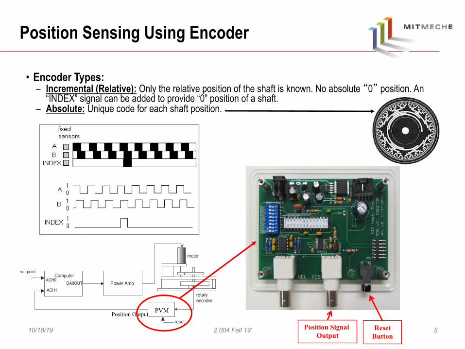
Position Sensing Using Encoder

• Encoder Types:– Incremental (Relative): Only the relative position of the shaft is known. No absolute “0” position. An

“INDEX” signal can be added to provide “0” position of a shaft.– Absolute: Unique code for each shaft position.

Reset Button

Position Signal Output

! " # $ % & ' ( )

( " * " %

+ $ * , ) " - . *

/ " ( ) 0 * $ %

' / 1 2

' / 1 3

4 ' 2 5 6 7

) " + - * - " . &

+ $ . + " %

8 4 ' / 9% " * : % ;

$ . < " = $ %

% $ + $ *

PVMPosition Output

10/18/19 2.004 Fall 19' 5

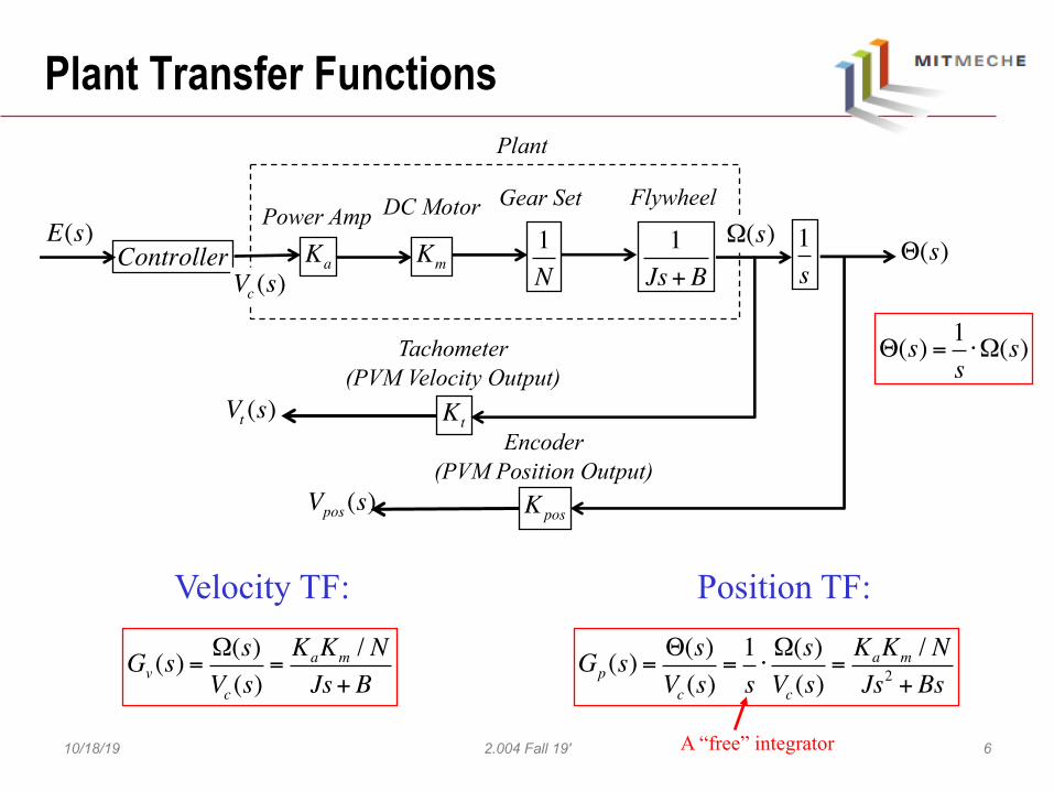
Plant Transfer Functions

Controller Ka Km1

Js+B1N

Kt

E(s)

Vt (s)

Power Amp DC Motor Gear Set Flywheel

Tachometer(PVM Velocity Output)

Plant

Ω(s)

Vc (s)

1s

Θ(s)

KposVpos (s)

Encoder(PVM Position Output)

Velocity TF:

Gv (s) =Ω(s)Vc (s)

=KaKm / NJs+B

Position TF:

Gp(s) =Θ(s)Vc (s)

=1s⋅Ω(s)Vc (s)

=KaKm / NJs2 +Bs

Θ(s) = 1s⋅Ω(s)

10/18/19 2.004 Fall 19' 6A “free” integrator

P, PI and PD Controllers

sKKsG i

pc +=)( sKKsG dpc +=)(

P Controller

pc KsG =)(

EncoderKpos

θ(t)

10/18/19 2.004 Fall 19' 7

Integral and Derivative

0 2 4 6 8 10 12 14 16 18 20Time (sec)

-2

-1.5

-1

-0.5

0

0.5

1

1.5

2

2.5

3

Ampl

itude

OriginalIntegralDerivativeLaggingLeading

10/18/19 2.004 Fall 19' 8

Original sine wave

Step Response and Its Derivative

0 2 4 6 8 10 12 14 16 18 20Time (sec)

-1

-0.5

0

0.5

1

1.5

2

Ampl

itude

Step responseDerivative of step response

Step response

Impulse response (derivative of step)

“Lead or anticipation effect”

10/18/19 2.004 Fall 19' 9

Comparison of Closed-Loop Transfer Functions

Gcl (s) =Vpos (s)R(s)

=KpKKpos

Js2 +Bs+KpKKpos

Gcl (s) =Vpos (s)R(s)

=Kp +Kds( )KKpos

Js2 + B+KdKKpos( )s+KpKKpos

K =KaKm

NLet

P Control:

PD Control:

22 2 nnss wzw ++

JB

n 2=Þzw

−Kp

KdA real zero at

10/18/19 2.004 Fall 19' 10

Settling time ±2%( ): Ts =4ζωn

2nd Order System Poles

TF(s) = Kdc ⋅ωn2

s2 + 2ζωns+ωn2 Tp =

π

ωn 1−ζ 2

Ts =4ζωn

±2%( )

%OS = e−

ζπ

1−ζ 2

"

#

$$

%

&

''×100

22,1 1 zwzwws -±-=±-= nndd jjs

02 22 =++ nnss wzw

10/18/19 2.004 Fall 19' 11

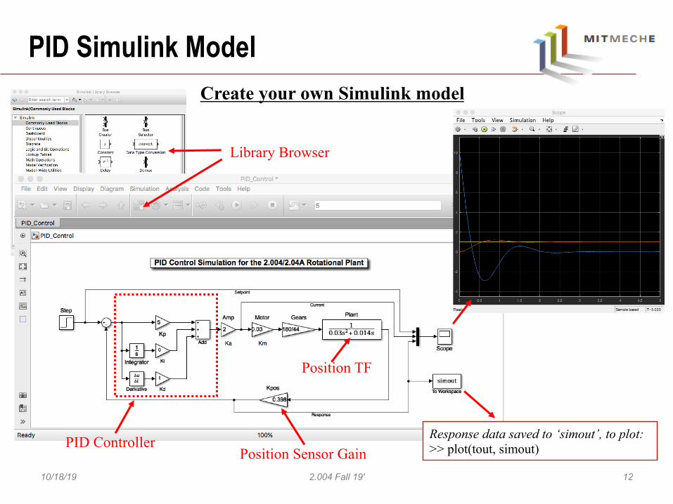
PID Simulink Model

PID Controller

Position TF

Position Sensor Gain10/18/19 2.004 Fall 19' 12

Create your own Simulink model

Library Browser

Response data saved to ‘simout’, to plot:>> plot(tout, simout)

Control Action Comparison

• Proportional action – improves speed but with steady-state error in some cases

• Integral action – improves steady state error but with less stability; may create overshoot, longer transient, or integrator windup

• Derivative action – improves stability but sensitive to noise; may create large output when the input is not a continuous signal

PID controller transfer function

10/18/19 2.004 Fall 19' 13

Gc (s) = Kp +Ki

s+Kds

=Kds

2 +Kps+Ki

s

= Kd

s2 + KpKd

⎛

⎝⎜

⎞

⎠⎟s+ Ki

Kd( )s

⎛

⎝

⎜⎜⎜⎜

⎞

⎠

⎟⎟⎟⎟

Practical Consideration

Band-limited differentiator to eliminate excess noise in the signal.

Finite difference method

10/18/19 2.004 Fall 19' 14

Use a Pseudo Differentiator

Practical Consideration

10/18/19 2.004 Fall 19' 15

0 0.2 0.4 0.6 0.8 1 1.2 1.4 1.6 1.8 2-0.5

0

0.5

1

1.5Smooth Step vs. Step Function

StepSmooth step

0 0.2 0.4 0.6 0.8 1 1.2 1.4 1.6 1.8 2Time (sec)

-0.5

0

0.5

1

1.5

2

2.5

3Derivative of Smooth Step Function

Use a Smooth Step Input

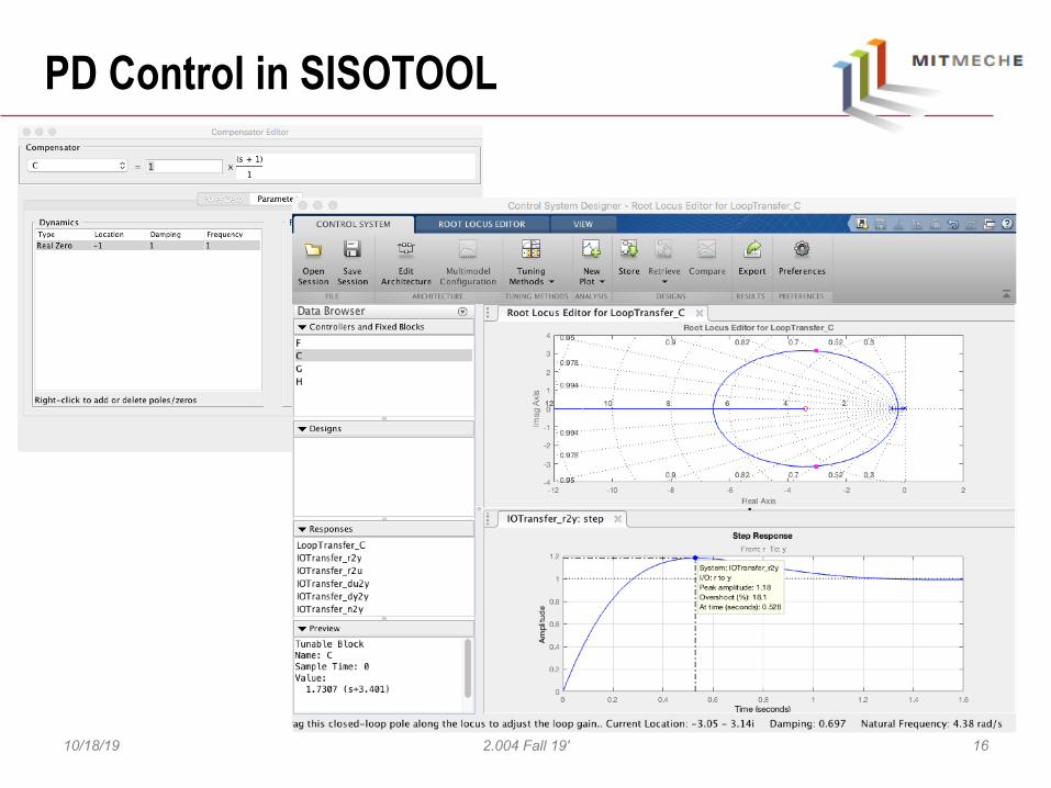
PD Control in SISOTOOL

10/18/19 2.004 Fall 19' 16

PD Control in SISOTOOL

10/18/19 2.004 Fall 19' 17

Kp 1+Kd

Kp

s⎛

⎝⎜⎜

⎞

⎠⎟⎟

KJs2 +Bs

Kpos

Vr (s)E(s)

Vpos (s)

+_ Θ(s)

Two open-loop poles:p1 = 0

p2 =−BJ

⎧

⎨⎪

⎩⎪

One open-loop zero: z =−Kp

Kd

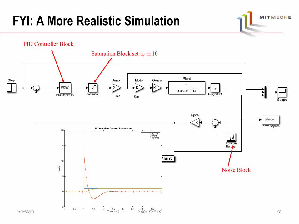
FYI: A More Realistic Simulation

10/18/19 2.004 Fall 19' 18

PID Controller Block

Saturation Block set to ±10

Time (sec)0 0.5 1 1.5 2 2.5 3 3.5 4 4.5 5

Volts

-5

0

5

10

15

20PD Position Control Simulation

Set pointCurrentResponse

Noise Block

Effect of Saturation

10/18/19 2.004 Fall 19' 19

Time (sec)0 0.5 1 1.5 2 2.5 3 3.5 4 4.5 5

Volts

0

0.2

0.4

0.6

0.8

1

1.2PD Position Control Step Response Simulation

With saturationWithout saturation

In control design, zeros play a major role

Effects of Zeros

• Zeroes reduce the effect of nearby poles• The derivative (lead) effect

10/18/19 2.004 Fall 19' 20

ï30 ï25 ï20 ï15 ï10 ï5 0 5ï10

ï8

ï6

ï4

ï2

0

2

4

6

8

100.30.520.70.820.90.95

0.978

0.994

0.30.520.70.820.90.95

0.978

0.994

510152025

Root Locus

Real Axis (secondsï1)

Imag

inar

y Ax

is (s

econ

dsï1

)

ï30 ï25 ï20 ï15 ï10 ï5 0 5ï10

ï8

ï6

ï4

ï2

0

2

4

6

8

100.30.520.70.820.90.95

0.978

0.994

0.30.520.70.820.90.95

0.978

0.994

510152025

Root Locus

Real Axis (secondsï1)

Imag

inar

y Ax

is (s

econ

dsï1

)

)10)(1(119)(1 ++

´=ss

sG)10)(1(

)11(9)(2 +++=ss

ssG

)()1()( 0 sGssG += aa1-=z

Step Response: )(1)(1)()1()( 000 sGs

sGs

sGssY aa +=+=

Impulse responseThe step response of )(0 sG

5.0=a

1=a

0<a

Step Response

zero initial slope

Impulse Response

hump

non-zero initial slope

22

2

0 2)(

nn

n

sssG

wzww

++=

For , the step response exhibits an undershoot. The output first moves in the opposite direction. The response is also very slow.

By adding the impulse response, i.e. the derivative of the step response, the resultant response becomes faster, but more overshoot.

0<a

Effects of Zeros

10/18/19 2.004 Fall 19' 21