JOINT DISTRIBUTIONS AND CORRELATION COEFFICIENTS

(Part 3)

2

TextbookShavelson, R.J. (1996). Statistical reasoning for the behavioral sciences (3rd Ed.). Boston: Allyn & Bacon.

Supplemental MaterialRuiz-Primo, M.A., Mitchell, M., & Shavelson, R.J. (1996). Student guide for Shavelson statistical reasoning for the behavioral sciences (3rd Ed.). Boston: Allyn & Bacon.

Textbook Credits

3

Overview

• Joint Distributions

• Correlation Coefficients

4

Joint Distributions and Correlation Coefficients • Correlational studies answer the question

- “What is the relationship of variable X and variable Y?”or - “How are scores on one measure (X) associated with scores on another measure(Y)?”

• First, we want to summarize the scores, and• Second, examine the relationship between the scores on the two measures

- First step: Arrange the scores to represent them in the form of a joint distribution (the representation of a pair of scores for each subject)

- Second step: Summarize the relationship represented by the JD with a single number we call correlation coefficient(a descriptive statistic that represents the magnitude of the relation, 0 to |1|, and the direction of the relation, + or -).

5

Research Example

The Psychological Belief Scale and Student Achievement

• Intuition and prior experience suggest that it is easier to learn from teachers who have the same beliefs as the students

• Prediction(intuition): - Students with similar beliefs as their instructors will earn the highest scores on exams- Exam scores should decrease as the difference in the students’ and instructors’ beliefs

increases• Study: 3 introductory Psych. classes at 3 different colleges with 7 students each, with

variable X representing a Belief Score and Y representing an Exam Score• What method to use?

- General: Combine the data and for all 3 classes examine one overall average X with Y?- More Specific: Examine X and Y in each class separately?

• Are the data consistent with predictions?

6

Research Example

The Psychological Belief Scale and Student Achievement

• Test 2 types of belief approaches: Humanistic(H) & Behavioristic(B)• Example: The central focus of the study of human behavior should be

- The specific principles that apply to unique individuals(H)- The general principles that apply to all individuals(B)

• Instructors and students received the belief scale beginning of course• Behavioristic orientation on the belief scale indicative by high scores• Humanistic orientation on the belief scale indicative by low scores

7

Joint Distribution: Tabular Representation• Behavioristic orientation on the belief scale indicative by high scores• Humanistic orientation on the belief scale indicative by low scores• Achievement(exam) score: students’ total scores earned in all class exams

8

Joint Distribution: Tabular Representation

Divided into 3 classes with 3 columns each. Take Class 1 as example:• Low belief scores are associated with moderately high exam scores(subjects 1 & 2)• Moderate belief scores are associated with high exam scores (subjects 3, 4, & 7)• High belief scores are associated with low exam scores (subjects 5 & 6)

9

Relationship of Student’s Belief & Exam Scores• Lines represent relationship between belief scale scores & exam scores• The magnitude of students’ scores differ from one class to the next as each instructor gave a different exam• So all exam scores were converted to standard scores showing how far above (+) or below (-) the class average a particular exam falls

10

Scatterplot of Student’s Belief & Exam Scores

A graphical representation of a JD showing pairs of each subject’s scores

11

Scatterplots for 3 classes & Instructor’s Belief Score

Comparison of Scatterplots for each of the 3 classes in the study

Curvilinear Relationship Curvilinear Relationship Linear Relationship

Suspect Outlier

12

Correlation Coefficients: Linear Relationships

13

Properties of Linear Correlation Coefficients

• The coefficient can take values from -1.00 to + 1.00 - A correlations of -0.95 indicates a very strong negative relationship between X & Y - A correlation of +0.95 indicates a very strong positive relationship between X & Y - A correlation of 0 indicates that there is no linear relationship between X & Y• The sign indicates the direction of the relationship between 2 variables• A positive relationship means: - Low scores on X go with low scores on Y - High scores on X go with high scores on Y(As X scores , Y scores ) • A negative relationship means: - Low scores on X go with high scores on Y - High scores on X go with low scores on Y(As X scores , Y scores )

14

Determining the Correlation Coefficient Magnitude

• Scatterplot characteristics are indicative of slope and data clustering: - Correlation is 0 if slope is horizontal & vertical slope is undefined - The clustering of data points determines the magnitude of correlation - Tight clustering means the magnitude of the correlation coefficient is high - Lose clustering means the magnitude of the correlation coefficient is low

15

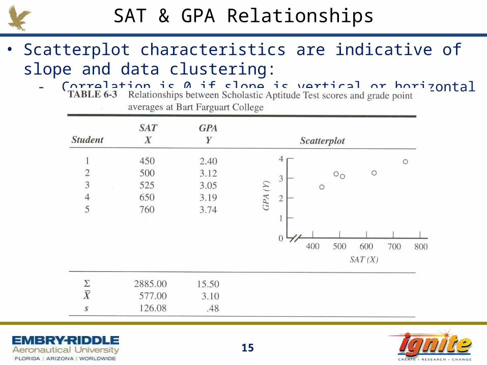
SAT & GPA Relationships

• Scatterplot characteristics are indicative of slope and data clustering: - Correlation is 0 if slope is vertical or horizontal

16

SAT & GPA Relationships

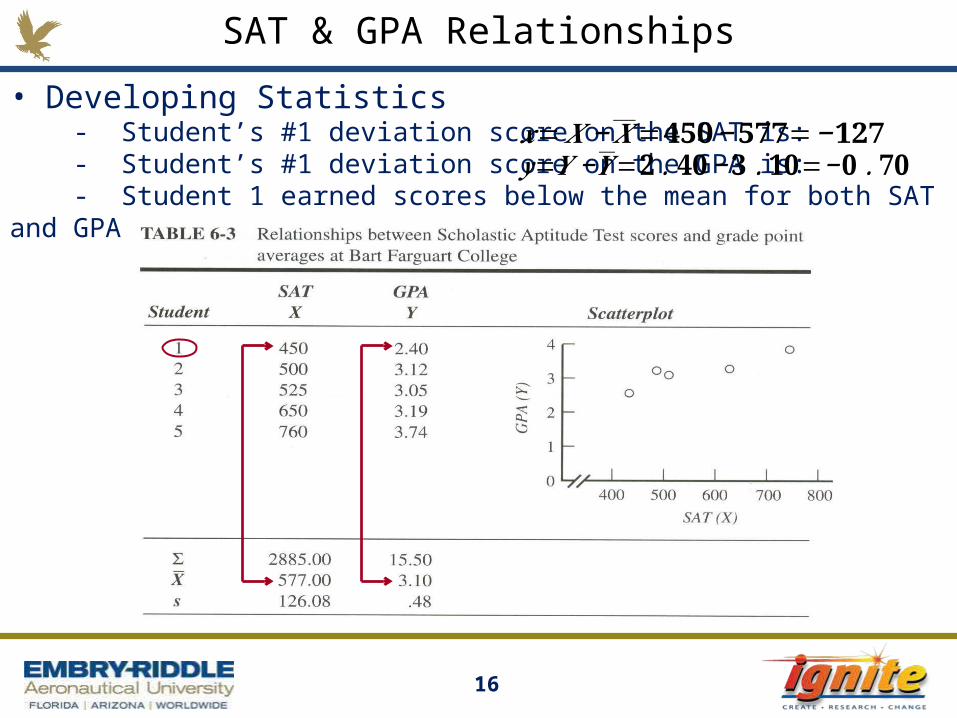
• Developing Statistics - Student’s #1 deviation score on the SAT is: - Student’s #1 deviation score on the GPA is: - Student 1 earned scores below the mean for both SAT and GPA

𝒙=𝑿−𝑿=𝟒𝟓𝟎−𝟓𝟕𝟕=−𝟏𝟐𝟕𝒚=𝒀 −𝒀=𝟐.𝟒𝟎−𝟑.𝟏𝟎=−𝟎 .𝟕𝟎

17

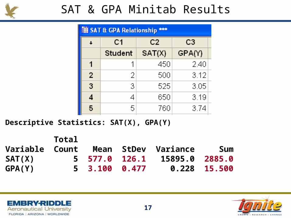
SAT & GPA Minitab Results

Descriptive Statistics: SAT(X), GPA(Y)

TotalVariable Count Mean StDev Variance SumSAT(X) 5 577.0 126.1 15895.0 2885.0GPA(Y) 5 3.100 0.477 0.228 15.500

18

Covariance of SAT & GPA Scores

• Measuring how two sets of deviation go together or covary - Student’s #1 covariance (cross product)is: - Note: When |x| and |y| are large xy is large (students 1 & 5) - Note: When |x| and |y| are small xy is small (students 2, 3, &4)

- Covariance:

- Pearson product-moment correlation coefficient measures the strength with X and Y

- Correlation coefficient:

𝑪𝒐𝒗 𝒙𝒚=∑ 𝒙𝒚𝑵−𝟏

=𝟐𝟏𝟑 .𝟔𝟓𝟒

=𝟓𝟑 .𝟒𝟏

𝒄𝒐𝒓𝒓𝒆𝒍𝒂𝒕𝒊𝒐𝒏 ( 𝑿 ,𝒀 )=𝒓 𝒙𝒚=𝑪𝒐𝒗 𝒙𝒚𝒔 𝒙 𝒔 𝒚

=𝟓𝟑 .𝟒𝟏

(𝟏𝟐𝟔 .𝟎𝟖) (𝟎 .𝟒𝟖)=𝟎 .𝟖𝟗

𝒙𝒚=(−𝟏𝟐𝟕) (−𝟎 .𝟕𝟎)=𝟖𝟖 .𝟗𝟎

19

Covariance of SAT & GPA Scores

• Measuring how two sets of deviation go together or covary - Student’s #1 covariance (cross product)is: - Note: When |x| and |y| are large xy is large (students 1 & 5) - Note: When |x| and |y| are small xy is small (students 2, 3, &4)

- Covariance:

- Pearson product-moment correlation coefficient measures the strength with X and Y

- Correlation coefficient:

𝒙𝒚=(−𝟏𝟐𝟕) (−𝟎 .𝟕𝟎)=𝟖𝟖 .𝟗𝟎

𝑪𝒐𝒗 𝒙𝒚=∑ 𝒙𝒚𝑵−𝟏

=𝟐𝟏𝟑 .𝟔𝟓𝟒

=𝟓𝟑 .𝟒𝟏

𝒄𝒐𝒓𝒓𝒆𝒍𝒂𝒕𝒊𝒐𝒏 ( 𝑿 ,𝒀 )=𝒓𝒙𝒚=𝑪𝒐𝒗 𝒙𝒚𝒔 𝒙 𝒔 𝒚

=𝟓𝟑 .𝟒𝟏

(𝟏𝟐𝟔 .𝟎𝟖 ) (𝟎 .𝟒𝟖 )=𝟎 .𝟖𝟗

Minitab Results

Covariances: SAT(X), GPA(Y)

SAT(X) GPA(Y)SAT(X) 15895.000GPA(Y) 53.413 0.228Correlations: SAT(X), GPA(Y)

Pearson correlation of SAT(X) and GPA(Y) = 0.888

20

Correlation Between SAT & GPA Scores

• Looking at the scatterplot to validate the correlation findings - A linear relationship with a positive slope indicates a positive correlation - The absolute magnitude 0.89 provides an index of the relationship strength(-1to +1) - Points cluster closely about an imaginary line validating the relationship magnitude

21

Minitab Output: SAT & GPA Scores

• Looking at the scatterplot to validate the correlation findings - A linear relationship with a positive slope indicates a positive correlation - The absolute magnitude 0.89 provides an index of the relationship strength(-1to +1) - Points cluster closely about an imaginary line validating the relationship magnitude

22

Excel Output: SAT & GPA Scores

SAT (X) GPA (Y)

Mean 577 Mean 3.1Standard Error 56.38262144 Standard Error 0.2133776Median 525 Median 3.12Mode #N/A Mode #N/AStandard Deviation 126.0753743 Standard Deviation 0.477126818Sample Variance 15895 Sample Variance 0.22765Kurtosis -0.813601983 Kurtosis 1.83955472Skewness 0.805065221 Skewness -0.307822135Range 310 Range 1.34Minimum 450 Minimum 2.4Maximum 760 Maximum 3.74Sum 2885 Sum 15.5Count 5 Count 5

23

Excel Output SAT & GPA Scores

24

The Squared Correlation Coefficient

• The squared correlation coefficient is the coefficient of determination - It is the amount of variability that can be explained between X & Y• Recall: The larger |rxy| is, the stronger the relationship between X & Y

• We previously found that:

• So

• Now we want to convert to percentage of variance - Tells us the percentage that X shares with Y in terms of variability to one another - The % of variance in Y and X that can be explained is:

𝒓 𝒙𝒚=𝑪𝒐𝒗 𝒙𝒚𝒔 𝒙 𝒔 𝒚

=𝟓𝟑 .𝟒𝟏

(𝟏𝟐𝟔 .𝟎𝟖) (𝟎 .𝟒𝟖)=𝟎 .𝟖𝟗

𝒓𝟐 𝒙𝒚=𝟎 .𝟖𝟗𝟐=𝟎.𝟕𝟗𝟐𝟏

𝒓𝟐 𝒙𝒚×𝟏𝟎𝟎=𝟎 .𝟕𝟗𝟐𝟏×𝟏𝟎𝟎=𝟕𝟗 .𝟐𝟏%

25

Percentage of Variance

• Pictorial representation of the % of variance in exam scores accounted for by the variability in belief scores (computed from class 3 data)

Variability in X Variability in Y

26

Spearman Rank Correlation Coefficient

• Non-linear (curvilinear) monotonic increasing or decreasing functions

Monotonically decreasing f Monotonically increasing f

27

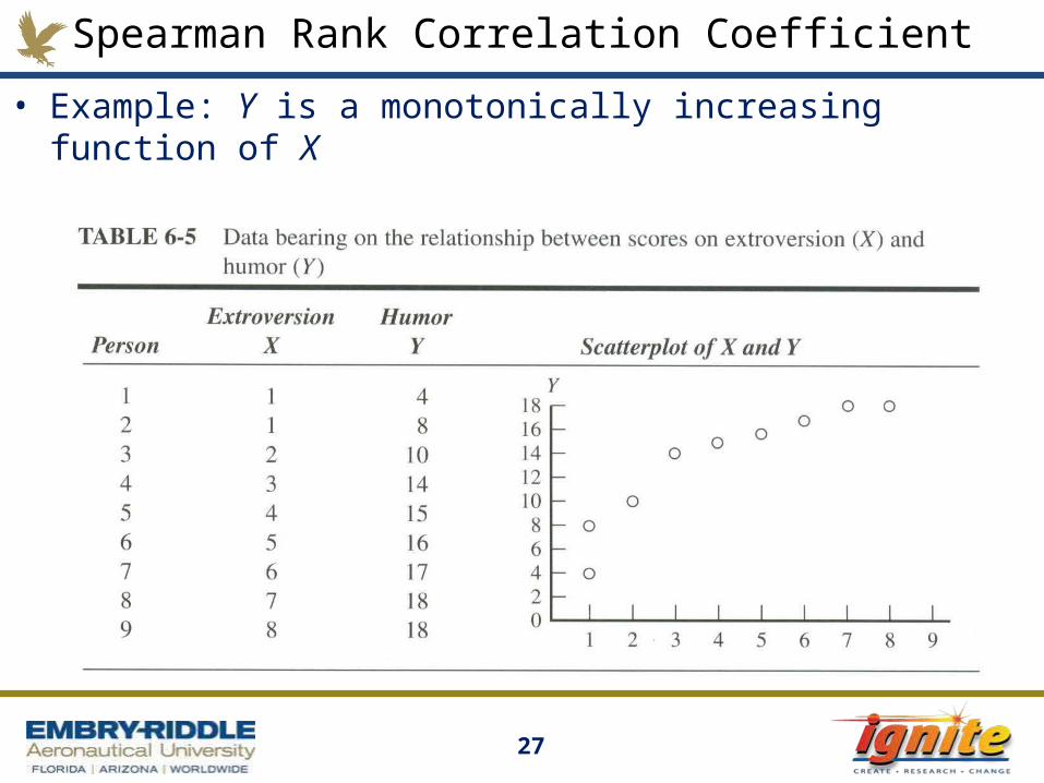
Spearman Rank Correlation Coefficient

• Example: Y is a monotonically increasing function of X

28

Spearman Rank Correlation Coefficient

• Rank ordering the data for both X & Y and graph - The converted ordered graph is now linear - We can now compute the Pearson correlation coefficient for ranks between X & Y

29

Spearman Rank Correlation Coefficient

30

Sources of Misleading Correlation Coefficients

• Too much confidence can lead to misleading interpretations - Restriction of the range of values on one of the variables may reduce the magnitude of the correlation coefficient

31

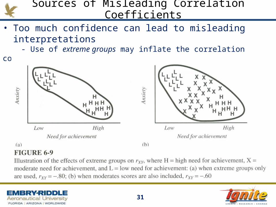
Sources of Misleading Correlation Coefficients

• Too much confidence can lead to misleading interpretations - Use of extreme groups may inflate the correlation coefficient

32

Sources of Misleading Correlation Coefficients

• Too much confidence can lead to misleading interpretations - Combining groups with different means on one or both variables may have an unpredictable effect on the correlation coefficient

33

Sources of Misleading Correlation Coefficients

• Too much confidence can lead to misleading interpretations - Extreme scores (Outliers) may have a marked effect on the correlation coefficient, especially if the sample size is small

34

Sources of Misleading Correlation Coefficients

• Too much confidence can lead to misleading interpretations - A curvilinear relationship between X and Y may account for a near-zero correlation coefficient

No systematic relationship Curvilinearly related: Use the eta (h) ratio coefficient measurement instead of the Pearson correlation coefficient

35

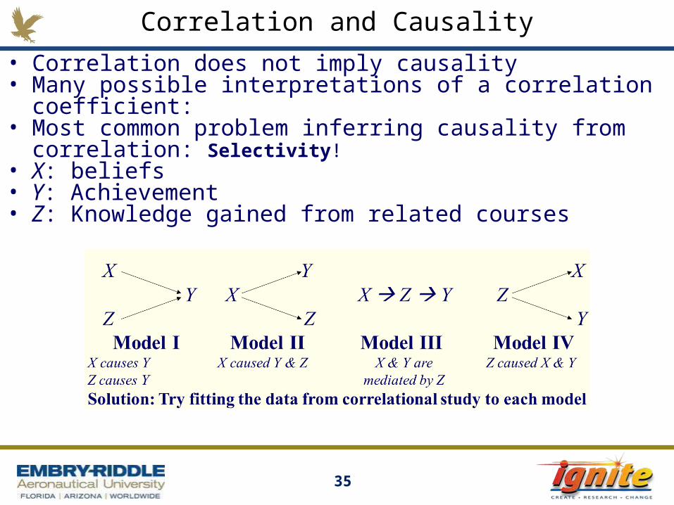
Correlation and Causality• Correlation does not imply causality• Many possible interpretations of a correlation coefficient:• Most common problem inferring causality from correlation: Selectivity!• X: beliefs• Y: Achievement• Z: Knowledge gained from related courses

36

Practice ExercisesPart 2 Practice Exercises1. Select a hypothetical product or a process and create some test data of your choice

(plausible, no more than 10) as shown in textbook/class2. Show your type of experimental approach3. Create a detailed table of frequency distributions4. Display your data with different types of graphs5. Calculate the measures of central tendency and variability6. Calculate the Z-score(s) and indicate the relative position in the normal distribution.7. Provide any other pertinent information as a result

Part 3 Practice Exercises8. Represent your joint distribution data in a tabular form9. Create a scatterplot of your data10. Create a covariance table (as table 6-4) and calculate the

covariance11. Calculate the correlation of the two variables12. Calculate the R squared value and explain your findings as a result

37

Comments/Questions ?