2 road vehicle modeling - maxwell
TRANSCRIPT
2Road vehicle modeling
2.1Simple handling model
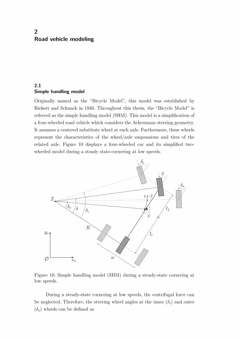
Originally named as the “Bicycle Model”, this model was established byRiekert and Schunck in 1940. Throughout this thesis, the “Bicycle Model” isrefereed as the simple handling model (SHM). This model is a simplification ofa four-wheeled road vehicle which considers the Ackermann steering geometry.It assumes a centered substitute wheel at each axle. Furthermore, these wheelsrepresent the characteristics of the wheel/axle suspensions and tires of therelated axle. Figure 10 displays a four-wheeled car and its simplified two-wheeled model during a steady state-cornering at low speeds.
ψ
δi
δo
δ
w
lf
lr
vI β
δo δ δi
R
O xo
yo
Figure 10: Simple handling model (SHM) during a steady-state cornering atlow speeds.
During a steady-state cornering at low speeds, the centrifugal force canbe neglected. Therefore, the steering wheel angles at the inner (δi) and outer(δo) wheels can be defined as
Chapter 2. Road vehicle modeling 37
tan(δi) = l
R − w/2 and tan(δo) = l
R + w/2 , (2-1)
where R is the radius of curvature of the rear substitute wheel around theinstantaneous center of rotation (I); l = lf + lr is also know as the vehicle’swheel-base and w its track-width. Then, rearranging the Equation (2-1), it ispossible to define the Ackermann steering geometry via
cot(δo) − cot(δi) = w
l. (2-2)
This Ackermann condition is fulfilled only for small speeds. However, in mostcases, cars will perform a curve at considerable speeds. Therefore, the deviationΔδ = δa
o − δAo , obtained by the difference between the actual steering wheel
angle δao and the one computed using the Equation (2-2), i.e. δA
o , is used as aquality indicator of the steering system of commercial vehicles. Finally, it isalso possible to calculate the steering wheel angle of the SHM (δ) via
tan(δ) = l
Ror cot(δ) = cot(δo) + cot(δi)
2 . (2-3)
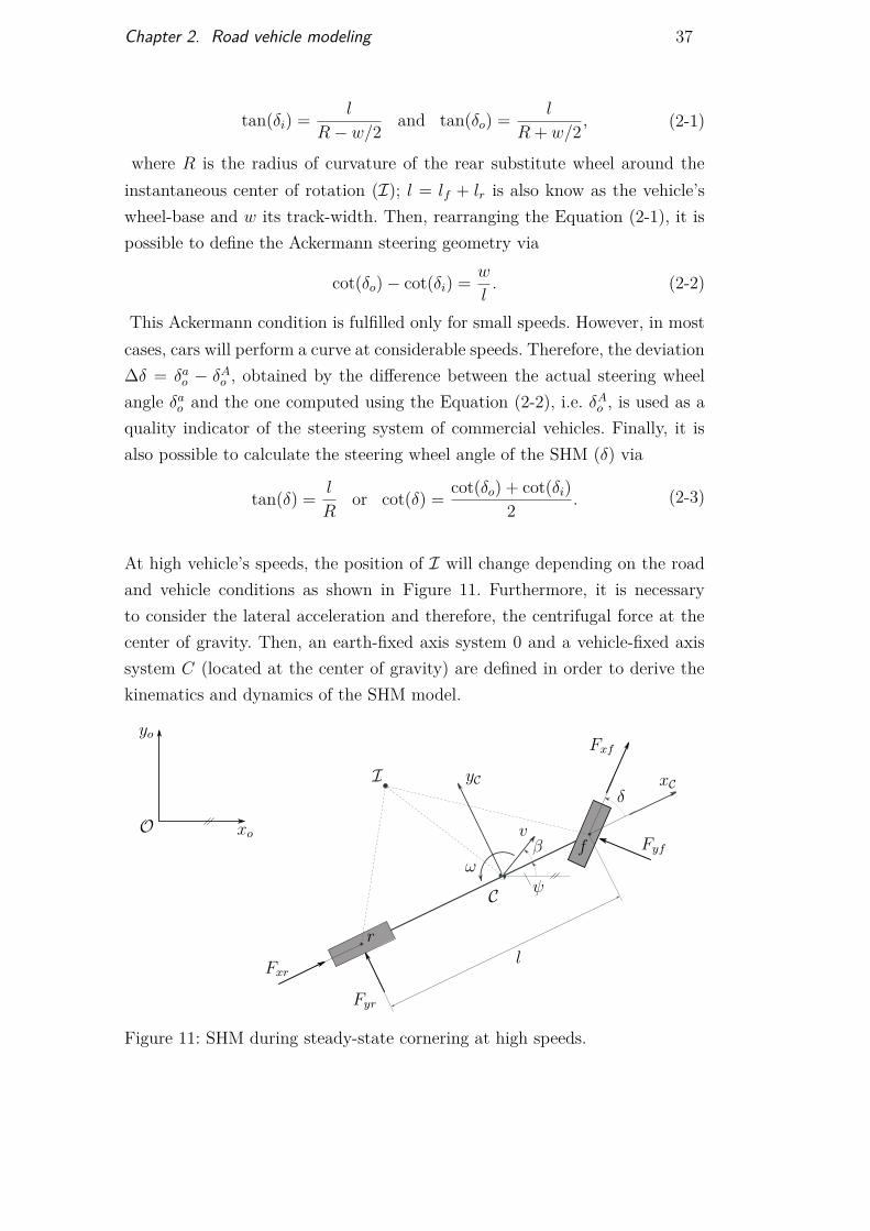
At high vehicle’s speeds, the position of I will change depending on the roadand vehicle conditions as shown in Figure 11. Furthermore, it is necessaryto consider the lateral acceleration and therefore, the centrifugal force at thecenter of gravity. Then, an earth-fixed axis system 0 and a vehicle-fixed axissystem C (located at the center of gravity) are defined in order to derive thekinematics and dynamics of the SHM model.
Oδ
l
ψ
β
Fxr
Fyr
Fxf
Fyf
xo
yo
C
xCyCI
v
r
fω
Figure 11: SHM during steady-state cornering at high speeds.
Chapter 2. Road vehicle modeling 38
2.1.1Kinematics
Using the axis systems defined before, see Figure 11, the velocity and theangular velocity of the SHM expressed in C are obtained via
v0i,C =
v cos β
v sin β
0
and ω0C,C =
00ψ
, (2-4)
where β is the sideslip angle measured at the the center of gravity C and ψ
is the yaw angular velocity of the SHM model. Additionally, the contact pointvelocities at each centered wheel are calculated via
v0j,C = v0j,C + ω0C,C × rCj,C , (2-5)
where j = {f, r} represents the contact point of the front and rear centeredwheel respectively and, rCi,C is its position vector expressed in C. Finally,using the Equations (2-4) and (2-5), the contact points velocities are obtainedas follows
v0f,C =
v cos β
v sin β + ψlf
0
and v0r,C =
v cos β
v sin β − ψlr
0
. (2-6)
This contact point velocities are needed to compute the degree of slip,specifically the lateral tire slip, of each substitute centered wheel of the SHM.
2.1.2Equations of motion
In order to derive the equations of motion, the acceleration of the SHM needto be derived. In this model, it is assumed small sideslip angles, i.e. β � 1 andconsequently, the Equation (2-4) can be simplified to
v0i,C =
v
|v|β0
, (2-7)
and the Equation ((2-6)) to
v0f,C =
v
|v|β + ψlf
0
and v0r,C =
v
|v|β − ψlr
0
. (2-8)
Then, doing the time derivation of Equation (2-7), the acceleration is com-
Chapter 2. Road vehicle modeling 39
puted as
a0C,C = v0C,C + ω0C,C × v0i,C =
0vψ + |v|β
0
(2-9)
where the constant speed v = 0 was assumed and higher order terms wereomitted. Also the angular acceleration of the SHM is obtained via
α0C,C = ω0C,C =
00ψ
. (2-10)
Lateral tire forces
As mentioned before, the lateral acceleration must be considered duringsteady-state cornering at high speeds. Thus, the centrifugal force should becompensated by lateral forces, generated by the deformation of the contactpatch see Figure 7, at the substitute tires in order to perform a curve.Therefore, small lateral sliding motions occur at the tire contact points (f, r)and in consequence, it can be assumed that the tires operate in its linear region.Then, it is possible to compute the lateral forces at each centered wheel via
Fyf = Kfsyf and Fyr = Krsyr, (2-11)
where syf and syr represent the lateral slips at the front and rear contactpoints respectively; Kf and Kr represent the cornering stiffness of the frontand rear axle. In addition, even if the tires are equal, Kf and Kr could bedifferent due to its dependency of wheel load and also of the suspension config-uration. Therefore, computing the correct cornering stiffness brings a properSHM model and in consequence, a correct analysis of the lateral dynamics, atlow lateral accelerations, can be realized.
Lateral tire slips
The lateral tire slip sy is defined as
sy = − vty
|rDΩ| , (2-12)
where vty represent the lateral tire velocity, rD is the static tire radius and Ωis the wheel angular velocity. Moreover, the SHM model is not accelerating ordecelerating. Therefore, the wheels are in a rolling condition, i.e. rDΩ = vtx,where vtx is the longitudinal tire velocity. In addition, the components vtx
and vty can be computed projecting the contact point velocity into the tirelongitudinal and lateral axis respectively via
Chapter 2. Road vehicle modeling 40
vtx = eTtxvi,C and vty = eT
tyvi,C , (2-13)
where vi,C represents the contact point velocity that are defined in Equa-tion (2-8); etx and ety are the tire longitudinal and lateral unit vectors re-spectively, and are calculated for the front and rear substitute tires as follows
front: etx =
cos δ
sin δ
0
, ety =
− sin δ
cos δ
0
rear: etx =
100
, ety =
010
(2-14)
Finally, using Equations (2-8), (2-12), (2-13) and (2-14), we obtain the lateralslip of the front centered wheel, syf , via
syf = v sin δ − cos δ(|v|β + lf ψ)|v cos δ + sin δ(|v|β + lf ψ)| ,
and also, the lateral slip syr of the rear centered wheel as
syr = − |v|β − lrψ
|v|
then, assuming small steering wheel angles δ < 0.2 and also, small yaw angularvelocities ψ, i.e. |lf ψ| � |v| and |lrψ| � |v|, the lateral slips were reduced to
syf = −β − lf|v| ψ + v
|v|δ and syr = −β + lr|v| ψ . (2-15)
Finally, the equations of motion of the SHM model are described by its lateraldynamics, i.e in the y-axis, via
m�vψ + |v|β
�= Fyf + Fyr, (2-16)
and also with its yaw rate dynamics, i.e. around the z-axis, as
Θψ = lfFyf − lrFyr, (2-17)
where m and Θ represents the mass and the moment of inertia (z-axis)of the SHM respectively. Finally, considering the linear tire model definedby Equation (2-11) and the lateral slips defined by Equation (2-15), in theequations of motion (2-16) and (2-17) were obtained
Chapter 2. Road vehicle modeling 41
β = Kf
m|v|
�−β − lf
|v| ψ + v
|v|δ�
+ Kr
m|v|
�−β + lr
|v| ψ�
− v
|v| ψ
ψ = lfKf
Θ
�−β − lf
|v| ψ + v
|v|δ�
− lrKr
Θ
�−β + lr
|v| ψ�
.
(2-18)
In addition, these equations can be represented by a space-state equation asfollows
β
ψ
=
−Kf + Kr
m|v|lrKr − lfKf
m|v||v| − v
|v|lrKr − lfKf
Θ − l2fKf + l2
rKr
Θ|v|
β
ψ
+
v
|v|Kf
m|v|v
|v|lfKf
Θ
δ
� �� � � �� � � �� � � �� � � �� �x = A x + B u
(2-19)
This formulation, Equation (2-19), can be used for stability, phase-planeanalysis as well as for design of safety control systems, e.g. ESP and activefront steering systems (AFS). In addition, this model can easily be extendedfor all-wheel steering vehicles, i.e. including rear wheel steering. In fact, thisextended model is employed to design control strategies for four-wheel steeringsystems (4WS). This variant of the simple handling vehicle model is presentedin Chapter 4.
The planar vehicle model presented above was derived taking intoaccount several assumptions and simplifications. However, for advance vehicledynamic applications, a fully non-linear and three-dimensional vehicle model isneeded. This model should consider the nonlinearities of the main componentsthat affects the behavior of passenger cars. In the followings subsections,modeling aspects of road vehicles and its subsystems are described.
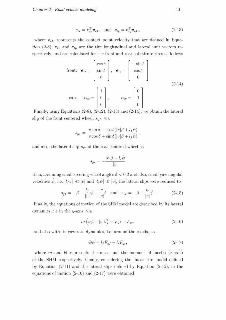
2.2Multibody vehicle model
In general, road vehicles are modeled by multibody systems [17, 33]. Thisis a common approach for the study of the vehicle’s handling [47] and rideproperties [48, 49], and also for the design of vehicle safety systems [45, 46].The overall multibody vehicle model can be divided in different systems, e.g.the vehicle framework, steering, the power drive-train, the road and the tire,see Figure 12. The vehicle framework includes the vehicle’s body or chassis andmodules for the wheel/axle suspension system. In addition, external loads, the
Chapter 2. Road vehicle modeling 42
engine and the driver/passengers can be included on the vehicle framework.For handling and ride analysis of passenger cars, the chassis can be modeledas a rigid body. However, in heavy trucks models, the chassis compliance andthe driver’s cabin should be considered.
Tire
Road
Steeringsystem
WheelSuspension system
Vehicleframework
EngineDriver Passenger
Load
Drive-train
Figure 12: Multibody road vehicle model, tire and road system [33].
Besides the vehicle’s framework, i.e. vehicle body, wheel/axle suspensionsystem, steering system and power drive-train, the tire-road interaction playsan essential role in road vehicles. In fact, this interaction generates thenecessary forces to move the car. In the next subsections, a modeling aspectof the wheel/axle suspension, tire and road system is presented.
2.2.1Modeling considerations
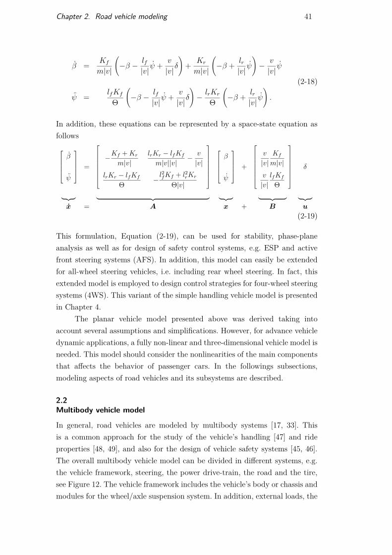
In this thesis, nine rigid bodies are employed to model the road vehicledynamics, i.e. one chassis, four knuckles and four wheels (tire + rim). Inaddition, some reference axis systems are also defined to describe the motionof the bodies. In Figure 13, the rigid bodies and their axis systems as wellas the earth-fixed axis system with origin O are illustrated. The vehicle axissystem V , located at the middle of the front axle, is defined by ISO Standard8855, i.e. with positive xV in the forward direction, positive yV to the driver’sleft and positive zV up. In addition, each wheel-fixed axis system is located atthe geometric center of its respective knuckle.
Chapter 2. Road vehicle modeling 43
In total, this multibody vehicle model has 14 degrees of freedom (DOF).The DOF include the vehicle’s body translations {xV , yV , zV }; the vehicle’sbody rotations {α, β, γ}; the wheels’ vertical displacements {z1, z2, z3, z4} aswell as their spin speeds {ω1, ω2, ω3, ω4}. Furthermore, the subscripts {1,2,3,4}indicate the front left, front right, rear left and rear right wheels respectively.
ω3
ω1
ω2
ω4
wheel
knuckle
z1
z2
z3
z4
bodyV
Ox
z
y
earth-fixedaxis system
vehicle-fixedaxis system
yV
zV γ
β
αxV
wheel-fixedaxis system
W
Figure 13: Degrees of freedom (DOF) of the multibody road vehicle model.Graphic representation modified from [33].
2.2.2Suspension system
The suspension is one of the most important mechanical subsystems in roadvehicles. This system connects each wheel’s body to the chassis throughmechanical and force elements. Some functionalities of the suspension systeminvolves:
– carry the vehicle’s weight,
– maintain a correct wheel alignment,
– ensure a good contact between the tire and the road,
– reduce the effect of road impacts.
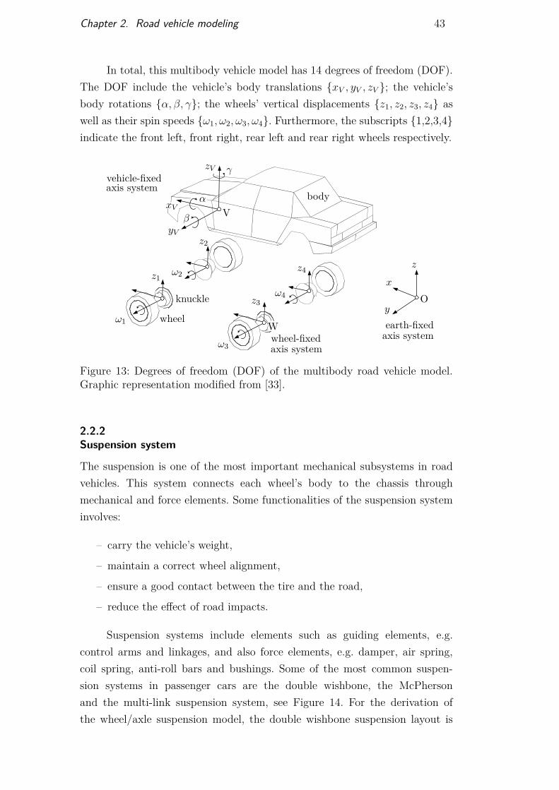
Suspension systems include elements such as guiding elements, e.g.control arms and linkages, and also force elements, e.g. damper, air spring,coil spring, anti-roll bars and bushings. Some of the most common suspen-sion systems in passenger cars are the double wishbone, the McPhersonand the multi-link suspension system, see Figure 14. For the derivation ofthe wheel/axle suspension model, the double wishbone suspension layout is
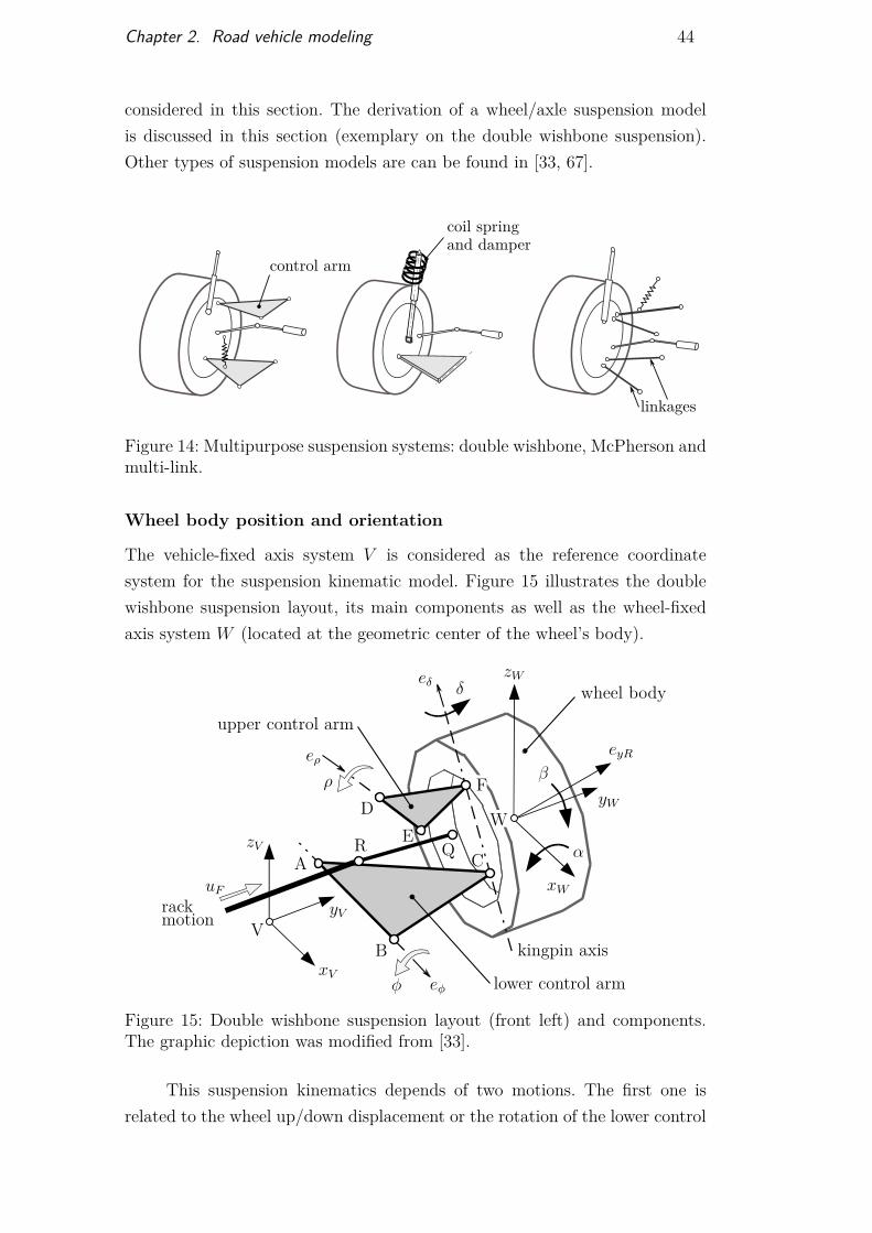
Chapter 2. Road vehicle modeling 44
considered in this section. The derivation of a wheel/axle suspension modelis discussed in this section (exemplary on the double wishbone suspension).Other types of suspension models are can be found in [33, 67].
control arm
coil springand damper
linkages
Figure 14: Multipurpose suspension systems: double wishbone, McPherson andmulti-link.
Wheel body position and orientation
The vehicle-fixed axis system V is considered as the reference coordinatesystem for the suspension kinematic model. Figure 15 illustrates the doublewishbone suspension layout, its main components as well as the wheel-fixedaxis system W (located at the geometric center of the wheel’s body).
V
δ
uF
xV
yV
zV
φ
eyR
W
xW
yW
zW
rackmotion
ρ
A
B
C
DE
F
R Q
eφ
eδ
α
β
kingpin axis
lower control arm
upper control arm
eρ
wheel body
Figure 15: Double wishbone suspension layout (front left) and components.The graphic depiction was modified from [33].
This suspension kinematics depends of two motions. The first one isrelated to the wheel up/down displacement or the rotation of the lower control
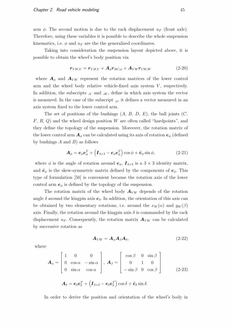
Chapter 2. Road vehicle modeling 45
arm φ. The second motion is due to the rack displacement uF (front axle).Therefore, using these variables it is possible to describe the whole suspensionkinematics, i.e. φ and uF are the the generalized coordinates.
Taking into consideration the suspension layout depicted above, it ispossible to obtain the wheel’s body position via
rV W,V = rV B,V + AφrBC,φ + AV W rCW,W (2-20)
where Aφ and AV W represent the rotation matrices of the lower controlarm and the wheel body relative vehicle-fixed axis system V , respectively.In addition, the subscripts ,V and ,W , define in which axis system the vectoris measured. In the case of the subscript ,φ, it defines a vector measured in anaxis system fixed to the lower control arm.
The set of positions of the bushings (A, B, D, E), the ball joints (C,F , R, Q) and the wheel design position W are often called “hardpoints”, andthey define the topology of the suspension. Moreover, the rotation matrix ofthe lower control arm Aφ can be calculated using its axis of rotation eφ (definedby bushings A and B) as follows
Aφ = eφeTφ +
�I3×3 − eφeT
φ
�cos φ + �eφ sin φ, (2-21)
where φ is the angle of rotation around eφ, I3×3 is a 3 × 3 identity matrix,and �eφ is the skew-symmetric matrix defined by the components of eφ. Thistype of formulation [50] is convenient because the rotation axis of the lowercontrol arm eφ is defined by the topology of the suspension.
The rotation matrix of the wheel body AV W depends of the rotationangle δ around the kingpin axis eδ. In addition, the orientation of this axis canbe obtained by two elementary rotations, i.e. around the xW (α) and yW (β)axis. Finally, the rotation around the kingpin axis δ is commanded by the rackdisplacement uF . Consequently, the rotation matrix AV W can be calculatedby successive rotation as
AV W = AαAβAδ, (2-22)where
Aα =
1 0 00 cos α − sin α
0 sin α cos α
, Aβ =
cos β 0 sin β
0 1 0− sin β 0 cos β
Aδ = eδeTδ +
�I3×3 − eδe
Tδ
�cos δ + �eδ sin δ.
(2-23)
In order to derive the position and orientation of the wheel’s body in
Chapter 2. Road vehicle modeling 46
function of the generalized coordinates, i.e. φ and uF , kinematic constraintsneed to be considered.
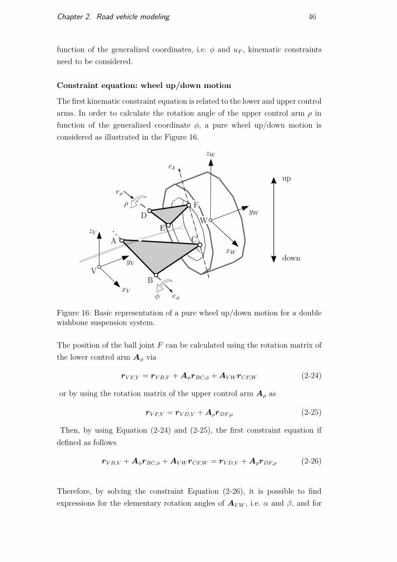
Constraint equation: wheel up/down motion
The first kinematic constraint equation is related to the lower and upper controlarms. In order to calculate the rotation angle of the upper control arm ρ infunction of the generalized coordinate φ, a pure wheel up/down motion isconsidered as illustrated in the Figure 16.
V
xV
yV
zV
φ
W
xW
yW
zW
ρ
A
B
C
DE
F
eφ
eδ
eρ
up
down
Figure 16: Basic representation of a pure wheel up/down motion for a doublewishbone suspension system.
The position of the ball joint F can be calculated using the rotation matrix ofthe lower control arm Aφ via
rV F,V = rV B,V + AφrBC,φ + AV W rCF,W (2-24)
or by using the rotation matrix of the upper control arm Aρ as
rV F,V = rV D,V + AρrDF,ρ (2-25)
Then, by using Equation (2-24) and (2-25), the first constraint equation ifdefined as follows
rV B,V + AφrBC,φ + AV W rCF,W = rV D,V + AρrDF,ρ (2-26)
Therefore, by solving the constraint Equation (2-26), it is possible to findexpressions for the elementary rotation angles of AV W , i.e. α and β, and for
Chapter 2. Road vehicle modeling 47
the rotation of the upper control arm ρ in terms of φ. These expression can bewritten as follows
α = α(φ), β = β(φ) and ρ = ρ(φ) (2-27)
As consequence of the previous equation, the elementary rotation matrices canbe written as
Aα = Aα(φ) and Aβ = Aβ(φ). (2-28)
In addition, the rotation matrix Aδ depends of eδ and the orientation of thisaxis depends of φ, therefore, Aδ = Aδ(φ). Finally, Equation (2-22) can berewritten as function of φ, i.e. for pure wheel up/down motions, as
AV W = Aα(φ)Aβ(φ)Aδ(φ) (2-29)
and consequently, the position of the wheel’s body relative to the vehicle-fixedaxis system V (Equation (2-20)) is also function of φ. Details about thederivation of the expressions α = α(φ), β = β(φ) and ρ = ρ(φ) can be foundin Appendix A.1.
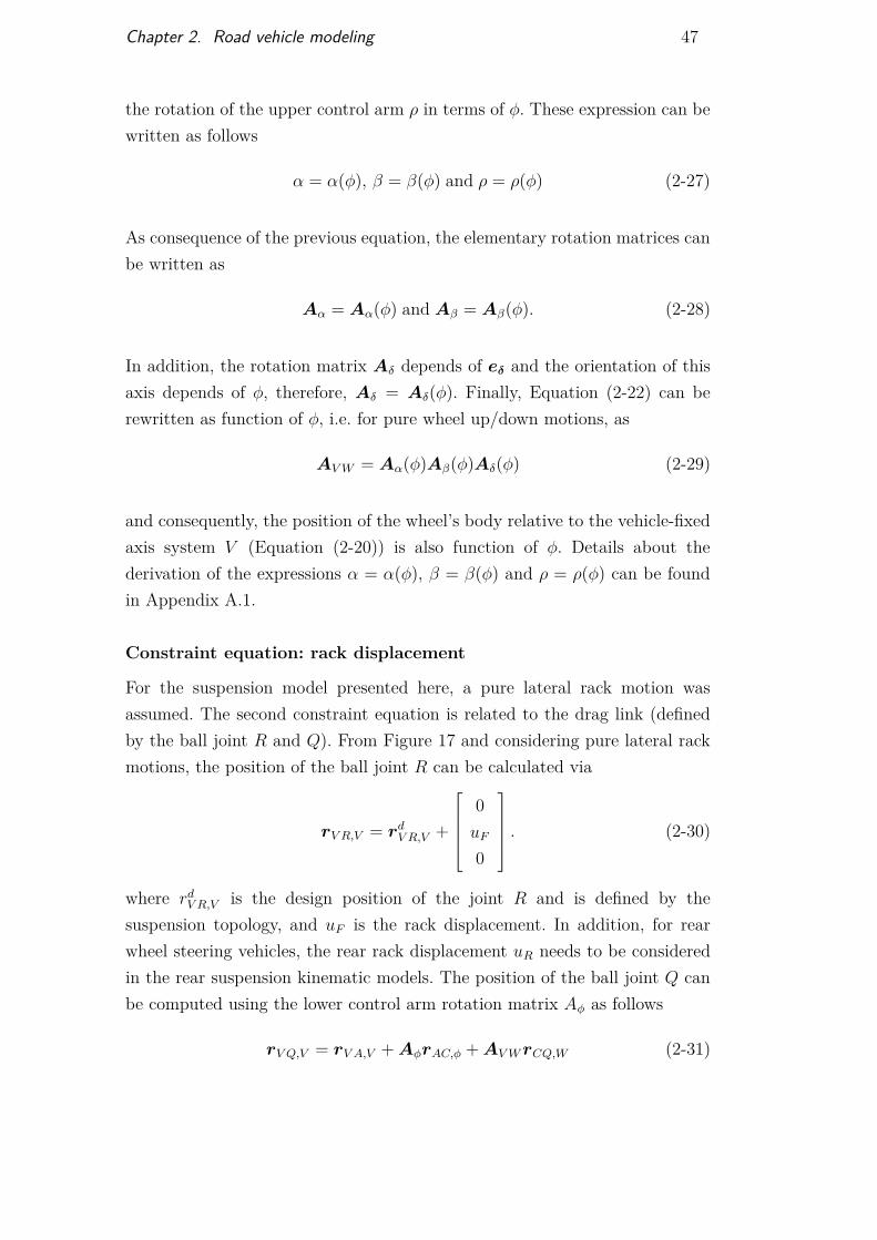
Constraint equation: rack displacement
For the suspension model presented here, a pure lateral rack motion wasassumed. The second constraint equation is related to the drag link (definedby the ball joint R and Q). From Figure 17 and considering pure lateral rackmotions, the position of the ball joint R can be calculated via
rV R,V = rdV R,V +
0uF
0
. (2-30)
where rdV R,V is the design position of the joint R and is defined by the
suspension topology, and uF is the rack displacement. In addition, for rearwheel steering vehicles, the rear rack displacement uR needs to be consideredin the rear suspension kinematic models. The position of the ball joint Q canbe computed using the lower control arm rotation matrix Aφ as follows
rV Q,V = rV A,V + AφrAC,φ + AV W rCQ,W (2-31)
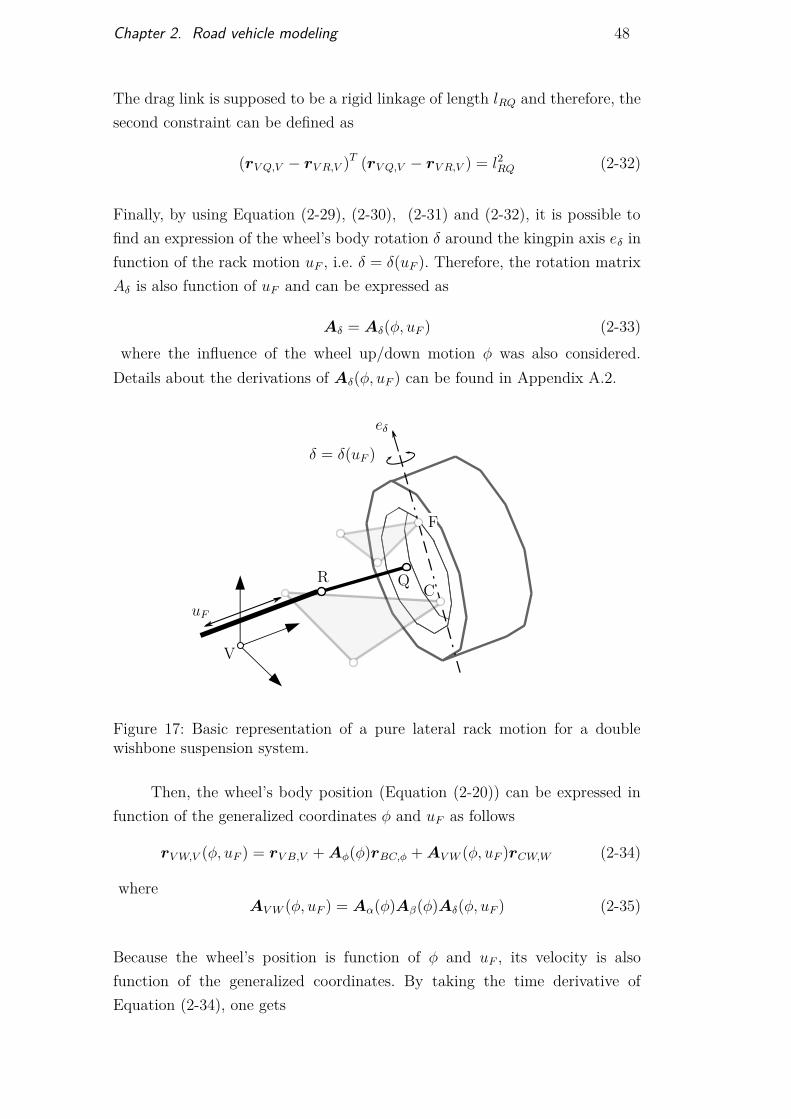
Chapter 2. Road vehicle modeling 48
The drag link is supposed to be a rigid linkage of length lRQ and therefore, thesecond constraint can be defined as
(rV Q,V − rV R,V )T (rV Q,V − rV R,V ) = l2RQ (2-32)
Finally, by using Equation (2-29), (2-30), (2-31) and (2-32), it is possible tofind an expression of the wheel’s body rotation δ around the kingpin axis eδ infunction of the rack motion uF , i.e. δ = δ(uF ). Therefore, the rotation matrixAδ is also function of uF and can be expressed as
Aδ = Aδ(φ, uF ) (2-33)where the influence of the wheel up/down motion φ was also considered.
Details about the derivations of Aδ(φ, uF ) can be found in Appendix A.2.
V
δ = δ(uF )
uF
C
F
R Q
eδ
Figure 17: Basic representation of a pure lateral rack motion for a doublewishbone suspension system.
Then, the wheel’s body position (Equation (2-20)) can be expressed infunction of the generalized coordinates φ and uF as follows
rV W,V (φ, uF ) = rV B,V + Aφ(φ)rBC,φ + AV W (φ, uF )rCW,W (2-34)
whereAV W (φ, uF ) = Aα(φ)Aβ(φ)Aδ(φ, uF ) (2-35)
Because the wheel’s position is function of φ and uF , its velocity is alsofunction of the generalized coordinates. By taking the time derivative ofEquation (2-34), one gets
Chapter 2. Road vehicle modeling 49
rV W,V (φ, uF ) = ∂rV W,V
∂φφ + ∂rV W,V
∂uF
uF (2-36)
On the order hand, the wheel’s body angular velocity can be calculated via
ωV W (φ, uF ) = ∂ωV W
∂φφ + ∂ωV W
∂uF
uF (2-37)
A physical interpretation of the partial derivatives of the wheel’s body velocityand angular velocity respect to the generalized speeds, i.e. φ and uF , presentedin Equation (2-36) and (2-37) could be, how the tire forces (generated inthe tire-road contact area) are transfered to the vehicle’s body through thesuspension system.
Following the same modeling process presented above, it is possibleto model complex suspension systems like multi-link or even a Formula 1suspension concept, e.g. push-rod and pull-rod suspension systems.
2.2.3Tire modeling
The tires are complex and essential elements in road vehicles. They areresponsible to transmit the engine power to the road and consequently,generate the necessary forces to move the car, e.g. accelerate/braking thevehicle or negotiate a curve. These forces are created in the contact patch, i.e.the contact area between the tire and the road surface. In the current literature,there are two main approaches for tire modeling, i.e. empirical and physical.The first approach uses mathematical functions to fit experimental tire forcecurves [54]. In spite of matching these data extremely well, these tire models donot offer a physical meaning of its empirical parameters. In the other hand, tiremodels based on finite element methods are physical models that are employedcommonly for high frequency analysis, e.g. vehicle comfort simulations underuneven roads. These tire models are computer time consuming and need a largenumber of experimental data. Consequently, they are too complicated to beused in vehicle handling simulations. However, a simplification of these typesof models can make them suitable for multibody vehicle applications [51].
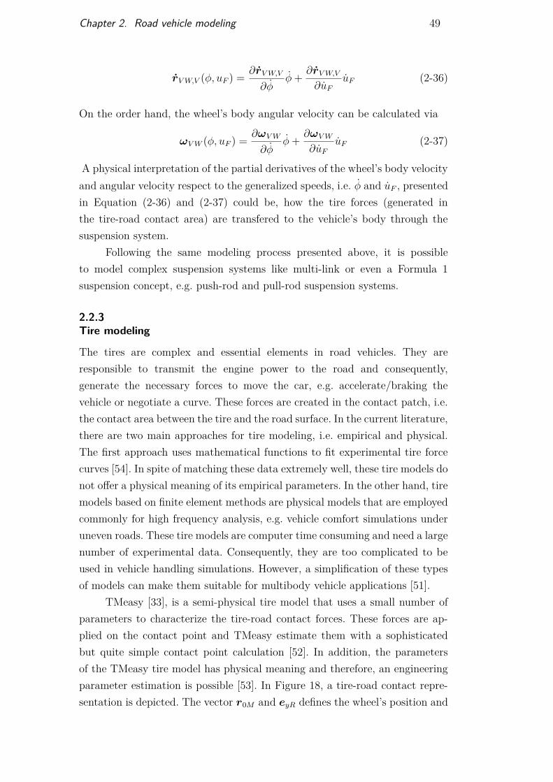
TMeasy [33], is a semi-physical tire model that uses a small number ofparameters to characterize the tire-road contact forces. These forces are ap-plied on the contact point and TMeasy estimate them with a sophisticatedbut quite simple contact point calculation [52]. In addition, the parametersof the TMeasy tire model has physical meaning and therefore, an engineeringparameter estimation is possible [53]. In Figure 18, a tire-road contact repre-sentation is depicted. The vector r0M and eyR defines the wheel’s position and
Chapter 2. Road vehicle modeling 50
orientation in relation to the earth-fixed axis system. In addition, the localroad plane z = z(x, y) can be defined by a road point P0 and a unit vectorperpendicular to this plane en, as can be seen in the right side of Figure 18.
tire
eyR
z = z(x, y) local road plane
rimcenterplane
γ
wheelcarrier
ex
ey
ab
P
rMP
x0
y0
z0
0
eyR
en
ezR
MM
P0
r0M
Figure 18: TMeasy contact point and local plane geometry [53].
The longitudinal, lateral and radial tire directions can be computed via
ex = eyR × en
|eyR × en| , ey = en × ex and ezR = ex × eyR, (2-38)
respectively. Moreover, ex was normalized because eyR is not perpendicular(in general) to the road normal vector en. This deviation is defined by thetire camber angle γ and then, a first but quite realistic approximation of thecontact point P is obtained by
rMP,0 = −rSezR, (2-39)
where rS is the static tire radius and ezR was defined in Equation (2-38). Moredetails about the contact point calculation can be found in [52].
In normal driving maneuvers, e.g. acceleration or deceleration in a curve,the longitudinal slip sx and lateral slip sy occur at the same time. Therefore, thecombination of slips and thus of the longitudinal and lateral forces should behandled by the tire model. In order to achieve the contribution of longitudinaland lateral slips to the combined slip, with a similar weight, TMeasy performsa normalization process as follows:
s =
�����
sx
sx
�2+�
sy
sy
�2
=�
(sNx )2 +
�sN
y
�2(2-40)
where sNx and sN
y are the normalized slips. Furthermore, the normalizing fac-tors sx and sy take into account the longitudinal and lateral force characteris-tics and are defined via
Chapter 2. Road vehicle modeling 51
si = sMi
sMx + sM
y
+ F Mi /dF 0
i
F Mx /dF 0
x + F My /dF 0
y
, i = {x, y}. (2-41)
Similar to the curve of longitudinal and lateral forces, the combined forceF = F (s) can be defined by their characteristic parameters dF 0, sM , F M , sS,and F S. These parameters are defined as:
dF 0 =�
(dF 0x sx cos φ)2 + (dF 0
y sy sin φ)2
sM =��
sMx
sxcos φ
�2+�
sMy
sysin φ
�2
F M =�
(F Mx cos φ)2 +
�F M
y sin φ�2
sS =��
sSx
sxcos φ
�2+�
sSy
sysin φ
�2
F S =�
(F Sx cos φ)2 +
�F S
y sin φ�2
.
(2-42)
The angular function φ is used to grant a smooth transition from thelongitudinal and lateral force to the combined force. Finally, the longitudinaland lateral resulting forces are derived from the combined force as follows:
Fx = F cos(φ), Fy = F sin(φ) where cos(φ) = sNx
s, sin(φ) =
sNy
s. (2-43)
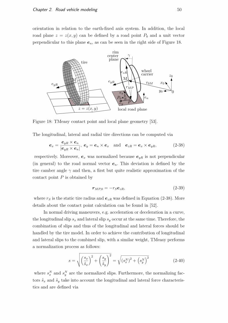
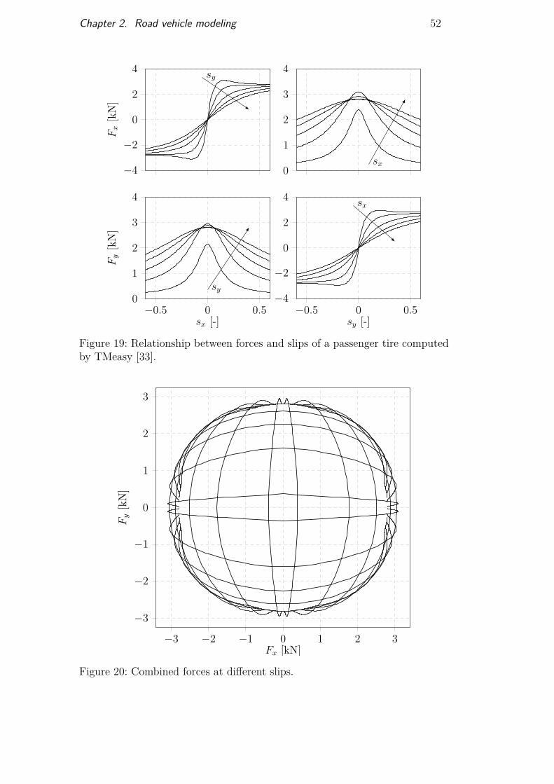
Figure 19 shows the mutual influence of longitudinal and lateral forcesagainst the longitudinal and lateral slips, computed by TMeasy, for a standardcommercial tire. Details of the tire characteristics are presented in Table 1.
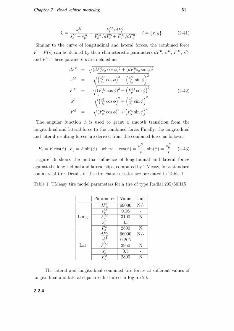
Table 1: TMeasy tire model parameters for a tire of type Radial 205/50R15
Parameter Value Unit
Long.
dF 0x 69000 N/-
sMx 0.16 -
F Mx 3100 N
sSx 0.5 -
F Sx 2800 N
Lat.
dF 0y 66000 N/-
sMy 0.205 -
F My 2950 N
sSx 0.5 -
F Sy 2800 N
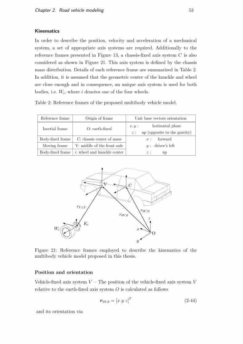
The lateral and longitudinal combined tire forces at different values oflongitudinal and lateral slips are illustrated in Figure 20.
2.2.4
Chapter 2. Road vehicle modeling 52
Figure 19: Relationship between forces and slips of a passenger tire computedby TMeasy [33].
Figure 20: Combined forces at different slips.
Chapter 2. Road vehicle modeling 53
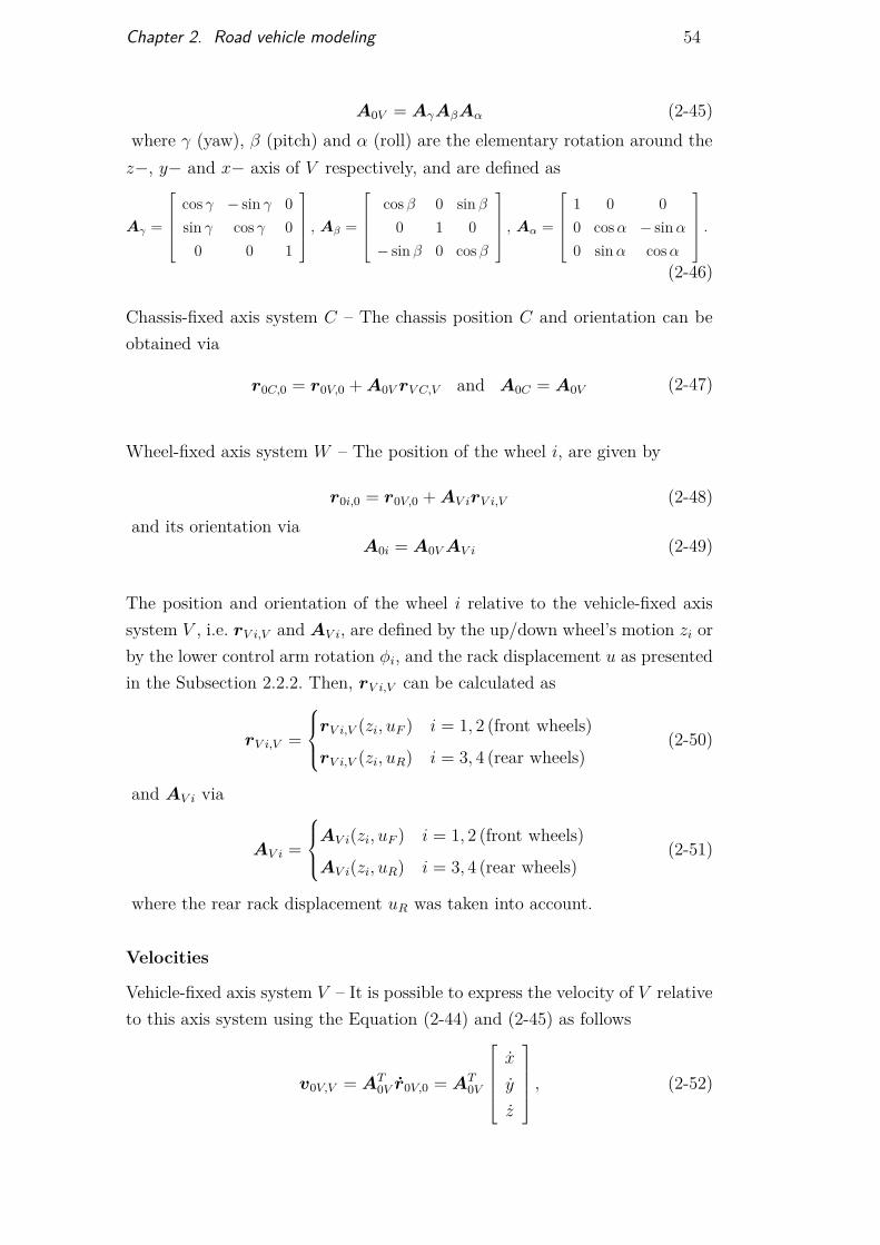
Kinematics
In order to describe the position, velocity and acceleration of a mechanicalsystem, a set of appropriate axis systems are required. Additionally to thereference frames presented in Figure 13, a chassis-fixed axis system C is alsoconsidered as shown in Figure 21. This axis system is defined by the chassismass distribution. Details of each reference frame are summarized in Table 2.In addition, it is assumed that the geometric center of the knuckle and wheelare close enough and in consequence, an unique axis system is used for bothbodies, i.e. Wi, where i denotes one of the four wheels.
Table 2: Reference frames of the proposed multibody vehicle model.
Reference frame Origin of frame Unit base vectors orientation
Inertial frame O: earth-fixedx, y : horizontal planez : up (opposite to the gravity)
Body-fixed frame C: chassis center of mass x : forwardy : driver’s leftz : up
Moving frame V: middle of the front axleBody-fixed frame i: wheel and knuckle center
Ox
z
y
V C
r0V,0
rV i,Vr0C,0
Wi
Ki
i
Figure 21: Reference frames employed to describe the kinematics of themultibody vehicle model proposed in this thesis.
Position and orientation
Vehicle-fixed axis system V – The position of the vehicle-fixed axis system V
relative to the earth-fixed axis system O is calculated as follows
r0V,0 = [x y z]T (2-44)
and its orientation via
Chapter 2. Road vehicle modeling 54
A0V = AγAβAα (2-45)where γ (yaw), β (pitch) and α (roll) are the elementary rotation around the
z−, y− and x− axis of V respectively, and are defined as
Aγ =
cos γ − sin γ 0sin γ cos γ 0
0 0 1
, Aβ =
cos β 0 sin β
0 1 0− sin β 0 cos β
, Aα =
1 0 00 cos α − sin α
0 sin α cos α
.
(2-46)
Chassis-fixed axis system C – The chassis position C and orientation can beobtained via
r0C,0 = r0V,0 + A0V rV C,V and A0C = A0V (2-47)
Wheel-fixed axis system W – The position of the wheel i, are given by
r0i,0 = r0V,0 + AV irV i,V (2-48)and its orientation via
A0i = A0V AV i (2-49)
The position and orientation of the wheel i relative to the vehicle-fixed axissystem V , i.e. rV i,V and AV i, are defined by the up/down wheel’s motion zi orby the lower control arm rotation φi, and the rack displacement u as presentedin the Subsection 2.2.2. Then, rV i,V can be calculated as
rV i,V =
rV i,V (zi, uF ) i = 1, 2 (front wheels)
rV i,V (zi, uR) i = 3, 4 (rear wheels)(2-50)
and AV i via
AV i =
AV i(zi, uF ) i = 1, 2 (front wheels)
AV i(zi, uR) i = 3, 4 (rear wheels)(2-51)
where the rear rack displacement uR was taken into account.
Velocities
Vehicle-fixed axis system V – It is possible to express the velocity of V relativeto this axis system using the Equation (2-44) and (2-45) as follows
v0V,V = AT0V r0V,0 = AT
0V
x
y
z
, (2-52)
Chapter 2. Road vehicle modeling 55
and its angular velocity can be decomposed in elementary velocities via
ω0V,V =
100
α +
0cos α
− sin α
β +
− sin β
sin α cos β
cos α cos β
γ
=
1 0 − sin β
0 cos α sin α cos β
0 − sin α cos α cos β
α
β
γ
.
(2-53)
Using the vehicle-fixed axis system V to derive the velocities and accelerationsof the bodies is quite convenient because, for example, a simplification is pos-sible by employing the components of v0V,V and ω0V,V as generalized speeds.Furthermore, the suspension kinematics was already defined relative to thisaxis system, then the velocity and acceleration of the wheel’s body can beobtained easily.
Chassis-fixed axis system C – the velocity of C relative to V is obtainedderiving Equation (2-47) via
r0C,0 = r0V,0 + A0V rV C,V + A0V rV C,V , (2-54)
then by left-multiplication with AT0V , i.e. transformation in the vehicle-fixed
axis system V , results in
v0C,V = v0V,V + ω0V,V × rV C,V , (2-55)
where rV C,V = 0 (constant in V ) and the equivalences AT0V A0V = �ω0V,V and
�ωr = ω × r were take into account. In addition, the chassis-fixed axis systemC angular velocity is simply given by ω0C,V = ω0V,V .
Wheel-fixed axis system Wi – The velocity of a specific wheel’s body i relativeto O can be calculated by time derivative of Equation (2-48) as follows
r0i,0 = r0V,0 + A0V rV i,V + A0V rV i,V , (2-56)
then by left-multiplication with AT0V results in
v0i,V = v0V,V + ω0V,V × rV i,V + rV i,V , (2-57)
where rV i,V is defined by the suspension kinematic model presented in Sub-section 2.2.2. In addition, the time derivative of rV i,V , provided by Equa-tion (2-50), results in
Chapter 2. Road vehicle modeling 56
rV i,V = ∂rV i,V
∂zi
zi + ∂rV i,V
∂u∗u∗ = tiz zi + tiu∗ u∗ (2-58)
where tiz and tiu∗ represents the partial velocities of the wheel-i relative tozi and u∗ respectively, and u∗ = uF for i = 1, 2 (front rack displacement)and u∗ = uR for i = 3, 4 (rear rack displacement). In addition, the wheel’sorientation is defined by the knuckle’s orientation because both of them areattached to the same reference frame W . Therefore, the angular velocity of theknuckle relative to the vehicle-fixed axis system V can be obtained as
ω0Ki,V = ω0V,V + ωV i,V , (2-59)
and ωV i,V , similarly to the wheel’s body position rV i,V , can be expressed asfollows
ωV i,V = diz zi + diu∗u∗ (2-60)where diz and diu∗ are the partial angular velocities of the knuckle and u∗
follows the same rule as presented before. Finally, the absolute angular velocityof the wheel-i is given by
ω0Wi,V = ω0V,V + ωV i,V + AV ieyRi,iϕi (2-61)
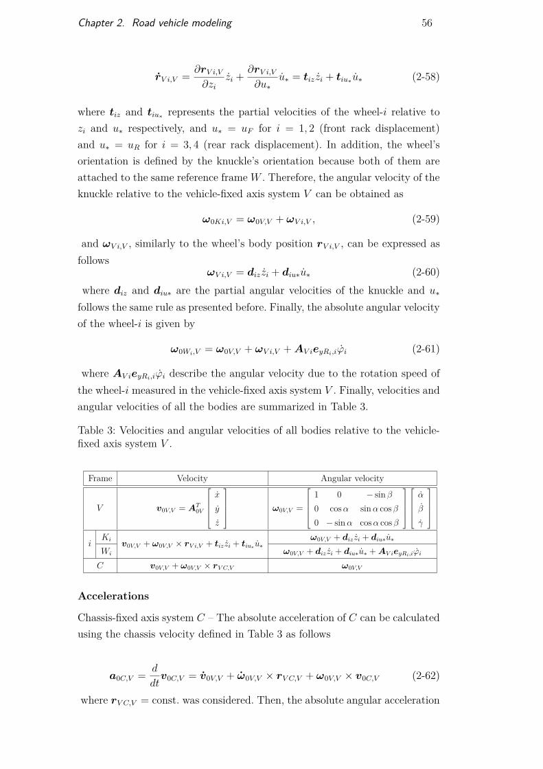
where AV ieyRi,iϕi describe the angular velocity due to the rotation speed ofthe wheel-i measured in the vehicle-fixed axis system V . Finally, velocities andangular velocities of all the bodies are summarized in Table 3.
Table 3: Velocities and angular velocities of all bodies relative to the vehicle-fixed axis system V .
Frame Velocity Angular velocity
V v0V,V = AT0V
x
y
z
ω0V,V =
1 0 − sin β
0 cos α sin α cos β
0 − sin α cos α cos β
α
β
γ
iKi
v0V,V + ω0V,V × rV i,V + tiz zi + tiu∗ u∗ω0V,V + diz zi + diu∗u∗
Wi ω0V,V + diz zi + diu∗u∗ + AV ieyRi,iϕi
C v0V,V + ω0V,V × rV C,V ω0V,V
Accelerations
Chassis-fixed axis system C – The absolute acceleration of C can be calculatedusing the chassis velocity defined in Table 3 as follows
a0C,V = d
dtv0C,V = v0V,V + ω0V,V × rV C,V + ω0V,V × v0C,V (2-62)
where rV C,V = const. was considered. Then, the absolute angular acceleration
Chapter 2. Road vehicle modeling 57
is obtained via
α0C,V = d
dtω0C,V = ω0V,V + ω0V,V × ω0C,V (2-63)
where because ω0C,V = ω0V,V their cross-product is equal to zero and there-fore, α0C,V = ω0V,V .
Wheel body-fixed axis system i – The acceleration of the wheel body-i relativeto V can be calculated by the derivation of its velocity shown in Table 3 asfollows
a0i,V = d
dtv0i,V = v0V,V + ω0V,V × rV i,V + tiz zi + tiu∗u∗
+ ω0V,V × rV i,V + tiz zi + tiu∗ u∗ + ω0V,V × v0i,V
(2-64)
Using the information of the angular velocities shown in Table 3, it is possibleto express the absolute angular acceleration of the knuckle-i via
α0Ki,V = d
dtω0Ki,V = ω0V,V + diz zi + diu∗u∗
+ diz zi + diu∗ u∗ + ω0V,V × ω0Ki,V
(2-65)
and the absolute angular acceleration of the wheel-i is given by
α0Wi,V = d
dtω0Wi,V = ω0V,V + diz zi + diu∗u∗ + AV ieyRi,iϕi
+ diz zi + diu∗ u∗ + ωV i,V × AV ieyRi,iϕi + ω0V,V × ω0Wi,V
(2-66)
2.2.5Equations of motion
With the velocities and accelerations of all the bodies of the multibody vehiclemodel already defined then, it is necessary a method to derive the equationsof motion of the system.
The Jourdain’s principle
As written in [68], the Jourdain’s principle (1908) states:A constrained mechanical systems performs motions such that the totalvirtual power of the constraint forces and torques δP c is zero.
For a multibody system of k rigid bodies, the Jourdain’s principle can beapplied as follows
δP c =k�
i=1
�δvT
i F ci + δωT
i T ci
�= 0 (2-67)
Chapter 2. Road vehicle modeling 58
The virtual velocities δvi and δωi are arbitrary and infinitesimal variationsof the velocity and angular velocity of the body i. In addition, these virtualvelocities are completely compatible with the constraint at any time and atany position, and are defined via
δvi = ∂vi
∂zδz and δωi = ∂ωi
∂zδz (2-68)
where z is a vector that collects the generalized speeds. Furthermore, thetranslational motion of a rigid body i is governed by Newton’s law as
mia0i = F ai + F c
i (2-69)
and the rotational motion by Euler equation via
Θiα0i + ω0i × Θiω0i = T ai + T c
i (2-70)where the total force and torque were divided in the applied and
constraint forces and torques respectively. Then, by employing equa-tions (2-67), (2-68), (2-69) and (2-70), it is possible to obtain the equations ofmotion of the mechanical system as follows
K(q) q = z, M(q) z = g(q, z) (2-71)
where M(q) is know as the mass matrix and is given by
M(q) =k�
i=1
�∂vT
0i
∂zmi
∂v0i
∂z+ ∂ωT
0i
∂zΘi
∂ω0i
∂z
�(2-72)
and g(q, z) is the vector of generalized forces and torques and is defined via
g(q, z) =k�
i=1
�∂vT
0i
∂z(F a
i − miaR0i) + ∂ωT
0i
∂z(T a
i − ΘiαR0i − ω0i × Θiω0i)
�
(2-73)and
q = [x, y, z, α, β, γ, z1, z2, uF , z3, z4, uR, ϕ1, ϕ2, ϕ3, ϕ4] (2-74)where q is a vector that collects the generalized coordinates of the vehicle,
K is the kinematic matrix used to define an appropriate vector of generalizedspeeds z, i.e.
z = [vx0V , vy
0V , vz0V , ωx
0V , ωy0V , ωz
0V , z1, z2, uF , z3, z4, uR, ω1, ω2, ω3, ω4]. (2-75)
where [vx0V , vy
0V , vz0V ] and [ωx
0V , ωy0V , ωz
0V ] are the components of v0V,V andω0V,V , see Table 3, and ωi = ϕi is the spin speed of the wheel-i. Furthermore,the partial velocities ∂vT
0i
∂zand partial angular velocities ∂ωT
0i
∂zcan be calculated
using information from Table 3 and the vector of generalized speeds defined in
Chapter 2. Road vehicle modeling 59
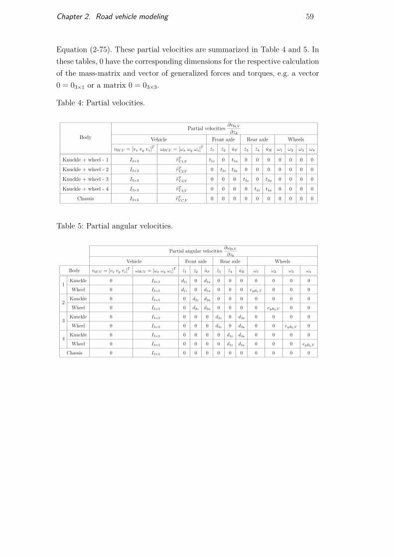
Equation (2-75). These partial velocities are summarized in Table 4 and 5. Inthese tables, 0 have the corresponding dimensions for the respective calculationof the mass-matrix and vector of generalized forces and torques, e.g. a vector0 = 03×1 or a matrix 0 = 03×3.
Table 4: Partial velocities.
BodyPartial velocities ∂v0i,V
∂zk
Vehicle Front axle Rear axle Wheels
v0V,V = [vx vy vz]T ω0V,V = [ωx ωy ωz]T z1 z2 uF z3 z4 uR ω1 ω2 ω3 ω4
Knuckle + wheel - 1 I3×3 �rTV 1,V t1z 0 t1u 0 0 0 0 0 0 0
Knuckle + wheel - 2 I3×3 �rTV 2,V 0 t2z t2u 0 0 0 0 0 0 0
Knuckle + wheel - 3 I3×3 �rTV 3,V 0 0 0 t3z 0 t3u 0 0 0 0
Knuckle + wheel - 4 I3×3 �rTV 4,V 0 0 0 0 t4z t4u 0 0 0 0
Chassis I3×3 �rTV C,V 0 0 0 0 0 0 0 0 0 0
Table 5: Partial angular velocities.
Partial angular velocities ∂ω0i,V
∂zk
Vehicle Front axle Rear axle Wheels
Body v0V,V = [vx vy vz]T ω0V,V = [ωx ωy ωz]T z1 z2 uF z3 z4 uR ω1 ω2 ω3 ω4
1Knuckle 0 I3×3 d1z 0 d1u 0 0 0 0 0 0 0
Wheel 0 I3×3 d1z 0 d1u 0 0 0 eyR1,V 0 0 0
2Knuckle 0 I3×3 0 d2z d2u 0 0 0 0 0 0 0
Wheel 0 I3×3 0 d2z d2u 0 0 0 0 eyR2,V 0 0
3Knuckle 0 I3×3 0 0 0 d3z 0 d3u 0 0 0 0
Wheel 0 I3×3 0 0 0 d3z 0 d3u 0 0 eyR3,V 0
4Knuckle 0 I3×3 0 0 0 0 d4z d4u 0 0 0 0
Wheel 0 I3×3 0 0 0 0 d4z d4u 0 0 0 eyR4,V
Chassis 0 I3×3 0 0 0 0 0 0 0 0 0 0