2. government association number 3. … · venky shankar and samer madanat 8. ... in the case of...

1. REPORT NUMBER CA15-2317

2. GOVERNMENT ASSOCIATION NUMBER 3. RECIPIENT'S CATALOG NUMBER

4. TITLE AND SUBTITLE

METHODS FOR IDENTIFYING HIGH COLLISION CONCENTRATIONS FOR IDENTIFYING POTENTIAL SAFETY IMPROVEMENTS: DEVELOPMENT OF SAFETY PERFORMANCE FUNCTIONS FOR CALIFORNIA

5. REPORT DATE January 31, 2015 6. PERFORMING ORGANIZATION CODE

7. AUTHOR Venky Shankar and Samer Madanat

8. PERFORMING ORGANIZATION REPORT NO.

9. PERFORMING ORGANIZATION NAME AND ADDRESS Institute of Transportation Studies 109 McLaughlin Hall University of California at Berkeley CA 94720

10. WORK UNIT NUMBER

11. CONTRACT OR GRANT NUMBER 65A0485 13. TYPE OF REPORT AND PERIOD COVERED Final Report

12. SPONSORING AGENCY AND ADDRESS California Department of Transportation Division of Research, Innovation, and System Information, MS-83 P.O. Box 942873Sacramento, CA 94273-0001

14. SPONSORING AGENCY CODE

15. SUPPLEMENTARY NOTES

16. ABSTRACT This research developed type 1 and type 2 safety performance functions (SPFs) for roadway segments, intersections and ramps on the entire Caltrans network. Type 1 SPFs involved statistical models with a length offset, and average daily traffic (ADT) while type 2 SPFs included geometrics as well. In the case of intersections, type 2 SPFs included traffic control, ADT and roadway geometrics. For ramps, type 2 SPFs included variables related to metering, HOV lane presence and ramp configuration. The research developed SPFs using data based on the period 2005-2010, and tested the SPFs on the period 2011-2012. Type 1 and type 2 SPFs were compared for predictive effectiveness, and it was found that type 2 SPFs provided for better measures of effectiveness such as mean absolute deviation, mean absolute percent error and mean squared error.

17. KEY WORDS safety performance function, model transferability, roadway segments, intersections, ramps

18. DISTRIBUTION STATEMENT

19. SECURITY CLASSIFICATION (of this report) Unclassified

20. NUMBER OF PAGES 114

21. COST OF REPORT CHARGED N/A

Reproduction of completed page authorized.

ADA Notice For individuals with sensory disabilities, this document is available in alternate formats. For information call (916) 654-6410 or TDD (916) 654-3880 or write Records and Forms Management, 1120 N Street, MS-89, Sacramento, CA 95814. Lock Data on Form

STATE OF CALIFORNIA • DEPARTMENT OF TRANSPORTATION TECHNICAL REPORT DOCUMENTATION PAGE TR0003 (REV 10/98)

shq175

Typewritten Text

No restrictions. This document is available to the public through the National Technical Information Service, Springfield, VA, 22161

shq175

Typewritten Text

shq175

Typewritten Text

shq175

Typewritten Text

shq175

Typewritten Text

shq175

Typewritten Text

shq175

Typewritten Text

shq175

Typewritten Text

shq175

Typewritten Text

shq175

Typewritten Text

shq175

Typewritten Text

shq175

Typewritten Text

shq175

Typewritten Text

shq175

Typewritten Text

DISCLAIMER STATEMENT This document is disseminated in the interest of information exchange. The contents of this report reflect the views of the authors who are responsible for the facts and accuracy of the data presented herein. The contents do not necessarily reflect the official views or policies of the State of California or the Federal Highway Administration. This publication does not constitute a standard, specification or regulation. This report does not constitute an endorsement by the Department of any product described herein.

For individuals with sensory disabilities, this document is available in Braille, large print, audiocassette, or compact disk. To obtain a copy of this document in one of these alternate formats, please contact: the Division of Research and Innovation, MS-83 California Department of Transportation, P.O. Box 942873, Sacramento, CA 94273-0001

METHODS FOR IDENTIFYING HIGH COLLISION CONCENTRATIONS FOR IDENTIFYING

POTENTIAL SAFETY IMPROVEMENTS: DEVELOPMENT OF SAFETY PERFORMANCE

FUNCTIONS FOR CALIFORNIA

Final Report

Prepared by: The Institute of Transportation Studies 109 McLaughlin Hall

University of California at Berkeley, CA 94720 Prepared for: The California Department of Transportation

January 31, 2015

Institute of Transportation Studies, UC Berkeley Page 1

ACKNOWLEDGEMENTS

The research team would like to thank Dean Samuleson and Anna Serrano for their help in providing historical data for this study. The research team would also like to thank the numerous panel members who were available to provide significant feedback on the various stages of this project – notable personnel include Dr. John Ensch, Dr. Ahmad Khorashadi, Thomas Schreiber and Dr. Chiu Liu. Many thanks also to Jerry Kwong for facilitating numerous meetings with Caltrans staff during the course of this project.


Table of Contents Executive Summary ....................................................................................................................8

Introduction .............................................................................................................................. 11

Roadway Segment Data Development for SPFs ........................................................................ 12

Segment Length Distributions ................................................................................................... 24

Intersection Dataset for SPFs .................................................................................................... 25

Ramp Dataset ............................................................................................................................ 27

Safety Performance Function Development ............................................................................... 30

Roadway Segment SPFs ............................................................................................................ 30

Intersection SPFs ...................................................................................................................... 59

Ramp and Ramp Metering SPFs ................................................................................................ 69

Model Transferability and Predictions ....................................................................................... 76

Conclusions and Recommendations .......................................................................................... 85

Appendix – Type 1 and Type 2 SPFs for Injury and NonInjury Outcomes. ................................ 89


List of Figures Figure 1. Caltrans Districts and Counties. ................................................................................. 14 Figure 2. District 1 Routes and Counties. ................................................................................. 15 Figure 3. District 2 Routes and Counties. ................................................................................. 15 Figure 4. District 3 Routes and Counties. ................................................................................. 16 Figure 5. District 4 Routes and Counties. .................................................................................. 17 Figure 6. District 5 Routes and Counties. ................................................................................. 18 Figure 7. District 6 Routes and Counties. ................................................................................. 19 Figure 8. District 7 Routes and Counties. ................................................................................. 19 Figure 9. District 8 Routes and Counties. ................................................................................. 20 Figure 10. District 9 Routes and Counties................................................................................. 21 Figure 11. District 10 Routes and Counties. .............................................................................. 21 Figure 12. District 11 Routes and Counties. .............................................................................. 22 Figure 13. District 12 Routes and Counties. ............................................................................... 22 Figure 14. Ramp Metering System Configuration Types. ......................................................... 29 Figure 15. Typical Functional Characteristics (per FHWA). ..................................................... 31 Figure 16. Type 1 and Type 2 SPF Modeling Architecture. ...................................................... 31 Figure 17. Concepts of parameter stability. ............................................................................... 77


List of Tables Table 1. District Level Homogeneous Roadway Segment Counts. ............................................ 12 Table 2. Year by Year Breakdown of SWITRS Crash Counts for Homogeneous Roadway Segments Without Intersection Ranges. ..................................................................................... 13 Table 3. Year by Year Breakdown of SWITRS Crash Counts for Homogeneous Roadway Segments Without Intersection Ranges. ..................................................................................... 13 Table 4. District Level Distributions of Crash Frequencies by Severity on Roadway Segments for the period 2005-2010. .......................................................................................................... 23 Table 5. District Level Severity Distributions for the Period 2005-2010. .................................. 23 Table 6. Segment Length Distributions by SPF Class (Segment Count in Parentheses). ............ 24 Intersection Dataset for SPFs .................................................................................................... 25 Table 7. Six-Year Severity Distributions for State Route Intersections. .................................... 25 Table 8. Key Intersection Characteristics. ................................................................................. 26 Table 9. Ramp Distribution by District. .................................................................................... 27 Table 10. Ramp Crash Distribution by District. ........................................................................ 27 Table 11. Ramp Crash Distribution by Severity Percentage. ..................................................... 28 Table 12. District Level Distribution of Ramp Meters and Ramp Meter Dataset Distribution by District Comparison. ................................................................................................................. 28 Table 13. Ramp Metering System Crash Distributions.............................................................. 30 Table 14. Type 1 SPFs for Roadway Segments for Total Crashes ............................................. 33 Table 15. Type 1 SPFs for Roadway Segments for PDO, CPAIN, VISIBLE, SEVERE and FATAL crash types ................................................................................................................... 33 Table 16. Rural Two-lane SPF 2 – Property Damage Only Collision Counts ............................ 34 Table 17. Rural Two-lane SPF 2 – Complaint of Pain Collision Counts.................................... 34 Table 18. Rural Two-lane SPF 2 – Visible Injury Collision Counts .......................................... 35 Table 19. Rural Two-lane SPF 2 – Severe Injury Collision Counts ........................................... 35 Table 20. Rural Two-lane SPF 2 – Fatal Injury Collision Counts .............................................. 35 Table 21. Rural Four-lane SPF 2 –PDO Collision Counts ......................................................... 36 Table 22. Rural Four-lane SPF 2 – Complaint of Pain Collision Counts ................................... 37 Table 23. Rural Four-lane SPF 2 – Visible Injury Collision Counts .......................................... 38 Table 24. Rural Four-lane SPF 2 – Severe Injury Collision Counts ........................................... 38 Table 25. Rural Four-lane SPF 2 – Fatal Injury Collision Counts ............................................. 39 Table 26. Rural Four-Plus-Lane SPF 2 – PDO Collision Counts ............................................... 39 Table 27. Rural Four-Plus-Lane SPF 2 – Complaint of Pain Collision Counts .......................... 40 Table 28. Rural Four-Plus-lane SPF 2 – Visible Injury Collision Counts .................................. 40 Table 29. Rural Four-Plus-Lane SPF 2 – Severe Injury Collision Counts ................................. 40 Table 30. Rural Four-Plus-Lane SPF 2 – Fatal Injury Collision Counts .................................... 41 Table 31. Rural Multilane Undivided SPF 2 –PDO Collision Counts ........................................ 41 Table 32. Rural Multilane Undivided SPF 2 –Complaint of Pain Collision Counts ................... 42 Table 33. Rural Multilane Undivided SPF 2 –Visible Injury Collision Counts .......................... 42


Table 34. Rural Multilane Undivided SPF 2 –Severe Injury Collision Counts .......................... 42 Table 35. Rural Multilane Undivided SPF 2 –Fatal Collision Counts ........................................ 43 Table 36. Urban Two-lane SPF 2 –PDO Collision Counts ........................................................ 43 Table 37. Urban Two-lane SPF 2 – Complaint of Pain Collision Counts .................................. 44 Table 38. Urban Two-lane SPF 2 –Visible Injury Collision Counts .......................................... 44 Table 39. Urban Two-lane SPF 2 –Severe Injury Collision Counts ........................................... 45 Table 40. Urban Two-lane SPF 2 –Fatal Injury Collision Counts .............................................. 45 Table 41. Urban Four-lane SPF 2 –PDO Collision Counts ........................................................ 46 Table 42. Urban Four-lane SPF 2 –Complaint of Pain Collision Counts ................................... 47 Table 43. Urban Four-lane SPF 2 –Visible Injury Collision Counts .......................................... 48 Table 44. Urban Four-lane SPF 2 –Severe Injury Collision Counts........................................... 48 Table 45. Urban Four-lane SPF 2 –Fatal Injury Collision Counts ............................................. 49 Table 46. Urban Five-Six-Seven-lane SPF 2 –PDO Collision Counts ....................................... 49 Table 47. Urban Five-Six-Seven-lane SPF 2 –Complaint of Pain Collision Counts ................... 50 Table 48. Urban Five-Six-Seven-lane SPF 2 –Visible Injury Collision Counts ......................... 50 Table 49. Urban Five-Six-Seven-lane SPF 2 –Severe Injury Collision Counts .......................... 51 Table 50. Urban Five-Six-Seven-lane SPF 2 –Fatal Injury Collision Counts ............................. 51 Table 51. Urban Eight-Plus-Lane SPF 2 –PDO Collision Counts ............................................. 52 Table 52. Urban Eight-Plus-lane SPF 2 –Complaint of Pain Collision Counts .......................... 53 Table 53. Urban Eight-Plus-lane SPF 2 –Visible Injury Collision Counts ................................. 53 Table 54. Urban Eight-Plus-lane SPF 2 –Severe Injury Collision Counts .................................. 54 Table 55. Urban Eight-Plus-lane SPF 2 –Fatal Injury Collision Counts .................................... 54 Table 56. Urban Multi-Lane Undivided SPF 2 –PDO Collision Counts .................................... 55 Table 57. Urban Multi-Lane Undivided SPF 2 –Complaint of Pain Collision Counts ............... 55 Table 58. Urban Multi-Lane Undivided SPF 2 –Visible Injury Collision Counts ...................... 56 Table 59. Urban Multi-Lane Undivided SPF 2 –Severe Injury Collision Counts ....................... 56 Table 60. Urban Multi-Lane Undivided SPF 2 –Fatal Injury Collision Counts .......................... 56 Table 61. Urban Multi-Lane Divided SPF 2 –PDO Collision Counts ........................................ 57 Table 62. Urban Multi-Lane Undivided SPF 2 –Complaint of Pain Counts............................... 57 Table 63. Urban Multi-Lane Undivided SPF 2 –Visible Injury Collision Counts ...................... 58 Table 64. Urban Multi-Lane Undivided SPF 2 –Severe Injury Collision Counts ....................... 58 Table 65. Urban Multi-Lane Undivided SPF 2 –Fatal Injury Collision Counts .......................... 59 Table 66. Type 1 SPFs for Intersections for Total Crashes, Property Damage Only Collision Counts, Complaint of Pain, Visible Injury, Severe Injury and Fatal Collisions. .......................... 59 Table 67. Type 2 SPFs for Total Intersection Crashes............................................................... 60 Table 67 (Continued). Type 2 SPFs for Total Intersection Crashes ........................................... 61 Table 68. Type 2 SPFs for PDO Intersection Crashes ............................................................... 62 Table 69 (Continued). Type 2 SPFs for PDO Intersection Crashes ........................................... 63 Table 69. Type 2 SPFs for Complaint of Pain Intersection Crashes........................................... 64 Table 69 (Continued). Type 2 SPFs for Complaint of Pain Intersection Crashes ....................... 65


Table 70. Type 2 SPFs for Visible Injury Intersection Crashes ................................................. 66 Table 71. Type 2 SPFs for Severe Injury Intersection Crashes .................................................. 67 Table 72. Type 2 SPFs for Fatal Injury Intersection Crashes ..................................................... 68 Table 73. Type 1 SPFs for Ramps for Total Crashes, Property Damage Only, Complaint of Pain, Visible Injury, Severe Injury and Fatal Collisions...................................................................... 69 Table 74. Type 1 SPFs for Ramp Metered Locations for Total Crashes, Property Damage Only, Complaint of Pain, Visible Injury, Severe Injury and Fatal Collisions ....................................... 69 Table 75. Type 2 SPFs for Ramps for Total Crashes .................................................................. 70 Table 76. Type 2 SPFs for Ramps for PDO Crashes .................................................................. 70 Table 77. Type 2 SPFs for Ramps for Complaint of Pain Crashes ............................................. 71 Table 78. Type 2 SPFs for Ramps for Visible Injury Crashes .................................................... 71 Table 79. Type 2 SPFs for Ramps for Severe Injury Crashes ..................................................... 72 Table 80. Type 2 SPFs for Ramps for Fatal Injury Crashes ........................................................ 72 Table 81. Type 2 SPFs for Ramp Metered Locations for Total Crashes ..................................... 73 Table 82. Type 2 SPFs for Ramp Metered Locations for PDO Crashes...................................... 74 Table 83. Type 2 SPFs for Ramp Metered Locations for Complaint of Pain Crashes ................. 74 Table 84. Type 2 SPFs for Ramp Metered Locations for Visible Injury Crashes ........................ 75 Table 85. Type 2 SPFs for Ramp Metered Locations for Severe Injury Crashes ........................ 75 Table 86. Type 2 SPFs for Ramp Metered Locations for Fatal Injury Crashes ........................... 76 Table 87. Rural 2-Lane Transferability Test by Severity ........................................................... 78 Table 88. Rural 4-Lane Transferability Test by Severity ........................................................... 79 Table 89. Rural 4-Plus-Lane Transferability Test by Severity ................................................... 79 Table 90. Rural Multi-Lane Undivided Transferability Test by Severity ................................... 79 Table 91. Urban Two-Lane Transferability Test by Severity .................................................... 80 Table 92. Urban Four-Lane Transferability Test by Severity .................................................... 80 Table 93. Urban Five-Six-Seven-Lane Transferability Test by Severity.................................... 80 Table 94. Urban Eight-Plus-Lane Transferability Test by Severity ........................................... 81 Table 95. Urban Multi-Lane Undivided Transferability Test by Severity .................................. 81 Table 96. Urban Multi-Lane Divided Transferability Test by Severity ...................................... 81 Table 97. Prediction Measures of Effectiveness for 2011 Out of Estimation Sample Predictions by Rural SPF Class ................................................................................................................... 82 Table 98. Prediction Measures of Effectiveness for 2011 Out of Estimation Sample Predictions by Urban SPF Class .................................................................................................................. 83 Table 99. Prediction Measures of Effectiveness for 2012 Out of Estimation Sample Predictions by Rural SPF Class ................................................................................................................... 84 Table 100. Prediction Measures of Effectiveness for 2012 Out of Estimation Sample Predictions by Urban SPF Class .................................................................................................................. 85 Table 100. Model Transferability for Varying Panels of Years.................................................................857


Executive Summary This research project involved the development of type 1 and type 2 safety performance functions (SPF) for the three major functional components of the state network, namely, roadway segments, intersections and ramps. Type safety performance functions involve statistical models with average daily traffic as the only predictor, while type 2 safety performance functions included roadway geometrics in addition to traffic volume. A total of 60 type 1 SPFs were developed for the five major severity outcomes, and another 60 type 2 SPFs were developed as well. Twelve type 1 and type 2 SPFs were developed for intersections. Similarly, twelve type 1 and type 2 SPFs were developed for ramps as well. Model transferability tests were conducted to evaluate parameter stability across years. In addition, model predictive measures of effectiveness were evaluated on 2011-2012 out of model estimation samples. It was determined that type 2 SPFs were superior to type 1 SPFs. In developing these SPFs, the entire state network was scanned for complete geometric and traffic volume data. Over 13,000 centerline miles of road segments, over 17,000 intersections and the entire ramp system with ramp metered subsets were evaluated. Roadway segment SPFs excluded intersection ranges. The SPFs were estimated using 2005-2010 historic data. Severity data was developed using SWITRS definitions, including property damage only, complaint of pain, visible injury, severe and fatal injury.


Introduction This research project was tasked by the California Department of Transportation (Caltrans) to achieve three important objectives: a) to develop type 1 and type 2 safety performance functions for roadway segments on Caltrans highways; b) to develop type 1 and type 2 safety performance functions for intersections on Caltrans highways; and c) to develop type 1 and type 2 safety performance functions for ramps on Caltrans highways. Associated with the development of these safety performance functions (SPF), was the development of data files that can be used for testing in Safety Analyst. Type 1 SPFs include functional forms where the independent variables include an intercept and average daily traffic. The functional form is specified as a logarithmic function representation of the event rate, in this case, the number of crashes occurring per year. In the case of roadway segments, the length of segment is used as an offset, which implies that the coefficient for segment length is unity. The resulting type 1 functional form for roadway segments looks as follows:

𝑙𝑙𝑙𝑙𝑙𝑙𝑖𝑖 = 𝛼𝛼 + ln (𝑙𝑙𝑙𝑙𝑙𝑙𝑙𝑙𝑙𝑙ℎ)𝑖𝑖 + 𝛽𝛽ln (𝐴𝐴𝐴𝐴𝐴𝐴)𝑖𝑖; or equivalently, 𝑙𝑙𝑖𝑖 = 𝑙𝑙𝑙𝑙𝑙𝑙𝑙𝑙𝑙𝑙ℎ𝑖𝑖 ∗ 𝑙𝑙𝛼𝛼 ∗ 𝐴𝐴𝐴𝐴𝐴𝐴𝑖𝑖𝛽𝛽

The above equation assumes that length linearly affects expected crash rate for a roadway segment. In type 2 SPFs, the estimating equation includes geometric variables in addition to the length and ADT effects. Therefore, given a vector of geometric effects Z𝑖𝑖𝑖𝑖 and associated coefficients γ𝑖𝑖, the estimating equation is now expanded to look as follows: 𝑙𝑙𝑙𝑙𝑙𝑙𝑖𝑖 = 𝛼𝛼 + ln (𝑙𝑙𝑙𝑙𝑙𝑙𝑙𝑙𝑙𝑙ℎ)𝑖𝑖 + 𝛽𝛽ln (𝐴𝐴𝐴𝐴𝐴𝐴)𝑖𝑖 + ∑ γj𝑙𝑙

𝑖𝑖=1 Zij; or equivalently,

𝑙𝑙𝑖𝑖 = 𝑙𝑙𝑙𝑙𝑙𝑙𝑙𝑙𝑙𝑙ℎ𝑖𝑖 ∗ 𝑙𝑙𝛼𝛼 ∗ 𝐴𝐴𝐴𝐴𝐴𝐴𝑖𝑖𝛽𝛽 ∗ 𝑙𝑙∑ γj𝑙𝑙𝑗𝑗=1 Zij

The coefficients α,β, and γj are estimated by the method of maximum likelihood. Similar to roadway segments, for intersections, type 1 SPFs were estimated as follows: 𝑙𝑙𝑖𝑖 = 𝑙𝑙𝑖𝑖 =

𝑙𝑙𝛼𝛼 ∗ 𝐴𝐴𝐴𝐴𝐴𝐴𝑖𝑖𝛽𝛽 ; and Type 2 SPFs as follows: : 𝑙𝑙𝑖𝑖 = 𝑙𝑙𝑖𝑖 = 𝑙𝑙𝛼𝛼 ∗ 𝐴𝐴𝐴𝐴𝐴𝐴𝑖𝑖𝛽𝛽 ∗ 𝑙𝑙∑ γj𝑙𝑙𝑗𝑗=1 Zij . Some

differences exist however. The length variable is not present in the estimating equation since intersections are defined as fixed length ranges of 250 feet from the centerline of the intersecting roadway. Type 2 SPFs for intersections do not include length as a variable; they include the geometrics of the mainline as well as characteristics of the intersecting roadway and attributes of the intersection relating to traffic to intersection geometry, traffic signal control type and turn lane treatments. These effects are represented in the vector Z. Finally, the ADT variable represents the volume effect on mainline intersection crashes which are being predicted. Theoretically, both major and minor street crash outcomes should be predicted with separate estimating equations when predicting intersection crashes on all approaches. Capturing the marginal effect of volume with a single parameter when conflicting flows occur is considered a significant parametric constraint, a condition which should be accommodated only if there is strong statistical basis. In order to provide for a strong statistical basis, geometric data should be consistently measured for all approaches, which was not possible for this study.


Type 1 SPFs for ramps are estimated of the form: , 𝑙𝑙𝑖𝑖 = 𝑙𝑙𝛼𝛼 ∗ 𝐴𝐴𝐴𝐴𝐴𝐴𝑖𝑖𝛽𝛽 since ramp lengths are unknown. Type 2 SPFs for ramps are estimated by including ramp information such as ramp control type, presence of HOV lane, and whether the ramp is an on-ramp or off-ramp.

Type 2 SPFs for ramps therefore look as follows: 𝑙𝑙𝑖𝑖 = 𝑙𝑙𝛼𝛼 ∗ 𝐴𝐴𝐴𝐴𝐴𝐴𝑖𝑖𝛽𝛽 ∗ 𝑙𝑙∑ γj𝑙𝑙𝑗𝑗=1 Zij . All of the

type1 and type 2 SPFs discussed above are estimated by the method of maximum likelihood, using the negative binomial density function which assumes a quadratic variance-mean relationship. Therefore, in addition to the parameters described in the estimating equations, an overdispersion parameter is also estimated to test for the plausibility of the negative binomial. The following sections describe the methodology used for developing the SPFs, including a discussion of the dataset development process, a discussion of the SPF classes, and a discussion of the SPF models developed in terms of statistically significant variables. Model discussion also addresses parameter stability and out of sample predictions.

Roadway Segment Data Development for SPFs Data for roadway segments was assembled for the entire state network consisting of over 50,000 lane miles of roadway. Roadway geometric data such as number of lanes, inside and outside shoulder widths, auxiliary lane information, roadside information (for example, median type, presence of barrier etc.) was used to first determine homogeneous segments. Homogeneous segments are segments where all geometry is of the same value within the segment limits. If any geometry changed, it resulted in a new segment. Further, incomplete data such as missing ADT or missing lane information led to omission of observations. Using the complete segment data, then, two sets of databases were developed for roadways. The first included intersections as part of the mainline running inventory, and the second excluded the intersection ranges. The intersection range data was used for intersection type 2 SPF development. Table 1 below presents at the district level, the breakdown of segment count for with and without intersection mainline inventories.

Table 1. District Level Homogeneous Roadway Segment Counts. District With Intersections Without Intersections

1 2,367 3,140 2 2,875 3,995 3 2,976 3,894 4 5,018 6,062 5 2,501 3,233 6 2,786 3,659 7 3,867 4,378 8 3,090 3,681 9 608 800 10 2,320 3,135 11 2,668 3,208 12 1,228 1,356

Crash data was obtained from the statewide integrated traffic records system (SWITRS) maintained by the California Highway Patrol (CHP). This system allows for a dump of raw crash data for a specified period of reporting. The raw data was then aggregated by the


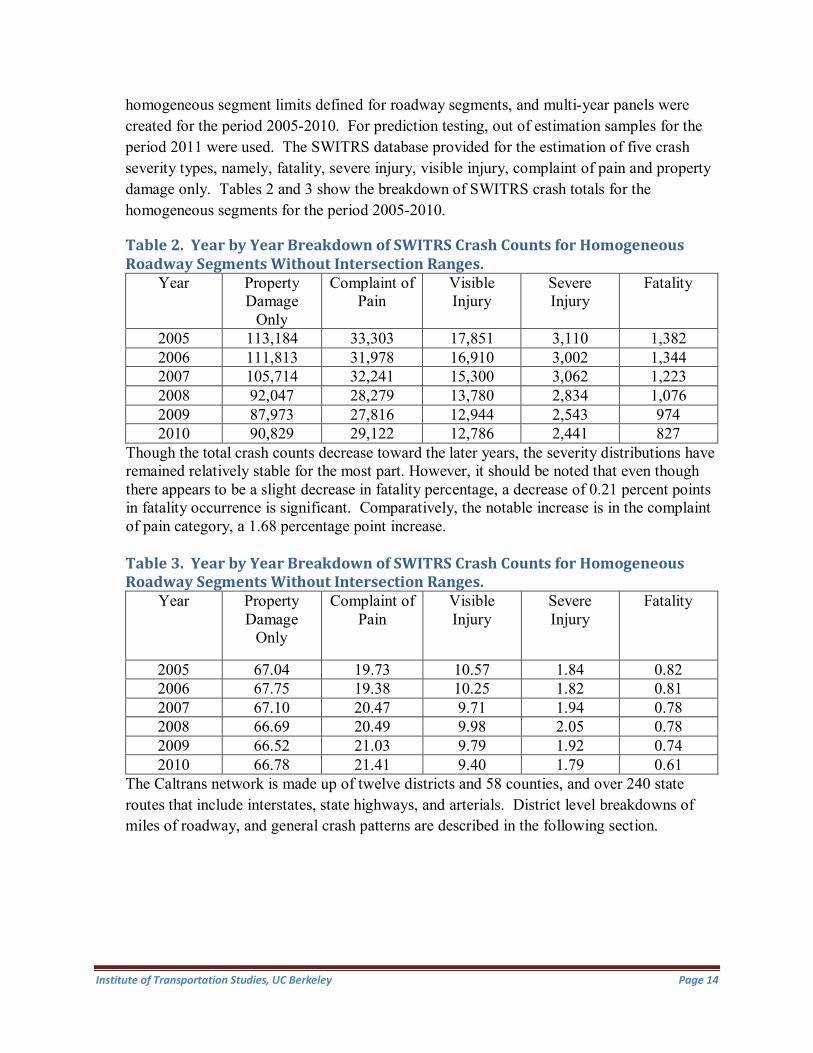
homogeneous segment limits defined for roadway segments, and multi-year panels were created for the period 2005-2010. For prediction testing, out of estimation samples for the period 2011 were used. The SWITRS database provided for the estimation of five crash severity types, namely, fatality, severe injury, visible injury, complaint of pain and property damage only. Tables 2 and 3 show the breakdown of SWITRS crash totals for the homogeneous segments for the period 2005-2010.

Table 2. Year by Year Breakdown of SWITRS Crash Counts for Homogeneous Roadway Segments Without Intersection Ranges.

Year Property Damage

Only

Complaint of Pain

Visible Injury

Severe Injury

Fatality

2005 113,184 33,303 17,851 3,110 1,382 2006 111,813 31,978 16,910 3,002 1,344 2007 105,714 32,241 15,300 3,062 1,223 2008 92,047 28,279 13,780 2,834 1,076 2009 87,973 27,816 12,944 2,543 974 2010 90,829 29,122 12,786 2,441 827

Though the total crash counts decrease toward the later years, the severity distributions have remained relatively stable for the most part. However, it should be noted that even though there appears to be a slight decrease in fatality percentage, a decrease of 0.21 percent points in fatality occurrence is significant. Comparatively, the notable increase is in the complaint of pain category, a 1.68 percentage point increase.

Table 3. Year by Year Breakdown of SWITRS Crash Counts for Homogeneous Roadway Segments Without Intersection Ranges.

Year Property Damage

Only

Complaint of Pain

Visible Injury

Severe Injury

Fatality

2005 67.04 19.73 10.57 1.84 0.82 2006 67.75 19.38 10.25 1.82 0.81 2007 67.10 20.47 9.71 1.94 0.78 2008 66.69 20.49 9.98 2.05 0.78 2009 66.52 21.03 9.79 1.92 0.74 2010 66.78 21.41 9.40 1.79 0.61

The Caltrans network is made up of twelve districts and 58 counties, and over 240 state routes that include interstates, state highways, and arterials. District level breakdowns of miles of roadway, and general crash patterns are described in the following section.


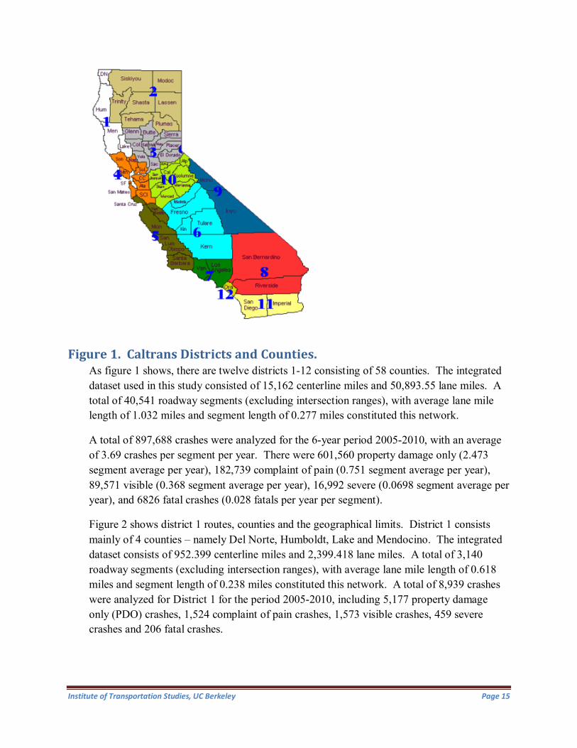
Figure 1. Caltrans Districts and Counties. As figure 1 shows, there are twelve districts 1-12 consisting of 58 counties. The integrated dataset used in this study consisted of 15,162 centerline miles and 50,893.55 lane miles. A total of 40,541 roadway segments (excluding intersection ranges), with average lane mile length of 1.032 miles and segment length of 0.277 miles constituted this network.

A total of 897,688 crashes were analyzed for the 6-year period 2005-2010, with an average of 3.69 crashes per segment per year. There were 601,560 property damage only (2.473 segment average per year), 182,739 complaint of pain (0.751 segment average per year), 89,571 visible (0.368 segment average per year), 16,992 severe (0.0698 segment average per year), and 6826 fatal crashes (0.028 fatals per year per segment).

Figure 2 shows district 1 routes, counties and the geographical limits. District 1 consists mainly of 4 counties – namely Del Norte, Humboldt, Lake and Mendocino. The integrated dataset consists of 952.399 centerline miles and 2,399.418 lane miles. A total of 3,140 roadway segments (excluding intersection ranges), with average lane mile length of 0.618 miles and segment length of 0.238 miles constituted this network. A total of 8,939 crashes were analyzed for District 1 for the period 2005-2010, including 5,177 property damage only (PDO) crashes, 1,524 complaint of pain crashes, 1,573 visible crashes, 459 severe crashes and 206 fatal crashes.


Figure 2. District 1 Routes and Counties. Figure 3 shows district 2 routes, counties and the geographical limits. District 2 consists mainly of 7 counties – namely Lassen, Modoc, Plumas, Shasta, Siskiyou, Tehama, and Trinity. The integrated dataset consists of 1,781.047 centerline miles and 4,236.959 lane miles. A total of 3,995 roadway segments (excluding intersection ranges), with average lane mile length of 0.618 miles and segment length of 0.269 miles constituted this network.

Figure 3. District 2 Routes and Counties.

A total of 10,609 crashes were analyzed for District 2 for the period 2005-2010, including 6,566 property damage only (PDO) crashes, 1,860 complaint of pain crashes, 1,587 visible crashes, 424 severe crashes and 172 fatal crashes.


Figure 4 shows District 3 routes, counties and geographical limits. District 3 consists mainly of 11 counties – namely Butte, Colusa, El Dorado, Glenn, Nevada, Placer, Sacramento, Sierra, Sutter, Yolo and Yuba. The integrated dataset consists of 1,514.463 centerline miles and 4,490.957 lane miles. A total of 3,894 roadway segments (excluding intersection ranges), with average lane mile length of 0.984 miles and segment length of 0.298 miles constituted this network.

Figure 4. District 3 Routes and Counties. A total of 60,121 crashes were analyzed for District 3 for the period 2005-2010, including 38,833 property damage only (PDO) crashes, 13,428 complaint of pain crashes, 6,128 visible crashes, 1,220 severe crashes and 512 fatal crashes.

Figure 5 shows District 4 routes, counties and geographical limits. District 4 consists of 9 counties – namely Alameda, Contra Costa, Marin, Napa, San Francisco, San Mateo, Santa Clara, Solano, and Sonoma. The integrated dataset consists of 1,395.529 centerline miles and 6,237.683 lane miles. A total of 6,062 roadway segments (excluding intersection ranges), with average lane mile length of 0.888 miles and segment length of 0.182 miles constituted this network. A total of 172,629 crashes were analyzed for District 4 for the period 2005-2010, including 117,994 property damage only (PDO) crashes, 35,531 complaint of pain crashes, 15,353 visible crashes, 2,857 severe crashes and 894 fatal crashes.


Figure 5. District 4 Routes and Counties. Figure 6 shows District 5 routes, counties and geographical limits. District 5 consists of 5 counties – namely Monterrey, San Benito, San Luis Obispo, Santa Barbara, and Santa Cruz. The integrated dataset consists of 1,153.46 centerline miles and 3,182.205 lane miles. A total of 3,233 roadway segments (excluding intersection ranges), with average lane mile length of 0.804 miles and segment length of 0.280 miles constituted this network. A total of 34,608 crashes were analyzed for District 5 for the period 2005-2010, including 23,520 property damage only (PDO) crashes, 5,942 complaint of pain crashes, 3,840 visible crashes, 972 severe crashes and 334 fatal crashes.


Figure 6. District 5 Routes and Counties. Figure 7 shows District 6 routes, counties and geographical limits. District 6 consists of 5 counties – namely Fresno, Kern, Kings, Madera and Tulare. The integrated dataset consists of 2,026.216 centerline miles and 5,726.586 lane miles. A total of 3,659 roadway segments (excluding intersection ranges), with average lane mile length of 1.169 miles and segment length of 0.376 miles constituted this network. A total of 45,174 crashes were analyzed for District 6 for the period 2005-2010, including 29,267 PDO crashes, 8,386 complaint of pain crashes, 5,651 visible crashes, 1,187 severe crashes and 683 fatal crashes.


Figure 7. District 6 Routes and Counties. Figure 8 shows District 7 routes, counties and geographical limits. District 7 consists of 2 counties – namely Los Angeles and Ventura. The integrated dataset consists of 1,134.706 centerline miles and 46,618.883 lane miles. A total of 4,378 roadway segments (excluding intersection ranges), with average lane mile length of 1.357 miles and segment length of 0.205 miles constituted this network.. A total of 268,349 crashes were analyzed for District 7 for the period 2005-2010, including 187,925 PDO crashes, 52,471 complaint of pain crashes, 23,247 visible crashes, 3,480 severe crashes and 1,226 fatal crashes.

Figure 8. District 7 Routes and Counties. Figure 9 shows District 8 routes, counties and geographical limits. District 8 consists of 2 counties – namely San Bernadino and Riverside. The integrated dataset consists of


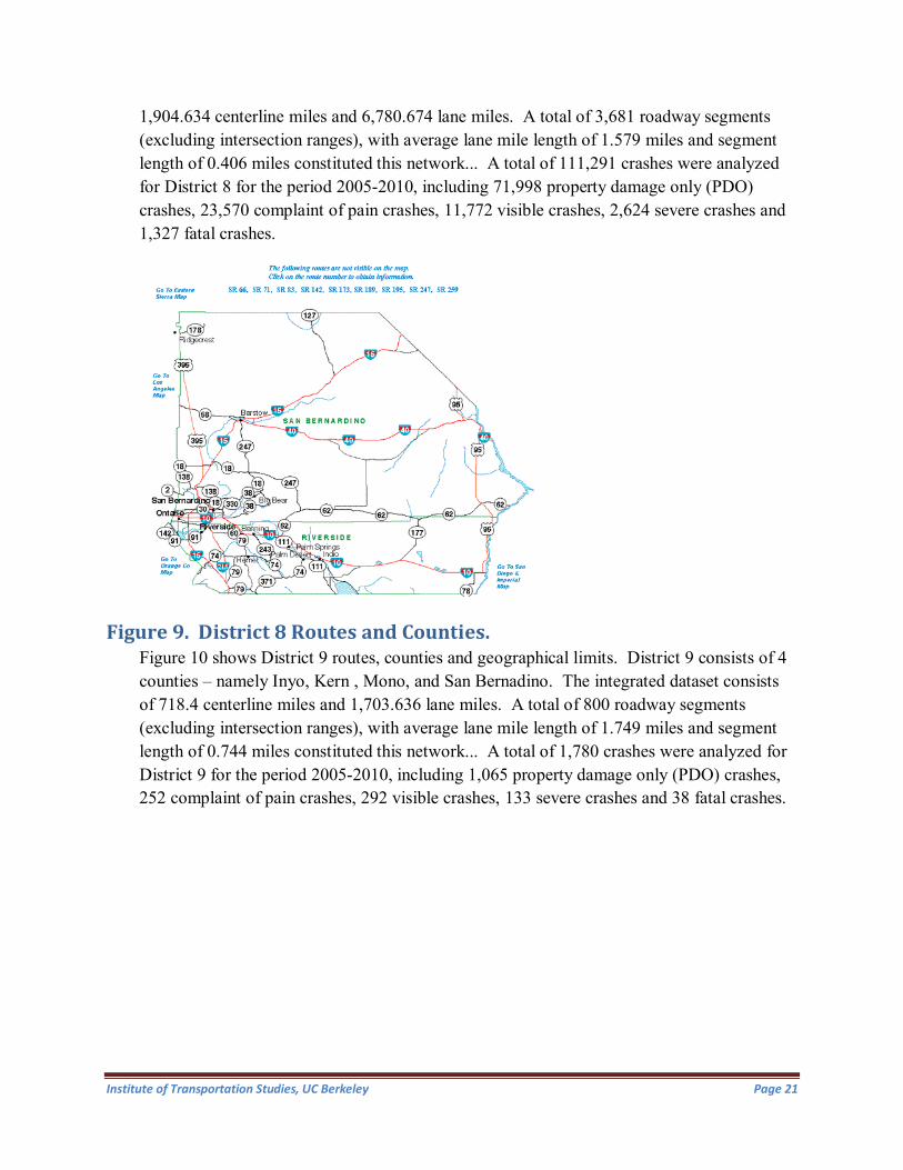
1,904.634 centerline miles and 6,780.674 lane miles. A total of 3,681 roadway segments (excluding intersection ranges), with average lane mile length of 1.579 miles and segment length of 0.406 miles constituted this network... A total of 111,291 crashes were analyzed for District 8 for the period 2005-2010, including 71,998 property damage only (PDO) crashes, 23,570 complaint of pain crashes, 11,772 visible crashes, 2,624 severe crashes and 1,327 fatal crashes.

Figure 9. District 8 Routes and Counties. Figure 10 shows District 9 routes, counties and geographical limits. District 9 consists of 4 counties – namely Inyo, Kern , Mono, and San Bernadino. The integrated dataset consists of 718.4 centerline miles and 1,703.636 lane miles. A total of 800 roadway segments (excluding intersection ranges), with average lane mile length of 1.749 miles and segment length of 0.744 miles constituted this network... A total of 1,780 crashes were analyzed for District 9 for the period 2005-2010, including 1,065 property damage only (PDO) crashes, 252 complaint of pain crashes, 292 visible crashes, 133 severe crashes and 38 fatal crashes.


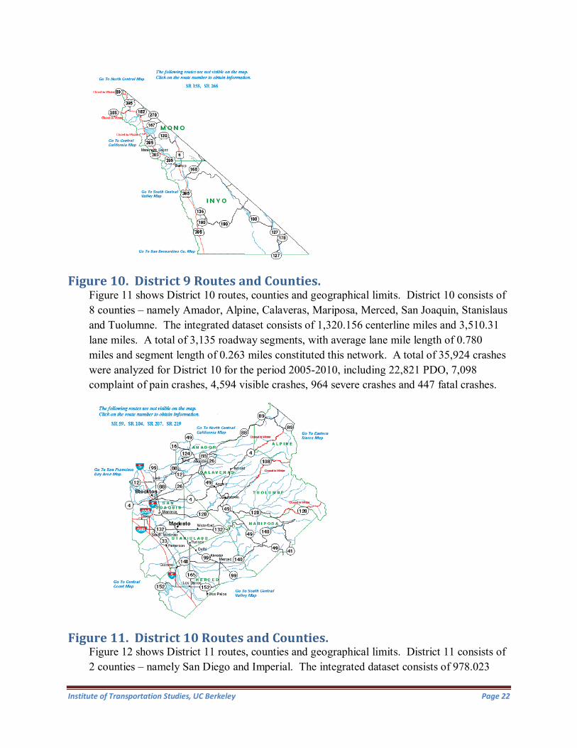
Figure 10. District 9 Routes and Counties. Figure 11 shows District 10 routes, counties and geographical limits. District 10 consists of 8 counties – namely Amador, Alpine, Calaveras, Mariposa, Merced, San Joaquin, Stanislaus and Tuolumne. The integrated dataset consists of 1,320.156 centerline miles and 3,510.31 lane miles. A total of 3,135 roadway segments, with average lane mile length of 0.780 miles and segment length of 0.263 miles constituted this network. A total of 35,924 crashes were analyzed for District 10 for the period 2005-2010, including 22,821 PDO, 7,098 complaint of pain crashes, 4,594 visible crashes, 964 severe crashes and 447 fatal crashes.

Figure 11. District 10 Routes and Counties. Figure 12 shows District 11 routes, counties and geographical limits. District 11 consists of 2 counties – namely San Diego and Imperial. The integrated dataset consists of 978.023


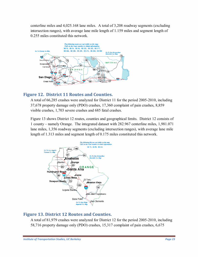
centerline miles and 4,025.168 lane miles. A total of 3,208 roadway segments (excluding intersection ranges), with average lane mile length of 1.159 miles and segment length of 0.255 miles constituted this network.

Figure 12. District 11 Routes and Counties. A total of 66,285 crashes were analyzed for District 11 for the period 2005-2010, including 37,678 property damage only (PDO) crashes, 17,360 complaint of pain crashes, 8,859 visible crashes, 1,703 severe crashes and 685 fatal crashes.

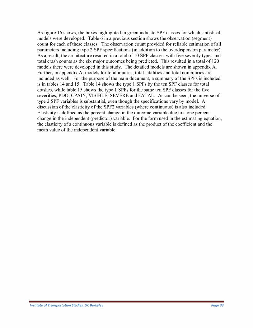
Figure 13 shows District 12 routes, counties and geographical limits. District 12 consists of 1 county – namely Orange. The integrated dataset with 282.967 centerline miles, 1,981.071 lane miles, 1,356 roadway segments (excluding intersection ranges), with average lane mile length of 1.313 miles and segment length of 0.175 miles constituted this network.

Figure 13. District 12 Routes and Counties. A total of 81,979 crashes were analyzed for District 12 for the period 2005-2010, including 58,716 property damage only (PDO) crashes, 15,317 complaint of pain crashes, 6,675


visible crashes, 969 severe crashes and 302 fatal crashes. To summarize the district level crash characteristics with respect to roadway segments, Table 4 shows the details below.

Table 4. District Level Distributions of Crash Frequencies by Severity on Roadway Segments for the period 2005-2010.

District Lane Miles

Total Segment Length (Miles)

PDO CPAIN VISIBLE SEVERE FATAL Total

1 1,941.487 747.419 5,177 1,524 1,523 459 206 8,939 2 2,715.502 1,072.741 6,566 1,860 1,587 424 172 10,609 3 3,832.659 1,160.735 38,833 13,428 6,128 1,220 512 60,121 4 5,382.614 1,100.713 117,994 35,531 15,353 2,857 894 172,629 5 2,599.617 907.532 23,520 5,942 3,840 972 334 34,608 6 4,275.709 1,375.299 29,267 8,386 5,651 1,187 683 45,174 7 5,939.087 899.359 187,925 52,471 23,247 3,480 1,226 268,349 8 5,812.746 1,493.365 71,998 23,570 11,772 2,624 1,327 111,291 9 1,399.544 595.443 1,065 252 292 133 38 1,780

10 2,445.609 823.892 22,821 7,098 4,594 964 447 35,924 11 3,717.372 817.559 37,678 17,360 8,859 1,703 685 66,285 12 1,780.678 237.02 58,716 15,317 6,675 969 302 81,979 All

Districts 601,560 182,739 89,571 16,992 6,826 897,688

Table 5. District Level Severity Distributions for the Period 2005-2010. District PDO CPAIN VISIBLE SEVERE FATAL Total

1 57.91 17.05 17.60 5.13 2.30 100 2 61.89 17.53 14.96 4.00 1.62 100 3 64.59 22.33 10.19 2.03 0.85 100 4 68.35 20.58 8.89 1.65 0.52 100 5 67.96 17.17 11.10 2.81 0.97 100 6 64.79 18.56 12.51 2.63 1.51 100 7 70.03 19.55 8.66 1.30 0.46 100 8 64.69 21.18 10.58 2.36 1.19 100 9 59.83 14.16 16.40 7.47 2.13 100 10 63.53 19.76 12.79 2.68 1.24 100 11 56.84 26.19 13.37 2.57 1.03 100 12 71.62 18.68 8.14 1.18 0.37 100 All

Districts 67.01 20.36 9.98 1.89 0.76 100

Table 5 shows the equivalent severity distributions by districts. As can be seen, the severity distributions are not homogeneous across districts. This may be indicative of collision priorities that can be strategized at the district level as well. For example, districts


1,2,6,8,9,10 and 11 have lower PDO percentages and higher severe+fatal percentages compared to the whole network. District 5 appears comparable in terms of PDO percentage, but appears to have a higher severe+fatal percentage. District 3 on the other hand has a lower PDO percentage but a comparable severe+fatal percentage compared to the whole network. District 4, 7 and 12 appear to be lower on PDO percentages and lower on the severe+fatal percentages as well compared to the whole network.

Segment Length Distributions Segment length distributions were examined by SPF class. A total of 11 SPF classes were created based on rural-urban distinctions and lane cross section leading to the following: a) two-lane rural, b) four-lane rural, c) four-plus-rural, d) multilane undivided rural, e) multilane divided, f) two-lane urban, g) four-lane urban, h) five-to-seven lane urban, i) eight or more lane urban, j) multilane undivided urban, and k) multilane divided urban. Table 6 shows the distribution of segment lengths in the above mentioned SPF classes. As seen in Table 6, 59.70% of the network has segment lengths less than or equal to 0.1 miles. The percentages vary by SPF class for lengths less than or equal to 0.1 miles. This has implications for network screening. If the distribution of segment lengths less than or equal to 0.05 miles is used, then, the average percentage for the entire network is 44.08%. Table 6. Segment Length Distributions by SPF Class (Segment Count in Parentheses).

SPF Class <=0.1 mi <=0.2 mi <=0.3 mi <=0.4 mi <=0.5 mi <=1 mi 2-lane rural

(4,202) 50.00% 60.11% 67.42% 72.68% 76.80% 86.51%

4-lane rural (9,149)

55.98% 67.46% 73.77% 78.02% 81.54% 90.45%

4-plus-rural (220)

55.45% 63.64% 72.73% 77.73% 81.36% 92.27%

Multilane undivided rural (114)

36.84% 50.00% 64.04% 75.44% 78.07% 91.23%

Multilane divided rural (33)

75.76% 81.82% 87.88% 87.88% 90.91% 93.94%

2-lane urban (5,598)

67.76% 76.99% 82.51% 86.67% 89.42% 95.61%

4-lane urban (7,182)

61.97% 74.77% 80.94% 84.68% 87.52% 94.37%

5-to-7-lane urban (4,268) 60.33% 75.75% 83.15% 87.18% 89.55% 95.15% 8-plus-urban (5,694) 48.24% 68.77% 80.80% 86.97% 90.60% 96.82%

Multilane undivided urban (845)

76.45% 84.50% 88.76% 92.07% 93.25% 97.75%

Multilane divided urban (3,236)

79.64% 88.32% 91.66% 93.79% 95.18% 98.30%

All Classes 59.70% 72.33% 79.28% 83.61% 86.64% 93.63% The high percentage of lengths under 0.1 miles is due to the fact that several geometric elements are used to determine homogeneous segments. These definitions affect the


specification of estimating models. If the lengths are altered to decrease sensitivity to geometric criteria, then, the implications for model development are significant. For example, models where a particular geometric variable is found to be significant by the universal homogeneous geometry definition, will require a modified definition if that variable is removed from the homogeneity criteria list for the purpose of decreased homogeneity sensitivity. As a result, one can have models with homogeneous geometric variables and non-homogeneous geometric variables, which can contribute to inconsistent model estimation. This is a significant estimation issue that should not be overlooked at the expense of simplified segmentation assumptions for the purpose of network screening. Network screening therefore might involve an involved iterative process where based on the model specifications, segmentations can be redefined based on the identified geometric universe of statistically significant variables. This is the preferred approach versus the alternative approach where network screening involves SPF specific windows, based on the SPF specific model variables.

Intersection Dataset for SPFs A total of 17,200 intersections were assembled using the integration of mainline roadway segment geometrics and intersection specific attributes. The following conditions were used to define intersections: a) Locate postmile of intersection as centerline postmile of mainline segmentation dataset b) Isolate mainline intersection range as consisting of +/- 0.05 mile w.r.t centerline

postmile c) Determine total crash count and SWITRS injury counts for the period 2005-2010 d) Merge mainline segment geometry from roadway segment dataset to match the +/- 0.05

mile intersection range e) Intersection range can have multiple segments f) Use minimum and maximum geometry values for continuous variables g) Use dummy value of 1 if a dummy variable is valued at 1 in at least one segment(s) in

the intersection range It should be noted here that mainline intersection crashes are being analyzed in the development of intersection SPFs since cross street crash histories were not available. The six-year period 2005-2010 was used to derive SWITRS crash counts by severity type for the 17,200 intersections. Table 7 shows the distribution of severities for this period. Table 7. Six-Year Severity Distributions for State Route Intersections. PDO CPAIN VISIBLE SEVERE FATAL TOTAL Severity Count 76,338 32,835 14,805 3,248 1,161 128,387 Severity Percentage

59.46% 25.58% 11.53% 2.53% 0.90% 100%

A balanced panel of intersections was used for the six year period, meaning every intersection has 6 years of crash history. A total of 128,387 crashes were analyzed over the


six year period (does not include cross street crashes). Intersection related mainline crashes account for roughly 13.8% of all mainline and ramp crashes, while intersection related lengths constituted less than 700 miles of the network on state route mainlines. A total of 76,338 property damage only crashes, 32,835 complaint of pain crashes, 14,805 visible injury, 3,248 severe injury crashes were analyzed and 1,161 fatal crashes were analyzed. Intersection characteristics in terms of geometry and traffic control had substantial heterogeneity. The route specific geometric heterogeneity also contributed to this effect. For example, 126 state routes had at least 30 intersections which would imply a substantial percentage of the non-freeway network (126 routes out of 213 routes used in the 17,200 intersection sample) had route specific geometric variations affecting intersection crash performance. This might also be contributing to the shift in the severity distribution toward the higher severities (3.43% for severe+fatal at intersections versus 2.65% for severe+fatal for roadway segments) due to their interactions with the multidirectional flows that occur at intersections. Table 8 shows the distribution of key intersection characteristics.

Intersection Characteristic Count Percentage Divided Mainline 5,994 34.85% Undivided Mainline 10,881 63.26% Rural 9,971 57.97% Urban 5,052 29.37% Suburban 2,178 12.66% T-intersection 9,943 57.81% Four-way intersection 5,337 31.03% Y-intersection 1,015 5.90% Five-leg intersection 146 0.85% Offset-intersection 174 1.01% No-control 587 3.41% Stop-controlled cross street 12,141 70.59% Four-way stop 81 0.47% Two-phase pretimed 253 1.47% Two-phase semiactuated 119 0.69% Two-phase fully actuated 227 1.32% Multi-phase fully actuated 1,722 10.01% Lighted intersection 8,032 46.7% Mainline mastarm 2,270 13.20% No mainline left turn lane 10,855 63.11% Painted mainline left turn lane 4,807 27.95% Mainline left turn lane with curb 1,469 8.54% No mainline right turn lane 15,332 89.14%

The characteristics shown above in Table 8 were evaluated along with segment level attributes of the mainline passing through the intersection. As mentioned before, mainline attributes such as shoulder widths, number of lanes, roadside treatments (median barrier, guardrail for example) were integrated to form a comprehensive intersection geometric


attribute dataset. Still, certain key intersection variables were missing – such as alignment data and cross street geometry. Such omitted variable effects can contribute to overdispersion in the crash models due to heterogeneity that arises from the missing geometric effects. How these overdispersion effects vary by severity is evaluated through type 2 SPFs for intersection models as discussed in a following section. As Table 8 shows, the heterogeneity in observed geometry is significant, from five-leg geometry being present at 174 intersections to absence of mainline right turn lane at 15,332 intersection sites.

Ramp Dataset Ramp information was obtained from the web using the ramp volume data on the Caltrans website. The information included 14,394 ramps containing a subset of metered ramps as well. The distribution of ramps is heterogeneous by districts, as shown in Table 9 below. Table 9. Ramp Distribution by District.

District Off-Ramp On-Ramp Directional Ramps

Total

1 146 157 20 325 2 151 178 30 359 3 505 612 51 1,169 4 1,255 1,527 252 3,037 5 359 388 1 798 6 436 542 88 1,067 7 1,364 1,738 347 3,452 8 606 642 45 1,293 9 2 7 5 14 10 133 157 24 314 11 675 808 63 1,647 12 359 474 81 919

Table 10. Ramp Crash Distribution by District.

District PDO CPAIN VISIBLE SEVERE FATAL Total 1 401 96 64 12 0 573 2 637 250 123 14 11 1,035 3 6,186 2,331 847 144 43 9,551 4 19,831 6,019 2,395 462 125 28,832 5 3,290 812 401 91 22 4,616 6 4,403 1,412 601 126 43 6,585 7 32,561 8,818 4,244 575 212 46,140 8 10,418 3,250 1,153 185 65 15,071 9 10 2 2 0 2 16

10 1,175 363 179 28 9 1,754 11 7,728 3,831 1,822 306 78 13,625 12 9,334 2,723 1,348 182 53 13,641


As tables 10 and 11 show, the distribution of severities across districts is in general consistent with what one would expect of ramp crashes – a diminished fatal+severe percentage compared to mainline crashes. District 9 appears to deviate from this norm but that is due to a low number of total crashes, which can cause even a total of 2 fatal crashes to appear as a high fatal+severe percentage of 12.5%. Table 11. Ramp Crash Distribution by Severity Percentage.

District PDO CPAIN VISIBLE SEVERE FATAL Total 1 69.98 16.75 11.17 2.09 0.00 100 2 61.55 24.15 11.88 1.35 1.06 100 3 64.77 24.41 8.87 1.51 0.45 100 4 68.78 20.88 8.31 1.60 0.43 100 5 71.27 17.59 8.69 1.97 0.48 100 6 66.86 21.44 9.13 1.91 0.65 100 7 70.16 19.00 9.14 1.24 0.46 100 8 69.13 21.56 7.65 1.23 0.43 100 9 62.50 12.50 12.50 0.00 12.50 100 10 66.99 20.70 10.21 1.60 0.51 100 11 56.14 27.83 13.24 2.22 0.57 100 12 68.43 19.96 9.88 1.33 0.39 100

A subset of this ramp system was also evaluated for crash propensities. The ramp metering subsystem contains 2,802 metered locations according to the 2013 Caltrans ramp development report (RMDP). Table 12 shows the locations by district and Table 13 shows the crash distributions for the 2,164 locations that are operational with measured ADT values and ramp type information. This information is used to generate type 1 SPFs for ramps. Table 12. District Level Distribution of Ramp Meters and Ramp Meter Dataset Distribution by District Comparison.

2013 RMDP Data Evaluated Dataset Locations Dist. Existing Planned L H C S D Total

1 0 0 0 0 0 0 0 0 2 1 10 0 0 0 0 0 0 3 189 163 43 0 0 77 0 120 4 637 684 87 0 48 174 19 328 5 3 10 1 0 0 2 0 3 6 64 111 20 0 0 38 0 58 7 999 69 199 230 20 405 0 854 8 209 224 19 0 0 190 0 209 9 0 0 0 0 0 0 0 0

10 2 167 1 0 0 1 0 2 11 310 130 54 58 12 162 0 289** 12 345 2 106 56 0 139 0 301

** Includes 3 direct ramps


As shown in Table 12, several districts have a large number of meters planned for in the near future (3, 4, 6, 8, 10 and 11 in particular). The evaluated dataset locations (2,164 sites) are shown in the right side of Table 12 and did not include districts 1, 2 and 9. Five major ramp types are evaluated (L for loop, H for hook, C for freeway-to-freeway connector, S for slip/diagonal, D for collector-distributor, see Figure 14). The majority of the evaluated ramp types are slip/diagonal or loop. To a smaller extent the hook configuration appears prominently in the District 7, 11 and 12 systems evaluation. Collector/distributor configurations are evaluated in District 4 alone.

Figure 14. Ramp Metering System Configuration Types.


Table 13. Ramp Metering System Crash Distributions.

District PDO CPAIN VISIBLE SEVERE FATAL Total 3 145 53 14 2 1 215 4 2,565 784 275 34 12 3,670 5 17 13 1 0 0 31 6 432 124 38 9 3 606 7 452 118 55 5 3 633 8 230 73 20 3 1 327

10 8 1 0 0 0 9 11 213 111 53 8 3 388 12 2,839 791 376 38 9 4,053

For type 2 SPFs for ramps, additional information relating to number of lanes, HOV meter presence and ramp type (for example, loop, slip, etc.) is required on a consistent basis for all observations. Considering the initial set of 2,162 sites, ADT, meter, HOV and ramp type information was available for 803 locations. The significant attrition in the ramp metering dataset is due to the absence of identifying information for number of lanes on the ramp and the HOV metering aspect. Quite a few sites had zero number of lanes or blanks for the number of lanes value. There are three typical characters used for defining HOV metering (using the HOVPL designation of Caltrans) – N or NM for no HOV meter, and M for HOV meter. Quite a few sites had blanks for the HOVPL column.

Safety Performance Function Development

Roadway Segment SPFs Safety performance functions for roadway segments were developed on the basis of classifications of roadways. The Federal Highway Administration (FHWA) provides for a table that characterizes roadway functional classes with respect to a range of ADTs on the roadways. Figure 15 shows the suggested functional class definitions.


Figure 15. Typical Functional Characteristics (per FHWA).

Using the information in figure 15, the following parameters were used as the basis for defining urban and rural functional thresholds: An upper ADT bound of 35,000 was used to define rural interstate freeways. Comparatively, a lower ADT bound of 13,000 was used for urban state freeways and expressways. Finally, a lower ADT bound of 3,000 was used for urban non-freeways/non-expressways, including arterials. Using these definitions, the following SPF architecture was developed, as shown in figure 16.

Figure 16. Type 1 and Type 2 SPF Modeling Architecture.


As figure 16 shows, the boxes highlighted in green indicate SPF classes for which statistical models were developed. Table 6 in a previous section shows the observation (segment) count for each of these classes. The observation count provided for reliable estimation of all parameters including type 2 SPF specifications (in addition to the overdispersion parameter). As a result, the architecture resulted in a total of 10 SPF classes, with five severity types and total crash counts as the six major outcomes being predicted. This resulted in a total of 120 models there were developed in this study. The detailed models are shown in appendix A. Further, in appendix A, models for total injuries, total fatalities and total noninjuries are included as well. For the purpose of the main document, a summary of the SPFs is included is in tables 14 and 15. Table 14 shows the type 1 SPFs by the ten SPF classes for total crashes, while table 15 shows the type 1 SPFs for the same ten SPF classes for the five severities, PDO, CPAIN, VISIBLE, SEVERE and FATAL. As can be seen, the universe of type 2 SPF variables is substantial, even though the specifications vary by model. A discussion of the elasticity of the SPF2 variables (where continuous) is also included. Elasticity is defined as the percent change in the outcome variable due to a one percent change in the independent (predictor) variable. For the form used in the estimating equation, the elasticity of a continuous variable is defined as the product of the coefficient and the mean value of the independent variable.


Table 14. Type 1 SPFs for Roadway Segments for Total Crashes.*

SPF Class α β θ

2-lane rural -5.13 0.68 1.19 4-lane rural -4.36 0.60 1.18 4-plus-rural 1.52 0.12 3.12

Multilane undivided rural -4.49 0.60 0.98 2-lane urban -7.09 0.98 2.18 4-lane urban -5.78 0.82 1.40

5-to-7-lane urban -6.49 0.89 0.91 8-plus-urban -10.75 1.24 0.64

Multilane undivided urban -5.86 0.91 3.36 Multilane divided urban -7.11 1.01 2.62

*All coefficients significant at 95% or better 𝛼𝛼 𝑖𝑖𝑖𝑖 𝑐𝑐𝑐𝑐𝑙𝑙𝑐𝑐𝑐𝑐𝑖𝑖𝑐𝑐𝑖𝑖𝑙𝑙𝑙𝑙𝑙𝑙 𝑐𝑐𝑐𝑐𝑓𝑓 𝑐𝑐𝑐𝑐𝑙𝑙𝑖𝑖𝑙𝑙𝑐𝑐𝑙𝑙𝑙𝑙 (𝑖𝑖𝑙𝑙𝑙𝑙𝑙𝑙𝑓𝑓𝑐𝑐𝑙𝑙𝑖𝑖𝑙𝑙) 𝛽𝛽 𝑖𝑖𝑖𝑖 𝑐𝑐𝑐𝑐𝑙𝑙𝑐𝑐𝑐𝑐𝑖𝑖𝑐𝑐𝑖𝑖𝑙𝑙𝑙𝑙𝑙𝑙 𝑐𝑐𝑐𝑐𝑓𝑓 𝑙𝑙𝑙𝑙(𝐴𝐴𝐴𝐴𝐴𝐴) 𝜃𝜃 𝑖𝑖𝑖𝑖 𝑐𝑐𝑜𝑜𝑙𝑙𝑓𝑓𝑜𝑜𝑖𝑖𝑖𝑖𝑖𝑖𝑙𝑙𝑓𝑓𝑖𝑖𝑖𝑖𝑐𝑐𝑙𝑙 𝑖𝑖𝑐𝑐𝑓𝑓𝑐𝑐𝑝𝑝𝑙𝑙𝑙𝑙𝑙𝑙𝑓𝑓 Table 15. Type 1 SPFs for Roadway Segments for PDO, CPAIN, VISIBLE, SEVERE and FATAL crash types.

SPF Class PDO CPAIN VISIBLE SEVERE FATAL α β θ α β θ α β θ α β θ α β θ

2-lane rural -6.36 0.75 1.15 -7.66 0.77 1.48 -6.04 0.59 1.38 -4.95 0.31 1.39 -6.71 0.40 0.74 4-lane rural -5.55 0.66 1.20 -5.42 0.50 1.41 -4.73 0.42 0.89 -4.58 0.27 0.75 -7.14 0.47 0.41 4-plus-rural 1.08 0.12 3.56 -0.95 0.20 6.08 -5.10 0.52 1.43 -9.06 0.75 0.23 -0.37 -0.20 0.59

Multilane undivided rural** -5.80 0.70 1.29 -2.34 0.09 0.47 -9.94 1.08 2.48 -6.49 0.46 -20.17 1.98 2-lane urban -8.81 1.11 2.62 -9.39 1.04 2.72 -5.66 0.56 1.43 -7.24 0.61 2.17 -7.68 0.56 1.29 4-lane urban -7.60 0.94 1.43 -8.40 0.90 1.58 -8.61 0.85 0.65 -8.33 0.67 0.55 -7.70 0.53 0.69

5-to-7-lane urban -8.64 1.04 0.91 -9.17 0.98 0.79 -9.35 0.92 0.44 -8.64 0.70 0.37 -7.84 0.55 0.32 8-plus-urban -12.43 1.35 0.70 -13.09 1.30 0.52 -10.40 1.00 0.33 -10.04 0.82 0.24 -8.07 0.57 0.19

Multilane undivided urban -6.13 0.89 4.25 -11.08 1.26 4.28 -6.22 0.67 3.11 -4.76 0.35 1.12 -9.39 0.75 0.40 Multilane divided urban -7.23 0.97 3.05 -12.06 1.35 3.21 -9.87 1.03 2.27 -9.60 0.83 1.59 -7.18 0.51 0.28 All coefficients significant at 95% or better (exceptions: 4-lane rural OD) ** poisson model for severe and fatal severity types


Tables 16-20 present type 2 SPFs for rural two-lane roadway segments.

Table 16. Rural Two-lane SPF 2 – Property Damage Only Collision Counts. Variable Mean Standard

Error T-

statistic Constant -5.43 0.22 -24.43 Logarithm of ADT 0.86 0.03 29.65 DES_SP -0.03 0.002 -14.04 IMP -0.65 0.16 -4.06 VEN 0.60 0.09 6.32 INY -0.63 0.12 -5.30 RT140 0.74 0.16 4.60 RT88 0.63 0.12 5.15 RT32 0.36 0.17 2.11 RT146 2.02 0.15 13.07 YEAR06 -0.15 0.06 -2.32 YEAR07 -0.17 0.07 -2.56 YEAR08 -0.22 0.07 -3.33 YEAR09 -0.29 0.07 -4.17 YEAR10 -0.18 0.07 -2.61 Scale parameter for overdispersion

0.81 0.06 14.42

Log-likelihood at convergence

-8,920.207

Number of observations 25,218 Table 17. Rural Two-lane SPF 2 – Complaint of Pain Collision Counts.

Variable Mean Standard Error

T-statistic

Constant -5.96 0.33 -17.93

Logarithm of ADT 0.87 0.05 19.23 Logarithm of length of segment in miles

1.0

DES_SP -0.05 0.004 -13.64 SIS -0.49 0.19 -2.55 SJ 0.83 0.45 1.84 RT88 0.94 0.19 4.86 RT32 0.49 0.24 2.00 SDIEGO 0.41 0.13 3.18 Scale parameter for overdispersion

0.88 0.13 6.69

Number of observations 25,218 As noticed in tables 16 and 17, in addition to design speed, the majority of statistically significant effects are county and route dummies. Year specific dummies represent time related shifts in specific years, such as 2006, for example. For specifying year dummies, year 2005 is used as the baseline. A negative sign for year specific dummies indicates that crashes are expected to be fewer in that year compared to year 2005.


Table 18. Rural Two-lane SPF 2 – Visible Injury Collision Counts. Variable Mean Standard

Error T-

statistic Constant -4.43 0.30 -14.62 Logarithm of ADT 0.68 0.04 17.28 DES_SP -0.04 0.003 -14.54 MNO -0.39 0.21 -1.86 LA 1.18 0.25 4.80 SDIEGO 0.86 0.11 7.86 RT140 0.63 0.19 3.31 RT88 0.62 0.20 3.15 RT190 -0.82 0.17 -4.78 VEN 0.78 0.12 6.72 YEAR06 -0.15 0.07 -2.06 YEAR09 -0.14 0.07 -2.02 YEAR10 -0.32 0.08 -3.89 Scale parameter for overdispersion

0.69 0.09 7.31

Number of observations 25,218 Table 19. Rural Two-lane SPF 2 – Severe Injury Collision Counts.

Variable Mean Standard Errors

T-statistic

Constant -4.81 0.41 -11.70 Logarithm of ADT 0.54 0.06 9.64 DES_SP -0.03 0.005 -6.95 LA 1.47 0.28 5.29 LT_OS_WI -0.05 0.02 -2.95 VEN 1.41 0.13 10.49 YEAR08 0.24 0.10 2.44 YEAR09 -0.30 0.12 -2.44 Scale parameter for overdispersion

0.44 0.17 2.52


-2,571.195

Number of observations 25,218 Table 20. Rural Two-lane SPF 2 – Fatal Injury Collision Counts.


T-statistic

Constant -6.54 0.65 -10.07 Logarithm of ADT 0.39 0 .09 4.35

RT140 0.73 0.40 1.83 YEAR09 -0.46 0.20 -2.30 YEAR10 -0.69 0.23 -2.96 Scale parameter for overdispersion

0.70 0.40 1.86


-1,119.706

Number of observations 25,218 As seen in tables 18-20, in addition to design speed, left outside shoulder width is statistically significant (severe injury model), with the rest of the effects being county, route and year


dummies. This indicates on the whole that for two-lane rural roadway segments, spatial effects, time effects and design effects are at play, in addition ADT. The elasticity of ADT does not exceed unity, since the coefficient directly represents the effect of a one percent change of ADT in the outcome. The highest elasticity of ADT is seen in complaint of pain outcomes, with a value of 0.87. The elasticity of design speed is highest for complaint of pain outcomes as well, with a value of -2.546, indicating a substantial elastic effect of design in two-lane rural roadways. This indicates that speed management on two-lane rural roadways can have substantive beneficial effects on safety.

Tables 21-25 present type 2 SPFs for 4-lane rural roadways. The results are interpreted along with the tables.

Table 21. Rural Four-lane SPF 2 –PDO Collision Counts. Variable Mean Standard

Error T-

statistic Constant -4.99 0.12 -41.92 Logarithm of ADT 0.82 0.01 61.81 DES_SP -0.03 0.001 -30.05 RT_IS_WI -0.01 0.005 -2.00 MESTRUC 1.48 0.06 25.81 MEBRAIL -1.00 0.08 -13.07 SB 0.89 0.06 14.87 RT29 0.49 0.05 9.33 RT2 0.81 0.09 9.24 RT23 1.02 0.08 13.55 RT198 0.74 0.07 11.40 RT84 -0.42 0.11 -3.69 RT80 1.03 0.07 14.81 RT101 0.27 0.04 6.45 YEAR06 -0.08 0.03 -2.48 YEAR07 -0.16 0.03 -4.75 YEAR08 -0.19 0.03 -5.76 YEAR09 -0.23 0.03 -6.84 YEAR10 -0.23 0.03 -6.96 Scale parameter for overdispersion

0.94 0.02 43.42


-33,902.384

Number of observations 54,894 Table 21 shows that in addition to ADT, design speed, inside right shoulder width, and median side object dummies such as structure and rail are statistically significant. In addition, county dummies (SB), route dummies and year dummies are significant. The negative sign of the year dummies indicates that crashes in year 2005 are expected to be higher than years 2006-2010. Route dummies are mixed in sign, with negative effects indicating fewer crashes than the routes not included in the model.


Table 22. Rural Four-lane SPF 2 – Complaint of Pain Collision Counts. Variable Mean Standard

Error T-

statistic Constant -5.57 0.17 -32.14 Logarithm of ADT 0.75 0.02 35.85

DES_SP -0.04 0.002 -21.52 DN 0.72 0.12 6.01 NEV 0.89 0.10 8.77 PLA 0.80 0.13 6.23 SM 0.57 0.09 6.73 SON 0.34 0.15 2.32 SB 0.72 0.12 5.86 SLO 0.26 0.09 2.95 VEN 0.60 0.14 4.21 RT29 0.82 0.08 9.97 RT12 0.89 0.12 7.55 RT2 1.31 0.12 11.28 RT5 -0.28 0.07 -4.12 RT99 0.34 0.11 3.07 RT4 0.29 0.09 3.28 RT68 1.75 0.40 4.35 RT180 0.40 0.08 4.99 RT14 -0.53 0.21 -2.48 YEAR06 -0.08 0.04 -1.91 Scale parameter for overdispersion

1.06 0.05 20.86


-15,727.764

Number of observations 54,894 Table 22 shows the results for complain of pain type 2 SPF. As seen in the table, the main geometric effect is design speed. All county dummies appear positive which indicates a higher crash frequency than counties excluded from the model. Several route dummies are also significant, but the time effects appear limited to year 2006 which indicates a lower complaint of pain crash frequency compared to other years. The significance of numerous spatial effect dummies indicates that spatial heterogeneity appears to dominate complain of pain outcomes. The elasticity of the design speed variable is high at -2.29, which indicates a 2.29% decrease in complaint of pain outcomes for a 1% decrease in design speed. The design speed effect is strongest in complaint of pain outcomes while ADT elasticity is strongest in PDO outcomes with a value of 0.82. An elasticity of unity for ADT would signify that ADT would be a linear multiplier for crash frequency while an elasticity greater than unity would indicate a super-linear (greater than unity exponent) effect. The length variable is not reported in any of the models since it is constrained to be equal to unity. Though the ADT parameter appears close to unity, the standard error indicates that is sublinear in elasticity, i.e., significantly different from unity.


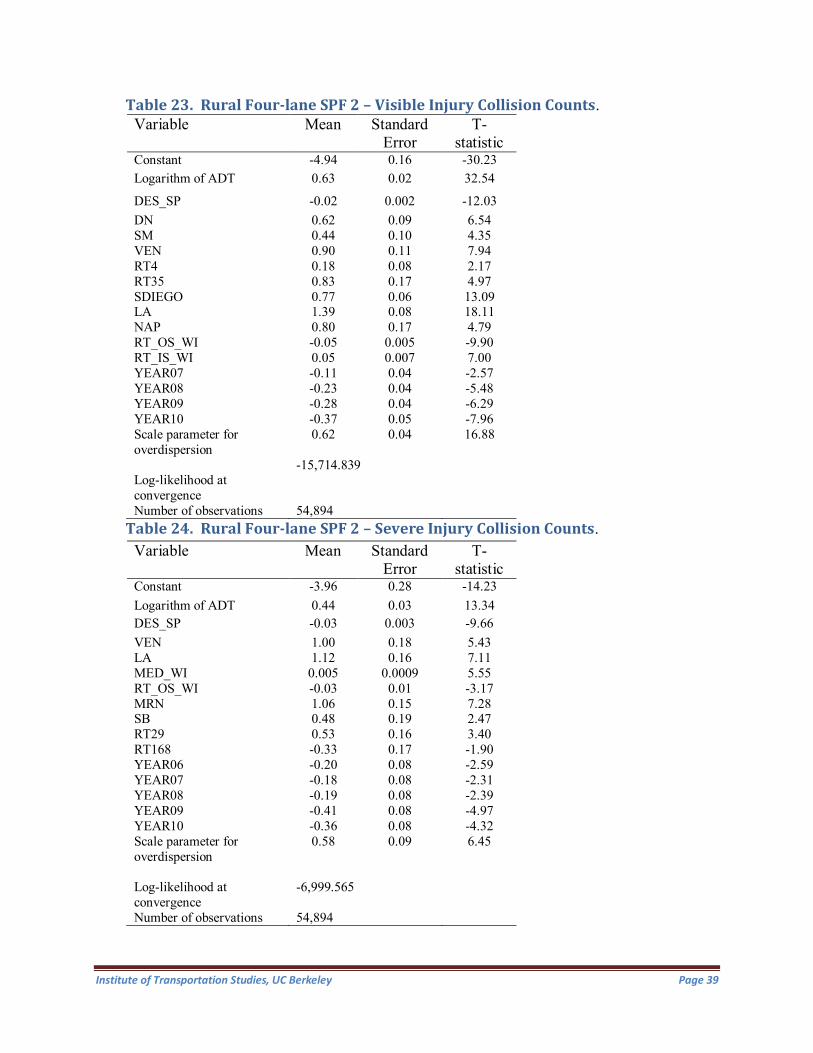
Table 23. Rural Four-lane SPF 2 – Visible Injury Collision Counts. Variable Mean Standard

Error T-

statistic Constant -4.94 0.16 -30.23 Logarithm of ADT 0.63 0.02 32.54

DES_SP -0.02 0.002 -12.03 DN 0.62 0.09 6.54 SM 0.44 0.10 4.35 VEN 0.90 0.11 7.94 RT4 0.18 0.08 2.17 RT35 0.83 0.17 4.97 SDIEGO 0.77 0.06 13.09 LA 1.39 0.08 18.11 NAP 0.80 0.17 4.79 RT_OS_WI -0.05 0.005 -9.90 RT_IS_WI 0.05 0.007 7.00 YEAR07 -0.11 0.04 -2.57 YEAR08 -0.23 0.04 -5.48 YEAR09 -0.28 0.04 -6.29 YEAR10 -0.37 0.05 -7.96 Scale parameter for overdispersion

0.62 0.04 16.88


-15,714.839

Number of observations 54,894 Table 24. Rural Four-lane SPF 2 – Severe Injury Collision Counts.


T-statistic

Constant -3.96 0.28 -14.23 Logarithm of ADT 0.44 0.03 13.34 DES_SP -0.03 0.003 -9.66 VEN 1.00 0.18 5.43 LA 1.12 0.16 7.11 MED_WI 0.005 0.0009 5.55 RT_OS_WI -0.03 0.01 -3.17 MRN 1.06 0.15 7.28 SB 0.48 0.19 2.47 RT29 0.53 0.16 3.40 RT168 -0.33 0.17 -1.90 YEAR06 -0.20 0.08 -2.59 YEAR07 -0.18 0.08 -2.31 YEAR08 -0.19 0.08 -2.39 YEAR09 -0.41 0.08 -4.97 YEAR10 -0.36 0.08 -4.32 Scale parameter for overdispersion

0.58 0.09 6.45


-6,999.565

Number of observations 54,894


Table 25. Rural Four-lane SPF 2 – Fatal Injury Collision Counts. Variable Mean Standard

Error T-

statistic Constant -7.10 0.30 -23.74 Logarithm of ADT 0.48 0.03 14.91 RT101 0.30 0.14 2.19 RT40 0.36 0.12 3.07 RT2 1.06 0.27 4.01 RT99 0.62 0.25 2.44 VEN 0.62 0.29 2.12 LAK 0.60 0.17 3.50 YEAR07 -0.18 0.09 -2.07 YEAR08 -0.26 0.09 -2.84 YEAR09 -0.27 0.09 -2.93 YEAR10 -0.49 0.10 -4.83 Scale parameter for overdispersion

N/A N/A N/A


-3,962.827

Number of observations 54,894 As seen in tables 21-25, the type 2 SPFs involve in addition to design speed, inside right shoulder width, outside right shoulder width and median width as geometric effects that are statistically significant. The maximum elasticities of inside and outside right shoulder widths are 0.05 to -0.30 indicating that the effects do not result in a greater than 1 percent change in any severity type due to a one percent change in the shoulder width. Median width similarly is inelastic with an effect of 0.14 percent change in severe injury collisions for a one percent change in median width.

Tables 26-30 show type 2 SPFs for rural four-lane-plus roadway segments.

Table 26. Rural Four-Plus-Lane SPF 2 – PDO Collision Counts. Variable Mean Standard

Error T-

statistic Constant -1.86 0.88 -2.13 Logarithm of ADT 0.34 0.08 4.23 RTLANES 0.30 0.04 7.51 LMEDHOV 1.91 0.34 5.59 MENOBARR -1.03 0.12 -8.63 SHA -0.99 0.20 -5.06 Scale parameter for overdispersion

1.49 0.12 12.56


-1,596.870



Table 27. Rural Four-Plus-Lane SPF 2 – Complaint of Pain Collision Counts. Variable Mean Standard

Error T-statistic

Constant -0.67 0.73 -1.93 Logarithm of ADT 0.10 0.07 1.39 LT_TR_WI 0.03 0.005 6.82 MENOBARR -1.90 0.15 -12.43 SHA -1.27 0.30 -4.29 YEAR05 0.25 0.16 1.77 Scale parameter for overdispersion

1.60 0.23 6.97


-821.529


Table 28. Rural Four-Plus-lane SPF 2 – Visible Injury Collision Counts. Variable Mean Standard

Error T-

statistic Constant -5.12 0.80 -6.42 Logarithm of ADT 0.46 0.08 5.89 LT_TR_WI 0.02 0.005 4.88 LMEDHOV 2.36 0.28 8.32 MENOBARR -0.65 0.15 -4.30 Scale parameter for overdispersion

0.47 0.14 3.28


-628.742


Table 29. Rural Four-Plus-Lane SPF 2 – Severe Injury Collision Counts.


T-statistic

Constant -6.01 1.44 -4.18 Logarithm of ADT 0.46 0.14 3.33 LMEDHOV 2.67 0.42 6.35 MENOBARR -0.50 0.29 -1.70 Scale parameter for overdispersion

N/A N/A N/A


-224.634



Table 30. Rural Four-Plus-Lane SPF 2 – Fatal Injury Collision Counts.


T-statistic

Constant -1.06 1.52 -1.70 Logarithm of ADT -0.08 0.16 -1.49 RT10 2.08 0.53 3.96 YEAR06 -0.69 0.42 -1.83 YEAR07 -1.02 0.49 -2.11 YEAR09 -1.03 0.49 -2.12 YEAR10 -1.95 0.73 -2.66 Scale parameter for overdispersion

N/A N/A N/A


-148.407

Number of observations 1,320 As seen in tables 26-30, the geometric effects range from continuous effects such as right travel lanes to left travel width to dummy effects such as left median side HOV lane presence and non-barriered median. The elasticity of ADT is greatest on visible and severe injury outcomes with a value of 0.46 – yet, this value is substantially lower than typical ADT elasticities. The elasticity of left travel width is greatest for complain of pain outcomes, with a value of 1.03, which indicates this effect is elastic. This suggests that a 1% percent change in left traveled width will result in a 1.03 percent increase in complaint of pain collisions on four-plus-lane rural roadways. The right travel lanes variable is near elastic with respect to PDO collisions with a value of 0.89.

Tables 31-35 show type 2 SPFs for multilane undivided rural roadway segments.

Table 31. Rural Multilane Undivided SPF 2 –PDO Collision Counts.


T-statistic

Constant -4.63 1.12 -4.12 Logarithm of ADT 0.77 0.17 4.39 DES_SP -0.03 0.01 -2.07 Scale parameter for overdispersion

1.22 0.31 3.95


-329.793

Number of observations 690 Table 31 above shows the type 2 SPF for PDO collisions on multilane undivided rural roadway segments. While ADT has an elasticity of 0.77, the elasticity of design speed is -1.64 indicating an elastic effect of design speed on PDO collisions. This indicates as found in some earlier cases, that speed management is crucial for safety on rural multilane undivided roadways. More insight on severe outcomes is discussed in the following pages.


Table 32. Rural Multilane Undivided SPF 2 –Complaint of Pain Collision Counts.


T-statistic

Constant -0.68 2.14 -0.32 Logarithm of ADT 0.19 0.26 0.74 DES_SP -0.04 0.02 -2.08 YEAR06 -0.83 0.53 -1.55 Scale parameter for overdispersion

0.19 0.51 0.38


-154.254

Number of observations 690

Table 33. Rural Multilane Undivided SPF 2 –Visible Injury Collision Counts.


T-statistic

Constant -16.14 4.01 -4.02 Logarithm of ADT 1.86 0.51 3.64 RT32 2.37 0.68 3.48 Scale parameter for overdispersion

2.03 1.22 1.87


-140.789

Number of observations 690

Table 34. Rural Multilane Undivided SPF 2 –Severe Injury Collision Counts.


T-statistic

Constant -6.18 4.68 -1.32 Logarithm of ADT 0.40 0.61 0.65 RT89 1.05 0.06 1.99 Scale parameter for overdispersion

N/A N/A N/A


-54.896

Number of observations 690 As the above tables show, design speed is the one geometric effect that is statistically significant, with an elasticity of -2.18. This is a substantial effect on complaint of pain outcomes, a pattern that appears to be repeated in several rural roadway segment categories. It is clear from the analysis of rural segments that complain of pain categories seem to be influenced by speed related effects significantly.


Table 35. Rural Multilane Undivided SPF 2 –Fatal Collision Counts.


T-statistic

Constant -21.18 13.95 -1.52 Logarithm of ADT 1.98 1.76 1.12 RT36 1.60 1.42 1.13 YEAR09 1.62 1.42 1.14 Scale parameter for overdispersion

N/A N/A N/A


-12.107

Number of observations 690 It is also observed that ADT is very elastic in its effect on fatal collisions and visible collisions. This might be suggestive of substantive interactions between truck traffic and other vehicles; suggestive of interactions resulting to head on collision types since the roadway segments are undivided.

Tables 36-40 show the results of type 2 SPFs for two-lane urban roadway segments.

Table 36. Urban Two-lane SPF 2 –PDO Collision Counts.


T-statistic

Constant -5.61 0.20 -27.66 Logarithm of ADT 0.10 0.02 50.47 DES_SP -0.03 0.001 -28.56 MEPAVE -0.56 0.10 -5.48 RT111 -0.56 0.12 -4.65 RT138 0.51 0.09 5.77 RT184 1.23 0.13 9.23 RT129 0.84 0.11 7.82 STA 0.71 0.06 12.45 SLO -0.46 0.06 -7.08 UNDIVIDE -0.45 0.04 -10.06 YEAR07 -0.12 0.03 -3.60 YEAR08 -0.23 0.04 -6.30 YEAR09 -0.30 0.04 -8.41 YEAR10 -0.33 0.04 -8.39 Scale parameter for overdispersion

2.14 0.044 48.74


-25,177.736

Number of observations 33,564 Table 36 above shows results for two-lane urban SPFs for PDO collisions. As noticed in the table, the significant geometric effect is design speed, in addition to paved median which is a dummy effect. The elasticity of the design speed variable is -1.59 which indicates an elastic effect. Spatial effects due to route and county dummies are also significant. In addition, the


undivided dummy shows a negative effect indicating that PDO collisions are expected to be lower than divided segments. All significant year dummies show a negative sign indicating that PDO crash frequencies are expected to be lower than years 2005 and 2006.

Table 37. Urban Two-lane SPF 2 – Complaint of Pain Collision Counts.


T-statistic

Constant -5.93 0.29 -20.23 Logarithm of ADT 0.93 0.03 31.62 DES_SP -0.03 0.002 -16.98 MEPAVE -0.58 0.14 -4.05 RT76 0.39 0.11 3.65 RT111 -0.68 0.20 -3.40 RT138 0.51 0.12 4.11 RT129 0.43 0.15 2.88 STA 0.80 0.08 10.44 SLO -1.15 0.16 -7.31 UNDIVIDE -0.65 0.06 -10.04 RT_OS_WI -0.01 0.006 -2.26 YEAR06 -0.17 0.06 -2.82 YEAR07 -0.19 0.06 -3.25 YEAR08 -0.27 0.06 -4.35 YEAR09 -0.27 0.06 -4.40 YEAR10 -0.37 0.06 -5.70 Scale parameter for overdispersion

2.02 0.08 25.40


-13,004.452

Number of observations 33,564 Table 38. Urban Two-lane SPF 2 –Visible Injury Collision Counts.


T-statistic

Constant -3.19 0.28 -11.41 Logarithm of ADT 0.54 0.03 20.14 DES_SP -0.02 0.002 -11.07 RT76 0.72 0.09 7.67 RT184 0.91 0.24 3.78 SLO -0.90 0.16 -5.56 UNDIVIDE -0.58 0.07 -8.36 RT_OS_WI -0.04 0.006 -7.43 YEAR08 -0.20 0.05 -3.63 YEAR09 -0.33 0.06 -5.78 YEAR10 -0.27 0.06 -4.80 Scale parameter for overdispersion

1.02 0.06 16.17


-10,097.473



Table 39. Urban Two-lane SPF 2 –Severe Injury Collision Counts.


T-statistic

Constant -4.61 0.522 -8.87 Logarithm of ADT 0.55 0.05 10.60 DES_SP -0.03 0.004 -6.94 RT76 1.11 0.14 7.80 RT129 0.66 0.24 2.79 STA 0.44 0.19 2.35 UNDIVIDE -0.53 0.12 -4.45 RT_OS_WI -0.04 0.01 -3.51 YEAR09 -0.17 0.09 -1.82 Scale parameter for overdispersion

1.61 0.21 7.68


-4,180.217


Table 40. Urban Two-lane SPF 2 –Fatal Injury Collision Counts.


T-statistic

Constant -6.87 0.66 -10.33 Logarithm of ADT 0.48 0.07 6.52 RT76 1.40 0.19 7.36 RT138 0.81 0.23 3.50 YEAR08 -0.37 0.14 -2.64 YEAR09 -0.27 0.14 -1.91 YEAR10 -0.46 0.15 -3.06 Scale parameter for overdispersion

1.09 0.35 3.08


-2,074.524

Number of observations 33,564 As seen in tables 37-40, with increasing severity of outcome, the variable outside right shoulder width appears to have a statistically significant role with a negative sign. Yet, this effect is not elastic, with a maximum of -0.22, while design speed continues to be elastic, with a value of -1.63 for severe injury collisions. In addition, the route dummies continue to have a statistically significant role spatially, with time dummies adding a temporal component, especially for years 2008-2010. What is important also to note is the significance of the overdispersion parameter for fatal injury collisions. The overdispersion parameter is 1.09, which indicates that the quadratic component involving the mean is substantial indicating heterogeneity due to unobserved effects in the urban environment. ADT has an elasticity of 0.93 for complaint of pain collisions as the maximum. This near elastic effect is suggestive of complaint of pain effects being an outcome from congestion related collisions such as rear ends or sideswipes.


Tables 41-45 shows the results for urban four-lane roadway segments.

Table 41. Urban Four-lane SPF 2 –PDO Collision Counts.


T-statistic

Constant -7.77 0.13 -60.16 Logarithm of ADT 1.10 0.01 96.90 DES_SP -0.02 0.0009 -20.00 RT15 -0.59 0.10 -5.69 RT210 -1.11 0.09 -11.90 RT2 -1.74 0.08 -21.26 RT135 1.88 0.10 18.27 RT13 1.02 0.08 12.30 RT99 -0.21 0.03 -7.47 RT101 -0.28 0.02 -11.10 LA 0.40 0.03 12.43 SON 0.33 0.03 9.78 ALA -0.45 0.04 -11.62 YUB -0.87 0.08 -10.70 MEBEAM 0.62 0.07 9.23 MESTRUC -0.44 0.04 -10.94

Table 41 shows that several geometric effects on the median side appear to be statistically significant in their impact on PDO collisions on urban four-lane roadway segments. Paved median, median guard rail beam presence, median structure presence, median ditch, as well as median stripes as dummies are significant, while median width as a continuous variable is also significant. This signifies the importance of median roadside treatment in four lane urban contexts. The effects are to decrease the crash frequencies of PDOs, with median width being -0.12 in elasticity. Design speed is significant and elastic with a value of -1.23. In addition, route, county and year dummies are significant.

MEDIT -1.17 0.38 -3.09 MESGR -0.68 0.06 -10.74 MEPAVE -0.37 0.03 -14.46 MEST -0.26 0.03 -8.37 MED_WI -0.004 0.0004 -9.14 LTLANES 0.21 0.02 8.80 YEAR06 -0.12 0.02 -4.75 YEAR07 -0.17 0.02 -7.15 YEAR08 -0.28 0.02 -11.67 YEAR09 -0.31 0.02 -13.32 YEAR10 -0.30 0.02 -13.30 Scale parameter for overdispersion

1.173

0.02

77.82


-58,921.683

Number of observations

43,104


Table 42. Urban Four-lane SPF 2 –Complaint of Pain Collision Counts.


T-statistic

Constant -8.41 0.20 -43.08 Logarithm of ADT 1.14 0.02 65.77 DES_SP -0.03 0.001 -27.25 METWTL -0.12 0.06 -1.92 RT15 -0.56 0.11 -5.30 RT210 -0.91 0.11 -8.14 RT2 -1.20 0.12 -10.00 RT135 1.82 0.13 14.12 RT13 0.49 0.12 4.18 RT99 -0.30 0.04 -8.60 RT101 -0.57 0.03 -17.31 LA 0.37 0.04 8.56 SON 0.55 0.05 11.88 ALA -0.18 0.06 -3.15 YUB -0.53 0.11 -4.98 MECONCG -0.33 0.06 -5.18 MEBEAM 0.63 0.08 7.62 MESTRUC -0.47 0.06 -7.47 MESGR -0.58 0.08 -7.59 MENPAVE -0.43 0.05 -9.47 MEPAVE -0.44 0.04 -9.89 MEST -0.38 0.05 -7.31 MED_WI -0.005 0.0006 -9.39 LTLANES 0.26 0.03 7.82 YEAR06 -0.10 0.03 -3.56 YEAR08 -0.17 0.03 -5.70 YEAR09 -0.19 0.03 -6.44 YEAR10 -0.14 0.03 -4.76 Scale parameter for overdispersion

1.19 0.02 48.54


-34,217.784

Number of observations 43,104 Similar to PDO collisions, median effects are significant in complaint of pain collisions as well, with several median dummies being negatively signed. Median width is not elastic with a value of -0.15, while left travel lanes is inelastic with a value of 0.47. Design speed is elastic with a value of -1.83 indicating that speed management is an issue for urban four lane roadways as well. The significance of route, county and yearly dummies continues to underscore the importance of spatial and temporal effects in terms of their heterogeneity. The temporal effects seem to indicate as previously seen in other type 2 SPFs that year 2005 frequencies are expected to be higher than subsequent years, 2006-2010. What is also noticeable is the significant value of the overdispersion parameter which indicates substantial residual heterogeneity even after accounting for a variety of geometric, spatial and temporal effects in the model. The ADT variable is elastic, which indicates congestion effects playing a substantial role.


Table 43. Urban Four-lane SPF 2 –Visible Injury Collision Counts.


T-statistic

Constant -7.84 0.20 -39.44 Logarithm of ADT 0.88 0.02 48.82 DES_SP -0.02 0.002 -10.53 RT2 -1.45 0.15 -9.69 RT99 -0.13 0.04 -3.66 RT101 -0.17 0.03 -5.32 LA 0.38 0.05 8.18 YUB -0.89 0.14 -6.16 MEBEAM 0.64 0.08 8.12 MESTRUC -0.19 0.07 -2.80 MESGR -0.21 0.08 -2.63 MENPAVE -0.16 0.04 -3.81 MEPAVE -0.18 0.04 -4.76 MED_WI -0.003 0.0006 -4.70 LTLANES 0.27 0.04 7.58 YEAR06 -0.07 0.03 -2.03 YEAR07 -0.25 0.04 -6.90 YEAR08 -0.33 0.04 -8.98 YEAR09 -0.36 0.04 -9.67 YEAR10 -0.42 0.04 -11.52 Scale parameter for overdispersion

0.58 0.02 28.06


-23,547.975

Number of observations 43,104 Table 44. Urban Four-lane SPF 2 –Severe Injury Collision Counts.


T-statistic

Constant -7.65 0.36 -21.28 Logarithm of ADT 0.72 0.03 20.61 DES_SP -0.02 0.003 -7.05 SCR 0.54 0.11 4.94 HUM 0.52 0.16 3.17 YEAR05 0.11 0.06 1.96 YEAR09 -0.17 0.06 -2.78 YEAR10 -0.16 0.06 -2.66 Scale parameter for overdispersion

0.55 0.07 7.71


-8,401.243



Table 45. Urban Four-lane SPF 2 –Fatal Injury Collision Counts.


T-statistic

Constant -7.51 0.47 -16.13 Logarithm of ADT 0.54 0.04 12.07 MENPAVE -0.14 0.07 -1.90 MEPAVE -0.27 0.10 -2.70 YEAR08 -0.32 0.09 -3.60 YEAR09 -0.38 0.09 -4.30 YEAR10 -0.46 0.09 -4.89 Scale parameter for overdispersion

0.63 0.14 4.64


-4,522.402

Number of observations 43,104 As seen in tables 43-45, median effects continue to affect fatal injury collision propensities with paved and non-paved medians having a negative effect, while median width is inelastic with respect to visible injury collisions.

Tables 46-50 show results for type 2 SPFs for urban 5-6-7 lane roadway segments.

Table 46. Urban Five-Six-Seven-lane SPF 2 –PDO Collision Counts.


T-statistic

Constant -8.04 0.11 -72.39 Logarithm of ADT 1.02 0.01 102.04 METWTL -0.53 0.08 -6.27 RT261 -1.50 0.19 -7.73 RT15 -0.22 0.03 -7.19 RT92 0.53 0.07 7.80 RT29 0.98 0.09 10.86 LA 0.17 0.02 8.64 MESTRUC -0.10 0.02 -4.45 FRE 0.35 0.04 8.48 MED_WI -0.007 0.0003 -27.59 YEAR07 -0.07 0.02 -3.74 YEAR08 -0.22 0.02 -10.69 YEAR09 -0.28 0.02 -13.63 YEAR10 -0.26 0.02 -12.31 Scale parameter for overdispersion

0.82 0.01 69.24


-49,388.383



Table 47. Urban Five-Six-Seven-lane SPF 2 –Complaint of Pain Collision Counts.


T-statistic

Constant -7.86 0.29 -20.23 Logarithm of ADT 1.10 0.02 70.94 DES_SP -0.03 0.001 -24.26 METWTL 0.48 0.09 5.55 RT261 -1.37 0.32 -4.32 RT15 -0.21 0.04 -5.41 RT29 1.28 0.10 12.52 SOL -0.35 0.08 -4.58 SF -0.15 0.07 -2.30 MECONCG -0.12 0.05 -2.64 MEST -0.47 0.13 -3.56 MED_WI -0.01 0.0004 -20.07 YEAR06 -0.06 0.03 -2.24 YEAR07 -0.07 0.03 -2.52 YEAR08 -0.21 0.03 -6.70 YEAR09 -0.22 0.03 -7.41 YEAR10 -0.20 0.03 -6.76 Scale parameter for overdispersion

0.69 0.02 45.34


-30,557.415

Number of observations 25,590 Table 48. Urban Five-Six-Seven-lane SPF 2 –Visible Injury Collision Counts.


T-statistic

Constant -7.62 0.22 -35.39 Logarithm of ADT 0.92 0.02 45.71 DES_SP -0.02 0.002 -9.41 FRE 0.26 0.06 4.72 LA 0.21 0.03 7.30 SOL -0.25 0.09 -2.81 MENPAVE -0.07 0.03 -2.16 MEPAVE -0.14 0.04 -3.80 MEST -0.49 0.14 -3.49 MED_WI -0.01 0.001 -9.53 YEAR06 -0.08 0.03 -2.31 YEAR07 -0.18 0.03 -5.51 YEAR08 -0.25 0.03 -7.29 YEAR09 -0.34 0.03 -9.75 YEAR10 -0.33 0.03 -9.69 Scale parameter for overdispersion

0.38 0.02 25.12


-20,783.558



Table 49. Urban Five-Six-Seven-lane SPF 2 –Severe Injury Collision Counts.


T-statistic

Constant -7.76 0.46 -16.92 Logarithm of ADT 0.72 0.04 18.55 DES_SP -0.01 0.004 -2.37 RT_OS_WI -0.03 0.01 -4.76 FRE 0.44 0.09 5.08 YEAR08 -0.14 0.06 -2.57 YEAR09 -0.18 0.06 -3.18 YEAR10 -0.19 0.06 -3.33 Scale parameter for overdispersion

0.34 0.05 6.42


-7,325.192

Number of observations 25,590 Table 50. Urban Five-Six-Seven-lane SPF 2 –Fatal Injury Collision Counts.


T-statistic

Constant -7.83 0.69 -11.43 Logarithm of ADT 0.55 0.06 9.35 RT99 0.18 0.01 2.09 RT4 0.47 0.23 2.09 YEAR08 -0.17 0.08 -2.07 YEAR09 -0.19 0.08 -2.24 YEAR10 -0.37 0.09 -4.05 Scale parameter for overdispersion

N/A N/A N/A


-3,733.609

Number of observations 25,590 As tables 46-50 show, the median effects are the significant geometric effects in addition to design speed. Median effects are generally dummy in nature, including variables such as median turnouts, median striping, paved medians, medians with concrete barriers and glare screens as well as median width. However, median width is not elastic. Right outside shoulder width is significant for severe injury collisions, although it is not elastic. Design speed is the one geometric effect that is elastic, with respect to complaint of pain and visible injury collisions. The elasticity is as high as -2.02. Spatial dummies are not as pronounced in the urban 5-6-7 lane models as noticed in other type 2 SPFs indicating a greater level of design consistency and diminished spatial heterogeneity due to route or county effects. ADT is elastic for PDO and complaint of pain collision types. This emphasizes congestion effects and the need for active traffic management strategies to mitigate lower severity outcomes. Higher severity outcomes appear to be influenced primarily by median effects or time dummies. Tables 51-55 show the results of type 2 SPFs for urban eight-plus lane roadway segments.


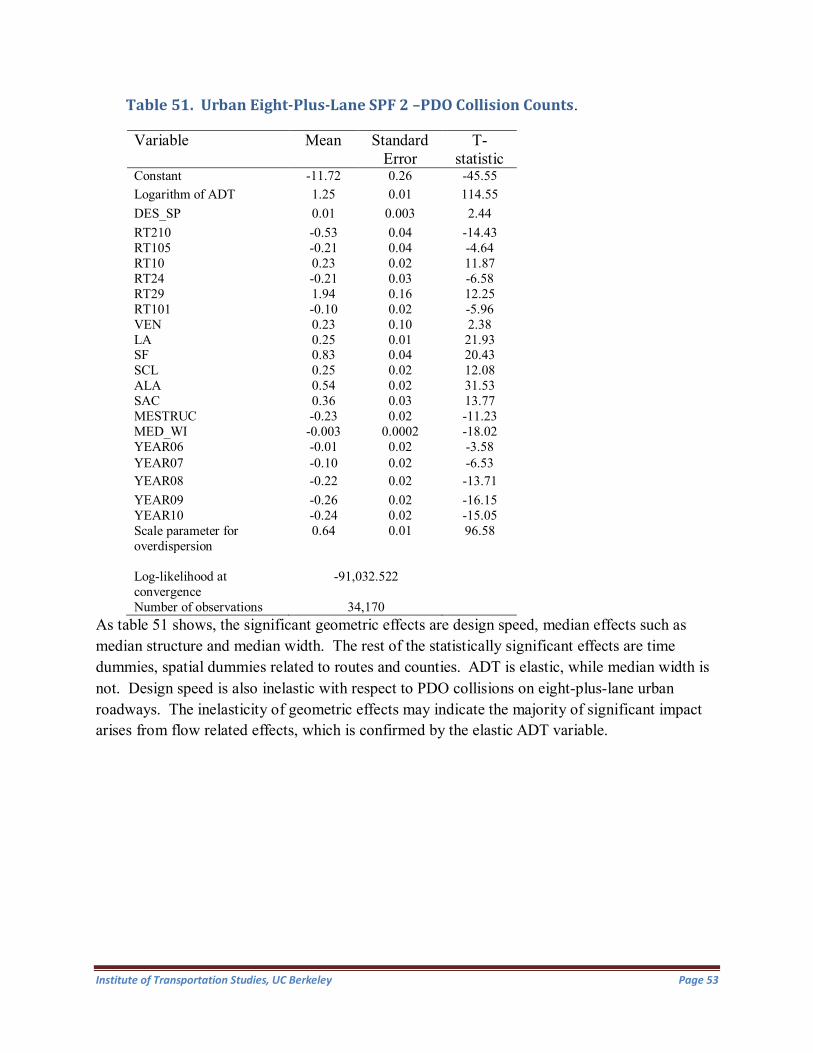
Table 51. Urban Eight-Plus-Lane SPF 2 –PDO Collision Counts.


T-statistic

Constant -11.72 0.26 -45.55 Logarithm of ADT 1.25 0.01 114.55 DES_SP 0.01 0.003 2.44 RT210 -0.53 0.04 -14.43 RT105 -0.21 0.04 -4.64 RT10 0.23 0.02 11.87 RT24 -0.21 0.03 -6.58 RT29 1.94 0.16 12.25 RT101 -0.10 0.02 -5.96 VEN 0.23 0.10 2.38 LA 0.25 0.01 21.93 SF 0.83 0.04 20.43 SCL 0.25 0.02 12.08 ALA 0.54 0.02 31.53 SAC 0.36 0.03 13.77 MESTRUC -0.23 0.02 -11.23 MED_WI -0.003 0.0002 -18.02 YEAR06 -0.01 0.02 -3.58 YEAR07 -0.10 0.02 -6.53 YEAR08 -0.22 0.02 -13.71 YEAR09 -0.26 0.02 -16.15 YEAR10 -0.24 0.02 -15.05 Scale parameter for overdispersion

0.64 0.01 96.58


-91,032.522

Number of observations 34,170 As table 51 shows, the significant geometric effects are design speed, median effects such as median structure and median width. The rest of the statistically significant effects are time dummies, spatial dummies related to routes and counties. ADT is elastic, while median width is not. Design speed is also inelastic with respect to PDO collisions on eight-plus-lane urban roadways. The inelasticity of geometric effects may indicate the majority of significant impact arises from flow related effects, which is confirmed by the elastic ADT variable.


Table 52. Urban Eight-Plus-lane SPF 2 –Complaint of Pain Collision Counts.


T-statistic

Constant -12.04 0.19 -63.61 Logarithm of ADT 1.23 0.02 78.81 RT210 -0.40 0.04 -10.43 RT24 -0.34 0.06 -6.00 RT29 2.14 0.21 10.27 LA 0.07 0.01 5.26 SF 0.61 0.06 9.59 ALA 0.29 0.02 12.87 SAC 0.43 0.03 14.78 MESTRUC -0.14 0.03 -4.55 MED_WI -0.004 0.0003 -13.51 YEAR06 -0.07 0.02 -3.66 YEAR07 -0.09 0.02 -4.43 YEAR08 -0.18 0.02 -9.52 YEAR09 -0.19 0.02 -9.76 YEAR10 -0.14 0.02 -7.40 Scale parameter for overdispersion

0.49 0.01 62.42


-58,741.044

Number of observations 34,170 Table 53. Urban Eight-Plus-lane SPF 2 –Visible Injury Collision Counts.


T-statistic

Constant -9.46 0.23 -41.22 Logarithm of ADT 0.97 0.02 49.84 RT24 -0.28 0.06 -4.26 RT29 1.19 0.31 3.88 RT_TR_WI -0.004 0.001 -5.87 SJ 0.30 0.09 3.43 MRN -0.45 0.07 -6.78 MED_WI -0.003 0.0003 -10.84 SM -0.38 0.04 -10.76 RT1 0.40 0.15 - 2.62 RT680 -0.41 0.05 -8.05 RT22 0.59 0.15 4.08 YEAR06 -0.09 0.02 -4.10 YEAR07 -0.18 0.02 -8.50 YEAR08 -0.26 0.02 -11.51 YEAR09 -0.32 0.02 -14.09 YEAR10 -0.29 0.02 -13.20 Scale parameter for overdispersion

0.29 0.01 33.42


-39,925.551



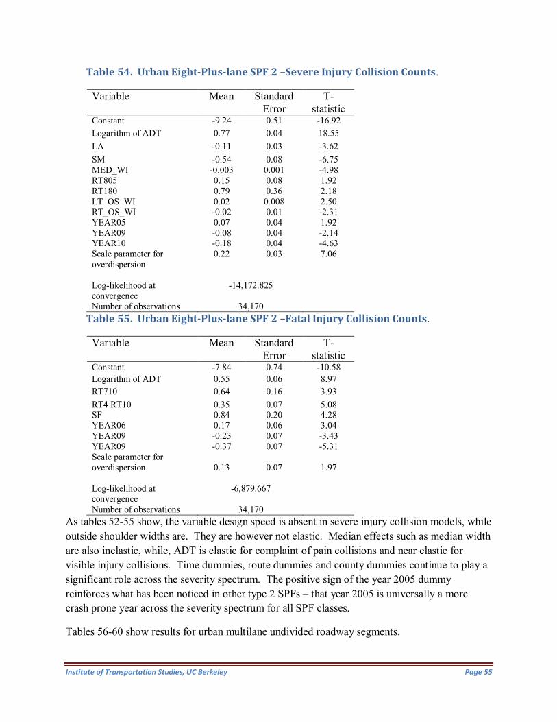
Table 54. Urban Eight-Plus-lane SPF 2 –Severe Injury Collision Counts.


T-statistic

Constant -9.24 0.51 -16.92 Logarithm of ADT 0.77 0.04 18.55 LA -0.11 0.03 -3.62 SM -0.54 0.08 -6.75 MED_WI -0.003 0.001 -4.98 RT805 0.15 0.08 1.92 RT180 0.79 0.36 2.18 LT_OS_WI 0.02 0.008 2.50 RT_OS_WI -0.02 0.01 -2.31 YEAR05 0.07 0.04 1.92 YEAR09 -0.08 0.04 -2.14 YEAR10 -0.18 0.04 -4.63 Scale parameter for overdispersion

0.22 0.03 7.06


-14,172.825

Number of observations 34,170 Table 55. Urban Eight-Plus-lane SPF 2 –Fatal Injury Collision Counts.


T-statistic

Constant -7.84 0.74 -10.58 Logarithm of ADT 0.55 0.06 8.97 RT710 0.64 0.16 3.93 RT4 RT10 0.35 0.07 5.08 SF 0.84 0.20 4.28 YEAR06 0.17 0.06 3.04 YEAR09 -0.23 0.07 -3.43 YEAR09 -0.37 0.07 -5.31 Scale parameter for overdispersion

0.13

0.07

1.97


-6,879.667

Number of observations 34,170 As tables 52-55 show, the variable design speed is absent in severe injury collision models, while outside shoulder widths are. They are however not elastic. Median effects such as median width are also inelastic, while, ADT is elastic for complaint of pain collisions and near elastic for visible injury collisions. Time dummies, route dummies and county dummies continue to play a significant role across the severity spectrum. The positive sign of the year 2005 dummy reinforces what has been noticed in other type 2 SPFs – that year 2005 is universally a more crash prone year across the severity spectrum for all SPF classes.

Tables 56-60 show results for urban multilane undivided roadway segments.


Table 56. Urban Multi-Lane Undivided SPF 2 –PDO Collision Counts.

Table 57. Urban Multi-Lane Undivided SPF 2 –Complaint of Pain Collision Counts.


T-statistic

Constant -8.95 0.88 -10.16 Logarithm of ADT 0.98 0.09 11.04 RTLANES 0.97 0.15 6.39 DES_SP -0.02 0.004 -5.12 RTRCL -1.37 0.18 -7.64 TUL 1.24 0.30 4.10 STA 1.24 0.39 3.21 RT108 -1.30 0.50 -2.58 YEAR10 -0.44 0.14 -3.11 Scale parameter for overdispersion

3.27

0.27

12.26


-2,382.162


5,064

As tables 56-60 show, the geometric effects that are statistically significant include right travel lanes, truck climbing lane dummy, and design speed. The right travel lanes variable is elastic with an elasticity of 1.90, while the design speed variable is also elastic with a value of -1.57 for PDO collisions. ADT is near elastic for complaint of pain collisions with a value of 0.98. Spatial dummies include both route and county effects which are however not as rich as some of the earlier type 2 SPFs. Time dummies include later year effects such as year 2008 and year


T-statistic

Constant -3.45 0.54 -6.38

Logarithm of ADT 0.65 0.05 13.96

RTLANES 0.77 0.09 8.70 DES_SP -0.03 0.003 -11.45 RTRCL -1.40 0.14 -9.96 TUL 1.35 0.20 6.68 RT138 YEAR08

-0.68 -0.24

0.30 0.09

-2.25 -2.75

YEAR10 -0.41 0.09 -4.51 Scale parameter for overdispersion

3.01

0.14

21.79


4,612.316


5,064


2010. The overdispersion parameter magnitude is significant indicating substantial residual heterogeneity due to unobserved effects.

Table 58. Urban Multi-Lane Undivided SPF 2 –Visible Injury Collision Counts.


T-statistic

Constant -4.89 0.87 -5.65 Logarithm of ADT 0.56 0.09 6.19 RTRCL -0.77 0.20 -3.84 SBT 1.35 0.44 3.03 YEAR08 -0.39 0.17 -2.30 YEAR09 -0.33 0.17 -1.97 YEAR10 -0.43 0.17 -2.53 Scale parameter for overdispersion

3.03

0.39

7.83


-1,626.679

Number of observations 5,064 Table 59. Urban Multi-Lane Undivided SPF 2 –Severe Injury Collision Counts.


T-statistic

Constant -4.40 1.40 -3.15 Logarithm of ADT 0.48 0.14 3.51

DES_SP -0.03 0.009 -3.12 TUL 1.33 0.55 2.42 YEAR10 -0.67 0.31 -2.13 Scale parameter for overdispersion

1.39 0.88 1.89


-593.393

Number of observations 5,064 Table 60. Urban Multi-Lane Undivided SPF 2 –Fatal Injury Collision Counts.


T-statistic

Constant -8.14 1.78 -4.56 Logarithm of ADT 0.59 0.19 3.14 RIV 0.76 0.29 2.65 RT62 1.47 0.45 3.30 YEAR06 -0.89 0.47 -1.91 NEV 1.07 0.50 2.16 Scale parameter for overdispersion

N/A N/A N/A


-300.531

Number of observations 5,064 Tables 61-65 show the type 2 SPFs for urban multilane divided roadway segments.


Table 61. Urban Multi-Lane Divided SPF 2 –PDO Collision Counts.

Table 62. Urban Multi-Lane Undivided SPF 2 –Complaint of Pain Counts. Variable Mean Standard

Error T-

statistic Constant -8.68 0.44 -19.62 Logarithm of ADT 1.09 0.04 25.44 LT_IS_WI 0.04 0.01 3.39 LTLANES 0.39 0.05 8.40 RT_IS_WI -0.07 0.01 -5.31 DES_SP -0.03 0.002 -13.57 METWTL -0.37 0.06 -6.61 MENPAVE -0.53 0.06 -9.15 MENOBARR 0.48 0.09 5.28 SCL -0.85 0.08 -10.44 VEN 1.02 0.19 5.23 RIV 0.21 0.08 2.75 MER -1.18 0.12 -9.84 IMP -1.02 0.10 -10.17 RT33 -1.09 0.26 -4.10 RT18 -0.45 0.15 -3.09 RT74 0.54 0.11 4.84 YEAR08 -0.145 0.05 -2.89 YEAR09 -0.11 0.05 -2.13 YEAR10 -0.13 0.05 -2.38 Overdispersion 2.15 0.07 29.62 Log-likelihood at convergence

-12,203.616



T-statistic

Constant -4.41 0.26 -17.17 Logarithm of ADT 0.84 0.03 31.49 RT_TR_WI 0.01 0.003 4.39 DES_SP -0.02 0.002 -14.45 METWTL -0.43 0.04 -10.33 MEPAVE -0.47 0.04 -11.18 MENPAVE MESTRUC

-0.56 -1.09

0.04 0.14

-2.25 -7.54

SCL -0.65 0.06 -10.04 SBD 0.61 0.06 11.06 MER -0.60 0.09 -6.59 IMP -0.92 0.07 -13.44 RT18 -0.46 0.09 -5.22 YEAR06 -0.14 0.05 -2.95 YEAR07 -0.21 0.05 -4.70 YEAR08 -0.39 0.05 -7.79 YEAR09 -0.44 0.05 -8.88 YEAR10 -0.52 0.05 -11.16 Overdispersion 2.55 0.05 48.00 Log-likelihood at convergence

-19,626.609



Table 63. Urban Multi-Lane Undivided SPF 2 –Visible Injury Collision Counts.


T-statistic

Constant -6.61 0.46 -14.35 Logarithm of ADT 0.80 0.05 16.59 LTLANES 0.40 0.06 6.75 RT_IS_WI -0.05 0.01 -4.58 DES_SP -0.03 0.003 -8.75 METWTL -0.20 0.07 -2.98 SCL -0.48 0.09 -5.13 RIV 0.39 0.09 4.56 SBD 0.57 0.09 5.99 IMP -0.69 0.12 -5.57 RT18 -0.59 0.19 -3.14 YEAR06 -0.21 0.08 -2.74 YEAR07 -0.43 0.08 -5.36 YEAR08 -0.41 0.08 -4.87 YEAR09 -0.49 0.08 -5.87 YEAR10 -0.53 0.08 -6.27 Scale parameter for overdispersion

1.71

0.11

15.20


-7,060.811

Number of observations 19,434 Table 64. Urban Multi-Lane Undivided SPF 2 –Severe Injury Collision Counts.


T-statistic

Constant -7.54 0.79 -9.51 Logarithm of ADT 0.67 0.09 7.81 LTLANES 0.33 0.10 3.19 DES_SP -0.02 0.005 -4.39 SCL -0.42 0.18 -2.38 Scale parameter for overdispersion

1.52 0.30 5.01


-2,187.033

Number of observations 19,434 As tables 61-65 show, the geometric effects that are statistically significant include left travel lanes, design speed, inside shoulder width, median type dummies and right travel width. Design speed is elastic, with a maximum of -1.62 for visible injury collisions, while left travel lanes is near elastic for visible injury collisions, with an elasticity of 0.84. Right outside shoulder width is significant in fatal injury collisions with a negative sign, but not elastic. ADT is elastic for complaint of pain collisions.


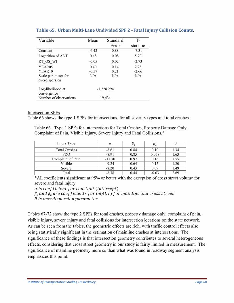
Table 65. Urban Multi-Lane Undivided SPF 2 –Fatal Injury Collision Counts.


T-statistic

Constant -6.42 0.88 -7.31 Logarithm of ADT 0.48 0.08 5.70 RT_OS_WI -0.05 0.02 -2.73 YEAR05 0.40 0.14 2.78 YEAR10 -0.57 0.21 -2.66 Scale parameter for overdispersion

N/A N/A N/A


-1,228.294


Intersection SPFs Table 66 shows the type 1 SPFs for intersections, for all severity types and total crashes.

Table 66. Type 1 SPFs for Intersections for Total Crashes, Property Damage Only, Complaint of Pain, Visible Injury, Severe Injury and Fatal Collisions.*

Injury Type α 𝛽𝛽1 𝛽𝛽2 θ

Total Crashes -8.61 0.84 0.10 1.34 PDO -8.91 0.85 0.058 1.63

Complaint of Pain -11.70 0.97 0.16 1.55 Visible -9.24 0.64 0.15 1.20 Severe -8.20 0.43 0.09 1.49 Fatal -8.38 0.44 -0.03 2.69

*All coefficients significant at 95% or better with the exception of cross street volume for severe and fatal injury 𝛼𝛼 𝑖𝑖𝑖𝑖 𝑐𝑐𝑐𝑐𝑙𝑙𝑐𝑐𝑐𝑐𝑖𝑖𝑐𝑐𝑖𝑖𝑙𝑙𝑙𝑙𝑙𝑙 𝑐𝑐𝑐𝑐𝑓𝑓 𝑐𝑐𝑐𝑐𝑙𝑙𝑖𝑖𝑙𝑙𝑐𝑐𝑙𝑙𝑙𝑙 (𝑖𝑖𝑙𝑙𝑙𝑙𝑙𝑙𝑓𝑓𝑐𝑐𝑙𝑙𝑖𝑖𝑙𝑙) 𝛽𝛽1 𝑐𝑐𝑙𝑙𝑜𝑜 𝛽𝛽2 𝑐𝑐𝑓𝑓𝑙𝑙 𝑐𝑐𝑐𝑐𝑙𝑙𝑐𝑐𝑐𝑐𝑖𝑖𝑐𝑐𝑖𝑖𝑙𝑙𝑙𝑙𝑙𝑙𝑖𝑖 𝑐𝑐𝑐𝑐𝑓𝑓 𝑙𝑙𝑙𝑙(𝐴𝐴𝐴𝐴𝐴𝐴) 𝑐𝑐𝑐𝑐𝑓𝑓 𝑝𝑝𝑐𝑐𝑖𝑖𝑙𝑙𝑙𝑙𝑖𝑖𝑙𝑙𝑙𝑙 𝑐𝑐𝑙𝑙𝑜𝑜 𝑐𝑐𝑓𝑓𝑐𝑐𝑖𝑖𝑖𝑖 𝑖𝑖𝑙𝑙𝑓𝑓𝑙𝑙𝑙𝑙𝑙𝑙 𝜃𝜃 𝑖𝑖𝑖𝑖 𝑐𝑐𝑜𝑜𝑙𝑙𝑓𝑓𝑜𝑜𝑖𝑖𝑖𝑖𝑖𝑖𝑙𝑙𝑓𝑓𝑖𝑖𝑖𝑖𝑐𝑐𝑙𝑙 𝑖𝑖𝑐𝑐𝑓𝑓𝑐𝑐𝑝𝑝𝑙𝑙𝑙𝑙𝑙𝑙𝑓𝑓

Tables 67-72 show the type 2 SPFs for total crashes, property damage only, complaint of pain, visible injury, severe injury and fatal collisions for intersection locations on the state network. As can be seen from the tables, the geometric effects are rich, with traffic control effects also being statistically significant in the estimation of mainline crashes at intersections. The significance of these findings is that intersection geometry contributes to several heterogeneous effects, considering that cross street geometry in our study is fairly limited in measurement. The significance of mainline geometry more so than what was found in roadway segment analysis emphasizes this point.


Table 67. Type 2 SPFs for Total Intersection Crashes.

divide -.1024913 .017483 -5.86 0.000 -.1367574 -.0682253 mindes_sp .0021743 .0005332 4.08 0.000 .0011292 .0032194 maxrt_os_wi .0224313 .0023766 9.44 0.000 .0177732 .0270894 minrt_os_wi -.0167029 .0022861 -7.31 0.000 -.0211835 -.0122222 minrt_tr_wi .0070746 .0021124 3.35 0.001 .0029344 .0112147 minrt_is_wi -.0239234 .0033113 -7.22 0.000 -.0304133 -.0174334 minrtlanes -.0982446 .0271308 -3.62 0.000 -.15142 -.0450693 minlt_is_wi .0149978 .0031689 4.73 0.000 .0087869 .0212087 minlt_tr_wi -.0100624 .0019383 -5.19 0.000 -.0138614 -.0062633 maxlt_os_wi .0063704 .001255 5.08 0.000 .0039106 .0088302 minltlanes .1449676 .0255409 5.68 0.000 .0949083 .1950269 lncrossv -.1410736 .0140817 -10.02 0.000 -.1686732 -.1134741 lnadt .6133459 .0064782 94.68 0.000 .6006487 .626043 totalcrashes Coef. Std. Err. z P>|z| [95% Conf. Interval]

Log likelihood = -131074.72 Pseudo R2 = 0.1412Dispersion = mean Prob > chi2 = 0.0000 LR chi2(49) = 43115.37Negative binomial regression Number of obs = 103169

Iteration 5: log likelihood = -131074.72 Iteration 4: log likelihood = -131074.72 Iteration 3: log likelihood = -131074.76 Iteration 2: log likelihood = -131121.34 Iteration 1: log likelihood = -132403.26 Iteration 0: log likelihood = -140397.04

Fitting full model:

Iteration 4: log likelihood = -152632.41 Iteration 3: log likelihood = -152632.41 Iteration 2: log likelihood = -152632.44 Iteration 1: log likelihood = -153455.56 Iteration 0: log likelihood = -159073.36

Fitting constant-only model:


Table 67 (Continued). Type 2 SPFs for Total Intersection Crashes.

As can be noticed in table 67, 48 statistically significant parameters were found to be associated with total intersection crashes on the mainline. These vary from minimum and maximum values for geometric variables such as number of lanes, to traveled width, shoulder width and design

Likelihood-ratio test of alpha=0: chibar2(01) = 3.6e+04 Prob>=chibar2 = 0.000 alpha .8305327 .0093854 .8123398 .8491331 /lnalpha -.185688 .0113005 -.2078366 -.1635394 _cons -4.598094 .1196858 -38.42 0.000 -4.832674 -4.363515 int1way .2755741 .0350238 7.87 0.000 .2069287 .3442196 int2wpeaklt .9137443 .1223196 7.47 0.000 .6740022 1.153486 int2wyeslt .2800226 .0241456 11.60 0.000 .2326981 .3273472 intrtpaint -.3177159 .0421229 -7.54 0.000 -.4002754 -.2351564 intrtno -.1426633 .0164 -8.70 0.000 -.1748067 -.11052 intrtcurb -.3614039 .1682024 -2.15 0.032 -.6910746 -.0317333 intltno -.1437601 .0179971 -7.99 0.000 -.1790337 -.1084865 intmastyes .1711527 .0198221 8.63 0.000 .1323021 .2100033 mainrtpaint .1725248 .0385924 4.47 0.000 .0968851 .2481644 mainltpaint .1661019 .0115275 14.41 0.000 .1435084 .1886954 mainltcurb .2186175 .0170353 12.83 0.000 .1852288 .2520061 lightyes .1039192 .0119127 8.72 0.000 .0805708 .1272677multphasefull .3407056 .0260966 13.06 0.000 .2895572 .3918539 twophasefull .5762345 .0357863 16.10 0.000 .5060947 .6463744multphasesemi .1673245 .0586155 2.85 0.004 .0524402 .2822088 multphasepre .1881784 .0738758 2.55 0.011 .0433845 .3329723 twophasepre .3142496 .0353213 8.90 0.000 .2450212 .383478 fourflxr .4455516 .0806193 5.53 0.000 .2875406 .6035625 fourstop .1614093 .0606475 2.66 0.008 .0425424 .2802762 stopcross -.3026414 .0208442 -14.52 0.000 -.3434952 -.2617875 nocontrol -.7572276 .02974 -25.46 0.000 -.815517 -.6989382 offsetin -.1596155 .0243562 -6.55 0.000 -.2073528 -.1118782 fiveleg -.1935039 .0459206 -4.21 0.000 -.2835066 -.1035013 yint -.2396012 .0238982 -10.03 0.000 -.2864408 -.1927616 tint -.393841 .0105309 -37.40 0.000 -.4144812 -.3732007 meconcb -.3140365 .0350575 -8.96 0.000 -.382748 -.245325 megraill .1858224 .0433621 4.29 0.000 .1008342 .2708106 mecabl .2781644 .0443702 6.27 0.000 .1912004 .3651285 mestruc .0532624 .0195647 2.72 0.006 .0149162 .0916085 menpave -.0307839 .016837 -1.83 0.067 -.0637839 .0022161 mepave .1236426 .0169987 7.27 0.000 .0903258 .1569595 rmedhov -.1126428 .0219937 -5.12 0.000 -.1557496 -.069536 rauxl -.0952557 .0378629 -2.52 0.012 -.1694657 -.0210457 rtrcl -.1764438 .0512193 -3.44 0.001 -.2768318 -.0760559 lauxl .1796179 .0356457 5.04 0.000 .1097537 .2494821 lltr .0743771 .0280154 2.65 0.008 .019468 .1292863


speed, to dummy effects involving divided highways, traffic signal phasing, mainline left turn treatments, intersection right turn treatments, type of unsignalized control as well as intersection mast arm treatments. It is evident from this substantive set of variables that type 2 SPFs at intersections show a high degree of complexity with respect to the multifaceted interactions that are being captured by the variables shown in table 67. What is important to note is the elasticties of the design speed and ADT variables substantially diminish with both being inelastic, while the dispersion parameter magnitude is less than unity. This shows that a rich type 2 SPF can capture heterogeneity much more effectively than a type 1 SPF, which has an overdispersion parameter of 1.34 in comparison. Tables 68-72 further underscore the significant change in the overdispersion parameters for PDO, complaint of pain, visible, severe and fatal collision types, compared to what the overdispersion parameters were in type 1 SPFs as shown previously in table 66.

Table 68. Type 2 SPFs for PDO Intersection Crashes.

. lltr .0853727 .0333489 2.56 0.010 .0200101 .1507354 divide -.186434 .0181802 -10.25 0.000 -.2220665 -.1508015 mindes_sp .0020932 .0006309 3.32 0.001 .0008567 .0033296 maxrt_os_wi .0251797 .0027862 9.04 0.000 .0197189 .0306405 minrt_os_wi -.0189988 .0026895 -7.06 0.000 -.0242702 -.0137274 minrt_tr_wi .006776 .0025333 2.67 0.007 .0018109 .0117411 minrt_is_wi -.0255522 .0040323 -6.34 0.000 -.0334553 -.017649 minrtlanes -.090343 .0325231 -2.78 0.005 -.1540872 -.0265988 minlt_is_wi .0142216 .0038375 3.71 0.000 .0067002 .021743 minlt_tr_wi -.0093302 .0023073 -4.04 0.000 -.0138524 -.004808 maxlt_os_wi .011944 .0015031 7.95 0.000 .008998 .0148901 minltlanes .1494973 .0304915 4.90 0.000 .0897351 .2092595 lncrossv -.1923174 .0168308 -11.43 0.000 -.2253053 -.1593296 lnadt .6141739 .0079429 77.32 0.000 .5986061 .6297418 pdo Coef. Std. Err. z P>|z| [95% Conf. Interval]



Fitting full model:




Table 69 (Continued). Type 2 SPFs for PDO Intersection Crashes.

Compared to an overdispersion parameter of 1.63 in type 1 SPF, we now observe a much reduced effect of magnitude 1.02, while the ADT effect is also reduced to 0.58 from 0.87. Similar trends are noticed in complaint of pain type 2 SPFs shown in table 69.

Likelihood-ratio test of alpha=0: chibar2(01) = 2.2e+04 Prob>=chibar2 = 0.000 alpha 1.015286 .0136854 .988814 1.042466 /lnalpha .01517 .0134793 -.011249 .041589 _cons -4.834925 .143479 -33.70 0.000 -5.116139 -4.553712 int1way .3164075 .0414933 7.63 0.000 .2350821 .3977329 int2wpeaklt .8782562 .1446935 6.07 0.000 .5946622 1.16185 int2wyeslt .2589066 .0289653 8.94 0.000 .2021356 .3156775 intrtpaint -.3140838 .0487665 -6.44 0.000 -.4096643 -.2185033 intrtno -.1125373 .0192135 -5.86 0.000 -.150195 -.0748796 intltno -.1228423 .0210326 -5.84 0.000 -.1640654 -.0816193 intmastyes .2101654 .0230193 9.13 0.000 .1650483 .2552825 mainrtpaint .24089 .0444192 5.42 0.000 .1538299 .3279501 mainltpaint .1615924 .013915 11.61 0.000 .1343195 .1888653 mainltcurb .1962509 .0203274 9.65 0.000 .1564099 .2360918 lightyes .1636314 .0144546 11.32 0.000 .1353009 .1919619multphasefull .3427682 .0307497 11.15 0.000 .2824999 .4030364 twophasefull .5660321 .0415919 13.61 0.000 .4845135 .6475507multphasesemi .189653 .0680261 2.79 0.005 .0563243 .3229816 multphasepre .2857398 .0846399 3.38 0.001 .1198487 .451631 twophasepre .2229943 .0416725 5.35 0.000 .1413177 .3046709 fourflxr .4192227 .0952184 4.40 0.000 .232598 .6058475 fourstop .2346009 .0713551 3.29 0.001 .0947476 .3744543 stopcross -.2978276 .0248258 -12.00 0.000 -.3464854 -.2491699 nocontrol -.7911439 .0365998 -21.62 0.000 -.8628782 -.7194096 offsetin -.1711202 .0293872 -5.82 0.000 -.2287181 -.1135223 fiveleg -.1740362 .0543055 -3.20 0.001 -.2804731 -.0675993 yint -.2520886 .0295332 -8.54 0.000 -.3099727 -.1942045 tint -.3805384 .0127146 -29.93 0.000 -.4054585 -.3556182 meconcb -.3429574 .0425497 -8.06 0.000 -.4263532 -.2595615 megraill .2123886 .0521967 4.07 0.000 .1100849 .3146922 mecabl .2022338 .0532547 3.80 0.000 .0978564 .3066111 mestruc .0621697 .0228052 2.73 0.006 .0174723 .106867 mepave .1839356 .0166152 11.07 0.000 .1513704 .2165008 rmedhov -.137207 .0264858 -5.18 0.000 -.1891181 -.0852958 rtrcl -.2176923 .0627255 -3.47 0.001 -.3406321 -.0947526 lauxl .1554248 .0359707 4.32 0.000 .0849235 .2259261


Table 69. Type 2 SPFs for Complaint of Pain Intersection Crashes.

mecabl .4418082 .06247 7.07 0.000 .3193693 .5642472 mepave .1047486 .0194067 5.40 0.000 .0667121 .1427851 rtrcl -.2493348 .0850314 -2.93 0.003 -.4159932 -.0826763 lauxl .1814086 .0451134 4.02 0.000 .092988 .2698292 maxrt_os_wi .0198424 .0033764 5.88 0.000 .0132248 .0264599 minrt_os_wi -.0150735 .0032648 -4.62 0.000 -.0214724 -.0086747 minrt_tr_wi .0105026 .0032123 3.27 0.001 .0042066 .0167986 minrt_is_wi -.0149684 .0052036 -2.88 0.004 -.0251674 -.0047695 minrtlanes -.154319 .0415223 -3.72 0.000 -.2357012 -.0729368 minlt_is_wi .0101191 .0049959 2.03 0.043 .0003273 .0199109 minlt_tr_wi -.0101277 .0029383 -3.45 0.001 -.0158867 -.0043688 minltlanes .1381937 .0390102 3.54 0.000 .0617352 .2146523 lncrossv -.0685087 .0207569 -3.30 0.001 -.1091914 -.027826 lnadt .6969018 .0109922 63.40 0.000 .6753574 .7184462 cp Coef. Std. Err. z P>|z| [95% Conf. Interval]


Iteration 7: log likelihood = -59965.733 Iteration 6: log likelihood = -59965.733 Iteration 5: log likelihood = -59966.402 Iteration 4: log likelihood = -60050.097 Iteration 3: log likelihood = -60476.614 Iteration 2: log likelihood = -60951.962 Iteration 1: log likelihood = -62610.254 Iteration 0: log likelihood = -65626.293

Fitting full model:

Iteration 3: log likelihood = -72431.777 Iteration 2: log likelihood = -72431.779 Iteration 1: log likelihood = -72438.695 Iteration 0: log likelihood = -75144.976



Table 69 (Continued). Type 2 SPFs for Complaint of Pain Intersection Crashes.

The complaint of pain overdispersion parameter is reduced in magnitude to 0.77 from 1.56, while the ADT parameter is reduced to 0.68 from 1.01. This suggests that an elastic variable such as ADT is now weakened in its statistical influence due to the inclusion of geometric effects to a degree that makes it substantially inelastic. What is also noteworthy is the substantial significance of traffic control type variables as well as certain types of intersection geometry such as T-intersections.

Table 70 shows type 2 SPFs for visible injury collisions.

Likelihood-ratio test of alpha=0: chibar2(01) = 4561.49 Prob>=chibar2 = 0.000 alpha .7748794 .0190225 .7384788 .8130742 /lnalpha -.2550479 .0245489 -.3031629 -.2069329 _cons -7.289073 .1765334 -41.29 0.000 -7.635072 -6.943074 int1way .1997411 .0518485 3.85 0.000 .0981198 .3013623 int2wpeaklt .9713521 .1516534 6.41 0.000 .6741169 1.268587 int2wyeslt .3041624 .036916 8.24 0.000 .2318083 .3765165 intrtpaint -.3415044 .0481419 -7.09 0.000 -.4358608 -.247148 intrtno -.1180648 .0220333 -5.36 0.000 -.1612493 -.0748804 intltno -.2025567 .0234244 -8.65 0.000 -.2484676 -.1566457 intmastyes .1384372 .0250367 5.53 0.000 .0893663 .1875082 mainltpaint .1634462 .0179756 9.09 0.000 .1282147 .1986777 mainltcurb .2367883 .0238284 9.94 0.000 .1900855 .2834911 lightyes .1627164 .0200094 8.13 0.000 .1234987 .2019341multphasefull .3974874 .0347511 11.44 0.000 .3293765 .4655983 twophasefull .6645483 .0455029 14.60 0.000 .5753642 .7537323multphasesemi .1754864 .075546 2.32 0.020 .027419 .3235538 twophasepre .4640733 .0460101 10.09 0.000 .3738951 .5542514 fourflxr .4493006 .1144009 3.93 0.000 .225079 .6735222 fourstop .1599182 .0925267 1.73 0.084 -.0214308 .3412672 stopcross -.3247392 .0305986 -10.61 0.000 -.3847114 -.2647669 nocontrol -.8680251 .0520365 -16.68 0.000 -.9700149 -.7660354 offsetin -.1302154 .0364058 -3.58 0.000 -.2015694 -.0588614 fiveleg -.2002519 .06526 -3.07 0.002 -.3281592 -.0723446 yint -.2669061 .0413932 -6.45 0.000 -.3480352 -.1857769 tint -.4022606 .0163272 -24.64 0.000 -.4342613 -.3702598 meconcb -.3612731 .0521133 -6.93 0.000 -.4634134 -.2591328 megraill .2752666 .0647142 4.25 0.000 .1484291 .4021042


Table 70. Type 2 SPFs for Visible Injury Intersection Crashes.

Likelihood-ratio test of alpha=0: chibar2(01) = 731.63 Prob>=chibar2 = 0.000 alpha .703283 .0350414 .63785 .7754284 /lnalpha -.3519959 .0498255 -.4496521 -.2543397 _cons -6.029623 .2226231 -27.08 0.000 -6.465956 -5.59329 int2wpeaklt .9162631 .1860186 4.93 0.000 .5516734 1.280853 int2wyeslt .2521526 .0389716 6.47 0.000 .1757698 .3285355 intrtpaint -.1833003 .063598 -2.88 0.004 -.3079501 -.0586506 intrtno -.148049 .0294033 -5.04 0.000 -.2056784 -.0904196 intltno -.1595968 .0318185 -5.02 0.000 -.2219599 -.0972337 intmastyes .1334435 .034078 3.92 0.000 .0666519 .2002352 mainltpaint .1856983 .0233663 7.95 0.000 .1399011 .2314954 mainltcurb .2957137 .0316068 9.36 0.000 .2337654 .357662 lightyes -.1111295 .025293 -4.39 0.000 -.1607028 -.0615561multphasefull .1883907 .0428886 4.39 0.000 .1043306 .2724507 twophasefull .4609374 .0584016 7.89 0.000 .3464724 .5754024 twophasepre .3566371 .0591772 6.03 0.000 .2406519 .4726224 fourflxr .4737992 .1417368 3.34 0.001 .1960001 .7515983 stopcross -.2834667 .0376529 -7.53 0.000 -.3572651 -.2096683 nocontrol -.6386282 .0595975 -10.72 0.000 -.7554372 -.5218193 offsetin -.2089678 .0499651 -4.18 0.000 -.3068976 -.1110379 fiveleg -.2671497 .0898061 -2.97 0.003 -.4431664 -.091133 yint -.1885313 .0493677 -3.82 0.000 -.2852902 -.0917723 tint -.3894692 .0211708 -18.40 0.000 -.4309632 -.3479751 meconcb -.3765056 .0730442 -5.15 0.000 -.5196696 -.2333416 mecabl .4462903 .0829818 5.38 0.000 .2836489 .6089316 mestruc .079029 .033412 2.37 0.018 .0135426 .1445154 mepave .0567855 .0256727 2.21 0.027 .006468 .107103 rtrcl -.223947 .1076584 -2.08 0.038 -.4349537 -.0129403 maxrt_os_wi .0072089 .0028331 2.54 0.011 .0016561 .0127617 minrt_is_wi -.0344473 .0063263 -5.45 0.000 -.0468466 -.022048 minrtlanes -.0332552 .0097282 -3.42 0.001 -.052322 -.0141883 minlt_is_wi .0253492 .0060602 4.18 0.000 .0134715 .037227 lncrossv -.0139969 .0271628 -0.52 0.606 -.0672349 .0392411 lnadt .4811165 .0128773 37.36 0.000 .4558775 .5063556 visible Coef. Std. Err. z P>|z| [95% Conf. Interval]



Fitting full model:




As observed in table 70, the overdispersion parameter is reduced to 0.70 from 1.21, and the ADT parameter is reduced to 0.48 from 0.68. As expected, none of the variables are elastic even though they are statistically significant.

Table 71. Type 2 SPFs for Severe Injury Intersection Crashes.

Likelihood-ratio test of alpha=0: chibar2(01) = 68.17 Prob>=chibar2 = 0.000 alpha 1.104133 .1752303 .80897 1.50699 /lnalpha .0990606 .158704 -.2119935 .4101146 _cons -6.758554 .452891 -14.92 0.000 -7.646204 -5.870904 int2wyeslt .2467394 .0814967 3.03 0.002 .0870087 .40647 intltno -.2315491 .057629 -4.02 0.000 -.3444998 -.1185984 mainltpaint .3079781 .0459114 6.71 0.000 .2179934 .3979629 mainltcurb .2367462 .065936 3.59 0.000 .107514 .3659784 lightyes -.2891426 .048956 -5.91 0.000 -.3850946 -.1931905 stopcross -.3792195 .0537873 -7.05 0.000 -.4846406 -.2737983 nocontrol -.6215784 .0991876 -6.27 0.000 -.8159826 -.4271742 tint -.3809582 .0390626 -9.75 0.000 -.4575195 -.3043969 meconcb -.4291794 .1529403 -2.81 0.005 -.7289369 -.1294218 mepave .0912087 .0443896 2.05 0.040 .0042067 .1782107 rmedhov -.2858256 .0872508 -3.28 0.001 -.456834 -.1148172 mindes_sp .0042404 .0016427 2.58 0.010 .0010209 .00746 maxlt_os_wi .014648 .0049763 2.94 0.003 .0048946 .0244014 lncrossv .0304938 .0551994 0.55 0.581 -.0776951 .1386826 lnadt .340603 .0239305 14.23 0.000 .2937001 .387506 severe Coef. Std. Err. z P>|z| [95% Conf. Interval]



Fitting full model:




Table 72. Type 2 SPFs for Fatal Injury Intersection Crashes.

The fatal overdispersion parameter is reduced to 1.96 from 2.69 in type 1 specification, while the ADT parameter drops to 0.34 from 0.49. None of the continuous geometric variables such as inside shoulder widths are elastic although they are statistically significant.

Likelihood-ratio test of alpha=0: chibar2(01) = 23.17 Prob>=chibar2 = 0.000 alpha 1.958545 .5708254 1.106235 3.467524 /lnalpha .6722018 .2914538 .1009628 1.243441 _cons -7.012168 .6888448 -10.18 0.000 -8.362279 -5.662057 intmastyes .3843168 .108325 3.55 0.000 .1720037 .5966299 mainltpaint .4026722 .0742647 5.42 0.000 .257116 .5482284 mainltcurb .4535416 .1071657 4.23 0.000 .2435006 .6635825 lightyes -.5251565 .0807689 -6.50 0.000 -.6834607 -.3668523 stopcross -.2193669 .1022055 -2.15 0.032 -.4196861 -.0190477 nocontrol -.7226715 .1791701 -4.03 0.000 -1.073838 -.3715046 tint -.3680556 .0653458 -5.63 0.000 -.4961311 -.2399802 mestruc .335986 .0993914 3.38 0.001 .1411825 .5307895 mepave .1511551 .075169 2.01 0.044 .0038265 .2984837 rmedhov -.2773468 .139755 -1.98 0.047 -.5512615 -.0034321 minrt_os_wi .0201465 .0093033 2.17 0.030 .0019123 .0383806 minrt_is_wi -.0687279 .0194798 -3.53 0.000 -.1069077 -.0305482 minlt_is_wi .0465175 .0182558 2.55 0.011 .0107368 .0822982 maxlt_os_wi .0207059 .0082615 2.51 0.012 .0045136 .0368982 lncrossv -.0813442 .0913421 -0.89 0.373 -.2603714 .0976829 lnadt .3545113 .0389932 9.09 0.000 .278086 .4309365 fatal Coef. Std. Err. z P>|z| [95% Conf. Interval]



Fitting full model:

Iteration 4: log likelihood = -6370.3637 Iteration 3: log likelihood = -6370.3637 Iteration 2: log likelihood = -6370.3674 Iteration 1: log likelihood = -6370.5597 Iteration 0: log likelihood = -6377.0159 (not concave)



Ramp and ramp metering SPFs Tables 73 and 74 show type 1 SPFs for the ramp network and ramp metering subnetworks.

Table 73. Type 1 SPFs for Ramps for Total Crashes, Property Damage Only, Complaint of Pain, Visible Injury, Severe Injury and Fatal Collisions.*

Injury Type α β θ

Total Crashes -5.25 0.66 0.94 PDO -5.71 0.67 1.02

Complaint of Pain -6.55 0.63 1.24 Visible -6.74 0.56 1.13 Severe -8.11 0.51 1.90 Fatal -9.99 0.59 2.57

*All coefficients significant at 95% or better 𝛼𝛼 𝑖𝑖𝑖𝑖 𝑐𝑐𝑐𝑐𝑙𝑙𝑐𝑐𝑐𝑐𝑖𝑖𝑐𝑐𝑖𝑖𝑙𝑙𝑙𝑙𝑙𝑙 𝑐𝑐𝑐𝑐𝑓𝑓 𝑐𝑐𝑐𝑐𝑙𝑙𝑖𝑖𝑙𝑙𝑐𝑐𝑙𝑙𝑙𝑙 (𝑖𝑖𝑙𝑙𝑙𝑙𝑙𝑙𝑓𝑓𝑐𝑐𝑙𝑙𝑖𝑖𝑙𝑙) 𝛽𝛽 𝑖𝑖𝑖𝑖 𝑐𝑐𝑐𝑐𝑙𝑙𝑐𝑐𝑐𝑐𝑖𝑖𝑐𝑐𝑖𝑖𝑙𝑙𝑙𝑙𝑙𝑙 𝑐𝑐𝑐𝑐𝑓𝑓 𝑙𝑙𝑙𝑙(𝐴𝐴𝐴𝐴𝐴𝐴) 𝜃𝜃 𝑖𝑖𝑖𝑖 𝑐𝑐𝑜𝑜𝑙𝑙𝑓𝑓𝑜𝑜𝑖𝑖𝑖𝑖𝑖𝑖𝑙𝑙𝑓𝑓𝑖𝑖𝑖𝑖𝑐𝑐𝑙𝑙 𝑖𝑖𝑐𝑐𝑓𝑓𝑐𝑐𝑝𝑝𝑙𝑙𝑙𝑙𝑙𝑙𝑓𝑓

Table 74. Type 1 SPFs for Ramp Metered Locations for Total Crashes, Property Damage Only, Complaint of Pain, Visible Injury, Severe Injury and Fatal Collisions.*

Injury Type α β θ

Total Crashes -5.17 0.65 0.72 PDO -5.85 0.68 0.79

Complaint of Pain -6.75 0.65 0.86 Visible -6.38 0.51 0.75 Severe -7.64 0.44 Fatal -8.76 0.40

*All coefficients significant at 95% or better 𝛼𝛼 𝑖𝑖𝑖𝑖 𝑐𝑐𝑐𝑐𝑙𝑙𝑐𝑐𝑐𝑐𝑖𝑖𝑐𝑐𝑖𝑖𝑙𝑙𝑙𝑙𝑙𝑙 𝑐𝑐𝑐𝑐𝑓𝑓 𝑐𝑐𝑐𝑐𝑙𝑙𝑖𝑖𝑙𝑙𝑐𝑐𝑙𝑙𝑙𝑙 (𝑖𝑖𝑙𝑙𝑙𝑙𝑙𝑙𝑓𝑓𝑐𝑐𝑙𝑙𝑖𝑖𝑙𝑙) 𝛽𝛽 𝑖𝑖𝑖𝑖 𝑐𝑐𝑐𝑐𝑙𝑙𝑐𝑐𝑐𝑐𝑖𝑖𝑐𝑐𝑖𝑖𝑙𝑙𝑙𝑙𝑙𝑙 𝑐𝑐𝑐𝑐𝑓𝑓 𝑙𝑙𝑙𝑙(𝐴𝐴𝐴𝐴𝐴𝐴) 𝜃𝜃 𝑖𝑖𝑖𝑖 𝑐𝑐𝑜𝑜𝑙𝑙𝑓𝑓𝑜𝑜𝑖𝑖𝑖𝑖𝑖𝑖𝑙𝑙𝑓𝑓𝑖𝑖𝑖𝑖𝑐𝑐𝑙𝑙 𝑖𝑖𝑐𝑐𝑓𝑓𝑐𝑐𝑝𝑝𝑙𝑙𝑙𝑙𝑙𝑙𝑓𝑓

As can be seen in tables 73 and 74, the overdispersion parameters tend to vary substantially between the all-ramps network and the ramp metered subnetwork. In particular, the severe and fatal type 1 SPFs for the ramp metered subnetwork do not follow a negative binomial, instead, a Poisson model. This appears to show that heterogeneity in the ramp metered subnetwork is minimal, perhaps due to the traffic control effects from the metering. Tables 75-80 show type 2 SPFs for the entire ramp network, consisting of basic ramp functionality and ADT. Tables 81-86 on the other hand show type 2 SPFs for ramp metered subnetwork, which includes ramp geometry, and HOV information as well.


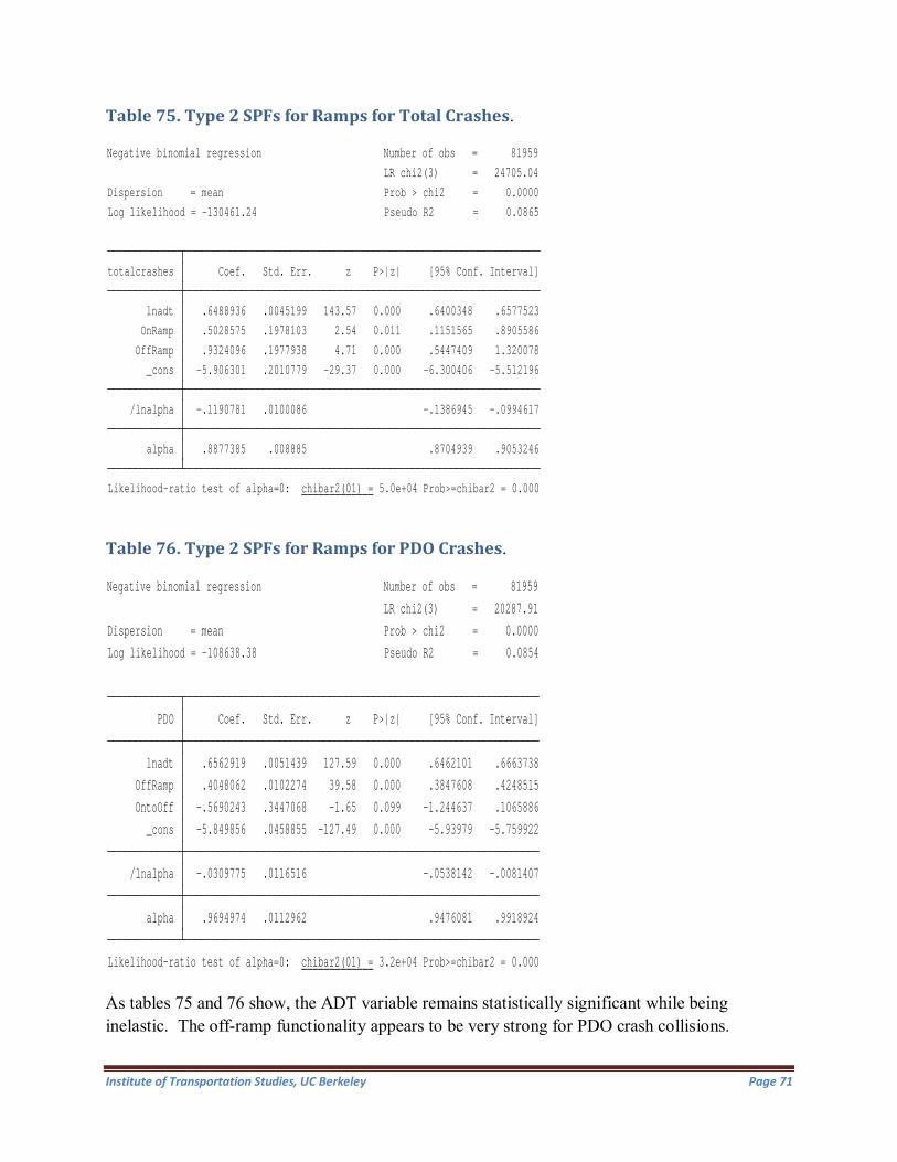
Table 75. Type 2 SPFs for Ramps for Total Crashes.

Table 76. Type 2 SPFs for Ramps for PDO Crashes.

As tables 75 and 76 show, the ADT variable remains statistically significant while being inelastic. The off-ramp functionality appears to be very strong for PDO crash collisions.

Likelihood-ratio test of alpha=0: chibar2(01) = 5.0e+04 Prob>=chibar2 = 0.000 alpha .8877385 .008885 .8704939 .9053246 /lnalpha -.1190781 .0100086 -.1386945 -.0994617 _cons -5.906301 .2010779 -29.37 0.000 -6.300406 -5.512196 OffRamp .9324096 .1977938 4.71 0.000 .5447409 1.320078 OnRamp .5028575 .1978103 2.54 0.011 .1151565 .8905586 lnadt .6488936 .0045199 143.57 0.000 .6400348 .6577523 totalcrashes Coef. Std. Err. z P>|z| [95% Conf. Interval]


Likelihood-ratio test of alpha=0: chibar2(01) = 3.2e+04 Prob>=chibar2 = 0.000 alpha .9694974 .0112962 .9476081 .9918924 /lnalpha -.0309775 .0116516 -.0538142 -.0081407 _cons -5.849856 .0458855 -127.49 0.000 -5.93979 -5.759922 OntoOff -.5690243 .3447068 -1.65 0.099 -1.244637 .1065886 OffRamp .4048062 .0102274 39.58 0.000 .3847608 .4248515 lnadt .6562919 .0051439 127.59 0.000 .6462101 .6663738 PDO Coef. Std. Err. z P>|z| [95% Conf. Interval]



Table 77. Type 2 SPFs for Ramps for Complaint of Pain Crashes.

Table 78. Type 2 SPFs for Ramps for Visible Injury Crashes.

As observed in table 78, the lack of geometric or non-ADT effects renders the visible injury type 2 SPF to be the same as the type 1 functional form. Complaint of pain however is influenced by both off and on ramp functionalities significantly.

Likelihood-ratio test of alpha=0: chibar2(01) = 6038.86 Prob>=chibar2 = 0.000 alpha 1.139117 .0249181 1.09131 1.189017 /lnalpha .1302532 .0218749 .087379 .1731273 _cons -8.129116 .5954194 -13.65 0.000 -9.296116 -6.962115 OffRamp 1.945977 .5923614 3.29 0.001 .7849695 3.106984 OnRamp 1.458803 .5923893 2.46 0.014 .2977417 2.619865 lnadt .6130114 .007551 81.18 0.000 .5982117 .627811 CP Coef. Std. Err. z P>|z| [95% Conf. Interval]


Likelihood-ratio test of alpha=0: chibar2(01) = 1448.69 Prob>=chibar2 = 0.000 alpha 1.133187 .0470723 1.044583 1.229307 /lnalpha .1250341 .0415398 .0436177 .2064506 _cons -6.743783 .0871005 -77.43 0.000 -6.914496 -6.573069 lnadt .5601032 .0096531 58.02 0.000 .5411833 .579023 Visible Coef. Std. Err. z P>|z| [95% Conf. Interval]



Table 79. Type 2 SPFs for Ramps for Severe Injury Crashes.

Table 80. Type 2 SPFs for Ramps for Fatal Injury Crashes.

Warning: convergence not achievedLikelihood-ratio test of alpha=0: chibar2(01) = 93.59 Prob>=chibar2 = 0.000 alpha 1.775995 .2876494 1.292935 2.439534 /lnalpha .574361 .1619652 .2569151 .891807 _cons -21.54248 . . . . . OffRamp 13.95382 .1942049 71.85 0.000 13.57318 14.33445 OnRamp 13.51002 .192909 70.03 0.000 13.13192 13.88811 lnadt .4721863 .0213066 22.16 0.000 .4304262 .5139464 Severe Coef. Std. Err. z P>|z| [95% Conf. Interval]


Warning: convergence not achievedLikelihood-ratio test of alpha=0: chibar2(01) = 23.70 Prob>=chibar2 = 0.000 alpha 2.426911 .8616429 1.210169 4.867005 /lnalpha .8866192 .3550369 .1907597 1.582479 _cons -24.15179 . . . . . OffRamp 14.56547 .3628027 40.15 0.000 13.85439 15.27655 OnRamp 14.02448 .36046 38.91 0.000 13.31799 14.73097 lnadt .566802 .0393387 14.41 0.000 .4896995 .6439045 Fatal Coef. Std. Err. z P>|z| [95% Conf. Interval]



As noticed in tables 79 and 80, model convergence was not achieved for severe and fatal injury collisions. This is most likely due to sparsity of crash counts at numerous ramp sites, due to the severity issue in question. It would therefore be reasonable to use the visible injury SPF as the default type 2 SPF for severe and fatal injury collisions for all ramps.

Tables 81-86 show the type 2 SPFs for the ramp metered subnetwork.

Table 81. Type 2 SPFs for Ramp Metered Locations for Total Crashes.

Table 81 shows the type 2 SPF for all total crashes for the ramp metered subnetwork. As is observed in the table, the number of lanes variable is the capacity related factor, while the connector, collector-distributor dummies capture the ramp geometry. The metered HOV dummy captures high occupancy effects. The number of lanes variable is not elastic, with an elasticity equal to 0.64. The ADT variable is also inelastic with an elasticity of 0.66.

Tables 82 and 83 show the type 2 SPFs for PDO and complaint of pain collisions for the ramp metered subnetwork. As can be seen in the tables, the statistical significance of the number of lanes and ramp geometry variables remains strong; however, the magnitudes are still in the inelastic range. The ADT variable continues to operate in the 0.70 elasticity range.

Likelihood-ratio test of alpha=0: chibar2(01) = 1654.30 Prob>=chibar2 = 0.000 alpha .627905 .028512 .5744372 .6863496 /lnalpha -.4653664 .0454081 -.5543646 -.3763682 _cons -5.705457 .2166421 -26.34 0.000 -6.130068 -5.280846 hovmeter -.3144367 .0528187 -5.95 0.000 -.4179593 -.210914 coldist -.5602787 .0958969 -5.84 0.000 -.748233 -.3723243 connector -.6020613 .0490803 -12.27 0.000 -.6982569 -.5058656 ofLanes .3281783 .0330524 9.93 0.000 .2633967 .3929599 lnadt .6641019 .0258991 25.64 0.000 .6133406 .7148631 TotalCrashes Coef. Std. Err. z P>|z| [95% Conf. Interval]



Table 82. Type 2 SPFs for Ramp Metered Locations for PDO Crashes.

Table 83. Type 2 SPFs for Ramp Metered Locations for Complaint of Pain Crashes.

Likelihood-ratio test of alpha=0: chibar2(01) = 1032.71 Prob>=chibar2 = 0.000 alpha .6697728 .0359225 .6029402 .7440134 /lnalpha -.4008168 .0536339 -.5059373 -.2956962 _cons -6.441491 .2494287 -25.82 0.000 -6.930362 -5.95262 hovmeter -.3084664 .0589081 -5.24 0.000 -.4239242 -.1930086 loop .0926589 .0467163 1.98 0.047 .0010966 .1842212 coldist -.4838733 .1065081 -4.54 0.000 -.6926253 -.2751213 connector -.5644273 .0565581 -9.98 0.000 -.6752791 -.4535754 ofLanes .3506135 .0371636 9.43 0.000 .2777741 .4234528 lnadt .6983929 .029612 23.58 0.000 .6403544 .7564313 PDO Coef. Std. Err. z P>|z| [95% Conf. Interval]


Likelihood-ratio test of alpha=0: chibar2(01) = 152.75 Prob>=chibar2 = 0.000 alpha .7555196 .0859232 .6045621 .9441709 /lnalpha -.2803495 .1137273 -.5032509 -.057448 _cons -7.313816 .3930371 -18.61 0.000 -8.084155 -6.543478 hovmeter -.2982878 .089538 -3.33 0.001 -.4737791 -.1227965 hook -.2982828 .1312783 -2.27 0.023 -.5555834 -.0409821 coldist -.7202889 .1703086 -4.23 0.000 -1.054088 -.3864901 connector -.9019132 .0938358 -9.61 0.000 -1.085828 -.7179983 ofLanes .2336579 .0558695 4.18 0.000 .1241556 .3431601 lnadt .6911846 .0467713 14.78 0.000 .5995145 .7828547 CP Coef. Std. Err. z P>|z| [95% Conf. Interval]



Table 84. Type 2 SPFs for Ramp Metered Locations for Visible Injury Crashes.

Table 85. Type 2 SPFs for Ramp Metered Locations for Severe Injury Crashes.

Likelihood-ratio test of alpha=0: chibar2(01) = 12.31 Prob>=chibar2 = 0.000 alpha .4816682 .165854 .2452741 .945898 /lnalpha -.7304997 .3443324 -1.405379 -.0556205 _cons -6.743953 .530995 -12.70 0.000 -7.784684 -5.703222 hovmeter -.430329 .1308323 -3.29 0.001 -.6867555 -.1739025 coldist -.7095001 .2712138 -2.62 0.009 -1.241069 -.1779308 connector -.3332938 .1177001 -2.83 0.005 -.5639818 -.1026058 ofLanes .3950526 .0788215 5.01 0.000 .2405653 .54954 lnadt .4862228 .0635088 7.66 0.000 .3617479 .6106978 Visible Coef. Std. Err. z P>|z| [95% Conf. Interval]


_cons -7.102819 1.147123 -6.19 0.000 -9.351139 -4.854499 hovmeter -.794243 .3797733 -2.09 0.036 -1.538585 -.049901 hook 1.170044 .2650076 4.42 0.000 .6506386 1.689449 ofLanes .3199715 .1911302 1.67 0.094 -.0546368 .6945798 lnadt .3154588 .1374426 2.30 0.022 .0460763 .5848414 Severe Coef. Std. Err. z P>|z| [95% Conf. Interval]

Log likelihood = -508.35183 Pseudo R2 = 0.0289 Prob > chi2 = 0.0000 LR chi2(4) = 30.24Poisson regression Number of obs = 4900


Table 86. Type 2 SPFs for Ramp Metered Locations for Fatal Injury Crashes.

As can be noticed in tables 85 and 86, type 2 SPFs for severe and fatal injuries follow the Poisson model. The fatal injury SPF is the same as the type 1 SPF with no geometric or traffic control effects found to be statistically significant.

Model Transferability and Predictions Three issues are relevant for post-estimation evaluation of the type 2 SPFs: Model checking via specification search, parameter stability via structural change tests, and predictive effectiveness via out of sample tests.

Specification: Several factors affect specification searches. Functional forms are usually tested in the safety community via cumulative residual plots. However, this method has significant limitations. It assumes apriori that the model contains numerous continuous variables, whose functional forms can be tested alternatively. In the current set of models that have been developed for this study, a majority of the variables are dummy types. Second, CURE plots do not address the issue of omitted variable bias. Omitted variable bias can arise when a variable that should be in the model is excluded, and the excluded variable share correlations with included variables in the model. When unobserved effects are significant in the models, the potential for omitted variable bias is non trivial and the CURE plot approach does not resolve the problem. It is important to note that including irrelevant variables in the models in order to enrich type 2 SPFs will cause inefficiency in the parameter estimates. Another issue that is significant in a multi-year panel of crash data such as the one used in this study is the effect of time. It has been noted repeatedly in several of the type 2 SPFs that year dummies are significant. In fact, years 2006-2010 appear to be negatively signed. This shows that year 2005 is a significant threshold for structural change. Further, when such time dummies are evaluated

_cons -8.760081 2.136095 -4.10 0.000 -12.94675 -4.573412 lnadt .4042716 .2396838 1.69 0.092 -.0655001 .8740432 Fatal Coef. Std. Err. z P>|z| [95% Conf. Interval]

Log likelihood = -203.58165 Pseudo R2 = 0.0076 Prob > chi2 = 0.0778 LR chi2(1) = 3.11Poisson regression Number of obs = 6080


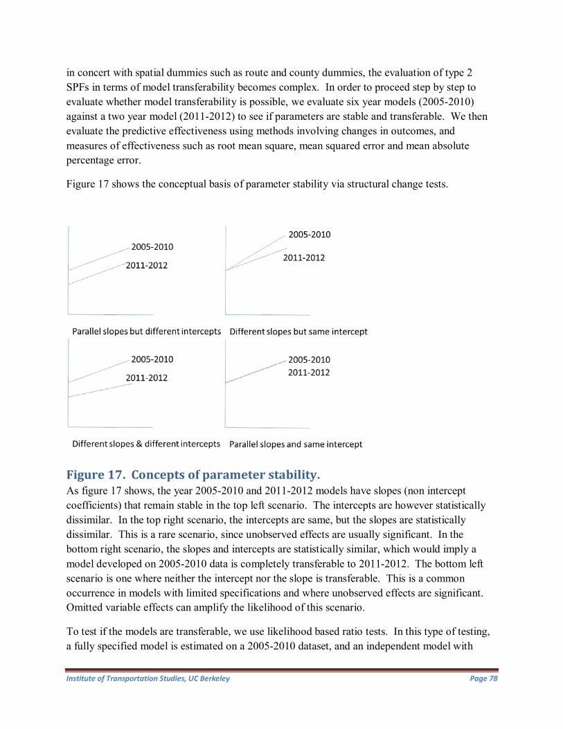
in concert with spatial dummies such as route and county dummies, the evaluation of type 2 SPFs in terms of model transferability becomes complex. In order to proceed step by step to evaluate whether model transferability is possible, we evaluate six year models (2005-2010) against a two year model (2011-2012) to see if parameters are stable and transferable. We then evaluate the predictive effectiveness using methods involving changes in outcomes, and measures of effectiveness such as root mean square, mean squared error and mean absolute percentage error.

Figure 17 shows the conceptual basis of parameter stability via structural change tests.

Figure 17. Concepts of parameter stability. As figure 17 shows, the year 2005-2010 and 2011-2012 models have slopes (non intercept coefficients) that remain stable in the top left scenario. The intercepts are however statistically dissimilar. In the top right scenario, the intercepts are same, but the slopes are statistically dissimilar. This is a rare scenario, since unobserved effects are usually significant. In the bottom right scenario, the slopes and intercepts are statistically similar, which would imply a model developed on 2005-2010 data is completely transferable to 2011-2012. The bottom left scenario is one where neither the intercept nor the slope is transferable. This is a common occurrence in models with limited specifications and where unobserved effects are significant. Omitted variable effects can amplify the likelihood of this scenario.

To test if the models are transferable, we use likelihood based ratio tests. In this type of testing, a fully specified model is estimated on a 2005-2010 dataset, and an independent model with


same exact specification is estimated on a 2011-2012 dataset. Then, a pooled model is estimated using the combined 2005-2012 dataset. The likelihood ratio evaluating the difference in likelihoods between the pooled model and the sum of the independent likelihoods is computed according to the following formula: 𝐿𝐿𝐿𝐿 = −(𝐿𝐿𝐿𝐿𝑝𝑝𝑝𝑝𝑝𝑝𝑙𝑙𝑝𝑝𝑝𝑝 − 𝐿𝐿𝐿𝐿2005−2010 − 𝐿𝐿𝐿𝐿2011−2012)~𝜒𝜒2. The LR statistic is chi-squared distributed with k degrees of freedom where k is the number of parameters being evaluated for a given model. If the computed chi-squared exceeds the chi-squared value for 99% confidence, then, this will indicate that the models are not transferable. This test does not indicate which parameters are not transferable, it indicates if the model as a whole is transferable.

Architecture of the LR test: Since we have 10 SPF classes, and two data periods (2005-2010 versus 2011-2012), we need to estimate a pooled model and two unrestricted models, involving six injury classes including total, PDO, complaint of pain, visible, severe and fatal types. Thus, we have 18 models to be evaluated for each SPF class, resulting in a total of 180 LR tests.

Tables 87-92 shows the results of completed transferability tests.

Table 87. Rural 2-Lane Transferability Test by Severity.

As table 87 shows, with the exception of PDO type 2 SPFs, none of the other SPFs are transferable at the 99% confidence level. The computed LRs exceed the threshold values. Table 88 shows LR tests for rural 4-lane roadways, and it will be noted that the degree to which the computed LRs exceed the threshold values is far greater than that seen in table 87. This shows that the effect of unobservable is greater in rural 4-lane roadway datasets, and specification searches need to incorporate alignment data to reduce the effect of unobservables. Tables 89 and 90 on the other hand show conformant results for rural 4-plus-lane and rural multilane undivided datasets, where all models appear transferable at the 99% confidence level. Clearly, the heterogeneity in four-lane rural datasets appears to indicate a need for richer specifications, and to a lesser degree in rural two-lane datasets as well. The LR conformity of rural multilane undivided models is very strong, and it can be said that the parameter transferability in these type 2 SPFs as well as the rural 4-plus-lane models is supported.


Table 88. Rural 4-Lane Transferability Test by Severity.

Table 89. Rural 4-Plus-Lane Transferability Test by Severity.

Table 90. Rural Multi-Lane Undivided Transferability Test by Severity.


Tables 91-96 show LR tests for urban roadways. As seen in the tables, the urban 2-lane, urban 4-lane type 2 SPF and 5-6-7-lane type 2 are not transferable.

Table 91. Urban Two-Lane Transferability Test by Severity.

Table 92. Urban Four-Lane Transferability Test by Severity.

Table 93. Urban Five-Six-Seven-Lane Transferability Test by Severity.


Table 94. Urban Eight-Plus-Lane Transferability Test by Severity.

Table 95. Urban Multi-Lane Undivided Transferability Test by Severity.

Table 96. Urban Multi-Lane Divided Transferability Test by Severity.


Tables 97-98 show the out of sample prediction tests using estimated type 2 SPF predictions (from 2005-2010) of 2011 data.

Table 97. Prediction Measures of Effectiveness for 2011 Out of Estimation Sample Predictions by Rural SPF Class.

Type 1 SPF Type 2 SPF SPF Class Outcome MAD MAPE RMSE MAD MAPE RMSE

Total 0.363 182.926 0.814 0.329 182.538 0.618 PDO 0.196 191.448 0.241 0.187 191.345 0.205

2-Lane CPAIN 0.082 198.104 0.061 0.078 197.975 0.055 VISIBLE 0.112 197.173 0.102 0.105 197.068 0.090 SEVERE 0.048 199.393 0.032 0.046 199.277 0.030 FATALITY 0.017 199.877 0.009 0.017 199.846 0.009 Total 0.649 172.971 4.608 0.588 172.142 4.948 PDO 0.415 181.954 1.862 0.386 181.432 2.346


4+Lane CPAIN 0.785 183.312 0.933 0.431 181.822 0.863 VISIBLE 0.253 184.062 0.259 0.256 183.679 0.269 SEVERE 0.061 198.471 0.037 0.060 198.255 0.037 FATALITY 0.018 199.893 0.009 0.018 193.519 0.009 Total 0.351 173.436 0.315 0.350 173.862 0.308 PDO 0.256 184.542 0.172 0.252 184.553 0.173

Multi-Lane CPAIN 0.072 199.312 0.038 0.070 199.363 0.036 Undivided VISIBLE 0.085 197.832 0.049 0.077 196.931 0.041

SEVERE 0.065 199.260 0.051 0.064 173.093 0.051 FATALITY 0.033 199.619 0.017 0.032 159.564 0.017

The measures of effectiveness are useful due to their particular implications in terms of predictive capability out of sample. Mean absolute deviation is meaningful when cost of forecast error is proportional to the absolute size of the error. Mean absolute percent error is meaningful when cost of error is related to percent than numerical size of error. Mean squared error (and root mean squared error) are meaningful in a quadratic loss function manner – they tend to weight large errors heavily compared to small errors.

By these definitions, type 2 SPFs are comparatively better than type 1 SPFs in both 2011 and 2012 out of sample predictions.


Table 98. Prediction Measures of Effectiveness for 2011 Out of Estimation Sample Predictions by Urban SPF Class.


Total 0.985 171.631 50.621 0.834 170.642 29.606 PDO 0.612 181.724 17.342 0.527 181.090 10.138



5,6,&7-Lane

CPAIN 1.225 153.713 8.739 1.129 152.579 7.567

VISIBLE 0.502 171.079 1.267 0.485 170.840 1.082 SEVERE 0.129 193.943 0.100 0.128 193.020 0.098 FATALITY 0.062 198.606 0.043 0.058 178.374 0.045 Total 7.608 89.172 219.397 7.250 87.956 201.322 PDO 5.599 98.499 120.225 5.403 97.552 113.398


Multi-Lane CPAIN 0.492 187.118 1.831 0.378 186.024 0.740 Divided VISIBLE 0.179 194.777 0.202 0.170 194.774 0.167

SEVERE 0.045 199.283 0.027 0.045 199.313 0.026 FATALITY 0.023 199.710 0.013 0.023 199.711 0.013

Tables 99 and 100 show the out of sample prediction measures of effectiveness for year 2012 datasets. The patterns observed are similar to the ones shown in tables 97-98.


Table 99. Prediction Measures of Effectiveness for 2012 Out of Estimation Sample Predictions by Rural SPF Class.


Total 0.285 186.925 0.441 0.267 186.733 0.354 PDO 0.203 191.965 0.241 0.189 192.088 0.201





SEVERE 0.095 197.876 0.134 0.036 187.786 0.026 FATALITY 0.017 199.233 0.034 0.024 198.763 0.029


Table 100. Prediction Measures of Effectiveness for 2012 Out of Estimation Sample Predictions by Urban SPF Class.


Total 0.772 176.881 28.989 0.652 175.569 15.568 PDO 0.562 182.440 13.759 0.492 181.999 7.912



5,6,& CPAIN 0.728 168.154 2.894 0.683 167.410 2.440 7-Lane VISIBLE 0.350 181.174 0.633 0.344 181.085 0.579

SEVERE 0.092 196.763 0.064 0.093 196.807 0.064 FATALITY 0.053 198.857 0.032 0.052 198.791 0.032 Total 6.401 91.771 155.451 6.228 90.730 157.301 PDO 5.311 97.281 106.661 5.189 96.332 111.583


Multi-Lane CPAIN 0.248 193.240 0.357 0.217 187.978 0.283 Divided VISIBLE 0.109 197.396 0.098 0.104 197.327 0.088

SEVERE 0.032 199.632 0.017 0.032 199.658 0.017 FATALITY 0.016 199.873 0.009 0.016 199.874 0.009 Total 0.944 174.736 6.700 0.799 174.132 4.267 PDO 0.692 181.997 3.595 0.580 176.802 2.123


SEVERE 0.016 199.886 0.008 0.016 170.016 0.008 FATALITY 0.026 199.840 0.013 0.024 162.126 0.013

Conclusions and Recommendations An evaluation of the type 1 and type 2 SPFs for roadway segments indicates that segment length based on homogeneous geometry results in a large proportion of segments under the length of 0.1 mile. This implies that network screening should be conducted at the 0.1-mile interval, instead of at higher intervals. It is also our finding that re-defining segment lengths to minimize sensitivity to network screening outcomes from Safety Analyst is a complex decision making


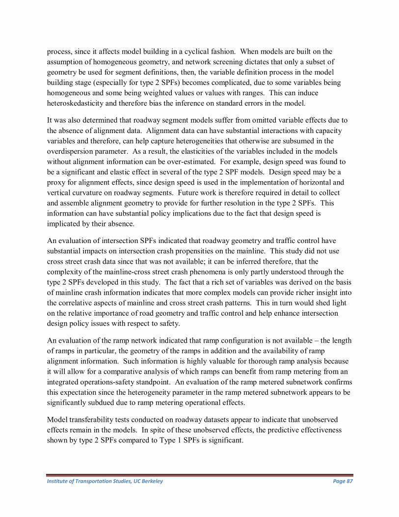
process, since it affects model building in a cyclical fashion. When models are built on the assumption of homogeneous geometry, and network screening dictates that only a subset of geometry be used for segment definitions, then, the variable definition process in the model building stage (especially for type 2 SPFs) becomes complicated, due to some variables being homogeneous and some being weighted values or values with ranges. This can induce heteroskedasticity and therefore bias the inference on standard errors in the model.

It was also determined that roadway segment models suffer from omitted variable effects due to the absence of alignment data. Alignment data can have substantial interactions with capacity variables and therefore, can help capture heterogeneities that otherwise are subsumed in the overdispersion parameter. As a result, the elasticities of the variables included in the models without alignment information can be over-estimated. For example, design speed was found to be a significant and elastic effect in several of the type 2 SPF models. Design speed may be a proxy for alignment effects, since design speed is used in the implementation of horizontal and vertical curvature on roadway segments. Future work is therefore required in detail to collect and assemble alignment geometry to provide for further resolution in the type 2 SPFs. This information can have substantial policy implications due to the fact that design speed is implicated by their absence.

An evaluation of intersection SPFs indicated that roadway geometry and traffic control have substantial impacts on intersection crash propensities on the mainline. This study did not use cross street crash data since that was not available; it can be inferred therefore, that the complexity of the mainline-cross street crash phenomena is only partly understood through the type 2 SPFs developed in this study. The fact that a rich set of variables was derived on the basis of mainline crash information indicates that more complex models can provide richer insight into the correlative aspects of mainline and cross street crash patterns. This in turn would shed light on the relative importance of road geometry and traffic control and help enhance intersection design policy issues with respect to safety.

An evaluation of the ramp network indicated that ramp configuration is not available – the length of ramps in particular, the geometry of the ramps in addition and the availability of ramp alignment information. Such information is highly valuable for thorough ramp analysis because it will allow for a comparative analysis of which ramps can benefit from ramp metering from an integrated operations-safety standpoint. An evaluation of the ramp metered subnetwork confirms this expectation since the heterogeneity parameter in the ramp metered subnetwork appears to be significantly subdued due to ramp metering operational effects.

Model transferability tests conducted on roadway datasets appear to indicate that unobserved effects remain in the models. In spite of these unobserved effects, the predictive effectiveness shown by type 2 SPFs compared to Type 1 SPFs is significant.


Table 101. Model Transferability with Varying Panels of Years.

Rural Urban SPF Class Outcome 2006-2010

Model Transferable?

2007-10 Model

Transferable?

2008-2010 Model

Transferable

2006-2010 Model

Transferable?

2007-10 Model

Transferable?

2008-2010 Model

Transferable Total No No No No No No PDO Yes No No No No No

2-Lane CPAIN No No No No No No VISIBLE No No No No No No SEVERE No No No No No Yes FATALITY No Yes Yes No No No Total No No No No No No PDO No No No No No Yes

4-Lane CPAIN No No No No No No VISIBLE No No No No No No SEVERE No No No No No No FATALITY No Yes Yes No No Yes Total Yes Yes Yes PDO Yes Yes Yes

4+Lane CPAIN Yes Yes Yes VISIBLE Yes Yes Yes SEVERE Yes Yes Yes FATALITY Yes Yes Yes Total Yes Yes Yes No No No PDO Yes Yes Yes No No No

Multi-Lane

CPAIN Yes Yes Yes No No Yes

Undivided VISIBLE Yes Yes Yes No Yes Yes SEVERE Yes Yes Yes Yes Yes Yes FATALITY Yes Yes Yes Yes Yes Yes Total No No No PDO No No No

5,6,7-Lane

CPAIN No No No

VISIBLE No No No SEVERE No No No FATALITY No No Yes Total Yes No No PDO No No Yes

8-Lane CPAIN No No No VISIBLE No No No SEVERE No No No FATALITY No Yes Yes Total No No No

PDO No No No

Multi-Lane

CPAIN No No No

Divided VISIBLE No No No SEVERE Yes Yes Yes FATALITY Yes Yes Yes


Environmental data is very challenging to collect on a statewide level, especially when one wishes to collect pavement level information. Economic effects at the SPF class level or route level are pose enormous data collection challenges. While it can be theorized that economic effects can influence driving exposure, as well as trip making behavior (for example, making more discretionary trips out of the home such as recreational and entertainment related), measuring aggregate manifestations of such effects at the route level or even district level is close to impossible. These unobserved effects can remain for several years. In the absence of environmental and economic data, consistent alignment information will mitigate the unobserved effects considerably, especially in terms of horizontal and vertical curvature information. In urban environments especially, alignment information can be critical due to the more frequent interactions between traffic flow and roadway geometry. Table 101 further emphasizes this point through the illustration of the longitudinal change in the likelihood ratio tests. In summary, on the basis of both transferability and predictive measures of effectiveness, it can be said that Type 2 SPFs offer far more effective decision making bases for identifying high collision concentrations than Type 1 SPFs.


All-Districts: Urban Multilane Divided SPF 2 –Total Fatalities

All-Districts: Urban Multilane Divided SPF 2 – Total Injuries

Horaal - exit fro• iterations. Exit s t atus=O .

+---------------------------------------------+ Negative Binoaial Regression Kaxiaua Likelihood Estiaates Kadel estiaated : Kay 13. 2014 Dependent variable Weighting variable Huaber of observations Iterations coaplet ed Log likelihood function Nuaber of paraaeters Info. Criterion : AIC

Finite Saaple : AIC = Info. Criterion : BIC = Info. Criterion : HQIC = Restricted log likelihood Kc Fadden Pseudo R-squared Chi squared Degrees of freedoa Prob[ChiSqd > value] = KegBin fora 2; Psi(i) = theta

at 08:59 : 14PK. TOTAL IN

None 2150

3 2 - 3146.73 3

2 2 2 . 94766 2 . 94788 3 . 00571 2 . 96890

-4225.331 . 2552694 2157.196

1 . 0000000

+---------------------------------------------+ +--------+--------------+----------------+--------+--------+----------+ IVariablel Coefficient I Standard Error lb/St.Er . IP[IZI >z]l Kean of XI +--------+--------------+----------------+--------+--------+----------+

Constant -6.68984854 .82381284 -8.121 .0000 LOGADT 1.01634728 .07207555 14.101 .0000 LOGLK 1.00000000 ..... . (Fixed Paraaeter) ..... . . LTLAKES .20432446 .10121756 2.019 .0435 LT_IS_VI .09608650 .02378363 4.040 .0001 RT_IS_VI -.10379896 .03037566 -3.41 7 .0006 DES_SP -.0 3244610 .00409757 -7.918 .0000 KETVTL -.5 3981933 .11529251 -4.682 .0000 KEPAVE -.35452651 .10720673 -3. 30 7 .0009 KEKPAVE -.36426485 .13165506 -2. 76 7 .0057 KESTRUC -1.7 2971530 .64801248 -2.669 .00 76 KEBRAIL 1.50259509 .59192446 2.538 .0111 KEKOBARR .38884648 .19103362 2.035 .0418 SCL -.8 2829526 .15009363 -5.519 .0000 VEK 1.17072277 .38958826 3.005 .00 27 RIV -.4 2661215 .15390131 -2. 772 .0056 SBD .51618293 .13935782 3. 704 .0002 KER -.64612442 .25543134 -2.530 .0114 IKP -.65401482 .14402290 -4.541 .0000 RT33 -1.61030294 .47997442 -3. 355 .0008 RT18 -.76625480 .22433629 -3.416 .0006 RT 7 4 .96118513 .21153978 4.544 .0000

---------+Dispersion paraaeter for count data aodel Alpha I 1.50340641 .08624217 17.432 .0000

9.95892811

2.15767442 2.11302326 2.14883721 55 . 0162791

.18418605

. 26000000

. 27255814

.0790697 7

.08139535

.84558140

.07581395

.03302326

.0948837 2

.08976744

.04279070

.10790698

.03116279

.02976744

.03860465

All-Districts: Urban Multilane Divided SPF 2 – Total Noninjuries

Noraal exit fro• iterations. Exit status=O.

+---------------------------------------------+ Negative Binoaial Regression Kaxiaua Likelihood Estiaates Kadel estiaated: Kay 13. 2014 Dependent variable Veighting variable Huaber of observations Iterations coapleted Log likelihood function Hu•ber of paraaeters Info. Criterion: AIC

Finite Saaple: AIC = Info. Criterion: BIC = Info. Criterion:HQIC = Restricted log likelihood KcFadden Pseudo R-squared Chi squared Degrees of freedoa Prob[ChiSqd > value] = HegBin fora 2; Psi(i) = theta

at 09:04 : 18PK. TOTALHI

Hone 2146

32 -3124.392

22 2.93233 2.93255 2.99047 2.95360

-4196.906 .2555487 2145.028

1 .0000000

+---------------------------------------------+ +--------+--------------+----------------+--------+--------+----------+ IVariablel Coefficient I Standard Error lb/St.Er . IP[IZI>z]l Kean of XI +--------+--------------+----------------+--------+--------+----------+ Constant -6.79627324 . 82258213 LOGADT 1.02895535 . 07202110 LOGLH 1.00000000 .... .. (Fixed LTLAHES .20462452 . 10120727 LT_IS_VI .09641763 . 02366126 RT_IS_VI -.10679965 . 03037240 DES_SP -.03300736 . 00410671 KETVTL -.56033415 . 11610620 KEPAVE -.35904379 . 10732198 KEHPAVE -.35551370 . 13249084 KESTRUC -1.73799328 . 64923643 KEBRAIL 1.52499364 . 59278596 KEHOBARR .39115749 . 19130100 SCL -.83362501 . 15089729 VEH 1.17648188 . 38777743 RIV -.43128692 . 15536964 SBD .52663510 . 13920890 KER -.63376536 . 25557518 IKP -.63901699 . 14447489 RT33 -1.59965413 . 47976875 RT18 -.73493626 . 22809227 RT74 .96888080 . 21469348

---------+Dispersion paraaeter for count Alpha I 1.51171645 . 08710103

-8.262 . 0000 14.287 .0000

Paraaeter) .. .... . 2.022 .0432 4.075 .0000

-3.516 . 0004 -8.037 . 0000 -4.826 . 0000 -3.345 .0008 -2.683 . 0073 -2.677 . 0074

2.573 .0101 2.045 .0409

-5.524 . 0000 3.034 .0024

-2.776 . 0055 3.783 .0002

-2.480 . 0131 -4.423 . 0000 -3.334 .0009 -3.222 . 0013

4.513 .0000 data aodel

17.356 .0000

9.95899822

2.15796831 2.11230196 2.14818267 55.0046598

.18406337

.26048462

.27213420

.07921715

.08154706

.84529357

.07548928

.03308481

.09506058

.08946878

.04287046

.10764212

.03122088

.02935694

.03867661

All-Districts: Urban Four-lane SPF 1 –Total Noninjuries

All-Districts: Urban Four-lane SPF 1 –Total Fatalities

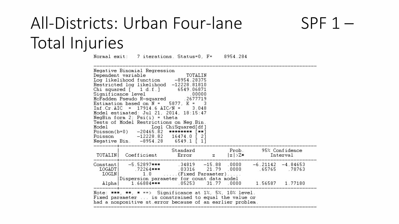
All-Districts: Urban Four-lane SPF 1 –Total Injuries

All-Districts: Urban Four-lane SPF 2 –Total Fatalities

All-Districts: Urban Four-lane SPF 2 – Total Injuries Normal exit: 34 iterations. Status=O, F=

Negative Binomial Regression Dependent variable TOTALIN Log likelihood function -8662.63453 Restricted log likelihood -10991.75057 Chi squared [ 1 d.f.] 4658.23208 Significance level .00000 McFadden Pseudo R-squared .2118967 Estimation based on N = 5877. K 27 Inf.Cr.AIC 17379.3 AIC/N = 2.957 Model estimated: Jul 22. 2014. 04:04:12 NegBin form 2; Psi(i) = theta Tests of Model Restrictions on Neg.Bin. Model Log! ChiSquared[df] Poisson(b=O) -20465.82 ******** [**] Poisson -10991.75 18948.1 [26] Negative Bin. -8662.63 4658.2 [ 1]

8662. 6351

--------+--------------------------------------------------------------------1 Standard Prob. 95% Confidence

TOTALINI Coefficient Error z lzi>Z* Interval --------+--------------------------------------------------------------------Constant -6.56045*** .42718 -15.36 .0000 -7.39771 -5.72318

LOGADT . 99310*** . 03831 25. 92 . 0000 . 91802 1. 06819 LOGLN 1. 0 ..... (Fixed Parameter).

DES SP -.02752*** .00264 -10.41 .0000 METYTL -.35301*** .12916 -2.73 .0063

RT15 -. 53568*** .18915 -2. 83 . 0046 RT210 -. 50410** . 22970 -2 .19 . 0282 RT105 . 55057** . 25897 2 .13 . 0335

RT2 -1. 44332*** . 24 710 -5. 84 . 0000 RT135 1.10340* . 56363 1. 96 . 0503

RT13 . 86037*** . 26940 3 .19 . 0014 RT99 -. 23920*** . 06148 -3. 89 . 0001

RT101 -. 56434*** . 06644 -8.49 . 0000 LA .39219*** .08636 4.54 .0000

SON . 40660*** . 09321 4. 36 . 0000 ALA -.70414*** .12584 -5.60 .0000 YUB -.73144*** .24136 -3.03 .0024

MECONCG -.49184*** .13223 -3.72 .0002 MEBEAM . 71217*** .16853 4. 23 . 0000

MESTRUC -.66431*** .11414 -5.82 .0000 MEDIT -1.96983** .78866 -2.50 .0125 MESGR -.74715*** .17316 -4.31 .0000

MENPAVE -.54051*** .09144 -5.91 .0000 MEPAVE -.59115*** .08839 -6.69 .0000

MEST -.35398*** .10306 -3.43 .0006 MED WI -.00651*** .00115 -5.64 .0000

LTLANES . 34827*** . 06935 5. 02 . 0000 Dispersion parameter for count data model

Alpha 1.28092*** .04329 29.59 .0000

-. 03271 -.60616 -.90640 -.95430

.04301 -1.92762 -.00129

.33236 -.35970 -.69457

.22293

.22391 -.95078

-1.20450 -.75100

.38186 -.88802

-3.51557 -1.08654 -. 71972 -.76438 -.55597 -. 00877

.21234

1.19608

-.02234 -.09987 -.16495 -.05390 1.05813 -.95901 2.20809 1.38838 -.11871 -. 43411

.56144

. 58928 -.45750 -.25838 -.23267 1.04248 -.44060 -.42409 -.40777 -.36129 -.41791 -.15200 -.00425

.48420

1.36577 --------+--------------------------------------------------------------------

All-Districts: Urban Four-lane SPF 2 – Total NoninjuriesNormal exit: 34 iterations. Status=O, F=

Negative Binomial Regression Dependent variable TOTALN: Log likelihood function -8596.36938 Restricted log likelihood -10888.80273 Chi squared [ 1 d.f.] 4584.8667: Significance level .00000 McFadden Pseudo R-squared .2105313 Estimation based on N = 5863. K 2? Inf.Cr.AIC 17246.7 AIC/N = 2.942 Model estimated: Jul 22. 2014. 04:05:2l NegBin form 2; Psi(i) = theta Tests of Model Restrictions on Neg.Bin Model Log! ChiSquared[df] Poisson(b=O) -20163.13 ******** [**] Poisson -10888.80 18548.7 [26] Negative Bin. -8596.37 4584.9 [ 1]

8596.369


TOTALNI] Coefficient Error z ]z]>Z* Interval --------+--------------------------------------------------------------------Constant -6. 59800*** . 42836 -15.40 . 0000 -7.43757 -5.75842

LOGADT 1. 00071*** . 03851 25. 99 . 0000 . 92523 1. 07619 LOGLN 1. 0 ..... (Fixed Parameter).

DES SP -.02845*** .00266 -10.70 .0000 METWTL -.36681*** .12965 -2.83 .0047

RT15 -. 55556*** .18826 -2. 95 . 0032 RT210 -. 4 7269** . 23630 -2. 00 . 0455 RT105 . 57536** . 25924 2. 22 . 0265

RT2 -1. 40317*** . 24 734 -5. 6 7 . 0000 RT135 1.11166** . 56401 1. 97 . 0487

RT13 . 87752*** . 26960 3. 25 . 0011 RT99 -. 24479*** . 06189 -3.96 . 0001

RT101 -. 55982*** . 06654 -8.41 . 0000 LA .36427*** .08757 4.16 .0000

SON . 40940*** . 09301 4. 40 . 0000 ALA -. 70664*** .12573 -5. 62 . 0000 YUB -.72551*** .24100 -3.01 .0026

MECONCG -.47797*** .13341 -3.58 .0003 MEBEAM .71961*** .16879 4.26 .0000

MESTRUC -.65673*** .11399 -5.76 .0000 MEDIT -1. 95985** . 78722 -2.49 . 0128 MESGR -.77110*** .17232 -4.47 .0000

MENPAVE -.54013*** .09120 -5.92 .0000 MEPAVE -.59374*** .08826 -6.73 .0000

MEST -.36092*** .10307 -3.50 .0005 MED YI -.00637*** .00116 -5.50 .0000

LTLANES .34916*** .06993 4.99 .0000 Dispersion parameter for count data model

-.03367 -.62092 -.92455 -.93584

.06726 -1.88794

.00621

.34911 -.36610 -.69023

.19264

. 22711 -.95307

-1.19786 -.73945

.38878 -. 88014

-3.50278 -1.10883 -. 71888 -.76674 -.56294 -.00864

. 21211

-.02324 -.11270 -.18658 -.00954 1.08347 -.91841 2.21711 1.40593 -.12348 -.42941

.53590

.59169 -.46020 -.25316 -.21650 1.05044 -.43332 -.41692 -.43337 -.36139 -.42075 -.15890 -.00410

.48621

Alpha 1. 27978*** . 04345 29.45 . 0000 1.19461 1. 36495 --------+--------------------------------------------------------------------

All-Districts: Urban Five, Six, and Seven-lane SPF 1 – Total Noninjuries

Normal exit: 8 iterations. Status=O, F=

Negative Binomial Regression Dependent variable TOTALNI Log likelihood function -7185.64728 Restricted log likelihood -10077.93490 Chi squared [ 1 d.f.] 5784.57523 Significance level .00000 McFadden Pseudo R-squared .2869921 Estimation based on N = 4053. K = 3 Inf.Cr.AIC = 14377.3 AIC/N = 3.547 Model estimated: Jul 22. 2014. 14:59:14 NegBin form 2; Psi(i) = theta Tests of Model Restrictions on Neg.Bin. Model Log! ChiSquared[df] Poisson(b=O) -20626.43 ******** [**] Poisson -10077.93 21097.0 [ 2] Negative Bin. -7185.65 5784.6 [ 1]

7185.647


TOTALNII Coefficient Error z lzi>Z* Interval --------+--------------------------------------------------------------------Constant! -7.05513*** .32979 -21.39 .0000 -7.70151 -6.40876

LOGADT I . 86631*** . 02911 29. 76 . 0000 . 80925 . 92338 LOGLN I 1. 0 ..... (Fixed Parameter).

!Dispersion parameter for count data model Alpha I 1. 29028*** . 04 731 27. 27 . oooo 1.19755 1. 38301

--------+--------------------------------------------------------------------Note: ***, **, * ==> Significance at 1%, 5%, 10% level. Fixed parameter is constrained to equal the value or had a nonpositive st.error because of an earlier problem.

All-Districts: Urban Five, Six, and Seven-lane SPF 1 – Total Fatalities


Negative Binomial Regression Dependent variable TOTALFA Log likelihood function -573.68573 Restricted log likelihood -582.37093 Chi squared [ 1 d.f.] 17.37040 Significance level .00003 McFadden Pseudo R-squared .0149135 Estimation based on N = 4065. K = 3 Inf.Cr.AIC = 1153.4 AIC/N = .284 Model estimated: Jul 22. 2014. 14:59:26 NegBin form 2; Psi(i) = theta Tests of Model Restrictions on Neg.Bin. Model Log! ChiSquared[df] Poisson(b=O) -710.47 ******** [**] Poisson -582.37 256.2 [ 2] Negative Bin. -573.69 17.4 [ 1]

573.6857


TOTALFAI Coefficient Error z lzi>Z* Interval --------+--------------------------------------------------------------------Constant! -9.40974*** 2.20034 -4.28 .0000 -13.72232 -5.09715

LOGADTI . 67428*** .19238 3. 50 . 0005 . 29722 1. 05134 LOGLN I 1. 0 ..... (Fixed Parameter).

!Dispersion parameter for count data model Alpha I 1. 80900*** . 46702 3. 87 . 0001 . 89366 2. 72434


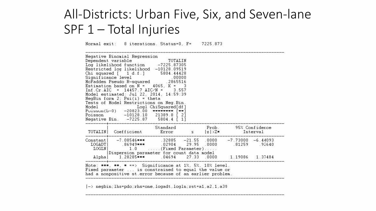
All-Districts: Urban Five, Six, and Seven-lane SPF 1 – Total Injuries


Negative Binoaial Regression Dependent variable TOTALIN Log likelihood function -7225.87305 Restricted log likelihood -10128.09519 Chi squared [ 1 d.f.] 5804.44428 Significance level .00000 McFadden Pseudo R-squared .2865516 Estimation based on N = 4065. K = 3 Inf.Cr.AIC = 14457.7 AIC/N = 3.557 Model estimated: Jul 22. 2014. 14:59:39 NegBin form 2; Psi(i) = theta Tests of Model Restrictions on Neg.Bin. Model Log! ChiSquared[df] Pu.it::>t::>uu(L-0) -20823.00 """""""" [••] Poisson -10128.10 21389.8 [ 2] Negative Bin. -7225.87 5804.4 [ 1]

7225.873

--------+--------------------------------------------------------------------1 Standard Prob. 95% Con£ ider.ce

TOTALINI Coefficient Error z lzi>Z* Interval --------+--------------------------------------------------------------------Constant I -7. 08546*** . 32885 -21.55 . 0000 -7. 73000 -6. 44093

LOGADTI . 86949*** . 02904 29.95 . 0000 . 81259 . 9<640 LOGLN I 1. 0 ..... (Fixed Parameter).

!Dispersion parameter for count data model Alpha I 1. 28285*** . 04694 27.33 . oooo 1.19086 1. 3/484


1-> negbin;lhs=pdo;rhs=one.logadt.logln;rst=a1.a2.1.a3$

All-Districts: Urban Five, Six, and Seven-lane SPF 2 – Total NoninjuriesNormal exit: 34 iterations. Status=O, F=

Negative Binomial Regression Dependent variable TOTALNI Log likelihood function -7025.83202 Restricted log likelihood -9269.03317 Chi squared [ 1 d.f.] 4486.40229 Significance level .00000 McFadden Pseudo R-squared .2420103 Estimation based on N • 4053. K • 25 Inf.Cr.AIC 14101.7 AIC/N • 3.479 Model estimated: Jul 22. 2014. 19:01:22 NegBin form 2; Psi(i) • theta Tests of Model Restrictions on Neg.Bin. Model Log! ChiSquared[df] Poisson(b•O) -20626.43 ******** [**] Poisson -9269.03 22714.8 [24] Negative Bin. -7025.83 4486.4 [ 1]

7025.832


TOTALNII Coefficient Error z lzi>Z* Interval --------+--------------------------------------------------------------------Constant -7.33725*** .40952 -17.92 .0000 -8.13988 -6.53461

LOGADT 1. 024 73*** . 03954 25. 92 . 0000 . 94 723 1.10223 LOGLN 1. 0 ..... (Fixed Parameter).

DES SP -. 01854*** . 00368 -5. 04 . 0000 LNOSPEC - .19950*** . 05571 -3. 58 . 0003

SF . 54909*** .15568 3. 53 . 0004 SCL -.19391** .09225 -2.10 .0356 SLO -.70670** .35549 -1.99 .0468

MEST -1.41225*** .47394 -2.98 .0029 MED WI -. 00519*** . 00080 -6. 4 7 . 0000

RLTR . 33623*** .11779 2. 85 . 0043 PLA -. 78199*** . 22703 -3.44 . 0006 sur 1. 03660** . 40256 2. 57 . 0100 FRE . 59995*** .10458 5. 74 . 0000

LA . 28544*** . 06489 4. 40 . 0000 RT65 1. 40387*** . 28656 4. 90 . 0000 RT44 2. 50060*** . 46883 5. 33 . 0000 RT24 -. 71925*** . 23814 -3. 02 . 0025 RT14 -. 46928*** .14471 -3.24 . 0012

RT178 1. 04453*** . 25126 4.16 . 0000 RT23 . 90750** . 38512 2. 36 . 0185 RT71 -. 776 70** . 35962 -2 .16 . 0308

RT215 . 60925*** .11561 5. 27 . 0000 RT905 -1. 50059*** . 50570 -2. 97 . 0030 RT261 -1. 05529** . 4 7353 -2. 23 . 0258

Dispersion parameter for count data model

-.02574 -.30870

.24395 -.37472

-1.40344 -2.34115 -. 00677

.10537 -1.22697

.24759

.39498

.15826

.84222 1.58171

-1.18600 -.75291

.55207

.15268 -1.48154

.38265 -2.49174 -1.98340

-. 01133 -.09031

.85422 -.01309 -.00995 -.48335 -.00362

.56709 -.33701 1.82562

.80492

. 41262 1.96551 3.41948 -.25250 -.18564 1.53700 1.66232 -. 07185

.83585 -.50944 -.12718

Alpha 1. 06987*** . 04250 25.17 . 0000 . 98657 1.15317 --------+--------------------------------------------------------------------

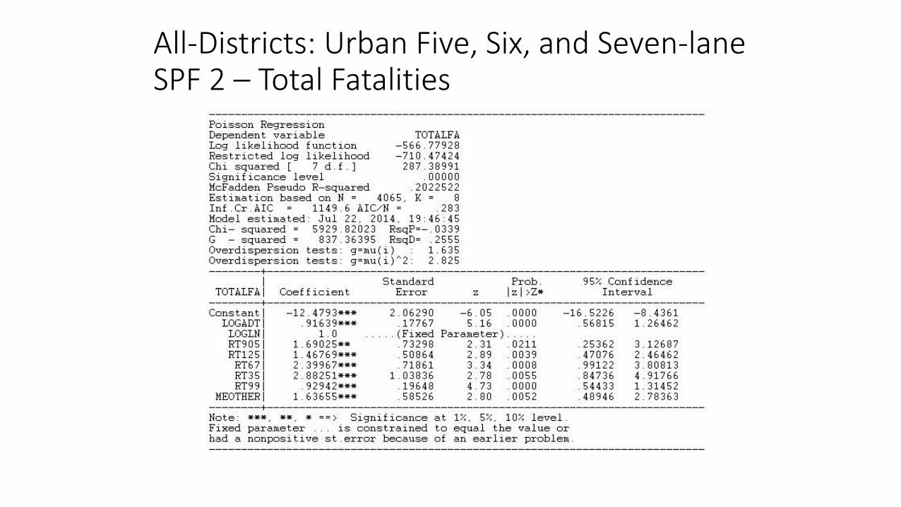
All-Districts: Urban Five, Six, and Seven-lane SPF 2 – Total Fatalities

Poisson Regression Dependent variable TOTALFA Log likelihood function -566.77928 Restricted log likelihood -710.47424 Chi squared [ 7 d.f.] 287.38991 Significance level .00000 McFadden Pseudo R-squared .2022522 Estimation based on N = 4065. K = 8 Inf.Cr.AIC = 1149.6 AIC/N = .283 Model estimated: Jul 22. 2014. 19:46:45 Chi- squared= 5929.82023 RsqP=-.0339 G -squared= 837.36395 RsqD= .2555 Overdispersion tests: g=mu(i) 1.635 Overdispersion tests: g=mu(i)'2: 2.825 --------+--------------------------------------------------------------------

1 Standard Prob. 95% Confidence TOTALFAI Coefficient Error z lzi>Z* Interval

--------+--------------------------------------------------------------------Constant! -12.4793*** 2.06290 -6.05 .0000 -16.5226 -8.4361

LOGADT I . 91639*** .1776 7 5 .16 . 0000 . 56815 1. 26462 LOGLN I 1. 0 ..... (Fixed Parameter). RT905I 1. 69025** . 73298 2. 31 . 0211 . 25362 3 .12687 RT125I 1. 46769*** . 50864 2. 89 . 0039 . 47076 2. 46462

RT6 71 2. 3996 7*** . 71861 3. 34 . 0008 . 99122 3. 80813 RT35I 2. 88251*** 1. 03836 2. 78 . 0055 . 84 736 4. 91766 RT99I . 92942*** .19648 4. 73 . 0000 . 54433 1. 31452

MEOTHERI 1. 63655*** . 58526 2. 80 . 0052 . 48946 2. 78363 --------+--------------------------------------------------------------------Note: ***, **, * ==> Significance at 1%, 5%, 10% level. Fixed parameter is constrained to equal the value or had a nonpositive st.error because of an earlier problem.

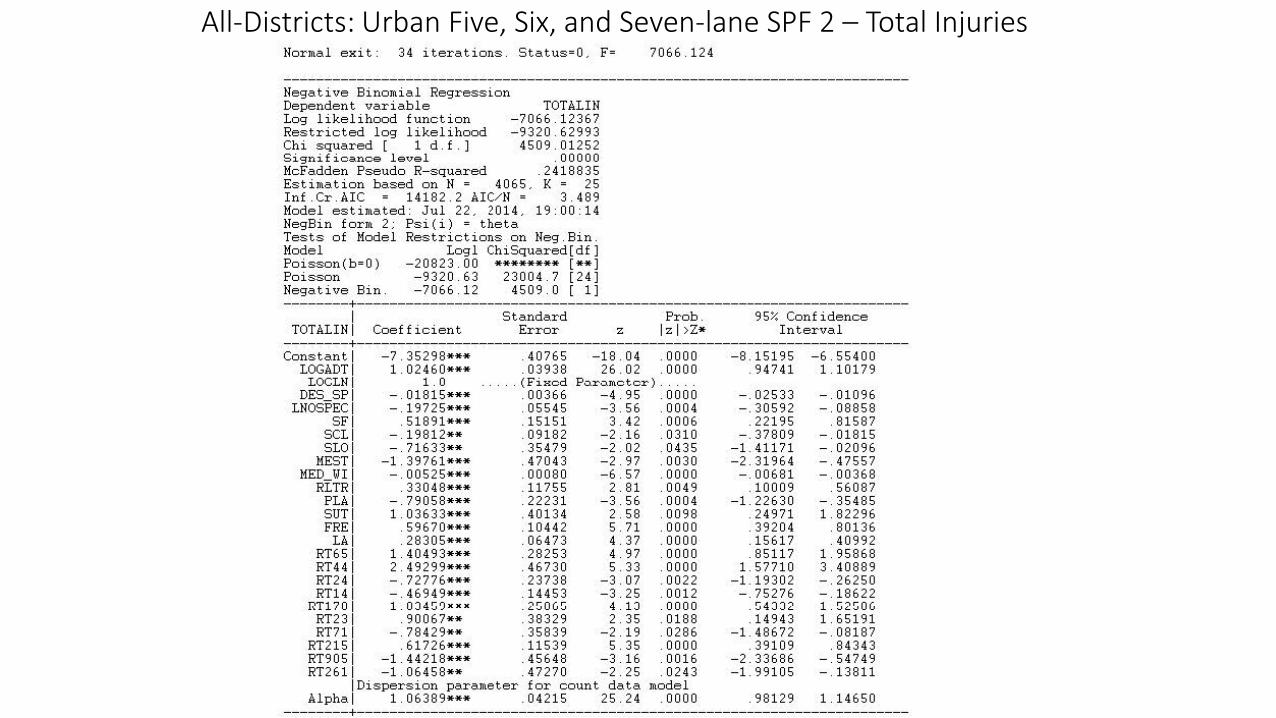
All-Districts: Urban Five, Six, and Seven-lane SPF 2 – Total Injuries Normal exit: 34 iterations. Status=O, F=


7066.124

--------+--------------------------------------------------------------------1 Standard Prob. 95% Con£ idence

TOTALINI Coefficient Error z lzi>Z* Interval --------+--------------------------------------------------------------------Constant -7.35298*** .40765 -18.04 .0000 -8.15195 -6.55400

LOGADT 1. 02460*** . 03938 26.02 . 0000 . 94741 1.10179 LOCLN 1. 0 ..... (Fixed Po.ro.motor).

DES SP -.01815*** .00366 -4.95 .0000 LNOSPEC -.19725*** .05545 -3.56 .0004

SF . 51891*** .15151 3. 42 . 0006 SCL -.19812** .09182 -2.16 .0310 SLO -.71633** .35479 -2.02 .0435

MEST -1.39761*** .47043 -2.97 .0030 MED WI -.00525*** .00080 -6.57 .0000

RLTR . 33048*** .11755 2. 81 . 0049 PLA -.79058*** .22231 -3.56 .0004 sur 1. 03633*** . 40134 2. sa . oo9a FRE . 596 70*** .10442 5. 71 . 0000

LA .28305*** .06473 4.37 .0000 RT65 1. 40493*** . 28253 4. 97 . 0000 RT44 2.49299*** .46730 5.33 .0000 RT24 -. 72776*** . 23738 -3. 07 . 0022 RT14 -.46949*** .14453 -3.25 .0012

RT170 1. OJ4G9x x x . 2GOGG 4 .13 . 0000 RT23 . 9006 7** . 38329 2. 35 . 0188 RT71 -. 78429** . 35839 -2.19 . 0286

RT215 . 61726*** .11539 5. 35 . 0000 RT905 -1. 44218*** . 45648 -3.16 . 0016 RT261 -1. 06458** . 4 7270 -2. 25 . 0243

Dispersion parameter for count data model

-.02533 -.30592

.22195 -.37809

-1.41171 -2.31964 -.00681

.10009 -1.22630

.24971

.39204

.15617

. 85117 1. 57710

-1.19302 -.75276

.G4JJ2

.14943 -1.48672

.39109 -2.33686 -1.99105

-.01096 -.08858

.81587 -.01815 -.02096 -.47557 -.00368

.56087 -.35485 1.82296

.80136

.40992 1.95868 3.40889 -.26250 -.18622 1.G2GOG 1.65191 -.08187

.84343 -.54749 -.13811

Alpha 1. 06389*** . 04215 25. 24 . 0000 . 98129 1.14650 --------+--------------------------------------------------------------------

All-Districts: Urban Eight Plus-lane SPF 1 – Total Noninjuries

All-Districts: Urban Eight Plus-lane SPF 1 – Total Fatalities

All-Districts: Urban Eight Plus-lane SPF 1 – Total Injuries

All-Districts: Urban Eight Plus-lane SPF 2 – Total Fatalities

Poisson Regression Dependent variable TOTALFA Log likelihood function -973.47059 Restricted log likelihood -1204.48431 Chi squared [ 10 d.f.] 462.02745 Significance level .00000 McFadden Pseudo R-squared .1917947 Estimation based on N = 5693. K = 11 Inf.Cr.AIC = 1968.9 AIC/N = .346 Model estimated: Jul 23. 2014. 18:34:05 Chi- squared= 6321.78433 RsqP= .1637 G -squared= 1425.10517 RsqD= .2448 Overdispersion tests: g=mu(i) 2.912 Overdispersion tests: g=mu(i)'2: 1.885 --------+--------------------------------------------------------------------

1 Standard Prob. 95% Confidence TOTALFAI Coefficient Error z lzi>Z* Interval

--------+--------------------------------------------------------------------Constant -11.9631*** 2.45858 -4.87 .0000 -16.7819 -7.1444

LOGADT . 86849*** .19794 4. 39 . 0000 . 48052 1. 25645 LOGLN 1. 0 ..... (Fixed Parameter).

RT99 1. 23512** . 51257 2. 41 . 0160 RT15 . 44218** . 20955 2.11 . 0348

RT710 . 75332** . 36457 2. 07 . 0388 RT405 -. 75905** . 33361 -2. 28 . 0229

RT22 2. 08494*** . 71480 2. 92 . 0035 RTlO . 51157*** .17753 2. 88 . 0040

SF 1. 00860** . 41879 2. 41 . 0160 RNOSPEC .28160** .13953 2.02 .0436

RT_IS_YI -.03618** .01750 -2.07 .0387

.23050

. 0314 7

. 03877 -1. 41291

.68395

.16362

.18779

.00813 -.07047

2.23973 .85289

1.46787 -.10518 3.48594

.85952 1.82942

.55506 -.00189


All-Districts: Urban Eight Plus-lane SPF 2 – Total NoninjuriesNormal exit: 38 iterations. Status=O, F=

Negative Binomial Regression Dependent variable TOTALNI Log likelihood function -12913.231&6 Restricted log likelihood -16854.05428 Chi squared [ 1 d.f.] 7881.64523 Significance level .00000 McFadden Pseudo R-squared .2338205 Estimation based on N = 5693. K 30 Inf.Cr.AIC 25886.5 AIC/N = 4.547 Model estimated: Jul 23. 2014. 03:29:30 NegBin form 2; Psi(i) = theta Tests of Model Restrictions on Neg.Bin. Model Log! ChiSquared[df] Poisson(b=O) -39988.00 ******** [**] Poisson -16854.05 46267.9 [29] Negative Bin. -12913.23 7881.6 [ 1]

12913.23

--------+-------------------------------------------------------------------1 Standard Prob. 95% Confidence

TOTALNII Coefficient Error z lzi>Z* Interval --------+-------------------------------------------------------------------Constant -11. 5163*** . 46426 -24.81 . 0000 -12.4262 -10.6063

LOGADT 1. 23988*** . 03821 32.45 . 0000 1.16499 1. 31478 LOGLN 1. 0 ..... (Fixed Parameter).

FRE . 62320** . 24588 2. 53 . 0113 RT210 -. 28744*** . 09244 -3.11 . 0019 RT280 -. 29829*** . 08153 -3. 66 . 0003

RT24 -. 47476*** .13301 -3.57 . 0004 RT29 2. 63456*** . 34479 7. 64 . 0000

LA . 08906*** . 03244 2. 75 . 0060 SF . 616 73*** .17131 3. 60 . 0003

SAC . 49017*** . 06389 7. 67 . 0000 RIV .19593*** .07096 2.76 .0058

MED WI -.00469*** .00067 -7.02 .0000 LAUXL .14673*** .04909 2.99 .0028 LTOLL .93852*** .28339 3.31 .0009

RMEDHOV -.16831*** .03577 -4.71 .0000 MEOTHER .54996*** .14128 3.89 .0001 MECABLG -.84813** .41269 -2.06 .0399 MEBRAIL -.44140*** .06611 -6.68 .0000

MEGRAILL -.33599** .16099 -2.09 .0369 MECONCR -.54357*** .19064 -2.85 .0044 MECONCB .20216*** .06400 3.16 .0016

RT14 . 56236*** .13155 4. 27 . 0000 SCL . 33092*** . 07030 4. 71 . 0000

SJ . 55938*** .15981 3. 50 . 0005 RT980 . 6 7325*** . 24337 2. 77 . 0057

.14128 -.46861 -.45808 -.73544 1.95878

.02548

.28096

.36494

.05685 -.00600

.05051

.38310 -.23842

.27305 -1.65698 -.57097 -.65151 -.91722

.07672

.30453

.19314

.24617

.19624

1.10512 -.10626 -.13850 -.21407 3.31034

.15265

.95249

.61539

.33501 -.00338

.24296 1.49395 -.09820

.82687 -.03927 -. 31183 -.02046 -.16993

.32759

.82018

. 46871

.87260 1.15025

All-Districts: Urban Eight Plus-lane SPF 2 – Total Noninjuries(contd)

RT680 I -. 33337*** .10234 -3. 26 . OOL RT22I . 92760~~ . 42236 2. 20 . 028:

RT110 I . 23600*** . 07323 3. 22 . 0013 RT215I . 40984*** .15636 2. 62 . 0088

!Dispersion parameter for count data model

-.53395 .09980 .09247 .10337

-.13279 1.75541

.37954

. 71631

Alpha I . 65274*** . 01866 34.98 . 0000 . 61617 . 68932 --------+--------------------------------------------------------------------Note: ***, **, * ==> Significance at 1%, 5%, 10% :evel. Fixed parameter is constrained to equal the va:ue or had a nonpositive st.error because of an earlier problem.

All-Districts: Urban Eight Plus-lane SPF 2 – Total Injuries Normal exit: 38 iterations. Status=O, F=


12956.00

--------+-----------------------------------------------------------------1 Standard Prob. 95% Confidence

TOTALINI Coefficient Error z lzi>Z* Interval --------+-----------------------------------------------------------------Constant -11. 4539*** . 46309 -24.73 . 0000 -12.3616 -10.5463

LOGADT 1. 23543*** . 03812 32. 41 . 0000 1.16072 1. 31013 LOGIN 1. 0 ..... (Fixed Parameter).

FRE . 61287** . 24464 2. 51 . 0122 RT210 -. 29061*** . 09188 -3 .16 . 0016 RT280 -. 30765*** . 08043 -3. 83 . 0001

RT24 -. 48381*** .13284 -3. 64 . 0003 RT29 2. 62033*** . 34318 7. 64 . 0000

LA .09176*** .03239 2.83 .0046 SF . 63691*** .16550 3. 85 . 0001

SAC . 48779*** . 06366 7. 66 . 0000 RIV .20670*** .07047 2.93 .0034

MED IJI -. 004 70*** . 0006 7 -7. 05 . 0000 LAUXL .14555*** . 04875 2. 99 . 0028 LTOLL . 92235*** . 28080 3. 28 . 0010

RMEDHOV -.17261*** .03564 -4.84 .0000 MEOTHER . 56139*** .13739 4. 09 . 0000 MECABLG -.83568** .39765 -2.10 .0356 MEBRAIL -. 42951*** . 06619 -6. 49 . 0000

MEGRAILL -.36115** .15447 -2.34 .0194 MECONCR -.54399*** .18914 -2.88 .0040 MECONCB . 20458*** . 06344 3. 22 . 0013

RT14 . 55250*** .13130 4. 21 . 0000 SCL . 33485*** . 06988 4. 79 . 0000

SJ . 56365*** .16049 3. 51 . 0004 RT980 . 66363*** . 24209 2. 74 . 0061

.13338 -.47069 -.46529 -.74417 1.94771

.02828

.31253

.36300

.06858 -.00601

.04999

.37200 -.24247

.29212 -1.61506 -.55925 -.66390 -. 91471

.08024

.29514

.19789

.24909

.18915

1.09236 -.11053 -.15001 -.22346 3.29294

.15523

.96129

.61257

.34482 -.00339

. 24110 1.47270 -.10275

.83067 -.05630 -.29978 -.05840 -.17327

.32892

.80985

.47180

.87821 1.13811

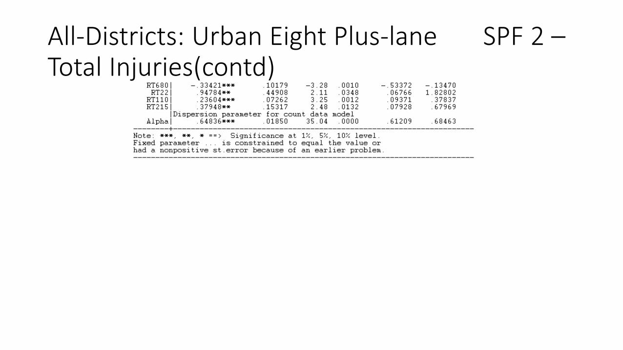
All-Districts: Urban Eight Plus-lane SPF 2 –Total Injuries(contd)

2. government association number 3. … · venky shankar and samer madanat 8. ... in the case of...

Documents