1.oluwaseyi ayodele ajibade, 2. optimisation...

A NNALS of Faculty Engineering Hunedoara – International Journal of Engineering Tome XVI [2018] | Fascicule 4 [November]

123 | F a s c i c u l e 4

1.Oluwaseyi Ayodele AJIBADE, 2.Johnson Olumuyiwa AGUNSOYE, 3.Sunday Ayoola OKE

OPTIMISATION OF WEAR PARAMETERS OF DUAL FILLER EPOXY COMPOSITES USING THE GREY RELATIONAL ANALYSIS 1,2.Department of Metallurgical and Materials Engineering, University of Lagos, Lagos, NIGERIA 3.Department of Mechanical Engineering, University of Lagos, Lagos, NIGERIA Abstract: Researchers have long examined wear of composites. More lately, material scientists and engineering scholars have explored cheap and low density solid waste by-products of manufacturing and process systems such as cenosphere fly-ash of coal’s combination in thermal power plants to enhance wear resistance of aluminum metal matrix composites in brake part applications. Hitherto, little is understood about the wear of agro-rooted fortified polymer composites. Furthermore, very less is known on wear optimization of agro-based polymer composites reinforced with pairs of blended particulates of any for orange peels, shells of coconut, periwinkle, palm kernel and egg. Building on two groups of scientific literature-composites and optimization- this research examined how dual blended polymer composites could be optimized using the grey relational analysis (GRA) in the presence of limited data for the composite development process. The GRA is illustrated as a configuration to achieve comprehension of the wear optimization procedure for the chosen composites. The offered procedure initiates a new research direction in dual mixed fortified polymer composites for the following reasons. First, a foremost attempt at optimizing any of the developed composites in a situation of limited data is reported. Second, the possible influence of variations of the orthogonal arrays on the wear outcome is a novelty documented for the wear outcome is a novelty documented for the first time in the polymer composite literature. The achieved outcome using the L16 orthogonal array revealed an optimal setting of A2B1C2D4 as the most advantageous grey run for all the composites. For the second goal of varying the orthogonal array, it was noted that the percentage differences obtained between the original and variant results that there could be improvement, stagnancy or decline in the obtained optimal results. The research offers a deep insight into the composite optimization procedure helpful in the development process, and is an extremely required bridge connecting the literature on composites and optimization. Keywords: wear, dual-filler composites, optimisation, grey relational analysis

1. INTRODUCTION Researchers across the composite fields such as natural, ceramics and metal matrices have long examined composite wear (Friedrich et al. 2002; Xuet al. 2004; Zhou et al., 2014; Tiwari and Bijwe, 2014; Bicer et al. 2015). More lately, material scientists and engineering scholars have explored cheap and low density solid wastes by-products of manufacturing and process systems. The early works in this respect are on industrial waste consisting of lime sludge (Kashyap and Datta, 2017), waste polyethylene terephthalate bottles coupled with marble dust (Cinar and Kar, 2018), industrial discarded fruit wastes (Binoj et al. 2018), fly ash cenosphere (Bora et al., 2018) saw dust, rise lust, fly ash and red mud (Prabu et al., 2017). A careful analysis of this stream of studies points out to two facts. First, there is an aggressive pursuit of outstanding properties of material being used. It means that cheapness, low density, high hardness, excellent impact properties and outstanding flexural characteristics are some of the notable concerns of the scholars in this area of research is the need for environmental complaint composites made up of natural reinforcements. Consequently, this paper concurs with the theories behind this stream of research to narrow the choices of fortifiers for the current investigation to solid wastes that will possibly meet up with the competitive properly benchmark and the environmental conscious fabrication to streamline choices of fortifiers to particulate orange peels, kernel shells, periwinkle shells, palm kernel shells and egg shells for the production of polymer composites for use in brake part applications. The direction of research elaborated in the current paper was embarked upon based on the fact that hitherto, little is understood about the wear of agro-rooted fortified polymer composites. Furthermore, very less is known on wear optimization of agro-rooted polymer composites reinforced with blended pairs of particulates of any of orange peels, shells of coconut, periwinkle, palm kernel and egg. It is very interesting to note that there are two literature fields that are apart till now. On one side several research efforts have been done in the composite literature where scholars are majority concerned with the characterization of composites: evaluation of hardness properties, impact behavior, tensile characteristics and the flexural properties of polymer composites. These were done when a new composite is developed, subjected to water absorption conditions and wear process. Efforts are made by scholars to enhance these properties with chemical treatments on the particulates also. This body of knowledge is a parallel with optimization literature of the most advantageous parametric values of systems. Now, converging these two literature (i.e. composites and optimization), this study has successfully produced a framework in which newly developed composites could be optimized using the grey relational analysis. In the following paragraphs, a brief review of literature in the domain of the current research is given.


124 | F a s c i c u l e 4

2. LITERATURE REVIEW Khan et al. (2013) used the chemical vapour deposition (CVD) procedure to produce carbon nano materials (CNMs) in two distinct structures namely carbon nano beads (Pi) and a combination of carbon nona tubes and carbon nano beads from unwanted polyethylene bags. Field emission scanning electron microscope (FESEM) was used to understand the morphology of the CNMs while the purity was studied with thermagravimetric analysis (TGA) and Ramanspectroscopy. The mechanical and tribological characteristics of the CNMs were contrasted with commercially available Multi Walled Carbon Nano Tubes (MWCNT) composites. They noticed that the in house produced CNMs exhibited superior mechanical and tribological behaviour over exhibited superior mechanical and tribological behaviour over the neat epoxy and commercial NWCNT composites. Sanchez-Sanchez et al. (2013) identified ultrasonic injection moulding as the most beneficial way for producing ultra-high molecular weight polyethylene (UHMWPE)/ graphite composites. The UHMWPE powder was mixed mechanically with the graphite at L5 and 7wt%. Further tensile samples were produced from uneven shaped pre-composite mixtures which were passed through ultrasonic injection moulding. In order to obtain the best working ultrasonic parameters and to harness the tensile strength of the composites, the Taguchi method was used; which showed that the mould temperature was the most important parameter. Although the inclusion of graphite resulted in a decrease in the crystallinity of all the samples, their thermal stability was found superior to the pure UHMDUPE. X-ray diffraction and scanning electronic micro copy showed the graphite was scrubbed off and scattered as a result of the ultrasonic processing. Fourier transform infrared spectra revealed that the molecular structure of the polymer matrix remained intact despite the inclusion of the graphite. Borba et al. (2018) noted that the friction riveting is a viable joining technology to the traditional mechanical fastening used for warm-reinforced polymer composite. In their work, they show cased the predictability of the direct-friction reverting for Ti 6Al 4V and carbon-fiber enriched polymer ether-ketone laminate single lap joints. α-Martensitic structures were deserved in the fixed rivet zone alongside the fiber and trapped polymer at the rivet composite interface. The mean ultimate lap shear force of 7.4±0.6 kN was obtained which bears correlation to the traditional lock-bolted angle lap joints. The obtained results showed that direct-friction riveting can be used as a viable substitute and can be enhanced for used in aircraft structures. Ridruguez-Tembleque and Aliabadi (2016) observed that computational modeling of fretting wear in fiber-reinforced composites is a complex job as a result of the interface and wear governing principles which encompasses micromechanical features like fiber orientation related to study direction or fiber volume fraction. In their investigation, they put forward a 3D Boundary Element Method composition to idealise the wear which was used to initiate fretting-wear in fiber-reinforced composites. They developed novel governing equations for friction and wear modeling for fiber reinforced composites and integrated into a make-shift langrian resolution scheme and used it to evaluate and investigate wear in a carbon FRP film. Chadda et al. (2017) appraised the fracture toughness and wear properties of dimethacrylate made for restorative visible-light cured composites enriched with hydroxyapatite (micro-filled) and silica/hydroxyapatite (micro-hybrid) compositions. They prepared two chains of composites were fabricated with reinforcements in the range of 20-50wt% while the fracture toughness (Ka) values were estimated using the single-edge-notch-beam (SENB) specimen in a 3-point bending test. It was observed that the composites with 20wt% fillers obtained the highest KQ value while the 50wt% filled composites exhibited the least value of KQ, regardless of the type of the filler used. The dry sliding test of the composites was performed on a pin-on-disk configuration using applied load, time, and sliding speed as parameters. It was discovered that the specific wear rates of the composites compared favourably for both micro-filled and micro-hybrid composites in terms of wear confrontation and fracture toughness. Higher wear confrontation was noticed in dental composites of 30-40 wt% fibre loadings. The morphology of the worn surface revealed deep scratches in the 50wt% filled composites. Garcia-Gonzalez et al. (2018) in their work, offer a new encompassing model for semi-crystalline polymers, mainly applied as matrices in different areas of applications. The encompassing model is created finite distortions inside a thermodynamically steady structure. Further, the model was executed using a finite element code and its parameters are mentioned for two biomedical polymers: Ultrahigh-molecular-weight polyethylene (VAMWPE) and high-density polyethylene. It was concluded that the model predicts the large spectrum of strain rate and temperatures, which gives room for optimization of novel composites which are effectively used as substitutes for joints prostheses. Chen et al. (2017) formulated a PUA-HA/PAA composite hydrogel by freezing-thawing, PEG dehydration and annealing methods. The optimal combination was selected with the aid of an orthogonal design method. It was observed that PVA and freezing-thawing cycles hide the highest influence on creep confrontation and stress relation rate of hydrogel, while the annealing temperature and freeze-thawing cycles have the highest


125 | F a s c i c u l e 4

influence on compressive elastic modules of hydrogel. The optimal characteristics combination was established as PVA-HA/PAA composite hydrogel with freezing-thawing cycles of 3, annealing temperature of 1200C, PVA 16%, HA 2%, PAA 4%. The PVA-HA/PAA composite hydrogel has a spongy arrangement framework which permits interfaces among PVA, HA and PAA in hydrogel which enriches the characteristics of the hydrogel. They also observed that the annealing treatment is beneficial to the crystalline and cross linking of hydrogel. It was therefore concluded that annealing the PVA-HA and PAA in hydrogel which enriches the characteristics of the hydrogel. They also observed that the annealing treatment is beneficial to the crystalline and cross linking of hydrogel. It was therefore concluded that annealing the PVA-HA/PAA hydrogel has good them ostability, strength and mechanical characteristics. Yuan et al. (2018) put forward a new production route to synthesize carbon nanotube (CNT) composite powders and apply them for selective laser sintering (SLS) process. It was found that at a minute enrichment of CNT (< 1wt%), the laser sintered composites demonstrated remarkable progress in electrical conductivity comparable to anti-static and conductive scope usable in aerospace and automobile applications. Worth of note, Yuan et al. (2018) observed that the thermal conductivity of laser sintered composites cannot compared favourably with of hot compressed. He et al. (2017) prepared a molecular model of polymer composites enriched with nano-SiO2 particles. They used the molecular dynamics simulations to investigate the improved tribological characteristics of the polymer/nano-sio2 composites experienced a reduction of 27 and 47.4%, respectively. He et al. (2017) also studied the interfacial relationship between polymer materials and nano-sio2 particles. Chetia et al. (2018) observed that natural fiber reinforced composites have attracted research interest as a result of their specific characteristics, non-carcinogenic and bio-degradability. Worthy of note among this class are bamboo and basalt which are cheap and offers superior mechanical behavior over unidirectional glass enriched plastic. In their work, they utilized the Taguchi by orthogonal array and grey relational analysis to establish optimal combination of factors to reduce delamination factor arising from drilling operations and maximize tensile strength. It was observed that the cutting speed and feed rate are the two delamination and tensile strength. The predicted results were verified comparably with the experimental results using confirmation experiments. Kumar and Panneerselvam (2016) established the mechanical and abrasive wear behavior of the Nylon 6 and GFR Nylon 6 composites. They used the injection molding machine to produce the Nylon 6 and GFR Nylon 6 composites for mechanical and wear test. The dry sliding wear test was performed a pin-on-disc set up a 320 grit applied load, sliding distance were studied at a temperature of 230C under humid conditions. It was observed that the specific wear rate was observed at 30wt% fiber loading. The analysis revealed that the abrasive weight less improved with higher load. Optimal and scanning electron microscopy were used to investigate the microstructure of the worn surfaces. Chang et al. (2014) analysed the two influence of filler reinforcement talc particles and glass fiber as secondary fillers in high ultra-high molecular weight polyethylene (UHMWPE) composites in their work. A pin-on-disc wear tester was used to study the wear and friction characteristics of these hybrid composites using applied load, sliding aped and sliding distances as parameters for the Box-Behnken design of response surface methodology (RSM). The RSM was used to optimize the explanatory variables to reduce the wear and friction. The analysis of variance (ANOVA) produced the regression models for the wear volume and average COF. It was observed that applied load, sliding speed and distance have remarkable influence on the wear and friction behavior of both VHMWPE composites. In order of importance, load, sliding distance and speed were found to be the most prominent. Aggarwal et al. (2017) harnessed both tensile strength (TS) and flexural strength (FS) of sisal-hemp fiber enriched high density polyethylene (HDPE) composite. In order to increase their linkage to the matrix, the fibers were treated with NaOH and maleic anyhydride. ANOVA regression modeling was used to model as the best fit. A mixture of 80% HDPE, 10% sisal and 10% heap produces maximum TS and FS of 20.3MPa and 15.5MPa, respectively. The TS and FS were founded to be more responsive to the fiber volume of sisal in the composite as shown in the Trace plot. Valasek et al. (2018) used practical experiments to illustrate the strength characteristics of white and brown coir fibres and biocomposites illustrated by vaccum infusion. The fibre surface was treated using NaOH solution treatment. It was observed that the interfacial adhesion was occasioned by a coarsening of the fibers as a result of chemical treatment strength of up to 58MPa and modulus of up to 1.87GPa. It was discovered that increase in the adhesion between fibre and epoxy resin happened as layers of lignin were removed from the fibers. The presence of the chemically treated fibres enhanced the matrix strength to 28.64MPa while the addition of white fibers to 20.22MPa. Suresh et al. (2018) carried out an investigation on erosion wear on PTFE/HNT nano composites using air jet erosion tester as per ASTM G76 standard. The response surface methodology (RSM) was used for the design of the experiments on the erosion tester. The parameters used are composition, pressure, with 3 levels while


126 | F a s c i c u l e 4

impingement angle was used at 4 levels for a fill factorial design of 36 experimental trials. Plots were used to depict the impingement angle and pressure on erosion wear are plotted. The plot shows that maximum wear bears correlation to low impingement angles and larger operating pressures. Xiao et al. (2014) produced a novel composite comprising nacre in an Al matrix through powder metallurgy and heat treatment routes. Mechanical properties were assessed using SEM, microhardness tester and profilometer. The hardness of the composites improved with higher loadings of nacre in the composite. The hardness of the 20wt% nacre improved by 40% over that of the Al. the best wear confrontation were found in the 1 and 5wt% nacre filling. The current work reveals that the mechanical behavior and control of wear process is achievable by optimizing the hybrid configuration. Saukarand Umamaheswarro (2017) noted that carbon fiber reinforced composites (CFRP) have found diverse usage as e result of its sufficient tensile strength, good specific modulus and unique physical properties. The CFRP drilling process produces serious challenges due to its layered make-up. Factor, the performance of drilling was investigated thrust force, surface roughness and delamination factor. The performance properties were more responsive to factors such as cutting, speed, depth of cut, feed and point angle. Nevertheless, the optimization of the process factors led to an efficient drilling. The optimization of the CFRP drilling process is targeted using the Ant Colony Algorithm (ACO) tool. In order to minimize the operating voltage and enhance device operation, a novel type of binary polymer composite dielectrics is formulated by introducing a minute amount of polyacrylic acid (PAA) into poly (oriethylmethacrylate) (PMMA). It was observed that malleable organic field-effect transistors (OFEFs) which makes use of PMMA: PAA dielectrics exhibits increased mobility and minimal threshold voltages with an operating voltage below 5V. it was also observed that the OFETS using the composite dielectric demonstrates improved operational steadiness during mechanical bending tests. With the use of disimilar radii. Sarkar et al. (2017) studied the tribological behavior of glass epoxy composite under different parameters. They used a pin-on-disc wear set-up and friction monitor to study experimentally the influence of normal loads and sliding velocities on the friction and wear properties of glass fiber enriched epoxy composite. The tests were carried out at normal loads of 5, 10, 20, 30, 40 and 50N and the sliding speeds of 0.5, 1, 2 and 0.3m/s. the time, normal load and sliding speed were found to have direct effect on friction and wear. It was found to have direct effect on friction and wear. It was observed that friction coefficient reduced with higher loadings and increases with rise in sliding speed for all sliding speeds and normal loads, respectively. A rise in normal loads and sliding speeds for all conditions increased the wear loss of the composite. Deepak et al. (2017) observed that the use of epoxy resin in many tribological was occasioned by heat, possibly besides friction. As a result, molybdenum was introduced at 5, 10 and 15wt% to enhance the wear properties of the composites. A control sample in this investigation was prepared without modification. The composite sample were investigated for their wear, tensile and flexural properties while the morphology of the worn surfaces was understand using scanning election microscopy. Punugupati et al. (2018) produced bonded silica ceramic composite with additions of boron nitride and silicon nitride with the use of gel casting, a near net-shape-production method. They formulated a mathematical model to establish the influence of load, sliding distance and sliding speed on the wear loss, while the response surface methodology using central composite face centered design with t6 points was used to investigate the influence of the parameters on wear. Karatas and Gokkaya (2018) carried out a literature investigation on machinability behavior and related issues for carbon fibre reinforced polymer (CFRP) and glass fibre reinforced polymer (GFRP) composites. The failure process was observed in the meaning of the CFRP and GFRP similar to those obtained for heterogenous materials and these results were obtained through the use of analysis of variance (ANOVA), artificial neural network (ANN) fuzzy interference system, harmony search (HS) algorithm, genetic algorithm (GA) Taguchi optimization, multi-criterion, optimization, analytical modeling, stress analysis, finite elements method, (FEM), data analysis and linear regression techniques. Optical and scanning electron microscopy and profilometry were used to understand procedure of failure and surface morphology. Patere and Lathkar (2018) concentrated on using polymer utilized on industry such as sugar roller bearing, pharmanceutical, milk processing and all food packaging outfits. In order to eradicate this challenge, this work concentrates on utilizing polymer matrix composites for bearing applications. They concentrated on optimizing the tribological factors of wear and friction of polymer composites with polytetrafloroethylene as the parent material enriched with 15, 20 and 25% glass fiber along 5% M0S2 which has lubrication and wear confrontation attributes. The unconventional TOPSIS optimization technique was used to optimize the tribological parameter. The Taguchi method was used in the design of the experiments while further analysis and examination was carried out with X-ray diffraction (XRD) analysis and scanning Electron microscopy (SEM).


127 | F a s c i c u l e 4

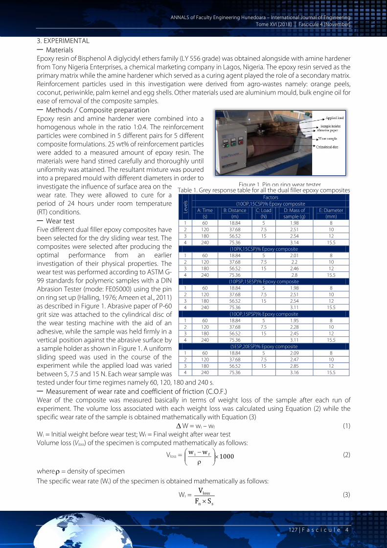
3. EXPERIMENTAL — Materials Epoxy resin of Bisphenol A diglycidyl ethers family (LY 556 grade) was obtained alongside with amine hardener from Tony Nigeria Enterprises, a chemical marketing company in Lagos, Nigeria. The epoxy resin served as the primary matrix while the amine hardener which served as a curing agent played the role of a secondary matrix. Reinforcement particles used in this investigation were derived from agro-wastes namely: orange peels, coconut, periwinkle, palm kernel and egg shells. Other materials used are aluminium mould, bulk engine oil for ease of removal of the composite samples. — Methods / Composite preparation Epoxy resin and amine hardener were combined into a homogenous whole in the ratio 1:0.4. The reinforcement particles were combined in 5 different pairs for 5 different composite formulations. 25 wt% of reinforcement particles were added to a measured amount of epoxy resin. The materials were hand stirred carefully and thoroughly until uniformity was attained. The resultant mixture was poured into a prepared mould with different diameters in order to investigate the influence of surface area on the wear rate. They were allowed to cure for a period of 24 hours under room temperature (RT) conditions. — Wear test Five different dual filler epoxy composites have been selected for the dry sliding wear test. The composites were selected after producing the optimal performance from an earlier investigation of their physical properties. The wear test was performed according to ASTM G-99 standards for polymeric samples with a DIN Abrasion Tester (mode: FE05000) using the pin on ring set up (Halling, 1976; Ameen et al., 2011) as described in Figure 1. Abrasive paper of P-60 grit size was attached to the cylindrical disc of the wear testing machine with the aid of an adhesive, while the sample was held firmly in a vertical position against the abrasive surface by a sample holder as shown in Figure 1. A uniform sliding speed was used in the course of the experiment while the applied load was varied between 5, 7.5 and 15 N. Each wear sample was tested under four time regimes namely 60, 120, 180 and 240 s. — Measurement of wear rate and coefficient of friction (C.O.F.) Wear of the composite was measured basically in terms of weight loss of the sample after each run of experiment. The volume loss associated with each weight loss was calculated using Equation (2) while the specific wear rate of the sample is obtained mathematically with Equation (3)

∆W = wi – wf (1) Wi = Initial weight before wear test; Wf = Final weight after wear test Volume loss (Vloss) of the specimen is computed mathematically as follows:

Vloss = 1000ww fi ×

ρ− (2)

whereρ= density of specimen The specific wear rate (Wr) of the specimen is obtained mathematically as follows:

Wr = sn

loss

SFV×

(3)

Figure 1. Pin on ring wear tester

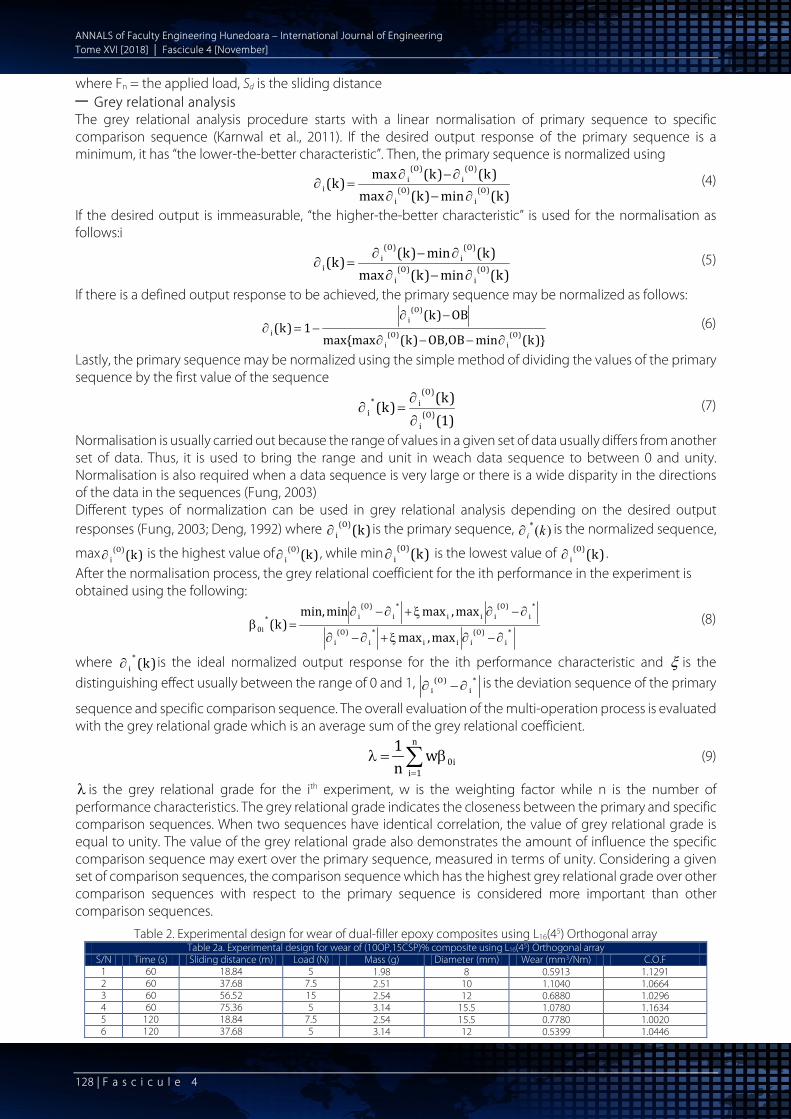
Table 1. Grey response table for all the dual filler epoxy composites Le

vels

Factors (10OP,15CSP)% Epoxy composite

A: Time (s)

B: Distance (m)

C: Load (N)

D: Mass of sample (g)

E: Diameter (mm)

1 60 18.84 5 1.98 8 2 120 37.68 7.5 2.51 10 3 180 56.52 15 2.54 12 4 240 75.36 3.14 15.5

(10PK,15CSP)% Epoxy composite 1 60 18.84 5 2.01 8 2 120 37.68 7.5 2.2 10 3 180 56.52 15 2.46 12 4 240 75.36 2.8 15.5

(10PSP,15ESP)% Epoxy composite 1 60 18.84 5 1.98 8 2 120 37.68 7.5 2.51 10 3 180 56.52 15 2.54 12 4 240 75.36 3.11 15.5

(10OP,15PSP)% Epoxy composite 1 60 18.84 5 1.95 8 2 120 37.68 7.5 2.28 10 3 180 56.52 15 2.45 12 4 240 75.36 3.11 15.5

(5ESP,20ESP)% Epoxy composite 1 60 18.84 5 2.09 8 2 120 37.68 7.5 2.47 10 3 180 56.52 15 2.85 12 4 240 75.36 3.16 15.5


128 | F a s c i c u l e 4

where Fn = the applied load, Sd is the sliding distance — Grey relational analysis The grey relational analysis procedure starts with a linear normalisation of primary sequence to specific comparison sequence (Karnwal et al., 2011). If the desired output response of the primary sequence is a minimum, it has “the lower-the-better characteristic”. Then, the primary sequence is normalized using

)k(min)k(max

)k()k(max)k( )O(

i)O(

i

)O(i

)O(i

i∂−∂

∂−∂=∂ (4)

If the desired output is immeasurable, “the higher-the-better characteristic” is used for the normalisation as follows:i

)k(min)k(max

)k(min)k()k( )O(i

)O(i

)O(i

)O(i

i∂−∂

∂−∂=∂ (5)

If there is a defined output response to be achieved, the primary sequence may be normalized as follows:

)}k(minOB,OB)k(max{max

OB)k(1)k( )O(

i)O(

i

)O(i

i∂−−∂

−∂−=∂ (6)

Lastly, the primary sequence may be normalized using the simple method of dividing the values of the primary sequence by the first value of the sequence

)1()k(

)k( )O(i

)O(i*

i∂

∂=∂ (7)

Normalisation is usually carried out because the range of values in a given set of data usually differs from another set of data. Thus, it is used to bring the range and unit in weach data sequence to between 0 and unity. Normalisation is also required when a data sequence is very large or there is a wide disparity in the directions of the data in the sequences (Fung, 2003) Different types of normalization can be used in grey relational analysis depending on the desired output responses (Fung, 2003; Deng, 1992) where )k()O(

i∂ is the primary sequence, )(* ki∂ is the normalized sequence,

max )k()O(i∂ is the highest value of )k()O(

i∂ , while min )k()O(i∂ is the lowest value of )k()O(

i∂ . After the normalisation process, the grey relational coefficient for the ith performance in the experiment is obtained using the following:

*i

)O(iii

*i

)O(i

*i

)O(iii

*i

)O(i*

i0max,max

max,maxminmin,)k(

∂−∂ξ+∂−∂

∂−∂ξ+∂−∂=β (8)

where )k(*i∂ is the ideal normalized output response for the ith performance characteristic and ξ is the

distinguishing effect usually between the range of 0 and 1, *i

)O(i ∂−∂ is the deviation sequence of the primary

sequence and specific comparison sequence. The overall evaluation of the multi-operation process is evaluated with the grey relational grade which is an average sum of the grey relational coefficient.

∑=

β=λn

1ii0w

n1

(9)

λ is the grey relational grade for the ith experiment, w is the weighting factor while n is the number of performance characteristics. The grey relational grade indicates the closeness between the primary and specific comparison sequences. When two sequences have identical correlation, the value of grey relational grade is equal to unity. The value of the grey relational grade also demonstrates the amount of influence the specific comparison sequence may exert over the primary sequence, measured in terms of unity. Considering a given set of comparison sequences, the comparison sequence which has the highest grey relational grade over other comparison sequences with respect to the primary sequence is considered more important than other comparison sequences.

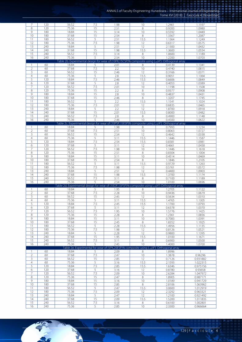
Table 2. Experimental design for wear of dual-filler epoxy composites using L16(45) Orthogonal array Table 2a. Experimental design for wear of (10OP,15CSP)% composite using L16(45) Orthogonal array

S/N Time (s) Sliding distance (m) Load (N) Mass (g) Diameter (mm) Wear (mm3/Nm) C.O.F 1 60 18.84 5 1.98 8 0.5913 1.1291 2 60 37.68 7.5 2.51 10 1.1040 1.0664 3 60 56.52 15 2.54 12 0.6880 1.0296 4 60 75.36 5 3.14 15.5 1.0780 1.1634 5 120 18.84 7.5 2.54 15.5 0.7780 1.0020 6 120 37.68 5 3.14 12 0.5399 1.0446


129 | F a s c i c u l e 4

7 120 56.52 7.5 1.98 10 1.2461 1.1597 8 120 75.36 15 2.51 8 0.9283 1.0980 9 180 18.84 15 3.14 10 0.5592 1.0449

10 180 37.68 15 2.54 8 1.3367 1.2087 11 180 56.52 5 2.51 15.5 1.1364 1.1249 12 180 75.36 7.5 1.98 12 0.6317 1.0575 13 240 18.84 5 2.51 12 2.1300 1.0432 14 240 37.68 15 1.98 15.5 1.3600 1.0554 15 240 56.52 7.5 3.14 8 1.0600 1.1189 16 240 75.36 5 2.54 10 1.2200 1.0703

Table 2b. Experimental design for wear of (10PK,15CSP)% composite using L16(45) Orthogonal array 1 60 18.84 5 2.01 8 0.4139 1.1341 2 60 37.68 7.5 2.2 10 0.4740 1.0815 3 60 56.52 15 2.46 12 0.3166 1.0371 4 60 75.36 5 2.8 15.5 0.9051 1.1364 5 120 18.84 7.5 2.46 15.5 0.6606 1.0849 6 120 37.68 5 2.8 12 0.4053 1.0389 7 120 56.52 7.5 2.01 10 1.1198 1.1508 8 120 75.36 15 2.2 8 0.9377 1.0908 9 180 18.84 15 2.8 10 0.4837 1.0431

10 180 37.68 15 2.46 8 1.3207 1.1745 11 180 56.52 5 2.2 15.5 1.1541 1.1024 12 180 75.36 7.5 2.01 12 0.6835 1.0465 13 240 18.84 5 2.2 12 1.8700 1.0918 14 240 37.68 15 2.01 15.5 0.8000 1.0482 15 240 56.52 7.5 2.8 8 0.4900 1.1148 16 240 75.36 5 2.46 10 0.4500 1.0622

Table 2c. Experimental design for wear of (10PSP,15ESP)% composite using L16(45) Orthogonal array 1 60 18.84 5 1.98 8 0.7993 1.1234 2 60 37.68 7.5 2.51 10 0.8063 1.0727 3 60 56.52 15 2.54 12 0.4642 1.0338 4 60 75.36 5 3.11 15.5 1.1446 1.1587 5 120 18.84 7.5 2.54 15.5 0.8381 1.0981 6 120 37.68 5 3.11 12 0.4661 1.0458 7 120 56.52 7.5 1.98 10 1.1446 1.1618 8 120 75.36 15 2.51 8 0.8304 1.1004 9 180 18.84 15 3.11 10 0.4514 1.0469

10 180 37.68 15 2.54 8 1.1846 1.2105 11 180 56.52 5 3.11 15.5 0.9729 1.1263 12 180 75.36 7.5 1.98 12 0.5761 1.0572 13 240 18.84 5 2.51 12 0.4400 1.0903 14 240 37.68 15 1.98 15.5 1.3700 1.1174 15 240 56.52 7.5 3.11 8 0.7100 1.1189 16 240 75.36 5 2.54 10 1.0100 1.0696

Table 2d. Experimental design for wear of (10OP,15PSP)% composite using L16(45) Orthogonal array 1 60 18.84 5 1.95 8 1.2705 1.1122 2 60 37.68 7.5 2.28 10 0.9436 1.0679 3 60 56.52 15 2.45 12 0.5634 1.0310 4 60 75.36 5 3.11 15.5 1.4765 1.1305 5 120 18.84 7.5 2.45 15.5 1.1700 1.0793 6 120 37.68 5 3.11 12 0.6378 1.0370 7 120 56.52 7.5 1.95 10 1.5776 1.1425 8 120 75.36 15 2.28 8 1.2361 1.0856 9 180 18.84 15 3.11 10 0.7083 1.0391

10 180 37.68 15 2.45 8 1.8352 1.1925 11 180 56.52 5 2.28 15.5 1.4956 1.1135 12 180 75.36 7.5 1.98 12 0.8126 1.0521 13 240 18.84 5 2.28 12 0.9800 1.1395 14 240 37.68 15 1.95 15.5 1.0100 1.1671 15 240 56.52 7.5 3.11 8 0.6900 1.0500 16 240 75.36 5 2.45 10 1.4000 1.0700

Table 2e. Experimental for wear of (5PK,20ESP)% composite using L16(45) Orthogonal array 1 60 18.84 5 2.09 8 1.8996 1 2 60 37.68 7.5 2.47 10 1.3878 0.96296 3 60 56.52 15 2.85 12 0.7126 0.931882 4 60 75.36 5 3.16 15.5 2.1593 1.022315 5 120 18.84 7.5 2.85 15.5 1.6346 0.975156 6 120 37.68 5 3.16 12 0.8780 0.93658 7 120 56.52 7.5 2.09 10 2.6284 1.047972 8 120 75.36 15 2.47 8 1.8905 0.987171 9 180 18.84 15 3.16 10 1.0189 0.941729

10 180 37.68 15 2.85 8 2.8106 1.063962 11 180 56.52 5 2.47 15.5 3.0600 1.012919 12 180 75.36 7.5 2.09 12 2.3292 0.963321 13 240 18.84 5 2.47 12 1.2100 0.921492 14 240 37.68 15 2.09 15.5 1.5200 1.011835 15 240 56.52 7.5 3.16 8 0.6100 1.002801 16 240 75.36 5 2.85 10 2.3300 0.966664


130 | F a s c i c u l e 4

Figure 2. Research scheme

4. RESULTS AND DISCUSSION — Optimal grey run The wear rates and corresponding C.O.F. for the wear of the five different dual filled composites are outlined in Table 2. Characteristic of a typical wear process, the lesser the wear rate, the higher the integrity of the material. Thus, “the lower-the-better” quality characteristic is the desired response used in this investigation. Consequently, the primary sequences of the wear rates and CO.F. for the composites were normalized using “the lower-the-better” methodology described in Equation (1). The lowest values of the wear rates and C.O.F. are set as primary sequences )k()O(

0∂ , k = 1-2, while the results of the sixteen

experiments are fixed as the specific comparison sequence )k()0(i∂

, i =1-16, k = 1-2. The normalized sequences were found to be the same for all the data sequences of the different composites as outlined in Table 2 and denoted as )k(*

0∂ and )k(*i∂ for the

primary and specific comparison sequences, respectively. The delta sequence is the difference is the between the primary and specific comparison sequence which is

defined as 01∆ = *i

)O(i ∂−∂ (10)

Table 3. Normalised data sequences for all the composites

Primary/Comparison sequence

Wear rate C.O.F

Primary sequence 1.0000 1.0000 Comparison sequence

Experiment 1 0.9676 0.385 Experiment 2 0.6452 0.6884 Experiment 3 0.9068 0.8664 Experiment 4 0.6615 0.2191 Experiment 5 0.8502 1 Experiment 6 1 0.7939 Experiment 7 0.5558 0.237 Experiment 8 0.7557 0.5355 Experiment 9 0.9878 0.7924

Experiment 10 0.4988 0 Experiment 11 0.6248 0.4054 Experiment 12 0.9422 0.7314 Experiment 13 0 0.8006 Experiment 14 0.4842 0.7416 Experiment 15 0.6729 0.4344 Experiment 16 0.5722 0.6695


131 | F a s c i c u l e 4

The same procedure was carried out for i =1-16 for all the composites where i =1-16 as described in Table 3. From the given data in Table 3, the maximum and minimum delta sequences were found to be the same for all the composites and were determined as follows:

0)2()1(1)2()1(

56min

1013max

=∆=∆=∆

=∆=∆=∆

The distinguishing effectξ is substituted into Equation (xxx) to calculate the grey relational coefficient. If the parameters are of equal importance, then ξ is taken as 0.5. The grey relational grade is obtained from the grey response table typical of the S/N ratio response table of the Taguchi method. Thus, the grey relational grade is calculated using the average of the factor levels described by the orthogonal array. In other words, the grey relational grade for factor level A1, is obtained by finding the average of the grey grades described by the arrangement in the orthogonal array. The same mathematical operation is used to obtain the grey response tables for all the composites.

Table 5. Grey response table for all the dual filler epoxy composites

Levels Factors

A: Time (s) B: Distance (m) C: Load (N) D: Mass of sample (g) E: Diameter (mm) 1 0.6621 0.7360* 0.6158 0.6264 0.5605 2 0.6991* 0.6116 0.6516* 0.5584 0.6187 3 0.6363 0.5824 0.6489 0.6719 0.7419* 4 0.5518 0.6193 0.6926* 0.6282

* means optimal grey grade An optimal grey setting of A2B1C2D4E3 was obtained as the optimal grey setting for the minimal wear rate and C.O.F. in all the dual filler epoxy composites. However, it is interpreted differently for all composites due to their individual sample masses. The (10OP,15CSP)% epoxy composite optimal setting can be translated as a time of 120 seconds, sliding distance of 18.84 m, applied load of 7.5 N, sample mass of 3.14 g and a diameter of 12 mm. For the (10PK,15CSP)% composite, the optimal grey setting can be read as time of 120 seconds, sliding distance of 18.84 m, applied load of 7.5 N, sample mass of 2.8 g and diameter of 12 mm. The optimal grey setting for the (10PSP,15ESP)% composite can be interpreted as time of 120 seconds, sliding distance of 18.84 m, applied load of 7.5 N, sample mass of 3.14 g as well as a diameter of 12 mm. The (10OP,15PSP)% optimal grey setting is described as time of 120 seconds, sliding distance of 18.84 m, applied load of 7.5 N, sample mass of 3.11 g and a diameter of 12 mm. Lastly, the optimal grey setting of the (5PK,20ESP)% composite is interpreted as time of 120 seconds, sliding distance of 18.84 m, load of 7.5 N, sample mass of 3.16 g and a diameter of 12 mm. — The most significant factor All the dual-filler filled epoxy composites were found to have the same optimal grey setting even though they have different wear rates and C.O.F. values. Thus, it is pertinent to understand what factor influences the different wear rate and C.O.F values in each of the composites. The grey relational analysis can be used to quantify the contributions of each parameter to the wear rate and CO.F as well as identify which parameter makes the highest contribution into the wear system of each composite. The wear rates and C.O.F for each of the composite’s 16 experimental trials are fixed as the primary sequences )k()O(

WR∂ and )k()O(COF∂ , k = 1-2, while

the factor level values in the sixteen experimental trials are designated as the specific comparison sequences, where )k()O(

A∂ , )k()O(B∂ , )k()O(

C∂ , )k)O(D∂ and )k()O(

E∂ , k = 1-2 for the five control factors. Normalisation was carried out simply by dividing each sequence by its first value as stated in Equation (7). The normalised sequences for each of the dual-filler epoxy composites are described by Table 3. The delta sequence was obtained by subtracting the normalised values from each of the primary sequences as described by Equation (10). The delta sequences and distinguishing effect were substituted into Equation (8) to calculate the grey relational coefficient. The averages obtained from each grey relational coefficient represent the grey relational grade for the different controllable factor. The grey relational grades, coefficient, primary and specific comparison sequences )k((*)

A∂ , )k((*)B∂ , )k((*)

C∂ , )k(*)D∂ and )k((*)

E∂ for each of the dual filler composites are shown in Table 8-12.

Table 4. Table of delta sequences

Delta sequence i0∆ (1) i0∆ (2)

Experiment 1 0.0324 0.615 Experiment 2 0.3548 0.3116 Experiment 3 0.0932 0.1336 Experiment 4 0.3385 0.7809 Experiment 5 0.1498 0 Experiment 6 0.0000 0.2061 Experiment 7 0.4442 0.763 Experiment 8 0.2443 0.4645 Experiment 9 0.0122 0.2076

Experiment 10 0.5012 1 Experiment 11 0.3752 0.5946 Experiment 12 0.0578 0.2686 Experiment 13 1.0000 0.1994 Experiment 14 0.5158 0.2584 Experiment 15 0.3271 0.5656 Experiment 16 0.4278 0.3305


132 | F a s c i c u l e 4

Table 6. Primary and specific comparison sequences for wear rate and C.O.F. results and experimental factor levels

Experimental trial

Specific comparison sequences

A: (Time, s)

B: (Distance, m)

C: (Load, N)

D: (Mass of sample, g) E:

(Diameter, m) (10OP,15CSP)%

(10PK,15CSP)%

(10PSP,15ESP)%

(10OP,15PSP)%

(5PK,20ESP)%

1 60 18.84 5 1.98 2.01 1.98 1.95 2.09 8 2 60 37.68 7.5 2.51 2.2 2.51 2.28 2.47 10 3 60 56.52 15 2.54 2.46 2.54 2.45 2.85 12 4 60 75.36 5 3.14 2.8 3.14 3.11 3.16 15.5 5 120 18.84 7.5 2.54 2.46 2.54 2.45 2.85 15.5 6 120 37.68 5 3.14 2.8 3.14 3.11 3.16 12 7 120 56.52 7.5 1.98 2.01 1.98 1.95 2.09 10 8 120 75.36 15 2.51 2.2 2.51 2.28 2.47 8 9 180 18.84 15 3.14 2.8 3.14 3.11 3.16 10

10 180 37.68 15 2.54 2.46 2.54 2.45 2.85 8 11 180 56.52 5 2.51 2.2 2.51 2.28 2.47 15.5 12 180 75.36 7.5 1.98 2.01 1.98 1.98 2.09 12 13 240 18.84 5 2.51 2.2 2.51 2.28 2.47 12 14 240 37.68 15 1.98 2.01 1.98 1.95 2.09 15.5 15 240 56.52 7.5 3.14 2.8 3.14 3.11 3.16 8 16 240 75.36 5 2.54 2.46 2.54 2.45 2.85 10

Experimental trial

Primary sequences (10OP,15CSP)% (10PK,15CSP)% (10PSP,15ESP)% (10OP,15PSP)% (5PK,20ESP)%

Wear rate C.O.F Wear rate C.O.F Wear rate C.O.F Wear rate C.O.F Wear rate C.O.F 1 0.5913 1.1291 0.4139 1.1341 0.7993 1.1234 1.2705 1.1122 1.8996 1.1069 2 1.1040 1.0664 0.4740 1.0815 0.8063 1.0727 0.9436 1.0679 1.3878 1.0659 3 0.6880 1.0296 0.3166 1.0371 0.4642 1.0338 0.5634 1.0310 0.7126 1.0315 4 1.0780 1.1634 0.9051 1.1364 1.1446 1.1587 1.4765 1.1305 2.1593 1.1316 5 0.7780 1.0020 0.6606 1.0849 0.8381 1.0981 1.1700 1.0793 1.6346 1.0794 6 0.5399 1.0446 0.4053 1.0389 0.4661 1.0458 0.6378 1.0370 0.8780 1.0367 7 1.2461 1.1597 1.1198 1.1508 1.1446 1.1618 1.5776 1.1425 2.6284 1.1600 8 0.9283 1.0980 0.9377 1.0908 0.8304 1.1004 1.2361 1.0856 1.8905 1.0927 9 0.5592 1.0449 0.4837 1.0431 0.4514 1.0469 0.7083 1.0391 1.0189 1.0424

10 1.3367 1.2087 1.3207 1.1745 1.1846 1.2105 1.8352 1.1925 2.8106 1.1777 11 1.1364 1.1249 1.1541 1.1024 0.9729 1.1263 1.4956 1.1135 3.0600 1.1212 12 0.6317 1.0575 0.6835 1.0465 0.5761 1.0572 0.8126 1.0521 2.3292 1.0663 13 2.1300 1.0432 1.8700 1.0918 0.4400 1.0903 0.9800 1.1395 1.2100 1.0200 14 1.3600 1.0554 0.8000 1.0482 1.3700 1.1174 1.0100 1.1671 1.5200 1.1200 15 1.0600 1.1189 0.4900 1.1148 0.7100 1.1189 0.6900 1.1122 0.6100 1.1100 16 1.2200 1.0703 0.4500 1.0622 1.0100 1.0696 1.4000 1.0679 2.3300 1.0700

Table 7. Primary and specific comparison sequences after normalisation

Experimental trial Specific comparison sequences Primary sequences

(10OP,15CSP)% Epoxy composite Wear rate C.O.F.

A B C D E 1 1 1 1 1 1.0 1 1 2 1 2 1.5 1.267677 1.25 1.867073 0.944469 3 1 3 3 1.282828 1.5 1.163538 0.911877 4 1 4 1 1.585859 1.9375 1.823102 1.030378 5 2 1 1.5 1.282828 1.9375 1.315745 0.887432 6 2 2 1 1.585859 1.5 0.913073 0.925162 7 2 3 1.5 1 1.25 2.10739 1.027101 8 2 4 3 1.267677 1.0 1.569931 0.972456 9 3 1 3 1.585859 1.25 0.945713 0.925427

10 3 2 3 1.282828 1.0 2.260612 1.070499 11 3 3 1 1.267677 1.9375 1.921867 0.99628 12 3 4 1.5 1 1.5 1.068324 0.936587 13 4 1 1 1.267677 1.5 3.602232 0.923922 14 4 2 3 1 1.9375 2.300017 0.934727 15 4 3 1.5 1.585859 1.0 1.79266 0.990966 16 4 4 1 1.282828 1.25 2.06325 0.947923

(10PK,15CSP)% Epoxy composite 1 1 1 1 1 1.0 1 1 2 1 2 1.5 1.0945 1.25 1.1452 0.95362 3 1 3 3 1.2238 1.5 0.7649 0.91447 4 1 4 1 1.393 1.9375 2.1867 1.002028 5 2 1 1.5 1.2238 1.9375 1.5960 0.9566 6 2 2 1 1.393 1.5 0.9792 0.9160 7 2 3 1.5 1 1.25 2.7054 1.0147 8 2 4 3 1.0945 1.0 2.2655 0.9618 9 3 1 3 1.393 1.25 1.1686 0.9197


133 | F a s c i c u l e 4

10 3 2 3 1.2238 1.0 3.1908 1.0356 11 3 3 1 1.0945 1.9375 2.7883 0.9720 12 3 4 1.5 1 1.5 1.6513 0.9227 13 4 1 1 1.0945 1.5 4.518 0.9627 14 4 2 3 1 1.9375 1.9328 0.9242 15 4 3 1.5 1.393 1.0 1.1838 0.9829 16 4 4 1 1.2238 1.25 1.0872 0.9366

(10PSP,15PSP)% Epoxy composite 1 1 1 1 1 1.0 1 1 2 1 2 1.5 1.2676 1.25 1.0087 0.9548 3 1 3 3 1.2828 1.5 0.5807 0.9202 4 1 4 1 1.5707 1.9375 1.432 1.0314 5 2 1 1.5 1.2828 1.9375 1.0485 0.9774 6 2 2 1 1.5707 1.5 0.5831 0.9309 7 2 3 1.5 1 1.25 1.432 1.0341 8 2 4 3 1.2676 1.0 1.0389 0.9795 9 3 1 3 1.5707 1.25 0.5647 0.9319

10 3 2 3 1.2828 1.0 1.482047 1.0775 11 3 3 1 1.5707 1.9375 1.2171 1.0025 12 3 4 1.5 1 1.5 0.7207 0.941 13 4 1 1 1.2676 1.5 0.5504 0.9705 14 4 2 3 1 1.9375 1.714 0.9946 15 4 3 1.5 1.5707 1.0 0.8882 0.9959 16 4 4 1 1.2828 1.25 1.2636 0.9521

(10OP,15PSP)% Epoxy composite 1 1 1 1 1 1.0 1 1 2 1 2 1.5 1.1692 1.25 0.7427 0.9601 3 1 3 3 1.2564 1.5 0.4434 0.9269 4 1 4 1 1.5948 1.9375 1.1621 1.0164 5 2 1 1.5 1.2564 1.9375 0.9208 0.9704 6 2 2 1 1.5948 1.5 0.502 0.9323 7 2 3 1.5 1 1.25 1.2417 1.0272 8 2 4 3 1.1692 1.0 0.9729 0.976 9 3 1 3 1.5948 1.25 0.5574 0.9342

10 3 2 3 1.25641 1.0 1.4444 1.0721 11 3 3 1 1.1692 1.9375 1.1771 1.0011 12 3 4 1.5 1.0153 1.5 0.6395 0.9459 13 4 1 1 1.1692 1.5 0.7713 1.0245 14 4 2 3 1 1.9375 0.7949 1.0493 15 4 3 1.5 1.5948 1.0 0.543 0.944 16 4 4 1 1.2564 1.25 1.1019 0.962

(5ESP,15PKSP)% Epoxy composite 1 1 1 1 1 1.0 1 1 2 1 2 1.5 1.1818 1.25 0.7305 0.9629 3 1 3 3 1.3636 1.5 0.3751 0.9318 4 1 4 1 1.5119 1.9375 1.1367 1.0223 5 2 1 1.5 1.3636 1.9375 0.8604 0.9751 6 2 2 1 1.5119 1.5 1.0367 1 7 2 3 1.5 1 1.25 1.1600 0.96296 8 2 4 3 1.1818 1.0 1.0927 0.931882 9 3 1 3 1.5119 1.25 1.0424 1.022315

10 3 2 3 1.3636 1.0 1.1777 0.975156 11 3 3 1 1.1818 1.9375 1.1212 1 12 3 4 1.5 1 1.5 1.0663 0.96296 13 4 1 1 1.1818 1.5 1.0200 0.931882 14 4 2 3 1 1.9375 1.1200 1.022315 15 4 3 1.5 1.5119 1.0 1.1100 0.975156 16 4 4 1 1.3636 1.25 1.0700 1

Table 8. The grey relational coefficient and grey relational grades of the (10OP,15CSP)% composites

Wear rate Grey relational coefficient A (Time) B (Distance) C (Load) D (Mass) E (Diameter)

1 1 1 1 1 1 2 0.56 0.9168 0.7799 0.6607 0.5739 3 0.8713 0.4438 0.4146 0.9073 0.7575 4 0.5728 0.4024 0.6125 0.8311 0.9019 5 0.6173 0.8227 0.8759 0.9725 0.6283 6 0.5038 0.5742 0.9373 0.6343 0.6416 7 0.9113 0.6215 0.6817 0.5131 0.5507 8 0.7196 0.3762 0.4764 0.7943 0.6484 9 0.3494 0.9643 0.3877 0.6458 0.7755

10 0.5988 0.849 0.6376 0.5441 0.4546


134 | F a s c i c u l e 4

11 0.5058 0.5762 0.5853 0.6408 0.9853 12 0.3636 0.3333 0.7509 0.9447 0.7089 13 0.7351 0.36 0.3333 0.3333 0.3333 14 0.3936 0.8301 0.6502 0.473 0.7435 15 0.3333 0.5483 0.8164 0.8494 0.5701 16 0.363 0.4308 0.5503 0.5993 0.5638

Grey relational grade 0.5874 0.6281 0.6556 0.7089* 0.6773 C.O.F.

1 1 1 1 1 1 2 0.9651 0.592 0.6527 0.5054 0.6321 3 0.9458 0.4231 0.3333 0.471 0.4716 4 0.9806 0.3402 0.9717 0.3729 0.3666 5 0.5802 0.9315 0.6302 0.4552 0.3333 6 0.5886 0.5876 0.9331 0.3333 0.4773 7 0.6125 0.437 0.6883 0.9241 0.702 8 0.5994 0.3359 0.3399 0.528 0.9502 9 0.4257 0.9536 0.3399 0.3334 0.618

10 0.4435 0.6223 0.3511 0.6087 0.8817 11 0.4342 0.4332 0.9964 0.549 0.358 12 0.427 0.3333 0.6495 0.8389 0.4823 13 0.3333 0.9527 0.9321 0.49 0.4768 14 0.3341 0.5898 0.3357 0.8351 0.3436 15 0.3382 0.4325 0.6722 0.357 0.9831 16 0.335 0.3341 0.9525 0.4965 0.6348

Grey relational grade 0.5839 0.5811 0.6736* 0.5686 0.6069

Table 9. The grey relational coefficients and grey relational grades for (10PK,15CSP)% composite

Wear rate Grey

relational coefficient

A (Time)

B (Distance)

C (Load)

D (Mass)

E (Diameter)

1 1 1 1 1 1 2 0.9093 0.6301 0.7594 0.9712 0.9351 3 0.861 0.3945 0.3333 0.9739 0.6724 4 0.551 0.4454 0.4849 0.6832 0.8582 5 0.7828 0.7096 0.9208 0.8214 0.8154 6 0.8579 0.5879 0.9818 0.8053 0.7434 7 0.6736 0.8317 0.481 0.5009 0.509 8 0.8458 0.4564 0.6034 0.5938 0.5436 9 0.4429 0.8962 0.3789 0.884 0.9488

10 0.8841 0.5501 0.8541 0.4653 0.4078 11 0.8731 0.8731 0.3845 0.5026 0.6394 12 0.5192 0.3827 0.8807 0.7243 0.9088 13 0.7376 0.2927 0.241 0.3333 0.3333 14 0.4133 0.9559 0.5115 0.6472 0.9969 15 0.3408 0.445 0.7795 0.8911 0.8914 16 0.3334 0.3334 0.9276 0.926 0.9026

Grey relational

grade 0.6891 0.6115 0.6576 0.7327 0.7566*

C.O.F. 1 1 1 1 1 1 2 0.9707 0.5952 0.6562 0.6286 0.6309 3 0.9473 0.4245 0.3333 0.4352 0.4638 4 0.9987 0.3391 0.998 0.3788 0.3513 5 0.5958 0.9318 0.6574 0.4716 0.3406 6 0.5865 0.5866 0.9255 0.3333 0.4645 7 0.6095 0.4366 0.6824 0.9419 0.6829 8 0.597 0.3361 0.3384 0.6425 0.93 9 0.425 0.9504 0.3339 0.3351 0.6054

10 0.4391 0.9233 0.3467 0.5589 0.9343 11 0.4312 0.4314 0.9739 0.6608 0.3441 12 0.4254 0.3333 0.6436 0.7554 0.4674 13 0.3361 0.9529 0.9655 0.644 0.4853 14 0.3333 0.5909 0.3343 0.759 0.3333 15 0.3376 0.4327 0.6685 0.3677 0.9675 16 0.3342 0.3343 0.9427 0.4536 0.6178

Grey relational

grade 0.5854 0.5999 0.675* 0.5854 0.6011

Table 10. The grey relational coefficients and grey relational grades for (10PSP,15ESP)% composite

Wear rate Grey


A (Time)

B (Distance)

C (Load)

D (Mass)

E (Diameter)

1 1 1 1 1 1 2 0.9949 0.6232 0.7125 0.6601 0.7232 3 0.8044 0.4039 0.3348 0.4174 0.4067 4 0.7996 0.3896 0.7381 0.7838 0.5549 5 0.6444 0.8385 0.7295 0.6823 0.4148 6 0.549 0.5364 0.7449 0.3374 0.4074 7 0.9414 0.5111 0.9471 0.5379 0.4237 8 0.6421 0.3563 0.383 0.6874 0.5251 9 0.4146 0.7902 0.3333 0.3333 0.4791

10 0.5318 0.8628 0.4451 0.7163 0.3333 11 0.4917 0.479 0.8486 0.5872 0.4666 12 0.4307 0.3333 0.6097 0.643 0.4471 13 0.3333 0.3865 0.7303 0.4122 0.3989 14 0.43 0.8453 0.4863 0.4133 0.7382 15 0.3566 0.437 0.6656 0.4243 0.8494 16 0.3866 0.3746 0.822 0.9632 0.9788

Grey relational

grade 0.6094 0.5729 0.6581* 0.5999 0.5717

C.O.F. 1 1 1 1 1 1 2 0.9708 0.594 0.656 0.6474 0.6192 3 0.9496 0.4237 0.3333 0.5882 0.4529 4 0.9795 0.34 0.9706 0.4439 0.3463 5 0.595 0.9314 0.6655 0.6574 0.3333 6 0.5843 0.5886 0.9377 0.3896 0.4575 7 0.6087 0.4375 0.6906 1.4851 0.6898 8 0.5955 0.3361 0.3397 0.6815 0.9592 9 0.4208 0.9574 0.3345 0.39 0.6015

10 0.4387 0.6219 0.351 0.8276 0.8609 11 0.4293 0.4336 0.9976 0.4268 0.3392 12 0.4219 0.3333 0.6504 1.3318 0.462 13 0.3315 0.9526 0.9725 0.6686 0.4755 14 0.3333 0.5894 0.3414 1.7143 0.3373 15 0.3334 0.4328 0.6735 0.4231 0.9917 16 0.3302 0.3341 0.956 0.6247 0.6171

Grey relational

grade 0.5826 0.5816 0.6793 0.7687* 0.5964


135 | F a s c i c u l e 4

Table 11. The grey relational coefficients and grey relational grades for (10OP,15PSP)% composite

Wear rate Grey


A (Time)

B (Distance)

C (Load)

D (Mass)

E (Diameter)

1 1 1 1 1 1 2 0.8704 0.5719 0.6279 0.5616 0.5101 3 0.7564 0.3965 0.3333 0.4019 0.3333 4 0.9142 0.3718 0.8874 0.558 0.4052 5 0.6156 0.955 0.6882 0.6195 0.3419 6 0.5357 0.5286 0.7196 0.3333 0.3461 7 0.9415 0.4886 0.8319 0.6933 0.9847 8 0.6272 0.3569 0.3867 0.7357 0.9513 9 0.4144 0.7915 0.3435 0.345 0.4327

10 0.5263 0.7515 0.451 0.744 0.5431 11 0.4867 0.4796 0.8783 0.9857 0.4099 12 0.4227 0.3333 0.5976 0.593 0.3804 13 0.3486 0.8802 0.8482 0.5787 0.4203 14 0.3503 0.5823 0.3669 0.7271 0.3161 15 0.3333 0.4061 0.5718 0.3419 0.3161 16 0.3736 0.367 0.9261 0.7796 0.7811

Grey relational

grade 0.5948 0.5788 0.6536* 0.6248 0.5295

C.O.F. 1 1 1 1 1 1 2 0.9649 0.5949 0.651 0.6131 0.6252 3 0.9454 0.4241 0.3333 0.5013 0.4576 4 0.9893 0.3385 0.9715 0.3641 0.3442 5 0.5974 0.9313 0.6618 0.5367 0.3333 6 0.5886 0.5885 0.9387 0.3333 0.46 7 0.6109 0.4363 0.6867 0.9243 0.6846 8 0.5987 0.3355 0.3386 0.6317 0.9529 9 0.4251 0.9587 0.3341 0.334 0.605

10 0.4421 0.6216 0.3496 0.6426 0.8729 11 0.4332 0.433 0.9964 0.6634 0.3405 12 0.4265 0.3333 0.6516 0.8267 0.466 13 0.3392 0.9525 0.9316 0.6961 0.5042 14 0.3411 0.589 0.3469 0.8704 0.3525 15 0.3333 0.4261 0.6706 0.3373 0.8963 16 0.3346 0.3345 0.9522 0.5295 0.6268

Grey relational

grade 0.5856 0.5811 0.6759* 0.6127 0.5951

Table 12. The grey relational coefficients and grey relational grades for (5ESP,20ESP)% composite

Wear rate Grey


A (Time)

B (Distance)

C (Load)

D (Mass)

E (Diameter)

1 1 1 1 1 1 2 0.8722 0.542 0.6304 0.5688 0.5226 3 0.7464 0.364 0.3333 0.3759 0.3357 4 0.9308 0.3441 0.9056 0.6134 0.4152 5 0.6174 0.915 0.6723 0.5429 0.3455 6 0.5446 0.4941 0.7093 0.3619 0.354 7 0.9448 0.4817 0.9185 0.6081 0.8097 8 0.6467 0.3333 0.3956 0.7613 0.9918 9 0.4274 0.7641 0.3475 0.379 0.4434

10 0.5474 0.7427 0.4632 0.837 0.5425 11 0.5697 0.5195 0.6824 0.5812 0.6351 12 0.509 0.3513 0.8273 0.7247 0.6749 13 0.3535 0.8054 0.7833 0.5221 0.3971 14 0.365 0.5559 0.3736 0.7487 0.3333 15 0.3333 0.3593 0.5268 0.3333 0.4558 16 0.3987 0.3513 0.8528 0.8129 0.9604

Grey relational

grade 0.6129 0.5577 0.6513* 0.6107 0.576

C.O.F. 1 1 1 1 1 1 2 0.9765 0.5941 0.6581 0.568 0.6263 3 0.9576 0.4233 0.3333 0.3999 0.4585 4 0.9857 0.3377 0.9788 0.3701 0.4585 5 0.6003 0.9839 0.6633 0.4255 0.3333 6 0.5914 0.5881 0.9422 0.3333 0.4606 7 0.6178 0.4375 0.6966 0.8572 0.7043 8 0.6031 0.335 0.3393 0.5965 0.974 9 0.4278 0.963 0.3344 0.3352 0.6095

10 0.4429 0.6186 0.3481 0.4898 0.8827 11 0.4365 0.4331 0.9876 0.6302 0.3423 12 0.4304 0.3333 0.6583 0.8871 0.4727 13 0.3333 0.9508 0.9294 0.5249 0.454 14 0.3399 0.6057 0.3421 0.9606 0.342 15 0.3393 0.4319 0.6753 0.361 0.9942 16 0.3366 0.3335 0.9688 0.4202 0.6294

Grey relational

grade 0.5886 0.5855 0.6784* 0.5724 0.6088

The calculated grey relational grades for each of the composites described in Tables 8-12, can be grouped into matrix form as follows: Thus for the (10OP,15CSP)% composite, we have:

αααααααααα

=αE)(C.O.F,D)(C.O.F,C)(C.O.F,B)(C.O.F,A)(C.O.F,

E)(Wr,D)(Wr,C)(Wr,B)(Wr,A)Wr,(

=

6069.05686.06736.05811.05839.06773.07089.06556.06281.05874.0

Breaking down the matrix, we have ( )E)(Wr,D)(Wr,C)(Wr,B)(Wr,A),Wr,(1Row ααααα=

= ( )6773.0,7089.0,6556.0,6281.0,5874.0 ( )E)(C.O.F,D)(C.O.F,C)(C.O.F,B)(C.O.F,A),C.O.F,(2Row ααααα= = ( )6069.0,5686.0,6739.0,5811.0,5839.0

( ) ( )5839.05874.0A(C.O.F,A),(Wr,1 Col =αα= ( ) ( )5811.06281.0B(C.O.F,B),(Wr,2 Col =αα= ( ) ( )6736.06556.0C(C.O.F,C),(Wr,3 Col =αα=

( ) ( )5686.07089.0D(C.O.F,D),(Wr,4 Col =αα= ( ) ( )6069.06773.0E(C.O.F,E),(Wr,5 Col =αα=

The grey relational grade matrix for the (10OP,15CSP)% composite displays the values of the grey relational grade for the controllable factors to the wear rate and C.O.F. of the composite, respectively. The first direction it


136 | F a s c i c u l e 4

can be used is to identify the output response of the wear process that is more influenced by the controllable factors. As a result, the level of influence each controllable factor exhibits over the output responses of the wear process can be determined. The output response most influenced is determined by selecting the maximum of the rows i.e. max (Row 1, Row 2) = Row 1 = (0.5874, 0.6281, 0.6556, 0.7089, 0.6773). This means the primary sequence of wear rate )k()o(

Wr∂ is the stronger of the primary sequences for the (10OP,15CSP)% composite. In other words, the output response of wear rate bears a stronger correlation to the controllable factors in the dry sliding wear process of the composite than the C.O.F. Practically, the wear rate was more affected by the controllable wear parameters than the C.O.F. The values of the grey relational grades of the controllable factor A, B, C, D and E to both the wear behaviour responses of wear rate and C.O.F are described in Columns 1, 2, 3, 4 and 5, respectively. Thus, the second direction of using the grey relational grade matrix is that the specific influence each controllable factor contributes to the output responses could be determined. The factor making the most significant contribution is the maximum of the columns i.e. max Columns 1, 2, 3, 4 and 5. Thus, we have max (Col 1, Col 2, Col 3, Col 4, Col 5) = ( ) ( )6736.06556.0C(C.O.F,C),(Wr,3 Col =αα= . From Tables eee and vvv, it can be seen that the applied load exhibits the highest comparability sequences among the wear parameters. This indicates that the applied load bears the highest correlation to the wear behaviour output responses of wear rate and C.O.F. Therefore, the applied load was the most significant factor to the wear of the (10OP,15CSP)% epoxy composite. The degree of importance each controllable factor exhibits can also be determined by Rows 1 and 2 of the grey matrix. It has been observed that the wear rate was observed to be the stronger of the primary sequences. Going through Row 1, the order of importance each controllable factor exerts over the wear rate can be determined. This gives the order of importance as follows: D)Wr,(α >

E)Wr,(α > C)Wr,(α > B)Wr,(α > A)Wr,(α . In order words, the order of importance is mass of sample, diameter, load, distance and time. For Row 2, we have C)Wr,(α > E)Wr,(α > A)Wr,(α > B)Wr,(α >

D)Wr,(α . This translates to applied load, diameter, time, distance and mass of sample. The order of importance for the controllable factors changed considerably due to the differences in the output response being considered. This indicates that the controllable factors plays different roles and in different degrees in influencing the wear rates and C.O.F. of the (10OP,15CSP)% composite. The same operation was carried out using the grey grades of the remaining four composites to the grey grade matrix as follows: For the (10PK,15CSP)% epoxy composite, we have:

=

E)(C.O.F,D)(C.O.F,C)(C.O.F,B)(C.O.F,A)(C.O.F,E)(Wr,D)(Wr,C)(Wr,B)(Wr,A)Wr,(

6011.05854.0675.05999.05854.07566.07327.06576.06115.06891.0

For the (10PSP,15ESP)% epoxy composite, we have:

γγγγγγγγγγ

=γE)(C.O.F,D)(C.O.F,C)(C.O.F,B)(C.O.F,A)(C.O.F,


5964.07687.06793.05816.05826.05717.05999.06581.05729.06094.0

For the (10OP,15PSP)% epoxy composite, we have:

κκκκκκκκκκ

=κE)(C.O.F,D)(C.O.F,C)(C.O.F,B)(C.O.F,A)(C.O.F,


5921.06127.06759.05811.05856.05295.06248.06536.05788.05948.0

For the (5ESP,20ESP)% epoxy composite, we have:

ηηηηηηηηηη

=ηE)(C.O.F,D)(C.O.F,C)(C.O.F,B)(C.O.F,A)(C.O.F,


6088.05724.06784.05855.05886.0576.06107.06513.05577.06129.0

The summary of the more influenced row and most influential columns, order of importance of the factors in the output responses from the grey grade matrices and their practical implications are presented in Table 13.


137 | F a s c i c u l e 4

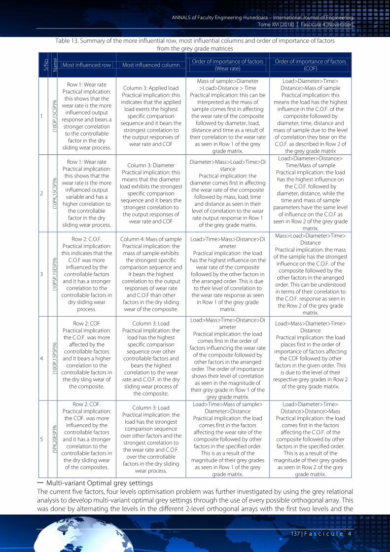
Table 13. Summary of the more influential row, most influential columns and order of importance of factors from the grey grade matrices

S/N

o

Nam

e

Most influenced row Most influenced column Order of importance of factors

(Wear rate) Order of importance of factors

(COF)

1

(10O

P,15

CSP)

%

Row 1: Wear rate Practical implication: this shows that the

wear rate is the more influenced output

response and bears a stronger correlation to the controllable

factor in the dry sliding wear process.

Column 3: Applied load Practical implication: this indicates that the applied

load exerts the highest specific comparison

sequence and it bears the strongest correlation to the output responses of

wear rate and COF

Mass of sample>Diameter >Load>Distance > Time

Practical implication: this can be interpreted as the mass of

sample comes first in affecting the wear rate of the composite

followed by diameter, load, distance and time as a result of

their correlation to the wear rate as seen in Row 1 of the grey

grade matrix.

Load>Diameter>Time> Distance>Mass of sample Practical implication: this

means the load has the highest influence in the C.O.F. of the

composite followed by diameter, time, distance and

mass of sample due to the level of correlation they bear on the C.O.F. as described in Row 2 of

the grey grade matrix

2

(10P

K,15

CSP)

%

Row 1: Wear rate Practical implication: this shows that the

wear rate is the more influenced output variable and has a

higher correlation to the controllable factor in the dry

sliding wear process.

Column 3: Diameter Practical implication: this means that the diameter

load exhibits the strongest specific comparison

sequence and it bears the strongest correlation to the output responses of

wear rate and COF

Diameter>Mass>Load>Time>Distance

Practical implication: the diameter comes first in affecting the wear rate of the composite

followed by mass, load, time and distance as seen in their

level of correlation to the wear rate output response in Row 1

of the grey grade matrix.

Load>Diameter>Distance> Time/Mass of sample

Practical implication: the load has the highest influence on

the C.O.F. followed by diameter, distance, while the

time and mass of sample parameters have the same level

of influence on the C.O.F as seen in Row 2 of the grey grade

matrix.

3

(10P

SP,1

5ESP

)%

Row 2: C.O.F. Practical implication: this indicates that the

C.O.F was more influenced by the

controllable factors and it has a stronger

correlation to the controllable factors in

dry sliding wear process.

Column 4: Mass of sample Practical implication: the mass of sample exhibits

the strongest specific comparison sequence and

it bears the highest correlation to the output

responses of wear rate and C.O.F than other

factors in the dry sliding wear of the composite.

Load>Time>Mass>Distance>Diameter

Practical implication: the load has the highest influence on the

wear rate of the composite followed by the other factors in the arranged order. This is due to their level of correlation to

the wear rate response as seen in Row 1 of the grey grade

matrix.

Mass>Load>Diameter>Time> Distance

Practical implication: the mass of the sample has the strongest

influence on the C.O.F. of the composite followed by the

other factors in the arranged order. This can be understood in terms of their correlation to the C.O.F. response as seen in the Row 2 of the grey grade

matrix.

4

(10O

P,15

PSP)

%

Row 2: COF Practical implication: the C.O.F. was more

affected by the controllable factors

and it bears a higher correlation to the

controllable factors in the dry sling wear of

the composite.

Column 3: Load Practical implication: the

load has the highest specific comparison sequence over other

controllable factors and bears the highest

correlation to the wear rate and C.O.F. in the dry sliding wear process of

the composite.

Load>Mass>Time>Distance>Diameter

Practical implication: the load comes first in the order of

factors influencing the wear rate of the composite followed by other factors in the arranged

order. The order of importance shows their level of correlation

as seen in the magnitude of their grey grade in Row 1 of the

grey grade matrix.

Load>Mass>Diameter>Time> Distance

Practical implication: the load places first in the order of

importance of factors affecting the COF followed by other

factors in the given order. This is due to the level of their

respective grey grades in Row 2 of the grey grade matrix.

5

(5PK

,20E

SP)%

Row 2: COF. Practical implication: the COF. was more influenced by the

controllable factors and it has a stronger

correlation to the controllable factors in the dry sliding wear of the composites.

Column 3: Load Practical implication: the

load has the strongest comparison sequence

over other factors and the strongest correlation to the wear rate and C.O.F.

over the controllable factors in the dry sliding

wear process.

Load>Time>Mass of sample> Diameter>Distance

Practical implication: the load comes first in the factors

affecting the wear rate of the composite followed by other factors in the specified order.

This is as a result of the magnitude of their grey grades

as seen in Row 1 of the grey grade matrix.

Load>Diameter>Time> Distance>Distance>Mass

Practical implication: the load comes first in the factors affecting the C.O.F. of the

composite followed by other factors in the specified order.

This is as a result of the magnitude of their grey grades

as seen in Row 2 of the grey grade matrix.

— Multi-variant Optimal grey settings The current five factors, four levels optimisation problem was further investigated by using the grey relational analysis to develop multi-variant optimal grey settings through the use of every possible orthogonal array. This was done by alternating the levels in the different 2-level orthogonal arrays with the first two levels and the


138 | F a s c i c u l e 4

remaining two levels in order to solve the present problem. As a result, robust set of results were obtained from the optimal grey settings by varying the levels appropriately. The results obtained by varying the levels in different orthogonal arrays are summarized in Table 14.

Table 14. Summary of results using different orthogonal arrays and alternate levels

S/N Orthogonal array Optimal grey

setting Variant of levels

used Interpretation

1 L825 A2B1C2D1E1

Using normal levels 1 and 2

Time of 120 seconds, distance of 18.84 m, load of 7.5 N, mass of 1.98 g and diameter of 8 mm.

Using variant levels 1 and 3

Time of 120 seconds, distance of 18.84 m, load of 15 N, mass of 1.98 g and diameter of 8 mm.




Time of 240 seconds, distance of 37.68 m, load of 15 N, sample mass of 2.51 g and diameter of 10 mm.





2 L1225

A1B1C2D2E2


Time of 60 seconds, distance of 18.84 m, load of 7.5 N, sample mass of 2.51 g and diameter of 10 mm.




Time of 60 seconds, distance of 18.84 m, load of 15 N, sample mass of 3.14 g and diameter of 15.5 mm.

A1B1C2D2E2





2 L1225 A1B1C2D2E2 Using variant levels 3 and 4


3 L1625 A1B1C1D1E2


Time of 60 seconds, distance of 18.84 m, load of 5 N, sample mass of 1.98 g and diameter of 10 m.


Time of 60 seconds, distance of 18.84 m, load of 5 N, sample mass of 1.98 g and diameter of 12 m.


Time of 60 seconds, distance of 18.84 m, load of 5 N, sample mass of 1.98 g and diameter of 15.5 m.


Time of 120 seconds, distance of 37.68 m, load of 7.5 N, mass of 2.51 g, diameter of 12 mm.


Time of 120 seconds, distance of 37.68 m, load of 7.5 N, mass of 2.51 g and diameter of 15.5 mm.


Time of 180 seconds, distance of 56.52 m, load of 7.5 N, mass of 2.54 g and diameter of 15.5 mm.

4 L2735 A1B1C1D2E3 Using normal levels 1, 2 and 3

Time of seconds, distance of 18.84 m, load of 5 N, sample mass of 2.51 g and diameter of 12 mm.

5 L3225 A1B1C2D1E1




Time of 60 seconds, distance of 18.84 m, load of 15 N, mass of 1.98 g, diameter of 8 mm.


Time of 60 seconds, distane of 18.84 m, load of 15 N, mass of 1.98 g and diameter of 8 mm.



5 L3225 A1B1C2D1E1





For each of the orthogonal array used, the results from the orthogonal array using the first two levels was designated as primary, while the results obtained using the variant levels are termed the specific comparison results. The percentage difference of the two results can be obtained as follows:

% difference = (specific comparison array results – primary orthogonal array results)×100 (primary orthogonal array results)

=

−

−

−

−

−

P

PSC

P

PSC

P

PSC

P

PSC

P

PSC

EEE

,D

DD,

CCC

,B

BB,

AAA

where, ASC results are from using levels 1 and 3, AP results are from levels 1 and 2 =

×

−×

−×

−×

−×

−100

EEE

,100D

DD,100

CCC

,100B

BB,100

AAA

P

PSC

P

PSC

P

PSC

P

PSC

P

PSC

% difference = ( ) ( ) ( ) ( ) ( )[ ]0,0,100,0,0 The same operation was carried for all the orthogonal array and the results are summarized in Table 15 as follows.


139 | F a s c i c u l e 4

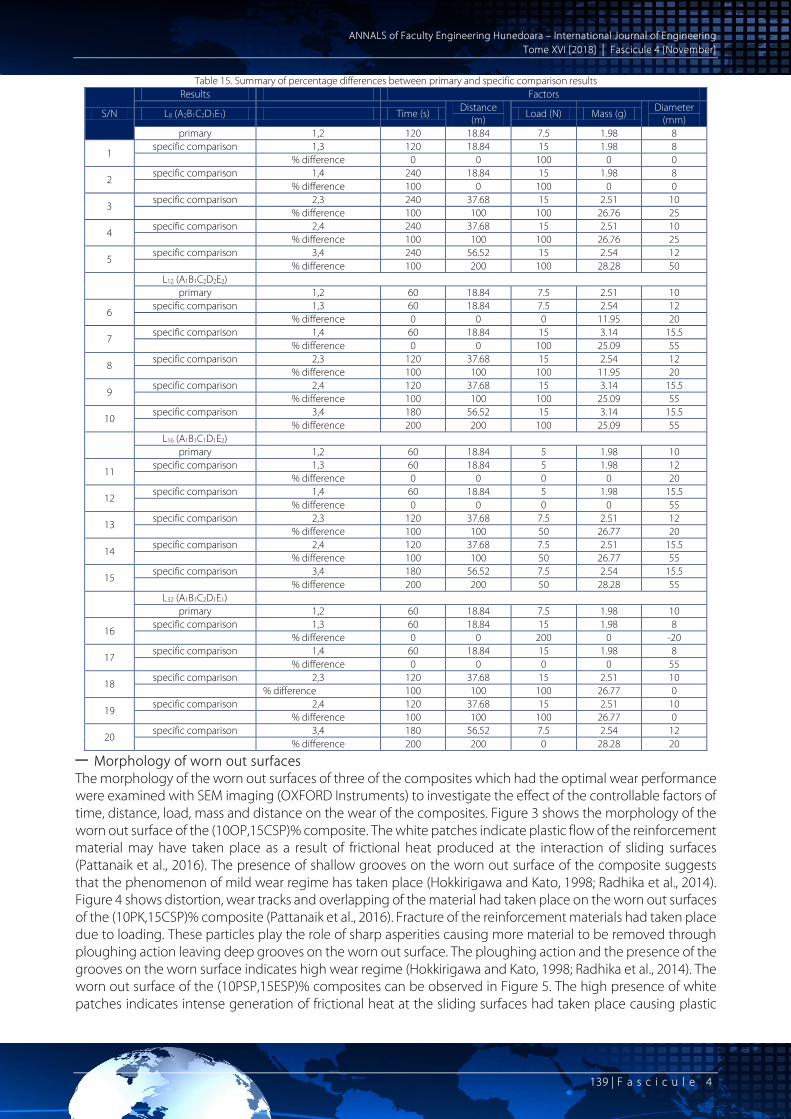
Table 15. Summary of percentage differences between primary and specific comparison results

S/N

Results Factors

L8 (A2B1C2D1E1) Time (s) Distance (m)

Load (N) Mass (g) Diameter (mm)

primary 1,2 120 18.84 7.5 1.98 8

1 specific comparison 1,3 120 18.84 15 1.98 8

% difference 0 0 100 0 0


% difference 100 0 100 0 0


% difference 100 100 100 26.76 25


% difference 100 100 100 26.76 25


% difference 100 200 100 28.28 50

L12 (A1B1C2D2E2)

primary 1,2 60 18.84 7.5 2.51 10

6 specific comparison 1,3 60 18.84 7.5 2.54 12

% difference 0 0 0 11.95 20

7 specific comparison 1,4 60 18.84 15 3.14 15.5

% difference 0 0 100 25.09 55


% difference 100 100 100 11.95 20


% difference 100 100 100 25.09 55


% difference 200 200 100 25.09 55

L16 (A1B1C1D1E2)

primary 1,2 60 18.84 5 1.98 10






% difference 100 100 50 26.77 20

14 specific comparison 2,4 120 37.68 7.5 2.51 15.5

% difference 100 100 50 26.77 55

15 specific comparison 3,4 180 56.52 7.5 2.54 15.5

% difference 200 200 50 28.28 55

L32 (A1B1C2D1E1)

primary 1,2 60 18.84 7.5 1.98 10


% difference 0 0 200 0 -20




% difference 100 100 100 26.77 0


% difference 100 100 100 26.77 0


% difference 200 200 0 28.28 20

— Morphology of worn out surfaces The morphology of the worn out surfaces of three of the composites which had the optimal wear performance were examined with SEM imaging (OXFORD Instruments) to investigate the effect of the controllable factors of time, distance, load, mass and distance on the wear of the composites. Figure 3 shows the morphology of the worn out surface of the (10OP,15CSP)% composite. The white patches indicate plastic flow of the reinforcement material may have taken place as a result of frictional heat produced at the interaction of sliding surfaces (Pattanaik et al., 2016). The presence of shallow grooves on the worn out surface of the composite suggests that the phenomenon of mild wear regime has taken place (Hokkirigawa and Kato, 1998; Radhika et al., 2014). Figure 4 shows distortion, wear tracks and overlapping of the material had taken place on the worn out surfaces of the (10PK,15CSP)% composite (Pattanaik et al., 2016). Fracture of the reinforcement materials had taken place due to loading. These particles play the role of sharp asperities causing more material to be removed through ploughing action leaving deep grooves on the worn out surface. The ploughing action and the presence of the grooves on the worn surface indicates high wear regime (Hokkirigawa and Kato, 1998; Radhika et al., 2014). The worn out surface of the (10PSP,15ESP)% composites can be observed in Figure 5. The high presence of white patches indicates intense generation of frictional heat at the sliding surfaces had taken place causing plastic


140 | F a s c i c u l e 4

flow and overlapping of the reinforcement particles in the matrix of the composite. The absence of cracks and grooves on the surface of the composite means the phenomenon of mild wear regime on the worn out surface.

Figure 3. SEM micrographs of worn surface of

(10OP,15CSP)% Epoxy composite

Figure 4. (10PK,15CSP)% composite Composite wear refers to the removal of materials from the surface of composites, commonly called erosion, but such a process could be minimized through the optimization process, entailing the choice of the most advantageous parametric values in the wear process. In this research, the tool referred to as the grey relational analysis is built on to develop a framework with which the composites wear process for a newly fabricated composite class could be minimized in a situation of limited data for experimentation. This novel framework of creating a unique optimization offers some new understanding, which are discussed as follows. First, at present, for the natural reinforced composites and the five chosen reinforcements for composites specially, single reinforcements are used for the polymer composites. In evaluating the wear performance of this single reinforced composite, a measured quantity is obtained, which could be at best being enhanced through particles treatments. The volumetric ratio of the reinforcement in the composite via combination with the matrix is due by trial and error. In this situation, having two little or two high volumetric ratios of fortifiers in combination with the matrix could be deficient or excessive (wasteful) in the tribological property desired. In this paper, it is asserted that the introduction of an additional fortifier for wear enhancement in paired mixture of fortifiers in composite can build up an elevated wear performance. This framework strengthens the composite community’s understanding of the impact of a second fortifier in radically enhancing the wear accomplishment of the new composite. Although the research is not conducted to consider more than two pairs of national particulates at time, nevertheless, the framework presented in this work lays the foundation for future studies to exploit the outcomes of the effects of combining at least three fortifiers incorporated in a matrix for the most outstanding wear performance. Second, studies on wear of polymeric composites have principally directed attention to the evaluation on the wear process in terms of the parametric values of the coefficient of friction as well as the wear of the polymeric composite. While the knowledge added by this body of studies provide essential foundation to pursue research in this domain. It is argued in this research that the values previously obtained in earlier studies may be sub-optimal and fabrication decisions made on these values may be in error. To correct this anormaly, in the present research, the notion of optimization that limited data may be available from the wear evaluation process. In particular, this research employs the grey relational analysis to develop a framework in which the most advantageous parametric quantities for the wear process of the newly developed composite could be appraised. It is argued that despite limited in the available data, and inspite of the uncertain nature of the process, the grey relational analysis can offer a necessary foundation for researchers to engage in research that shifts from sub-optimal value appraisal for the dual blended fortified composites. This permits a novel launch of research into an area where optimization appears to be an alien in research. Beyond the direction of the attention to the arguments made in this research, other viewpoints are possible, which could shed more light on the highlighted path of research. For instance, the metal matrix composite

Figure 5. (10PSP,15ESP)% composite


141 | F a s c i c u l e 4

literature has advanced to the incorporation of fillers beyond fortifiers, this making the elements outside the matrix to be at least three. Further studies could concur to this, using three elements (substances) as fortifiers and evaluating the optimization of this combination with the grey relational analysis. Second, beyond the grey relational analysis, the availability of outstanding optimization tools are abundant in the optimization literature. The whale algorithm, the Taguchi method, the Taguchi-ABC and Taguchi-Parento are also new variants of the Taguchi model that could be explored. 5. CONCLUSIONS A systematic optimisation of the dry sliding parameters of the dual output responses of wear rate and C.O.F of five different dual filler particles filled epoxy composites has been carried out in this work using the grey relational analysis. The investigation into the optimisation process of the wear parameters of the composites using the grey relational analysis has helped to understand the interplay of different factors in the output responses of the wear process. The correlation of the controllable factors to the output responses was understood in terms of the magnitude of the grey grade of each controllable factor. It also represents the level of correlation and its order of importance for each specific output response. The work showed that different operations can be performed with the grey relational analysis such as the optimal grey run and most significant factor by using different normalisation methods. Also, different optimal settings were derived through the use of variant levels. A number of useful findings deduced from this investigation are highlighted as follows: Optimal grey setting: An optimal grey setting of A2B1C2D4E3 was established as the optimal setting of the parameters for the five

different composites. This is because the dry sliding wear process was performed under the same conditions for the composites.

However, the optimal grey setting of the composites can be read differently due to the individual mass of sample component in each of the composite (factor level D4).

The most significant factor: The grey relational was used to determine the more influenced output response and the most influential

factor from the data sequences for each of the composite using a grey grade matrix. This work also established the order of importance of the controllable factors as they influenced the output

responses of wear rate and C.O.F. separately. Multi-variant Optimal grey settings: This work showed that 2-level based orthogonal arrays can be used in a 4-level based optimisation problem

by alternating the conventional factor levels with variant factor levels. Multi-variant optimal grey settings were obtained which produced wide variety of results that can be

applied to different wear regimes. The percentage differences obtained between the original and variant results shows that there could be

improvement, non-improvement or decline in the existing optimal results. References [1] Halling J., 1976. Introduction to Tribology, University of Salford, pp. 42-46. [2] Ameen H.A., Hassan K.S. and Mubarak E.M.M., 2011. Effect of loads, sliding speeds and times on the wear rate for

different materials, American Journal of Scientific and Industrial Research, Vol. 2, No. 1, pp. 99-106. [3] Deng J.L., 1992. The essential methods of Grey systems, Huazhong University of Science and Technology, Press,

Wuhan. [4] Zhou S., Zhang Q., Huang J., Ding D., 2014, Friction and wear behaviours of polyamide-based composite blended

with polyphenylene sulfide, Journal of Thermoplastic Composite Materials, Vol. 27, No.7, pp. 977-99 [5] Tiwari S, and Bijwe J, 2014, Influence of fiber-matrix interface on abrasive wear performance of polymer composites,

Journal of Reinforced Plastic and Composites, Vol. 33, No.2, pp. 115-126. [6] Xu H.H.K., Quinn J.B., Giuseppetti, 2004, Wear and mechanical properties of nano-silica-fused whisker composites,

Research Reports (Biomaterials and bioengineering), Vol. 83, No. 12, pp. 930-935 [7] Bicer AZY, Karakis D., Dogan A., Mert F., 2015, A comparison of wear rate of direct and indirect resin composites: A two

body wear abrasion test, Journal of Composite Materials, Vol.49, No. 21 pp. 2599-2607 [8] Friedrich k, Reinicke R and Zhang Z., 2002, Wear of Polymer composites, Proceedings of Institution of Mechanical

Engineers: Part J-Engineering Tribology, Vol. 216, pp.415-426 [9] Kashyap S., Datta D., 2017, Reusing industrial line sludge waste as a filler in polymeric composites Materials Today:

Proceedings, Vol.4, pp. 2946-2955. [10] CinarME and Kar F., 2018 Characterization of composite produced from waste PET and marble dust, Construction and

Building Materials, Vol. 163, pp. 734-741. [11] Binoj J.S., Raj R.E., Indran S., 2018, Characterisation of industrial discarded fruit waste (Tamarindus India L.) as potential

attentive for man-made vitreous fiber in polymer composites, Process Safety and Environmental Protection, Vol. 116, pp.527-2018

[12] Bora P.J., Porwal J., Vinoyk.J., Kishore, Ramamurthy P.C., Madras G., 2018, Industrial waste fly ash cenosphere composites based broad band microwave absorber, Composites Part B, Vol. 134, pp. 151-163.


142 | F a s c i c u l e 4

[13] Prabu V.A., Johnson RDT, Amuthakkannan P., ManikandanV., 2017, Usage of industrial wastes as particulate composite for environmental management: Hardness, tensile and impact studies, Journal of Environmental Chemical Engineering, Vol.5, pp. 1289-1301.

[14] Valasek P., D’Amato R., Muller M. and Ruggiero A., 2018. Mechanical properties and abrasive wear of white/brown coir epoxy composites, Composites Part B, Vol. 146, pp. 88-97.

[15] Xiao H., Shin Y., Li P., Sue H.J. and Liang H., 2014. A new composite designed to resist wear, Materials and Design, Vol. 36, pp. 749-756.

[16] Suresh G., Vasu V. and Raghavendra G., 2018. Optimization of Input Parameters on Erosion Wear Rate of PTFE/HNT filled nano composites, Materials Today: Proceedings, Vol. 5, pp. 1462-1469.

[17] Aggarwal L., Sinha S., Bhatti M.S. and Gopta V.K., 2017. Mixer design optimization with fractured surface to paragraphy of mechanical properties of polymer biocomposites, Journal of the Taiwan Institute of Chemical Engineers, Vol. 74, pp. 272-280.

[18] Sankar N.R. and Umamaheswarro P., 2017. Multi objective optimization of CFRP Composite Drilling Using Ant Colony Algorithm, Materials Today: Proceddings, Vol. 5, pp.4855-4860.

[19] Sarkar P., Modak N. and Sahoo P., 2017. Effect of normal load and velocity on continuous sliding friction and wear Behaviour of Woven Glass Fiber Reinforced Epoxy Composite, Materials Today: Proceedings, Vol. 4, pp 3082-3092.

[20] Liu Z., Yin Z., Chen S-C., Dai S., Huang J. and Zhang Q., 2018. Binary polymer composite dielectrics for flexible low voltage organic field-effect transistors, Organic Electronics, Vol.53, pp. 205-212.

[21] Patare P.M. and Lathkar G.S., 2018. Optimization of Glass Fiber and MOS2 filled PTFE Composites Using Non Traditional Optimisation Techniques, Materials Today: Proceedings, Vol. 5, pp. 7310-7319.

[22] Karatas M.A. and Gokkaya H., 2018. A review on machinability of carbon fiber reinforced polymer (CFRP) and glass fiber reinforced polymer (GFRP) composite materials, Vol. xx, pp. 1-9

[23] Punugopati G., Kandi K.K., Bose P.S.C. and Rao C.S.P, 2018. Modeling and optimization of wear characteristics of gelcast fused silica ceramic composites using RSM, Materials Today: Proceedings, Vol. 5, pp. 6946-6953.

[24] Deepak P., Sivaraman H., Vimal R., Badrinarayanan S. and Kumar R.V., 2017. Study of Wear Properties of Jote/Banana Fibres Reinforced Molybdenomdisulphide Modified Epoxy composites, Materials Today: Proceedings, Vol. 4, pp. 2910-2919.

[25] Chen K., Liu J., Yang X and Zhang D., 2017. Preparation, optimization and property of PVA-HA/PAA composite hydrogel, Materials Science and Engineering C, Vol. 78, pp. 520-529

[26] Yuan S., Zheng Y., Chua C.K.,Yan Q. and Zhou k., 2018. Electrical and conductivities of MWCNT/polymer composites fabricated by selected laser sintering, composites: Part A, Vol. 105, pp. 203-213.

[27] Fung C-P., 2003. Manufacturing process optimization for wear property of fiber-reinforced polybutylene terephthalate composites with grey relational analysis, Wear, 298-306

[28] He E., Waug S., Li Y and Waug Q., 2017. Enhanced tribological properties of polymer composites by incorporation of nano-SiO2 particles: A molecular dynamics simulation study, Computational Materials Science, Vol. 134, pp. 93-99.

[29] Chetia P., Samanta S. and Sigh T.J., 2018. Parametric optimization in Drilling of Bamboo/Bosalt Hybrid composite, Materials Today: Proceedings, Vol. 5, pp. 5544-552.

[30] Kumar S. and Panneerselvam K., 2016. Two-body Abrasive Wear Behaviour of Nylon 6 and Glass Fiber Reinforced (GFR) Nylon 6 composite, Procedia Technology, Vol. 25, pp. 1129-1136.

[31] Chang B.P, Akil H.M, Affendy M.G., Khan A. and Nasir R.B.M., 2014. Comparative study of wear performance of particulate and fiber-reinforced nano-ZNO/ultra-high moleculare weight polyethylene hybrid composites using response surface methodology, Materials and Design, Vol. 63, pp. 805-819.

[32] Borba B.Z., Blaga L., das Santas J.F. and Amancio-Filho S.T., 2018. Direct-Friction Riverting of polymer composite laminates for aircraft applications, Materials Letters, Vol. 215, pp. 31-34

[33] Khan A., Jagdale P., Rovere M., Nagues M., Rosso C. and Taglisferro A., 2018. Carbon from waste source: An eco-friendly and for strengthening polymer composites, Composites Part B, Vol. 132, pp. 87-96.

[34] Sauchez-Sanchez X., Elias-Zonrga A., Hernandez-Avila M., 2018. Processing of ultra-high molecular weight polyethylene/graphite composites by ultrasonic injection mouldings: Taguchi optimization, ultrasonics-Sonochemistry, Vol. 44, pp. 350-358.

[35] Rodriguez-Tembleque L. and Aliabadi M.H., 2016. Numerical simulation of fretting wear in fiber-reinforced composite materials, Engineering fracture Mechanics, Vol. 168, pp. 13-27

[36] Chadda H., Satapathy B.K., Patnail A. and Ray A.R., 2017. Mechanistic interpretations of fracture toughness and correlations to wear behaviour of hydroxyapatite and silica/hydroxyapatite filled bis-GMA/TEGDMA micro/hybrid dental restorative composites, composites Part B, Vol. 130, pp. 132-146.

[37] Garcia-Gonzalez D., Garzon-Hernadez S. and Arias A., 2018. A new constitutive model for polymer matrices: Application to biovedical materials, Composites Part B, Vol. 139, pp-129.

[38] Pattanaik A., Satpathy M.P. and Mishra S.C., 2016. Dry sliding wear behavior of epoxy fly ash composite with Taguchi optimization, Engineering Science and Technology, an International Journal, Vol. 19, pp. 710-716

[39] Hokkirigawa K., Kato K., 1998. An experimental and theoretical investigation of ploughing, cutting and wedge formation during Abrasive wear, Tribology International, Vol. 21, No. 1, pp.51-57

[40] Radhika N., Vaishnavi A. and Chandran G.K., 2014. Optimisation of Dry Sliding Wear Process Parameters for Aluminium Hybrid Metal Matrix Composites, Tribology in Industry, Vol. 36, No. 2, pp. 188-194

[41] Karnwal A., Hasan M.M., Kumar N., Siddiquee A.N. and Khan Z.A., 2011. Multi-response Optimization of Diesel Engine Performance Parameters using Thumba Biodiesel-diesel blends by applying the Taguchi method and Grey relational Analysis, International Journal of Automotive Technology, Vol. 12, No. 4, pp. 599-610.

copyright © University POLITEHNICA Timisoara, Faculty of Engineering Hunedoara,

5, Revolutiei, 331128, Hunedoara, ROMANIA http://annals.fih.upt.ro

1.oluwaseyi ayodele ajibade, 2. optimisation...

Documents