1996 Net Economic Valuesfor Bass, Trout andWalleye Fishing, Deer, Elkand Moose Hunting, andWildlife WatchingAddendum to the 1996 National Survey of Fishing, Hunting andWildlife-Associated Recreation

U.S. Fish & Wildlife Service

(Report 96-2)

1996 Net Economic Valuesfor Bass, Trout andWalleye Fishing, Deer, Elk and Moose Hunting,and Wildlife WatchingAddendum to the 1996 National Survey of Fishing, Hunting andWildlife-Associated Recreation(Report 96-2)

August 1998

Kevin J. Boyle and Brian RoachDepartment of Resource Economics and PolicyUniversity of MaineOrono, ME 04469-5782

and

David G. WaddingtonHousing and Household EconomicStatistics DivisionU.S. Bureau of CensusWashington, DC 20233

Division of Federal AidU.S. Fish and Wildlife ServiceWashington, D.C. 20240Director, Jamie ClarkChief, Division of Federal Aid, Bob Langehttp://www.fws.gov/r9fedaid/

This report is intended to complement the National and State reports from the 1996 NationalSurvey of Fishing, Hunting, and Wildlife-Associated Recreation. The conclusions are theauthors and do not represent official positions of the U.S. Fish and Wildlife Service.

The authors acknowledge Martha Papp and Laura Teisl for their assistance with dataanalyses. Thanks also to the people who reviewed earlier drafts of this report.

Front Cover — USFWS photo: Tom Stehn

U.S. Fish & Wildlife Service

Abstract . . . . . . . . . . . . . . . . . . . . . . . . . . . . . . . . . . . . . . . . . . . . . . . . . . . . . . . . . . . . . . . . . 4

I. Introduction . . . . . . . . . . . . . . . . . . . . . . . . . . . . . . . . . . . . . . . . . . . . . . . . . . . . . . . . . 5

II. Measures of Economic Value. . . . . . . . . . . . . . . . . . . . . . . . . . . . . . . . . . . . . . . . . . . 6

III. Estimating Net Economic Values . . . . . . . . . . . . . . . . . . . . . . . . . . . . . . . . . . . . . . . 8

IV. Species Designations of States and Groupings of States for Data Analyses . . 10

V. Estimated Net Economic Values . . . . . . . . . . . . . . . . . . . . . . . . . . . . . . . . . . . . . . 13

VI. Using the Value Estimates . . . . . . . . . . . . . . . . . . . . . . . . . . . . . . . . . . . . . . . . . . . 19

VII. Concluding Comments . . . . . . . . . . . . . . . . . . . . . . . . . . . . . . . . . . . . . . . . . . . . . . . 20

VIII. References . . . . . . . . . . . . . . . . . . . . . . . . . . . . . . . . . . . . . . . . . . . . . . . . . . . . . . . . . 21

Appendix A . . . . . . . . . . . . . . . . . . . . . . . . . . . . . . . . . . . . . . . . . . . . . . . . . . . . . . . . . . . . . 22

Contingent-Valuation Sections from the 1996 National Survey of Fishing,Hunting, and Wildlife-Associated Recreation for Fishing (Bass, Trout, andWalleye), Hunting (Deer, Elk, and Moose), and Wildlife Watching

Appendix B . . . . . . . . . . . . . . . . . . . . . . . . . . . . . . . . . . . . . . . . . . . . . . . . . . . . . . . . . . . . . 25

Estimation Procedures and Standard Error Calculation for Net Economic Values

Appendix C . . . . . . . . . . . . . . . . . . . . . . . . . . . . . . . . . . . . . . . . . . . . . . . . . . . . . . . . . . . . . 26

Probit Equation Results

Appendix D . . . . . . . . . . . . . . . . . . . . . . . . . . . . . . . . . . . . . . . . . . . . . . . . . . . . . . . . . . . . . 31

Average Days of Participation

Appendix E . . . . . . . . . . . . . . . . . . . . . . . . . . . . . . . . . . . . . . . . . . . . . . . . . . . . . . . . . . . . . 34

Censored Probit Marginal Coefficients

3

Contents

Estimates of the net economic value forbass, trout and walleye fishing, deer, elkand moose hunting, and primary non-residential wildlife watching based oncontingent-valuation questions from the1996 National Survey of Fishing,Hunting, and Wildlife-AssociatedRecreation are presented in this reportfor selected groupings of states.

States were classified as having primarilybass fishing, primarily trout fishing orprimarily walleye fishing. Based on theseclassifications, anglers were asked toanswer a contingent-valuation questionfor either their bass or their trout ortheir walleye fishing during 1996. Bassfishing refers to smallmouth andlargemouth bass and excludes white bass,spotted bass, striped bass, striped basshybrids, and rock bass. Trout fishingrefers to all freshwater species commonlyknown as trout.

Likewise, states were classified asprimarily deer hunting, primarily elkhunting or primarily moose hunting.Based on these classifications, hunterswere asked contingent-valuationquestions for their 1996 hunts.

People who took trips to watch wildlife atleast one mile from their residence wereasked a contingent-valuation question forthese activities during 1996.

Net economic values are developed forcurrent resource conditions, andmarginal net economic values are alsodeveloped for changes in angler catchrates and changes in hunter harvestrates. The net economic values reportedhere are appropriate measures ofeconomic value for use in cost-benefitanalyses, damage assessments, andproject evaluations.

4

Abstract

USFWS photo

5

I. Introduction

development of valuation estimates thatare specific to states where the activitiesoccurred rather than being specific toresidents of a state who may or may nothave participated within their state ofresidency.

While these design advantages wereimplemented to improve the usefulnessof the valuation data, reduced samplesizes and survey implementationprocedures prevented us from developingstate specific valuation estimates as wasdone in 1991. Rather, states had to begrouped in order to develop statisticallysignificant estimates of value. Thesegroupings are explained in Section IV.

In the following section we discuss theconceptual framework for net economicvalues of wildlife-related recreation,differentiating between net economicvalues and economic impacts. Adiscussion of the contingent-valuationquestions and the procedures used toanalyze the contingent-valuation data arepresented in the third section. Thegroupings of states are presented in thefourth section. Net economic valueestimates are reported in the fifthsection. The sixth section contains adiscussion of how to use the value datapresented in this report and concludingcomments are presented in the lastsection.

The National Survey of Fishing,Hunting, and Wildlife-AssociatedRecreation (Survey hereafter) is the onlysource of data on human use of wildliferesources that is collected on aconsistent, state-by-state basis. The firsttime net economic value data werecollected was in the 1980 Survey, and thiseffort was repeated in the 1985, 1991 and1996 Surveys. Estimates of net economicvalue for bass, trout and walleye fishing,deer, elk and moose hunting, and primarynonresidential wildlife watching derivedfrom contingent-valuation questions inthe 1996 Survey are presented in thisreport. Bass fishing refers to smallmouthand largemouth bass and excludes whitebass, spotted bass, striped bass, stripedbass hybrids, and rock bass. Trout fishingrefers to all freshwater species commonlyknown as trout. Primary nonresidentialwildlife watching refers to trips at leastone mile from home taken for theprimary purpose of observing,photographing, or feeding wildlife(wildlife watching hereafter).

In the 1991 Survey, states were assignedfishing status as either primarily bassfishing or primarily trout fishing. Aperson who lived in a bass state wasasked a bass fishing valuation questionand was not asked a trout valuationquestion, and vice versa for a person wholived in a trout state. In 1996, selectedstates in the upper Midwest weredesignated as walleye states. In 1991, allstates were designated as deer huntingand in 1996 selected states in thenorthwest and northern RockyMountains were designated as elk statesand Alaska was designated as a moosestate. State species designations forfishing and hunting valuation questionsare identified in Section IV.

An additional change between the 1991and 1996 contingent-valuation sections ofthe Survey deals with respondentsassigned residency status. When aperson answered a valuation question inthe 1991 Survey, their valuation responsewas assigned to their state of residence.Thus, a person from Michigan whohunted deer would have their deer

valuation response assigned to Michiganeven if they hunted deer in another state(e.g., mule deer in Colorado). In the 1996Survey, valuation responses wereassigned to the state where the activityoccurred. Thus, with the example above,the valuation response by a person fromMichigan who hunted deer in Coloradowould be assigned to Colorado.

A third change between the 1991 and 1996Surveys is the number of valuationquestions respondents answer. In 1991,respondents could answer one questioneach for fishing, hunting and wildlifewatching. In 1996, each respondent couldanswer up to four fishing valuationquestions, four hunting valuationquestions, and two wildlife watchingvaluation questions.

Using fishing as an example, if arespondent fished for the designatedspecies in their state of residence, theywere asked a valuation question for thatspecies in their state of residence. Aperson from Georgia (a designated bassstate), who fished for bass in Georgia,would be asked a bass valuation questionfor their bass fishing in Georgia. Thesurvey also identified individuals whofished for bass, trout or walleye indesignated bass, trout and walleye statesother than their state of residence. If arespondent fished for a designatedspecies they were asked a valuationquestion for that species. If a personfished for a species in two or more statesoutside their state of residence that weredesignated for the species, one of thosestates was randomly chosen andvaluation questions were only asked forthat state. The same pattern was used forthe hunting and wildlife watchingquestions.

These changes were implemented toimprove the usefulness of the valuationdata for states. Including walleye fishingand elk and moose hunting valuationquestions allowed states to obtainvaluation data for the species they feltwas most relevant for their managementpurposes. Clarifying the residence statusof participants allowed for the

In 1996 more than 35 million Americans16 years of age and older took trips tofish and spent more than $15 billion ontrip-related expenditures. Expendituresare a useful indicator of the importanceof sport fishing activities to local,regional, state and national economies,but expenditures (economic impacts) donot measure the economic benefit toindividual participants. Net economicvalue, or consumer surplus, is theappropriate economic measure of thebenefit to individuals from participationin wildlife-related recreation (Bishop,1984; Freeman, 1993; Loomis et al., 1984;McCollum et al., 1992). Net economicvalue is measured as participants’“willingness to pay” above what theyactually spend to participate. The benefitto society is the summation of willingnessto pay across all individuals.

There is a direct relationship betweenexpenditures and net economic value, asshown in Figure 1. A demand curve for arepresentative angler is shown in thefigure. The downward sloping demandcurve represents marginal willingness topay per trip and indicates that eachadditional trip is valued less by theangler than the preceding trip. All otherfactors being equal, the lower the costper trip (vertical axis) the more trips theangler will take (horizontal axis). Thecost of a fishing trip serves as an implicitprice for fishing since a market pricegenerally does not exist for this activity.At $60 per trip, the angler would choosenot to fish, but if fishing were free, theangler would take 20 fishing trips.

At a cost per trip of $25 the angler takes10 trips, with a total willingness to pay of$375 (area acde in Figure 1). Totalwillingness to pay is the total value theangler places on participation. The anglerwill not take more than 10 trips becausethe cost per trip ($25) exceeds what hewould pay for an additional trip. For eachtrip between zero and 10, however, theangler would actually have been willingto pay more than $25 (the demand curve,showing marginal willingness to pay, liesabove $25).

The difference between what the angleris willing to pay and what is actually paidis net economic value. In this simpleexample, therefore, net economic value is$125 (($50 – $25) 10 ÷ 2) (triangle bcd inFigure 1) and angler expenditures are$250 ($25 × 10) (rectangle abde in Figure1). Thus, the angler’s total willingness topay is composed of net economic valueand total expenditures. Net economicvalue is simply total willingness to payminus expenditures. The relationshipbetween net economic value andexpenditures is the basis for assertingthat net economic value is an appropriatemeasure of the benefit an individualderives from participation in an activityand that expenditures are not theappropriate benefit measure.

Expenditures are out-of-pocket expenseson items an angler purchases in order tofish. The remaining value, net willingnessto pay (net economic value), is theeconomic measure of an individual’ssatisfaction after all costs of participationhave been paid.

Summing the net economic values of allindividuals who participate in an activityderives the value to society. For ourexample let us assume that there are 100anglers who fish and all have demandcurves identical to that of our typicalangler presented in Figure 1. The totalvalue of this sport fishery to society is$12,500 ($125 × 100).

6

II. Measures of Economic Value

Figure 1. Individual Angler’s Demand Curve for Fishing Trips

Expenditures

a e

b d

c

Net Economic Value

60

50

40

30

20

10

05 10 15 20 25

Cost per Trip

Trips per Year

Note that we have purposely excludedangler expenditures from thecomputation of societal benefits. Becauseindividuals spend all of their income, withsavings being a form of expenditure,angler expenses are not counted asbenefits from a national accountingperspective. Money that is not spent forfishing at a particular site will be spentfor fishing at another site or might bespent on an entirely different activity(e.g., attending a baseball game). Thus,any change in expenditures is simply atransfer from one subgroup of society toanother subgroup.

There are very limited conditions underwhich expenditures might be counted asbenefits (McCollum et al., 1992). Forexample, assume that 50 resident anglersand 50 nonresident anglers fish a lake inColorado. If fishing was not allowed atthe lake, Colorado residents are likely tofish elsewhere in Colorado. Theirexpenditures are not lost from Colorado’seconomy; they are simply transferred toanother geographic area of Colorado. Ifnonresidents, however, choose to fish inanother state, their expenditures wouldbe lost to Colorado’s economy. In thiscase, nonresident expenditures constitute

new money in Colorado’s economy andtheir removal would be counted as aregional loss of $12,500 ($25 × 10 × 50).

Fishing, hunting and wildlife-watchingexpenditures are recorded in theNational and State reports generatedfrom the 1996 Survey. Economic impactsof fishing, hunting, and wildlife watchingare documented in separate reports.1 Inthis report we present net economicvalues, which are appropriate measuresof value for any benefit-cost evaluation ofa wildlife project. Net economic valuescan enter these analyses as eitherbenefits gained for improvements orbenefits lost due to decrements.Expenditures should only enter intoanalyses to the extent that projects areregional or local in nature, andexpenditures by participants wouldclearly increase or decrease in the studyarea as a consequence of the proposedwildlife management decisions.

The example we developed for sportfishing could have been developed in thecontext of hunting or wildlife watching.The basic concept of net economic valueis the same for all three activities.

7

1 The Economic Importance of Sport Fishing, The Economic Importance of Hunting and the1996 National and State Economic Impacts ofWildlife Watching are available from the U.S. Fishand Wildlife Service, Publication Unit, Route 1, Box 166, Shepherd Grade Road, Shepherdstown,WV 25443.

USFWS photo: Robert Shallenberger

8

Net economic values are estimated usingcontingent valuation (Mitchell andCarson, 1989). Contingent valuation is adirect questioning approach by whichindividuals are asked to reveal the valuethey place on an item or activity within asurvey setting. The contingent-valuationquestions were asked using thedichotomous-choice format (Bishop,Heberlein, and Kealy, 1983; Cameron,1988; Hanemann, 1984; McConnell, 1990).Respondents were asked whether theywould pay a fixed dollar amount toparticipate in an activity. The dollaramounts and respondents’ “yes/no”responses are used to infer the meanvalues respondents place on each activity.

Respondents were asked to report theirtotal trip expenses to participate in anactivity during 1996, which is theexpenditure rectangle abde in Figure 1.Respondents’ expenditures were used forwhat is called the payment vehicle in thecontingent-valuation questions (Mitchelland Carson, 1989). The payment vehicleis the mechanism by which respondentscan express the net economic value theyplace on the activity being evaluated.

Taking bass fishing as an example,respondents were asked to recall theirtotal number of bass fishing trips, basscaught, average length of bass caught,

and their total trip expenditures for1996 before answering the contingent-valuation question. The wording of thevaluation question was:

Fishing expenses change over time.For example, gas prices rise andfall. Would you have taken any tripsto fish PRIMARILY for largemouthor smallmouth bass during 1996 in[state of reference] if your totalcosts were $________ more thanthe amount you just reported?

Response categories were yes or no.Note: respondents were only asked tovalue fishing trips where bass fishing wasthe “primary” activity. The trout andwalleye fishing questions were exactlythe same except “trout” or “walleye”were substituted for “bass” in thequestion. Similar valuation questionswere employed for deer, elk and moosehunting, and wildlife watching. Thefishing, hunting and wildlife watchingvaluation sections of the 1996 Survey arereplicated in Appendix A.

Dollar amounts in the valuation questionswere developed using estimated probitequations from contingent-valuationresponses to the 1991 Survey(Waddington, Boyle and Cooper, 1994,Appendix D) and the procedure

developed by Copper (1993) for assigningdollar amounts to dichotomous-choicequestions. Walleye fishing and elk andmoose hunting values were not estimatedin the 1991 surveys. In order to developbid amounts for states where theseactivities were to be valued in 1996, theestimation results for the 1991 activitywere used as a best approximation. Forexample, deer hunting was valued inAlaska in 1991 and moose were valued in1996; the deer hunting valuation resultswere used to develop bids for the moosehunting valuation question. The sameprocedure applies to states wherewalleye fishing and elk hunting werevalued in 1996.

Responses to the contingent-valuationquestions are used to estimate probitequations as formulated by Cameron andJames (1987). The estimation of theseequations used respondents’ “yes/no”responses as dependent variables, andthe dollar stimulus and otherindependent variables. Explanatoryvariables included in the final estimationare presented in Table 1.

The fishing equations include the dollaramount from the valuation question(Bid), the number of fish the anglerscaught (# Bass, # Trout or # Walleye)during 1996, and the average length ofthe fish caught during 1996. When stateswere grouped into regions for dataanalysis, some regions included both bassand trout states so a species variable(Species) distinguishes between thesestates. Walleye states were grouped as aunique region so there is no overlap withwalleye states. The resident variableindicates whether the valuation responsewas for a resident (=1) or nonresident(=0) of the state the valuation responseapplies to.2

III. Estimating Net Economic Values

Table 1. Explanatory Variables in the Probit Equations

Fishing Hunting Wildlife Watching

Bid ($) Bid ($) Bid ($)

# Caught # Bagged Private (=1)(Bass, Trout or Walleye) (Deer, Elk, Moose)

Inches Sex Public (=1)(Avg. Length) (Buck or Bull =1)

Species (Trout=1) Other Big Game (=1) Photo (=1)

Resident (=1) Resident (=1) Fished (=1)

Resident (=1)

1 Due to the small numbers of nonresidentparticipants in many states, resident andnonresident data were grouped for the analyses.

The hunting equations include the bidvariable, the number of deer a hunterharvested (# Bagged) during 1996, adummy variable to indicate whether ahunter bagged a buck or bull (Sex), adummy variable to indicate whether theindividual hunted other big game during1996 (Other Big Game), and the residentvariable. Respondents were not asked ifthey harvested more than one elk ormoose. # Bagged is a dummy variablethat equals one if an animal washarvested in an elk or moose state.Moose hunting was only valued in Alaskaand elk states constituted a unique regionso there was no multiple species regionsin the hunting data.

Similar variables are not appropriate forwildlife watching because resources arenot being harvested and a single speciesis not as likely to be targeted. In turn,variables that characterize differenttypes of wildlife watching and activitiesin which the individuals participated areincluded to assess whether thesecategorizations significantly affectestimated net economic values. Dummyvariables are included to indicatewhether individuals watch wildlife onprivate land (yes=1) or public land(yes=1). The omitted category isindividuals who took trips to watchwildlife on both private and public land.Dummy variables indicating whetherindividuals photographed wildlife whileon trips to watch wildlife (yes=1) andwhether they were an angler (yes=1) arealso included. The resident variable isalso included here.

The “Number Caught” and “Bagged”variables are included in the fishing andhunting equations to allow computationof marginal values, the amount by whichnet economic value increases ordecreases as the number of fish caught(big game harvested) increases ordecreases. Similar interpretations applyfor the other explanatory variables usedin the equations. The purpose ofincluding these variables is to allow thecomputation of marginal values for fishand wildlife projects that either increaseharvest rates or protect resources toprevent declines in harvest rates. Inmany instances, all or nothing values, asshown in Figure 1, are not appropriate.Rather, a change in quality shifts thedemand curve, thereby resulting in achange in net economic value (Figure 2).In these instances, the change in neteconomic value is the appropriate benefitmeasure.

For example, assume a managementactivity will increase catch rates foranglers by 10 percent. This change in theresource results in a shift of the demandcurve upward and to the right, aspresented in Figure 2. The benefit to theangler of this increase in catch rate is thearea cfgd. Estimation of this area ispossible by including harvest rates asexplanatory variables in the estimatedprobit equations.

Responses to the contingent-valuationquestions are analyzed by estimatingprobit equations using weightedmaximum likelihood procedures(Cameron, 1988; Greene, 1992). Maximumlikelihood estimation is used because thedependent variable is discrete (0/1) andthe estimation is weighted because theSurvey is conducted with a probabilitysample where observations have unequalprobabilities of being selected into thesample. The estimated probit equationsare used to derive estimates of averagenet economic value per year for eachactivity. Ninety percent confidenceintervals are developed for theseaverages (Cameron, 1991). A discussion ofthe estimation procedures is presented inAppendix B.

9

Figure 2. Shift in Angler Demand Curve for Fishing Trips Due to an Increase in Catch Rate

Expenditures

a e

b d g

c

f

Change in Net Economic Value

60

50

40

30

20

10

05 10 15 20 25

Cost per Trip

Trips per Year

As noted above, valuation questions wereadded for walleye fishing and elk andmoose hunting in the 1996 Survey. In addition, selected states had their bass or trout designations reversed;Massachusetts and Rhode Island wereswitched from being trout states to beingbass states and New Jersey was switchedfrom a bass state to a trout state. Thespecies designations for the fishingvaluation questions are presented inFigure 3 and the hunting speciesdesignations are presented in Figure 4.

While valuation estimates were reportedby state for the 1991 Survey, and the 1996Survey was customized to allow morespecies-specific valuation at the statelevel, several issues prevented us fromreporting state-specific valuationestimates using contingent-valuationresponses from the 1996 Survey.

The first issue is that the overall samplesize of the Survey was smaller in 1996than 1991, with the consequent reductionin state subsamples. This was done toreduce the cost of the survey. Second, the survey implementation procedurerequired that we develop bids for allpotential respondents prior to the surveyimplementation. In the application of thesurvey, valuation questions and bids wereonly applied to people who actuallyqualified to answer the valuationquestions. Thus, the actual allocation ofbids to respondents (number of bids ateach bid amount) was different than theoriginal bid designs. Finally, the biddesign procedure developed by Cooper(1993) tends to cluster bids near themedian. With small sample sizes, bidallocations that do not represent theinitial designs, and bid amounts clusterednear the presumed median resulted inrelatively flat contingent-valuationresponse functions to the bid amounts.The consequence was coefficients on the

10

IV. Species Designations of States andGroupings of States for Data Analyses

Figure 3. State Species Designations for Fishing Valuation Questions

Figure 4. State Species Designation for Hunting Valuation Questions

Bass RegionTrout RegionWalleye Region

Deer RegionElk RegionMoose Region

bid variable that were insignificant formost states for fishing, hunting andwildlife watching. In turn, mean valuesfor these states were either negative,included the origin in confidenceintervals, or otherwise did not conform to standard theories. To address thisproblem, states were grouped forpurposes of data analyses. Groupingstates increases sample sizes forestimation and ameliorates the problemsnoted above.

Estimating values by states makes sensefrom an institutional perspective becauseeach state has its own unique licensingand regulation structures for fishing andhunting and differing managementstrategies may affect wildlife viewingopportunities. No institutional orgeographical guidance exists to suggesthow states should be grouped foranalysis purposes so we examinedseveral groupings of states.

The first groupings are U.S. Fish andWildlife Management Regions (Figure 5)and U.S. Bureau of Census Regions(Figure 6). These regions were used toanalyze the fishing, hunting and wildlifewatching data. Some of these groupingsincluded bass states and trout states,which motivates the species variable inthe fishing equations. The walleye statesare always maintained as a distinctregion (Figure 3).

For the hunting analysis the elk statesare also maintained as distinct regions(Figure 4) and Alaska, the only statewhere moose is valued, is maintained as adistinct one-state region. These uniquegroupings imply that it is not necessaryto have a variable designating walleyefishing or elk and moose hunting whenanalyzing the data using the U.S. Fishand Wildlife Regions and the U.S.Bureau of Census Regions.

In addition, representatives of the U.S.Fish and Wildlife Service proposedgroupings of states for bass and troutfishing, deer hunting and wildlifewatching that they thought might bemore useful than the U.S. Fish andWildlife Management Regions and U.S.Bureau of Census Region. These regionsare denoted in Figures 7-10.

Figure 6. U.S. Bureau of Census Regions

Figure 7. Bass Regions

Figure 5. U.S. Fish and Wildlife Service Regions

Northern RegionSouthern RegionNon-Bass States

Region 1Region 2Region 3Region 4Region 5Region 6Region 7

11

East North CentralEast South CentralMiddle AtlanticMountainNew EnglandPacificSouth AtlanticWest North CentralWest South Central

12

Figure 9. Deer Regions

Figure 10. Wildlife Watching Regions

Figure 8. Trout Regions

Western RegionMountain RegionNortheast RegionNon-Trout States

PacificWest SouthwestEast SouthwestPlainsGreat LakesMiddle AtlanticNew EnglandSouth EastNon-Deer States

WestRocky MountainPlainsGreat LakeNorth AtlanticSouth CentralSouth Atlantic

The U.S. Bureau of Census conductedthe 1996 Survey for the U.S. Fish andWildlife Service. The Bureau of Censuscollected the data primarily by telephone;respondents who could not be reached byphone were interviewed in-person. Threeinterviews were conducted at four-monthintervals to reduce recall bias associatedwith asking respondents to reportparticipation in an activity for an entireyear. The response rate was 80 percent.Contingent-valuation data were collectedin January 1997 for the 1996 calendaryear.

Estimated probit equations for eachactivity by region are presented inAppendix C. Annual net economic valuesare computed from these equations. Neteconomic values per day are computed bydividing estimated net economic valueper year by the average number of daysindividuals participated in the activity.Days of participation were collected ineach of the three interviews and aresummed to arrive at annual days ofparticipation. Days of fishing (bass, troutand walleye) used in this computationrepresent days of fishing freshwater onnon-Great Lakes waters only. GreatLakes fishing was dropped because thereis a possibility of double counting days.Anglers could have fished in both non-Great Lakes waters and Great Lakeswaters on the same day.3 Hunting (deer,elk and moose) and wildlife watchingdays represent all days taken toparticipate in these activities. Wildlifewatching is defined as any trip at leastone mile from home taken for theprimary purpose of observing,photographing, or feeding wildlife.

As noted above, the data were analyzedby grouping states into various regions.We focus the discussion in the text on the U.S. Fish and Wildlife ServiceManagement Regions and report resultsfor other regions in the tables.

FishingRegional estimates of net economic valueper year with ninety percent confidenceintervals are shown in Table 2. Computednet economic values per day are reportedin the last column of Table 2. Estimatesby region are reported for bass, trout,and bass and trout combined. The speciesfor which value estimates apply aredenoted in the second column of thetable. Regions for which value estimatesare not reported had computed meansthat were negative. The computed meanfor the walleye region was negative so wedo not report a walleye value.

We suspect this negative estimate is dueto the sampling issues discussed in theprevious section and do not reflectnegative or zero values for fishing.

Values for bass fishing range from $52per year (Region 4) to $326 per year(Region 5 bass states) across the U.S.Fish and Wildlife Service ManagementRegions (Table 2). The corresponding neteconomic values per day are $3 and $19.Trout fishing values range from $79 peryear (Region 5 trout states) to $375 peryear (Region 7, Alaska), with per day

13

V. Estimated Net Economic Values

2 This procedure may tend to underestimate days offishing resulting in overestimates of net economicvalues per day. Net economic values per year arenot affected by this calculation.

USFWS photo

values of $6 and $38. Although Regions 2and 6 include both bass and trout states,only combined estimates are reportedbecause the coefficients on the speciesvariables in the probit equations forthese regions were not significantlydifferent from zero. The estimate forRegion 2 should be interpreted withcaution as the mean is very large, the bidcoefficient was insignificant in the probitequation, and the confidence intervalcontains the origin.

Net economic value per year, averagenumber of fish caught per angler peryear, and the marginal value of catchingan additional fish are presented in Table3. The marginal values show the changein net economic value per year that wouldresult from changing the average catchrate by one fish per year.

The coefficient on “fish caught” wassignificantly different from zero in theprobit equations for five of the seven U.S. Fish and Wildlife Service Regions.The marginal net economic value ofcatching a fish ranges from $0.24 (Region 7) to $4.85 (Region 3).

14

Table 2. Net Economic Value for Fishing by Region

Net Economic Value Per Year

Region Species Mean Standard Ninety Net Valued Error of Percent Economic

the Mean Confidence ValueInterval Per Day

U.S. Fish and Wildlife Service Regions1 (CA, ID, NV, OR, WA) Trout 126 98 -35-287 122 (AZ, NM, OK, TX) Bass & Trout2 1154 1203 -825-31331 1053 (IA, IL, IN, MO) Bass 222 56 129-314 154 (AL, AR, FL, GA, KY, LA,

MS, NC, SC, TN) Bass 52 199 -275-378 35 (CT, DE, MA, MD, ME,

NH, NJ, NY, PA, RI, VA, VT, WV) Bass & Trout 150 41 83-217 10(DE, MA, MD, RI, VA, WV) Bass 326 NA3 NA3 19(CT, ME, NH, NJ, NY, PA, VT ) Trout 79 NA3 NA3 6

6 ( CO, KS, MT, NE, UT, WY) Bass & Trout2 289 20 256-323 257 (AK) Trout 375 11 357-394 38

U.S. Bureau of the Census RegionsPacific (AK, CA, OR, WA) Trout 22 156 -234-279 2Mountain (AZ, CO, ID, MT, NM, NV, UT, WY) Trout 268 41 201-336 27West North Central (IA, KS, MO, NE) Bass 290 51 207-374 17East North Central (IL, IN) Bass 381 54 292-471 24Middle Atlantic (NJ, NY, PA) Trout NA4 NA4 NA4 NA4

New England (CT, MA, ME, NH, RI, VT) Bass & Trout2 156 106 -17-330 10West South Central (AR, LA, OK, TX) Bass NA4 NA4 NA4 NA4

East South Central (AL, KY, MS, TN) Bass 312 244 -89-7131 19South Atlantic (DE, FL, GA, MD, NC, SC, VA, WV) Bass NA4 NA4 NA4 NA4

U.S. Fish and Wildlife Service Bass RegionsNorthern (DE, IA, IL, KS, KY, MA, MD,

MO, NE, RI, VA, WV) Bass 262 35 205-320 16Southern (AL, AR, FL, GA, LA, MS, NC,

OK, SC, TN, TX) Bass NA4 NA4 NA4 NA4

U.S. Fish and Wildlife Service Trout RegionsWestern (CA, NV, OR, WA) Trout 3 162 -263-270 0Mountain (AZ, CO, ID, MT, NM, UT, WY) Trout 269 45 195-342 27Northeast (CT, ME, NH, NJ, NY, PA, VT) Trout 53 59 -43-150 4

U.S. Fish and Wildlife Service Walleye RegionWalleye Region (MI, MN, ND, OH, SD, WI) Walleye NA4 NA4 NA4 NA4

1 Estimated bid coefficient is not significantly different from zero (see Table C-1).2 Separate bass and trout values are not reported because the variable on species was not significantly different from zero (see Table C-1).3 Standard errors and confidence intervals not reported for separate species in regions with estimated mean values for bass and trout.4 Value not reported because estimated mean is negative.

15

Table 3. Marginal Values for Catching an Additional Fish by Region

Region Species Net Average Marginal Valued Economic Number Value

Value of Fish Per FishPer Year Caught

U.S. Fish and Wildlife Service Regions1 (CA, ID, NV, OR, WA) Trout 126 42 0.712 (AZ, NM, OK, TX) Bass & Trout 11541 35 NA2,4

3 (IA, IL, IN, MO) Bass 222 33 4.854 (AL, AR, FL, GA, KY, LA,

MS, NC, SC, TN) Bass 52 59 3.815 (CT, DE, MA, MD, ME,

NH, NJ, NY, PA, RI, VA, VT, WV) Bass & Trout 150 42 2.96(DE, MA, MD, RI, VA, WV) Bass 326 62 2.96(CT, ME, NH, NJ, NY, PA, VT) Trout 79 37 2.96

6 (CO, KS, MT, NE, UT, WY) Bass & Trout 289 47 2.652

7 (AK) Trout 375 39 0.242

U.S. Bureau of the Census RegionsPacific (AK, CA, OR, WA) Trout 22 44 0.71Mountain (AZ, CO, ID, MT, NM, NV, UT, WY) Trout 268 35 2.75West North Central (IA, KS, MO, NE) Bass 290 49 6.05East North Central (IL, IN) Bass 381 34 1.44Middle Atlantic (NJ, NY, PA) Trout NA3 NA3 NA3

New England (CT, MA, ME, NH, RI, VT) Bass & Trout 1561 41 3.86West South Central (AR, LA, OK, TX) Bass NA3 NA3 NA3

East South Central (AL, KY, MS, TN) Bass 3121 69 4.61South Atlantic (DE, FL, GA, MD, NC, SC, VA, WV) Bass NA3 NA3 NA3

U.S. Fish and Wildlife Service Bass RegionsNorthern (DE, IA, IL, KS, KY, MA, MD,

MO, NE, RI, VA, WV) Bass 262 49 3.60Southern (AL, AR, FL, GA, LA, MS, NC,

OK, SC, TN, TX) Bass NA3 NA3 NA3

U.S. Fish and Wildlife Service Trout RegionsWestern (CA, NV, OR, WA) Trout 3 43 0.78Mountain (AZ, CO, ID, MT, NM, UT, WY) Trout 269 36 2.81Northeast (CT, ME, NH, NJ, NY, PA, VT) Trout 53 32 3.38

U.S. Fish and Wildlife Service Walleye RegionWalleye Region3 (MI, MN, ND, OH, SD, WI) Walleye NA3 NA3 NA3

1 Estimated bid coefficient is not significantly different from zero (see Table C-1).2 Value not reported because coefficient on catch is not significantly different from zero.3 Value not reported because estimated mean value per year is negative.4 Value not reported because marginal value per fish is negative.

16

Table 4. Net Economic Value for Hunting by Region

Net Economic Value Per Year

Region Mean Standard Ninety Net Error of Percent Economic

the Mean Confidence ValueInterval Per Day

U.S. Fish and Wildlife Service Regions1 (CA, NV, WA) NA2 NA2 NA1,2 NA2

2 (AZ, NM, OK, TX) 42 1005 –1610-16961 53 (IA, IL, IN, MI, MN, MO, OH, WI) 216 68 105-328 214 (AL, AR, FL, GA, KY, LA, MS, NC, SC, TN) 104 735 –1105-13131 75 (CT, DE, MA, MD, ME, NH, NJ, NY, PA, RI, VA, VT, WV) 102 179 –192-395 96 (KS, ND, NE, SD, UT) 285 18 255-314 39

U.S. Bureau of the Census RegionsPacific (CA, WA) NA2 NA2 NA1,2 NA2

Mountain (AZ, NM, NV, UT) 301 86 160-442 58West North Central (IA, KS, MN, MO, NE, NE, SD) 205 45 132-278 26East North Central (IN, IL, MI, OH, WI) 283 68 172-394 24Middle Atlantic (NJ, NY, PA) NA3 NA3 NA1,3 NA3

New England (CT, MA, ME, NH, RI, VT) 375 51 290-459 29West South Central (AR, LA, OK, TX) 923 526 58-1787 69East South Central (AL, KY, MS, TN) 334 196 11-657 23South Atlantic (DE, FL, GA, MD, NC, SC, VA, WV) NA3 NA3 NA1,3 NA3

U.S. Fish and Wildlife Service Deer RegionsPacific (WA, CA, NV) NA2 NA2 NA1,2 NA2

West Southwest (AZ, NM, UT) 299 94 144-453 59East Southwest (OK, TX) 238 889 –1223-17001 20Plains (IA, KS, MO, ND, NE, SD) 237 36 178-296 29Great Lakes (IN, IL, MN, MI, OH, WI) 216 91 67-366 20Middle Atlantic (DE, MD, NJ, NY, PA) NA2 NA2 NA1,2 NA2

New England (CT, MA, ME, NH, RI, VT) 374 51 290-459 29Southeast (AL, AR, FL, GA, KY, LA, MS, NC, SC, TN, VA, WV) NA2 NA2 NA1,2 NA2

Other Big Game SpeciesElk Region (CO, ID, MT, OR, WY) 410 42 342-478 59Moose Region (AK) 624 51 541-7081 61

1 Estimated bid coefficient is not significantly different from zero (see Table C-2).2 Value not reported because estimated mean is negative.3 Value not reported because estimated mean was implausibly large (>$1,500)

Deer HuntingRegional estimates of net economic valueper year with ninety percent confidenceintervals for hunting are presented inTable 4. Computed net economic valuesper day are reported in the last column ofTable 4.

Net economic values for five of the U.S.Fish and Wildlife Service ManagementRegions are reported. Net economicvalues range from $42 per year (Region2) to $285 per year (Region 6). Thecorresponding values per day are $5 and$39. A net economic value for deer

hunting is not reported for Region 1because the mean economic value peryear is negative. The interpretation ofthis negative mean is the same asdiscussed for the fishing results above.

17

Table 5. Marginal Value for Bagging an Additional Deer by Region

Net Region Economic Average Marginal

Value Number Value Per Per Year Bagged Animal

U.S. Fish and Wildlife Service Regions1 (CA, NV, WA) NA1,2 NA2 NA2

2 (AZ, NM, OK, TX) 42 0.78 4173 (IA, IL, IN, MI, MN, MO, OH, WI) 216 0.65 2043

4 (AL, AR, FL, GA, KY, LA, MS, NC, SC, TN) 104 1.05 1685 (CT, DE, MA, MD, ME, NH, NJ, NY, PA, RI, VA, VT, WV) 102 0.63 3726 (CO, KS, MT, ND, NE, SD, UT, WY) 285 0.63 39

U.S. Bureau of the Census RegionsPacific (CA, WA) NA1,2 NA2 NA2

Mountain (AZ, NM, NV, UT) 301 0.30 347West North Central (IA, KS, MN, MO, NE, NE, SD) 205 0.61 107East North Central (IN, IL, MI, OH, WI) 283 0.68 188Middle Atlantic (NJ, NY, PA) NA1,4 NA4 NA4

New England (CT, MA, ME, NH, RI, VT) 375 0.28 NA5,6

West South Central (AR, LA, OK, TX) 923 0.85 NA6

East South Central (AL, KY, MS, TN) 334 1.08 148South Atlantic (DE, FL, GA, MD, NC, SC, VA, WV) NA1,4 NA4 NA4

U.S. Fish and Wildlife Service Deer RegionsPacific (CA, NV, WA) NA1,2 NA2 NA2

West Southwest (AZ, NM, UT) 299 0.27 796East Southwest (OK, TX) 238 0.86 266Plains (IA, KS, MO, ND, NE, SD) 237 0.69 138Great Lakes (IN, IL, MI, MN, OH, WI) 216 0.64 200Middle Atlantic (DE, MD, NJ, NY, PA) NA1,2 NA2 NA2

New England (CT, MA, ME, NH, RI, VT) 374 0.28 NA6

Southeast (AL, AR, FL, GA, KY, LA, MS, NC, SC, TN, VA, WV) NA1,2 NA2 NA2

Other Big Game SpeciesElk Region (CO, ID, MT, OR, WY) 410 0.68 NA5,6

Moose Region (AK) 6241 0.42 149

1 Estimated bid coefficient is not significantly different from zero (see Table C-2).2 Value not reported because estimated mean is negative.3 Coefficient on number bagged is not significantly different from zero.4 Value not reported because estimated mean was implausibly large (>$1,500)5 Estimated marginal value is not significantly different from zero.6 Value not reported because estimated marginal value is negative.

The annual net economic value of elkhunting is $410 and the per day value is$59. The comparable numbers for moosehunting in Alaska (Region 7) are $624 peryear and $61 per day. The marginal valueof bagging an additional deer is highest inRegion 2 ($417) and lowest in Region 6

($39); the opposite of the annual neteconomic value estimates. A marginalvalue for bagging an elk is not reportedbecause the coefficient on this variablewas not significantly different from zeroin the probit equation. The marginal valueof bagging a moose in Alaska is $149.

18

Table 6. Net Economic Value for Wildlife Watching

Net Economic Value Per Year

Region Mean Standard Ninety Net Error of Percent Economic

the Mean Confidence ValueInterval Per Day

U.S. Fish and Wildlife Service Regions1 (CA, HI, ID, NV, OR, WA) 234 134 14-4541 202 (AZ, NM, OK, TX) 251 135 29-4731 193 ( IA, IN, IL, MI, MN, MO, OH, WI) NA2 NA2 NA2 NA2

4 (AL, AR, FL, GA, KY, LA, MS, NC, SC, TN) 115 110 –65-296 105 (CT, DE, MA, MD, ME, NH, NJ, NY, PA, RI, VA, VT, WV) 92 63 –11-196 96 (CO, KS, MT, ND, NE, SD, UT, WY) 290 17 262-317 287 (AK) 696 63 593-799 34

U.S. Bureau of the Census RegionsPacific (AK, CA, HI, OR, WA) 263 122 63-464 19Mountain (AZ, CO, IA, MT, NM, NV, UT, WY) 312 31 260-3641 31West North Central (IA, KS, MN, MO, ND, NE, SD) 184 18 154-213 17East North Central (IL, IN, MI, OH, WI) NA2 NA2 NA2 NA2

Middle Atlantic (NJ, NY, PA) NA2 NA2 NA1,2 NA2

New England (CT, MA, ME, NH, RI, VT) 191 37 131-251 16West South Central (AR, LA, OK, TX) 315 40 249-382 24East South Central (AL, KY, MS, TN) 112 106 –62-286 9South Atlantic (DE, FL, GA, MD, NC, SC, VA, WV) 99 124 –105-304 10

U.S. Fish and Wildlife Service Suggested GroupingsWest (AK, CA, HI, NV, OR, WA) 259 119 64-4551 19Rocky Mountain (AZ, CO, ID, MT, NM, UT, WY) 313 31 263-364 30Plains (IA, KS, MO, ND, NE, SD) 199 15 175-224 17Great Lake (IN, IL, MI, MN, OH, WI) NA2 NA2 NA2 NA2

North Atlantic (CT, DE, MA, MD, ME, NH, NJ, NY, PA, RI, VT) 18 121 –181-217 2South Central (AR, LA, OK, TX) 315 40 249-382 24South Atlantic (AL, FL, GA, KY, MS, NC, SC, TN, VA, WV) 100 121 –100-299 10

1 Estimated bid coefficient is not significantly different from zero (see Table C-3).2 Value not reported because estimated mean is negative.

Wildlife ObservationRegional estimates of net economic valueper year with ninety percent confidenceintervals for wildlife watching arepresented in Table 6. The last column ofTable 6 contains computed net economicvalues per day for wildlife watching.

With respect to Fish and Wildlife ServiceRegions, estimates of net economic value per year range from $696 in Alaska (Region 7) to $92 in Region 5. The respective values per day are $34 and $9.

Three types of values have beenreported, mean net economic values peryear per participant, net economic valuesper day of participation, and marginal neteconomic values based on harvesting anadditional fish or big game animal. Eachof these values has a slightly differentuse and interpretation in conductingbenefit and cost calculations of wildlifemanagement and policy decisions.

Mean net economic values per year perparticipant can be thought of as “all ornothing values.” Take trout fishing inRegion 5 as an example, with a meanvalue of $79 (Table 2). The $79 representsthe mean value to a trout angler inRegion 5 given the current resourcecondition and trout fishing regulations.This is an estimate of the net economicvalue portrayed in Figure 1. If theRegion chose for some reason to prohibittrout fishing, $79 is an estimate of theaverage loss to an angler who fishes fortrout. Thus, while mean net economicvalues per year per participant areinteresting in terms of characterizing thecurrent value of the resource and incalculating losses for a catastrophicchange in the resource, they are notapplicable for most management andpublic policy decisions faced by resourcemanagers.

Management and policy decisions(actions) generally increase or decreaseparticipation rates, or increase ordecrease harvest rates, resulting inmarginal changes in resource availability.Let us continue with the Region 5example. Assume an environmentalpollution accident results in the closure ofa lake to fishing for a whole season. If afishery manager knows the number ofdays of fishing that occur on the lake overthe whole season, 1,200 for example, it ispossible to develop a rough estimate ofthe fishery losses from the accident. Thisestimate is accomplished by multiplyingthe net economic value per day (Table 2)by the days of participation, resulting in$7,200 ($6 × 1200). As previously noted,net economic value per day is computedby dividing mean net economic value

■ If an action changes participation, it isnecessary to consider the extent to whichparticipants substitute to another site tofish or hunt. Failure to considersubstitution will result in overestimationof resource losses; and

■ Using per participant value estimatesto compute losses or benefits requiresadditional information, particularly onresource conditions and participationrates.

Thus, the value estimates reported heremust be used with caution in order toavoid misuse of this information, whichwould result in incorrect estimates ofaggregate costs or aggregate benefits.

19

per year by the number of days ofparticipation (Appendix D). Two caveatsapply to this estimate of losses. If anglersshift their fishing effort to another lakeand contingent valuation responses donot account for this substitution, then$7,200 is an overestimate of the losses.The second caveat relates to whether theaccident diminishes fishing quality afterthe lake has been reopened to fishing,perhaps due to a reduction in the biomassof the fish stock. In this case the $7,200 isan underestimate of the loss and it isnecessary to estimate the reduction invalue due to the change in the quality ofthe fishery. This is an application wherethe marginal values can play a role.

Let us assume that trout fishing on thelake is closed for one year, substitution isreflected in the contingent valuationresponses and the catch rate is reducedby 10 percent next year when the fisheryis reopened. The fishery returns tonormal in the third year. The loss in thefirst year is the $7,200. Assume 300anglers fish the lake in the second year.The loss in the second year is $3,286 (0.10 × 37 × 2.96 × 300). Referring toFigure 2, the 10 percent reduction wouldshift the demand curve to the left,portraying a loss in the net economicvalue. In this example the loss per angleris $10.95 (0.10 × 37 × 2.96). This loss iscomputed by multiplying the 10 percentreduction in catch rates by the averagecatch rate (37 trout per year per angler)by the marginal value of a trout ($2.96per fish per angler) (Table 3). The totalloss is $10,486 ($7,200 + $3,286).

Although unrealistic in its simplicity, theexample does aid in the understanding ofhow to use the value estimates. Similarexamples could be developed for actionsthat affect bass fishing, and can be toapplied to deer hunting and wildlifewatching. We do not report marginalvalues for wildlife watching. The keyissues that must be understood are:

■ Each of the different values estimateshas slightly different interpretations anduses;

VI. Using the Value Estimates

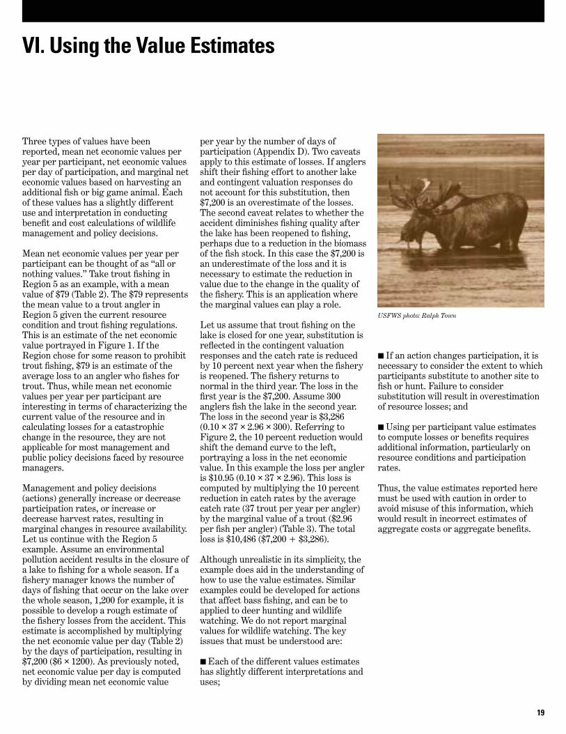
USFWS photo: Ralph Town

Net economic values represent the valuesabove and beyond what participantsactually spend to participate in anactivity. This value information can beused to assess the current value ofparticipation in these activities. Marginalvalues can be used to compute benefits orcosts of increasing or decreasing theavailability of selected wildlife resources.Marginal values provide a starting pointfor resource managers evaluatingchanges in resource availability, whetherit is a planned improvement or anunforeseen change.

Given the groupings of data reportedhere, we suggest wildlife managers useestimates from groups that include theirstates. There is no clear guidance as towhich groupings of states best representvalue estimates. We leave this decision towildlife managers to choose the groupingthey feel best represents conditions intheir state.

20

VII. Concluding Comments

USFWS photo: Luther Goldman

American Sport Fishing Association.1998. “The Economic Importance ofSport Fishing.” 1033 North Fairfax St.,Alexandria, VA.

Bishop, Richard C. 1984. “EconomicValues Defined.” In Valuing Wildlife:Economic and Social Perspectives, D.F.Decker and G.R. Goff (eds), WestviewPress, Boulder, CO.

Bishop, Richard C., Thomas A.Heberlein, and Mary Jo Kealy. 1983.“Contingent Valuation of EnvironmentalAssets: Comparisons With a SimulatedMarket.” Natural Resources Journal23:619-633.

Boyle, Kevin J. 1990. “Design ofContingent-Valuation Questions for the1991 National Survey of Fishing,Hunting, and Wildlife-AssociatedRecreation: Final Report.” Report toU.S. Fish and Wildlife Service.

Boyle, Kevin J., and Richard C. Bishop.1988. “Welfare Measurements UsingContingent Valuation: A Comparison ofTechniques.” American Journal ofAgricultural Economics70(February):20-28.

Cameron, Trudy Ann, and Michell D.James. 1987. “Efficient EstimationMethods for Use with Closed-EndedContingent Valuation Survey Data.”Review of Economics and Statistics69(May):269-276.

Cameron, Trudy Ann. 1988. “A NewParadigm for Valuing Non-Market GoodsUsing Referendum Data: MaximumLikelihood Estimation by CensoredLogistic Regression.” Journal ofEnvironmental Economics andManagement 15(September):355-379.

Cameron, Trudy Ann. 1991. “IntervalEstimates of Non-Market ResourceValues From Referendum ContingentValuation Surveys.” Land Economics67(November):413-421.

Cooper, Joseph C. 1993. “Optimal BidSelection for Dichotomous ChoiceContingent Valuation Surveys.” Journalof Environmental Economics andManagement 24(January):25-40.

Cooper, Joseph. 1994. “A Comparison ofApproaches to Calculating ConfidenceIntervals for Benefit Measures fromDichotomous Choice ContingentValuations Surveys.” Land Economics70(February):111-122.

Duffield, John W., and David A.Patterson. 1991. “Inference and OptimalDesign for a Welfare Measure inDichotomous Choice ContingentValuation.” Land Economics67(May):225-239.

Freeman, A. Myrick. 1993. TheMeasurement of Environmental andResource Values: Theory and Methods. Resources for the Future,Washington, DC.

Greene, William, H. 1992. LimdepVersion 6.0: User’s Manual andReference Guide. Bellport, New York.Econometric Software, Inc.

Hanemann, W. Michael. 1984. “WelfareEvaluations in Contingent ValuationExperiments with Discrete ResponseData.” American Journal of AgricultureEconomics 66(August):332-341.

Hanemann, W. Michael. 1989. “WelfareEvaluations in Contingent ValuationExperiments with Discrete ResponseData: Reply.” American Journal ofAgriculture Economics71(November):1056-1061.

Johnston, J. 1984. Econometric Methods.Third Edition, McGraw-Hill, Inc.

Judge, G., W. Griffiths, R. Hill, H.Lutkepohl, and T. Lee. 1985. The Theoryand Practice of Econometrics. SecondEdition. John Wiley and Sons, Inc.

Loomis, John B., George L. Peterson,and Cindy S. Sorg. 1984. “A Field Guideto Wildlife Economic Analysis.”Transactions of the Fourty-ninth NorthAmerican and Natural ResourcesConference: 315-324.

McCollum, Daniel W., George L.Peterson, and Cindy S. Swanson. 1992. “AManagers Guide to the Valuation ofNonmarket Resources: What Do YouReally Want to Know?” In ValuingWildlife Resources in Alaska, G.L.Peterson, C.S. Swanson, D.W. McCollum,and M.H. Thomas, (eds), Westview Press,Boulder, CO.

McConnell, K.E. 1990. “Models forReferendum Data: The Structure ofDiscrete Choice Models for ContingentValuation.” Journal of EnvironmentalEconomic and Management18(January):19-34.

Mitchell, Robert C., and Richard J.Carson. 1989. Using Surveys to ValuePublic Goods: The Contingent ValuationMethod. Washington, D.C. Resources forthe Future.

Park, Timothy, John B. Loomis, andMichael Creel. 1991. “ConfidenceIntervals for Evaluating BenefitsEstimates from Dichotomous ChoiceContingent Valuation Studies.” LandEconomics 67(February):64-73.

Southwick Associates for theInternational Association of Fish andWildlife Agencies. “The EconomicImportance of Hunting.” 1033 NorthFairfax St., Alexandria, VA.

U.S. Fish and Wildlife Service. “1996National and State Economic Impacts ofWildlife Watching.” Report 96-1.Washington, DC.

21

References

22

Appendix AContingent-Valuation Sections from the 1996 National Survey of Fishing,Hunting, and Wildlife-Associated Recreation for Fishing (Bass, Trout,and Walleye), Hunting (Deer, Elk, and Moose), and Wildlife Watching

Fishing Economic Evaluation

In the next few questions, I will ask you about ALL your trips taken during the ENTIRE calendar year of 1996 to PRIMARILYfish for [trout/bass/walleye] in [state].

Sometimes you may take a [trout/bass/walleye] fishing trip where you are away from your home for one night or several nights.Other times, you may take a [trout/bass/walleye] fishing trip where you leave from and return to your home on the same day. Intotal, how many trips did you take to fish PRIMARILY for [trout/bass/walleye] during 1996 in [state]?

_______Trips taken (Allow 3 digits)

How many [trout/bass/walleye] did you catch during 1996 in [state]? We are asking for how trout/bass/walleye] you CAUGHT andwe ARE NOT asking for how many [trout/bass/walleye] you KEPT.

_______ (Allow 4 digits)

What was the average length in inches of the [trout/bass/walleye] you caught during 1996 in [state]?

_______ Inches (Allow 2 digits)

Some [trout/bass/walleye] fishing trips cost more than others. For example, on a long trip you may spend money for food, travel,and lodging. On a short trip, where you may only fish for a few hours, you may only spend money for gas. How much did [yourtrip/an average trip] cost you during 1996 where you fished PRIMARILY for [trout/bass/walleye] in [state]?

$______ Cost per trip (Allow 6 digits)

Since you took [fill trips from above] [trout/bass/walleye] fishing trips and the average trip cost was $[fill average cost from above],this means that you spent about $[number trips • average cost per trip] in total for ALL of your trips during 1996 to fishPRIMARILY for [trout/bass/walleye] [state]. Would you say that this total cost is about right?

(1) ____Yes

(2) ____No

If No — How much would you say is the total cost of your [number of trips] trips to fish PRIMARILY for [trout/bass/walleye]during 1996 in [state]?

$______ Total Cost (Allow 8 digits)

Fishing expenses change over time. For example, gas prices rise and fall. Would you have taken any trips to fish PRIMARILY for[trout/bass/walleye] during 1996 in [state] if your total costs were $[bid value] more than the amount you just reported?

(1) ____Yes

(2) ____No

23

Hunting Economic Evaluation

In the next few questions, I will ask you about ALL your trips taken during the ENTIRE calendar year of 1996 PRIMARILY tohunt [deer/elk/moose] in [state].

Sometimes you may take [a/an] [deer/elk/moose] hunting trip where you are away from your home for one night or several nights.Other times, you may take [a/an] [deer/elk/moose] hunting trip where you leave from and return to your home on the same day. Intotal, how many trips did you take PRIMARILY to hunt [deer/elk/moose] during 1996 in [state]?

_______ Trips (Allow 3 digits)

Did you bag [buck deer/bull elk/bull moose] in 1996 in [state]?

(1) ____Yes

(2) ____No

(designated deer states only)

Some states allow hunters to bag more than one DEER. How many DEER did you bag during 1996 in [state]?

_______ Deer (Allow 2 digits)

Did you bag a [buck/bull elk/bull moose] in 1996 in [state]?

(1) ____Yes

(2) ____No

Some [deer/elk/moose] hunting trips cost more than others. For example, on a long trip you may spend money for food, travel, and lodging. On a short trip, where you may only hunt for a few hours, you may only spend money for gas. How much did [your trip/an average trip] cost you during 1996 when you went PRIMARILY to hunt [deer/elk/moose] in [state]?

$______ per trip (Allow 6 digits)

Since you took [fill trips from above] [deer/elk/moose] hunting trips and the average trip cost was $[fill average cost from above],this means that you spent about $ [number trips * average cost per trip] in total for ALL of your trips during 1996 PRIMARILYto hunt [deer/elk/moose] in [state]. Would you say that this total cost is about right?

(1) ____Yes

(2) ____No

If No — How much would you say is the total cost of your [fill trips from above] trips taken during 1996 PRIMARILY to hunt[deer/elk/moose] in [state]?

$______ Total Cost (Allow 8 digits)

Hunting expenses change over time. For example, gas prices rise and fall. Would you have taken any trips PRIMARILY to hunt[deer/elk/moose] during 1996 in [state] if your total [deer/elk/moose] hunting costs were $ [bid value] more than the amount youjust reported?

(1) ____Yes

(2) ____No

Wildlife Watching

In the next few questions, I will ask you about ALL your trips taken for the PRIMARY PURPOSE of observing, photographing,or feeding wildlife during the ENTIRE calendar year of 1996 in [state].

In your [current and previous interview] you reported taking [fill trips] [trip/trips] of at least one mile for the PRIMARYPURPOSE of observing, photographing, or feeding wildlife in [state]. Is that correct?

(1) ____Yes

(2) ____No

If No — How many trips of at least one mile did you take for the PRIMARY PURPOSE of observing, photographing, or feedingwildlife in [state] during 1996?

_______ (Allow 3 digits)

In your [current and previous interview], you reported that you spent $[fill trip expenditures] in total for [your trip/all of yourtrips] during 1996 where your PRIMARY PURPOSE was to observe, photograph, or feed wildlife in [state]. Would you say thatthis total cost is about right?

(1) ____Yes

(2) ____No

If No — How much would you say is the total cost of your [fill trips] [trip/trips] during 1996 where your PRIMARY PURPOSEwas to observe, photograph, or feed wildlife in [state]?

$______ Total Cost (Allow 8 digits)

Wildlife watching expenses change over time. For example, gas prices rise and fall. Would you have taken any trips during 1996 forthe PRIMARY PURPOSE of observing, photographing, or feeding wildlife in [state] if your total costs were $ [bid value] morethan the amount you just reported?

(1) ____Yes

(2) ____No

24

25

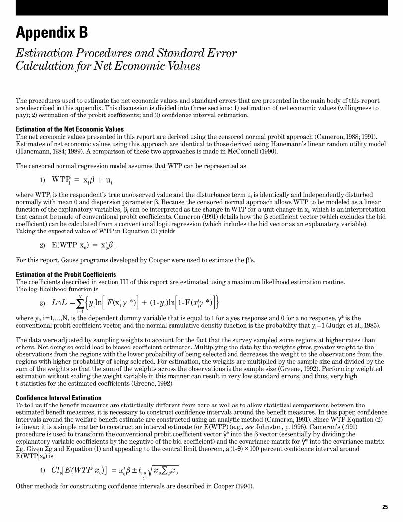
The procedures used to estimate the net economic values and standard errors that are presented in the main body of this reportare described in this appendix. This discussion is divided into three sections: 1) estimation of net economic values (willingness topay); 2) estimation of the probit coefficients; and 3) confidence interval estimation.

Estimation of the Net Economic ValuesThe net economic values presented in this report are derived using the censored normal probit approach (Cameron, 1988; 1991).Estimates of net economic values using this approach are identical to those derived using Hanemann’s linear random utility model(Hanemann, 1984; 1989). A comparison of these two approaches is made in McConnell (1990).

The censored normal regression model assumes that WTP can be represented as

1)

where WTPi is the respondent’s true unobserved value and the disturbance term ui is identically and independently disturbednormally with mean 0 and dispersion parameter β. Because the censored normal approach allows WTP to be modeled as a linearfunction of the explanatory variables, βi can be interpreted as the change in WTP for a unit change in xi, which is an interpretationthat cannot be made of conventional probit coefficients. Cameron (1991) details how the β coefficient vector (which excludes the bidcoefficient) can be calculated from a conventional logit regression (which includes the bid vector as an explanatory variable).Taking the expected value of WTP in Equation (1) yields

2)

For this report, Gauss programs developed by Cooper were used to estimate the β’s.

Estimation of the Probit CoefficientsThe coefficients described in section III of this report are estimated using a maximum likelihood estimation routine. The log-likelihood function is

3)

where yi, i=1,…,N, is the dependent dummy variable that is equal to 1 for a yes response and 0 for a no response, γ* is theconventional probit coefficient vector, and the normal cumulative density function is the probability that yi=1 (Judge et al., 1985).

The data were adjusted by sampling weights to account for the fact that the survey sampled some regions at higher rates thanothers. Not doing so could lead to biased coefficient estimates. Multiplying the data by the weights gives greater weight to theobservations from the regions with the lower probability of being selected and decreases the weight to the observations from theregions with higher probability of being selected. For estimation, the weights are multiplied by the sample size and divided by thesum of the weights so that the sum of the weights across the observations is the sample size (Greene, 1992). Performing weightedestimation without scaling the weight variable in this manner can result in very low standard errors, and thus, very high t-statistics for the estimated coefficients (Greene, 1992).

Confidence Interval EstimationTo tell us if the benefit measures are statistically different from zero as well as to allow statistical comparisons between theestimated benefit measures, it is necessary to construct confidence intervals around the benefit measures. In this paper, confidenceintervals around the welfare benefit estimate are constructed using an analytic method (Cameron, 1991). Since WTP Equation (2)is linear, it is a simple matter to construct an interval estimate for E(WTP) (e.g., see Johnston, p. 1996). Cameron’s (1991)procedure is used to transform the conventional probit coefficient vector γ̂* into the β vector (essentially by dividing theexplanatory variable coefficients by the negative of the bid coefficient) and the covariance matrix for γ̂* into the covariance matrixΣg. Given Σg and Equation (1) and appealing to the central limit theorem, a (1-θ) × 100 percent confidence interval aroundE(WTP|x0) is

4)

Other methods for constructing confidence intervals are described in Cooper (1994).

Appendix BEstimation Procedures and Standard ErrorCalculation for Net Economic Values

26

Table C-1. Probit Equation Results for FishingExplanatory Variables

Region Constant Bid Catch Inch Resident Species n Chi-squared %(# Fish) (Length) Correct

Predictions

U.S. Fish and Wildlife Service Official Regions

Appendix CProbit Equation Results

26

-0.1399(0.2067)

-0.0010(0.0002)

0.0007(0.0003)

0.0546(0.0113)

-0.3505(0.1829)

665 762.97 63 1 (CA, ID, NV, OR,WA)

-0.7913(0.3811)

-0.0004(0.0006)

0.0010(0.0008)

0.0750(0.0143)

-0.5988(0.2153)

0.2833(0.1736)

356 436.20 63 2 (AZ, NM, OK,TX)

-0.1572(0.3330)

-0.0021(0.0005)

0.0102(0.0020)

0.0102(0.0150)

0.2016(0.2325)

374 418.33 72 3 (IA, IL, IN, MO)

-0.4888(0.2260)

-0.0008(0.0003)

0.0029(0.0005)

0.0481(0.0091)

-0.2342(0.1235)

845 1015.48 67 4 (AL, AR, FL,GA, KY, LA, MS,NC, SC, TN)

0.4032(0.2136)

-0.0021(0.0003)

0.0061(0.0008)

0.0235(0.0085)

-0.4225(0.1139)

-0.3431(0.1017)

1118 1228.33 70 5 (CT, DE, MA,MD, ME, MY,NH, NJ, PA, RI,VA, VT, WV)

0.4048(0.2674)

-0.0023(0.0007)

0.0060(0.0009)

0.0123(0.0092)

-0.3777(0.1038)

0.1488

(0.1274)

899 1140.54 65 6 (CO, KS, MT,NE, UT, WY)

3.6076(2.1062)

-0.0120(0.0055)

0.0028(0.0023)

0.0920(0.0249)

-0.4183(0.2978)

104 115.36 65 7 (AK)

U.S. Bureau of the Census Regions

-0.3482(0.2713)

-0.0009(0.0002)

0.0006(0.0004)

0.0592(0.0131)

-0.2750(0.2443)

499 552.91 68 Pacific (AK, CA, OR,WA)

0.2398(0.1991)

-0.0011(0.0005)

0.0030(0.0005)

0.0257(0.0076)

-0.4312(0.0834)

1244 1626.55 61 Mountain (AZ, CO,ID, MT, NM, NV,UT, WY)

0.0580(0.3118)

-0.0017(0.0005)

0.0101(0.0021)

0.0172(0.0154)

-0.2986(0.2215)

322 386.15 66 West North Central(IA, KS, MO,NE)

0.9510(1.1877)

-0.0051(0.0021)

0.0074(0.0024)

0.0009(0.0230)

0.8202(0.4861)

194 202.81 74 East North Central(IN, IL)

-0.2095(0.3738)

-0.0019(0.0006)

0.0071(0.0021)

0.0152(0.0178)

-0.2123(0.2739)

245 251.15 72 Middle Atlantic (NJ,NY, PA)

0.0274(0.3719)

-0.0015(0.0008)

0.0059(0.0012)

0.0292(0.0113)

-0.4920(0.1345)

0.0897(0.1708)

612 721.97 68 New England (CT,MA, ME, NH,RI, VT)

-1.1346(0.4599)

-0.0006(0.0006)

0.0012(0.0007)

0.0887(0.0166)

0.1281(0.2534)

262 307.54 68 West South Central(AR, LA, OK,TX)

0.0461(0.6094)

-0.0009(0.0010)

0.0044(0.0010)

0.0315(0.0146)

-0.4870(0.1858)

378 466.56 64 East South Central(AL, KY, MS,TN)

-0.4282(0.2512)

-0.0008(0.0003)

0.0044(0.0007)

0.0410(0.0114)

-0.3610(0.1586)

605 697.39 69 South Atlantic (DE,FL, GA, MD,NC, SC, VA, WV)

27

0.0467(0.2016)

-0.0020(0.0004)

0.0068(0.0013)

0.0177(0.0104)

-0.3836(0.1454)

657 715.67 71 New England (CT,ME, NH, NJ,NY, PA, VT)

-0.3197(0.2787)

-0.0009(0.0002)

0.0009(0.0004)

0.0519(0.0131)

-0.2401(0.2607)

500 558.42 66 Western Trout (AR,CA, NV, OR, WA)

0.1965(0.2084)

-0.0010(0.0005)

0.0029(0.0006)

0.0275(0.0081)

-0.4243(0.0865)

1139 1491.58 62 Mountain Trout (AZ,CO, ID, MT, NM,UT, WY)

0.0365(0.2038)

-0.0018(0.0003)

0.0066(0.0008)

0.0306(0.0090)

-0.2433(0.1250)

1088 1256.03 69 Northern Bass (DE,IA, IL, IN, KS,KY, MA, MD, MO,NE, RI, VA, WV)

-0.7107(0.2321)

-0.0006(0.0003)

0.0022(0.0005)

0.0569(0.0093)

-0.1221(0.1346)

838 1016.00 66 Southern Bass (AL, AR,FL, GA, LA, MS, NC,OK, SC, TN, TX)

0.1575(0.0780)

-0.0003(0.0002)

-0.0014(0.0004)

-0.0006(0.0010)

-0.0005(0.0021)

516 665.41 72 Walleye (MI, MN,ND, OH, SD, WI)

Table C-2. Probit Equation Results for HuntingExplanatory Variables

Region Constant Bid # of Sex of Hunt Resident n Chi- %Animals Animal Other squared CorrectBagged1 Bagged Big Game Prediction

U.S. Fish and Wildlife Service Official Regions (Deer Hunting)

2 (AZ, NM, OK, TX)

3 (IA, IL, IN, MI,MN, MO, OH, WI)

4 (AL, AR, FL, GA,KY, LA, MS, NC,SC, TN)

5 (CT, DE, MA, MD,ME, NH, NJ, NY,PA, RI, VA, VT,WV)

6 (KS, ND, NE, SD,UT, WY)

U.S. Bureau of the Census Regions (Deer Hunting)

Pacific (CA, WA)

Mountain (AZ, NM, NV,UT)

West North Central(IA, KS, MN, MO,NE, NE, SD)

Table C1. Probit Equation Results for Fishing (continued)Explanatory Variables

Region Constant Bid Catch Inch Resident n Chi-squared %(# Fish) (Length) Correct

Predictions

1 (CA, NV, WA) -1.3252(1.6510)

-0.0003(0.0008)

0.4180(0.4863)

-0.4925(0.5755)

0.3326(0.3214)

0.6408(1.5570)

109 109.43 73

0.0281(0.7567)

-0.0006(0.0011)

0.2400(0.0975)

-0.2528(0.2583)

0.4715(0.2083)

-0.2392(0.4371)

222 283.21 65

0.1164(0.2586)

-0.0014(0.0004)

0.2781(0.0717)

-0.1149(0.1330)

0.3026(0.1414)

-0.0079(0.2030)

736 948.92 64

-0.4147(0.3885)

-0.0004(0.0006)

0.0694(0.0350)

0.3464(0.1247)

0.2548(0.1089)

0.2212(0.1477)

738 961.71 63

-0.1319(0.1776)

-0.0007(0.0003)

0.2600(0.0589)

0.0682(0.1173)

0.2966(0.0794)

-0.1212(0.1090)

1147 1461.04 63

2.0845(0.4083)

-0.0040(0.0008)

0.1582(0.1365)

-0.0996(0.1835)

0.3451(0.2044)

-1.1252(0.2953)

390 492.38 60

-0.3769(2.4449)

-0.0004(0.0010)

0.5061(0.6398)

-0.7945(0.7467)

0.4266(0.3801)

-0.3033(2.4121)

79 76.22 80

0.9854(0.3586)

-0.0012(0.0005)

0.4064(0.5962)

-0.4432(0.6074)

-0.0674(0.2691)

-0.7066(0.2924)

209 277.07 58

0.0844(0.3226)

-0.0021(0.0005)

0.2254(0.0838)

-0.0651(0.1440)

0.4560(0.1463)

0.1627(0.2650)

591 750.93 62

28

East North Central(IN, IL, MI, OH,WI)

Middle Atlantic (NJ,NY, PA)

New England (CT, MA,ME, NH, RI, VT)

West South Central(AR, LA, OK, TX)

East South Central(AL, KY, MS, TN)

South Atlantic (DE, FL,GA, MD, NC, SC,VA, WV)

U.S. Fish and Wildlife Service Deer Regions

Pacific (CA, NV, WA)

West Southwest (AZ,NM, UT)

East Southwest (OK,TX)

Plains (IA, KS, MO,ND, NE, SD)

Great Lakes (IN, IL,MI, MN, OH, WI)

Middle Atlantic (DE,MD, NJ, NY, PA)

Table C2. Probit Equation Results for Hunting (continued)Explanatory Variables

Region Constant Bid # of Sex of Hunt Resident n Chi- %Animals Animal Other squared CorrectBagged1 Bagged Big Game Prediction

-1.3255(1.6513)

-0.0003(0.0008)

0.4180(0.4862)

-0.4926(0.5755)

0.3326(0.3214)

0.6410(1.5574)

109 109.42 73

1.4486(0.4264)

-0.0011(0.0007)

0.8973(0.7388)

-0.8954(0.7549)

-0.2050(0.2972)

-1.2314(0.3725)

179 229.16 60

0.2233(1.4276)

-0.0009(0.0024)

0.2330(0.1275)

-0.2353(0.3493)

0.5679(0.2822)

-0.2916(0.5878)

121 152.86 66

0.3818(0.3222)

-0.0023(0.0005)

0.3212(0.0928)

-0.2260(0.1512)

0.5163(0.1401)

-0.0918(0.2666)

496 615.39 63

0.1218(0.3095)

-0.0013(0.0005)

0.2563(0.0827)

-0.0806(0.1559)

0.2172(0.1836)

-0.0089(0.2361)

554 720.68 65

-1.1185(0.3911)

-0.0000(0.0006)

0.4417(0.1318)

0.0022(0.2233)

0.4205(0.1366)

0.3221(0.2287)

406 480.32 68

0.5148(0.2078)

-0.0012(0.0003)

-0.1078(0.1664)

0.2574(0.2484)

0.5354(0.1452)

-0.2292(0.1513)

467 611.02 60

-0.3270(0.2330)

-0.0003(0.0004)

0.0836(0.0315)

0.2761(0.1055)

0.2200(0.0896)

0.0434(0.1175)

1013 1330.17 63

1.4414(0.3910)

-0.0027(0.0008)

-0.2220(0.1461)

0.6356(0.1831)

0.5716(0.1620)

-0.6592(0.2573)

421 515.75 60

3.7033(3.7240)

-0.0066(0.0054)

0.9864(0.4582)

-0.4053(0.5117)

0.2666(0.3191) 75 86.53 65

0.3336(0.3352)

-0.0016(0.0005)

0.2938(0.0906)

-0.1648(0.1688)

0.2059(0.1934)

-0.0702(0.2497)

457 590.38 65

-1.3150(0.5457)

0.0001(0.0010)

0.5447(0.1617)

-0.1577(0.2726)

0.4584(0.1582)

0.4617(0.2873)

301 350.62 70

0.5148(0.2078)

-0.0012(0.0003)

-0.1078(0.1664)

0.2574(0.2484)

0.5354(0.1452)

-0.2291(0.1513)

467 611.02 60

-1.0260(0.7767)

0.0008(0.0012)

0.1914(0.0892)

0.0024(0.2383)

0.4684(0.2007)

0.0736(0.3746)

244 313.43 61

-0.0367(0.5009)

-0.0012(0.0007)

0.1716(0.0555)

0.2269(0.1817)

0.2047(0.1612)

0.1307(0.1866)

375 454.20 67

-0.2535(0.2548)

0.0001(0.0004)

0.0311(0.0401)

0.2727(0.1331)

0.1768(0.1090)

-0.1735(0.1512)

619 834.23 61

New England (CT, MA,ME, NH, RI, VT)

South East (AL, AR,FL, GA, KY, LA,MS, NC, SC, TN,VA, WV)

Other Big Game Species Elk Region (CO, ID,

MT, OR, WY)

Moose Region (AK)

1 Respondents were asked if they bagged a moose or elk but not the number bagged so for the elk and moose regions this variable equals 0 or 1, where 1 meansthey bagged an animal.

29

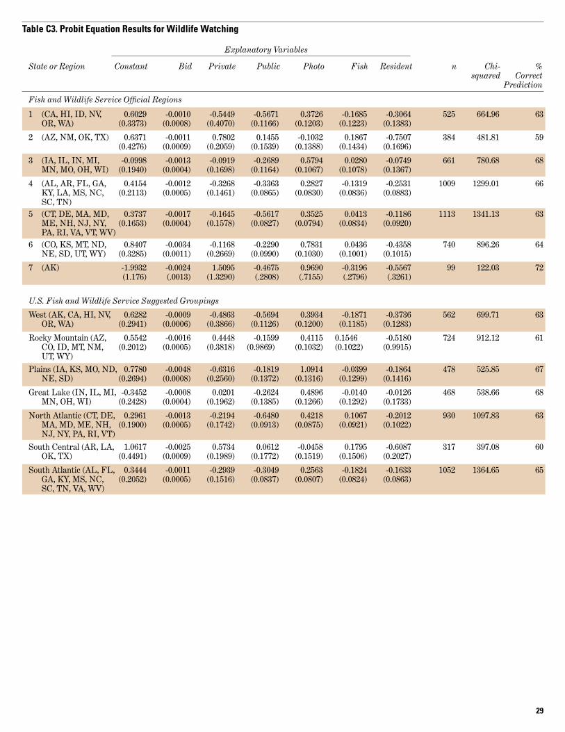
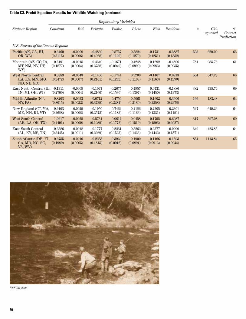
Table C3. Probit Equation Results for Wildlife Watching

Explanatory Variables

State or Region Constant Bid Private Public Photo Fish Resident n Chi- %squared Correct

Prediction

Fish and Wildlife Service Official Regions

0.6029(0.3373)

-0.0010(0.0008)

-0.5449(0.4070)

-0.5671(0.1166)

0.3726(0.1203)

-0.1685(0.1223)

-0.3064(0.1383)

525 664.96 63 1 (CA, HI, ID, NV, OR, WA)

0.6371(0.4276)

-0.0011(0.0009)

0.7802(0.2059)

0.1455(0.1539)

-0.1032(0.1388)

0.1867(0.1434)

-0.7507(0.1696)

384 481.81 59 2 (AZ, NM, OK, TX)

-0.0998(0.1940)

-0.0013(0.0004)

-0.0919(0.1698)

-0.2689(0.1164)

0.5794(0.1067)

0.0280(0.1078)

-0.0749(0.1367)

661 780.68 68 3 (IA, IL, IN, MI, MN, MO, OH, WI)

0.4154(0.2113)

-0.0012(0.0005)

-0.3268(0.1461)

-0.3363(0.0865)

0.2827(0.0830)

-0.1319(0.0836)

-0.2531(0.0883)

1009 1299.01 66 4 (AL, AR, FL, GA,KY, LA, MS, NC, SC, TN)

0.3737(0.1653)

-0.0017(0.0004)

-0.1645(0.1578)

-0.5617(0.0827)

0.3525(0.0794)

0.0413(0.0834)

-0.1186(0.0920)

1113 1341.13 63 5 (CT, DE, MA, MD,ME, NH, NJ, NY,PA, RI, VA, VT, WV)

0.8407(0.3285)

-0.0034(0.0011)

-0.1168(0.2669)

-0.2290(0.0990)

0.7831(0.1030)

0.0436(0.1001)

-0.4358(0.1015)

740 896.26 64 6 (CO, KS, MT, ND,NE, SD, UT, WY)

-1.9932(1.176)

-0.0024(.0013)

1.5095(1.3290)

-0.4675(.2808)

0.9690(.7155)

-0.3196(.2796)

-0.5567(.3261)

99 122.03 72 7 (AK)

U.S. Fish and Wildlife Service Suggested Groupings

0.6282(0.2941)

-0.0009(0.0006)

-0.4863(0.3866)

-0.5694(0.1126)

0.3934(0.1200)

-0.1871(0.1185)

-0.3736(0.1283)

562 699.71 63 West (AK, CA, HI, NV,OR, WA)

0.5542(0.2012)

-0.0016(0.0005)

0.4448(0.3818)

-0.1599(0.9869)

0.4115(0.1032)

0.1546(0.1022)

-0.5180(0.9915)

724 912.12 61 Rocky Mountain (AZ,CO, ID, MT, NM, UT, WY)

0.7780(0.2694)

-0.0048(0.0008)

-0.6316(0.2560)

-0.1819(0.1372)

1.0914(0.1316)

-0.0399(0.1299)

-0.1864(0.1416)

478 525.85 67 Plains (IA, KS, MO, ND,NE, SD)

-0.3452(0.2428)

-0.0008(0.0004)

0.0201(0.1962)

-0.2624(0.1385)

0.4896(0.1266)

-0.0140(0.1292)

-0.0126(0.1733)

468 538.66 68 Great Lake (IN, IL, MI,MN, OH, WI)

0.2961(0.1900)

-0.0013(0.0005)

-0.2194(0.1742)

-0.6480(0.0913)

0.4218(0.0875)

0.1067(0.0921)

-0.2012(0.1022)

930 1097.83 63 North Atlantic (CT, DE,MA, MD, ME, NH,NJ, NY, PA, RI, VT)

1.0617(0.4491)

-0.0025(0.0009)

0.5734(0.1989)

0.0612(0.1772)

-0.0458(0.1519)

0.1795(0.1506)

-0.6087(0.2027)

317 397.08 60 South Central (AR, LA,OK, TX)

0.3444(0.2052)

-0.0011(0.0005)

-0.2939(0.1516)

-0.3049(0.0837)

0.2563(0.0807)

-0.1824(0.0824)

-0.1633(0.0863)

1052 1364.65 65 South Atlantic (AL, FL,GA, KY, MS, NC, SC, TN, VA, WV)

30

U.S. Bureau of the Census Regions

0.6469(0.3115)

-0.0009(0.0006)

-0.4869(0.4028)

-0.5757(0.1190)

0.3824(0.1270)

-0.1731(0.1251)

-0.3887(0.1352)

505 629.00 63 Pacific (AK, CA, HI, OR, WA)

0.5191(0.1877)

-0.0015(0.0004)

0.4340(0.3738)

-0.1671(0.0949)

0.4248(0.0990)

0.1292(0.0983)

-0.4896(0.0955)

781 985.76 61 Mountain (AZ, CO, IA,MT, NM, NV, UT,WY)

0.5383(0.2472)

-0.0043(0.0007)

-0.1466(0.2161)

-0.1744(0.1252)

0.9200(0.1193)

-0.1467(0.1163)

0.0213(0.1290)

564 647.28 66 West North Central (IA, KS, MN, MO,ND, NE, SD)

-0.1311(0.2700)

-0.0009(0.0004)

-0.1047(0.2160)

-0.2675(0.1530)

0.4957(0.1397)

0.0731(0.1450)

-0.1886(0.1973)

382 438.74 69 East North Central (IL,IN, MI, OH, WI)

0.8203(0.8015)

-0.0033(0.0022)

-0.0712(0.3739)

-0.4750(0.2281)

0.5061(0.2180)

0.1602(0.2258)

-0.3606(0.2978)

166 183.48 64 Middle Atlantic (NJ, NY, PA)

0.9103(0.2688)

-0.0029(0.0008)

-0.1950(0.2572)

-0.7464(0.1183)

0.4186(0.1166)

-0.2305(0.1331)

-0.2301(0.1191)

547 649.26 64 New England (CT, MA,ME, NH, RI, VT)

1.0617(0.4491)

-0.0025(0.0009)

0.5734(0.1989)

0.0612(0.1772)

-0.0458(0.1519)

0.1795(0.1506)

-0.6087(0.2027)

317 397.08 60 West South Central (AR, LA, OK, TX)

0.2586(0.3445)

-0.0018(0.0011)

-0.1777(0.2269)

-0.2231(0.1523)

0.5262(0.1433)

-0.2377(0.1442)

-0.0990(0.1571)

349 423.85 64 East South Central (AL, KY, MS, TN)

0.3755(0.1989)

-0.0010(0.0005)

-0.2253(0.1815)

-0.3930(0.0916)

0.1900(0.0891)

-0.1166(0.0913)

-0.1593(0.0944)

854 1113.84 65 South Atlantic (DE, FL,GA, MD, NC, SC,VA, WV)

Table C3. Probit Equation Results for Wildlife Watching (continued)

Explanatory Variables

State or Region Constant Bid Private Public Photo Fish Resident n Chi- %squared Correct

Prediction

USFWS photo

31

Table D1. Average Days per Year for Fishing

Region Species Valued Average Days/Year

U.S. Fish and Wildlife Service Regions 1 (CA, ID, NV, OR, WA) Trout 10.7 2 (AZ, NM, OK, TX) Bass & Trout 11.0

(OH, TX) Bass 11.4 (AZ, NM) Trout 10.8

3 (IA, IL, IN, MO) Bass 14.4 4 (AL, AR, FL, GA, KY, LA, MS, NC, SC, TN) Bass 16.4 5 (CT, DE, MA, MD, ME, NH, NJ, NY, PA, RI, VA, VT, WV) Bass & Trout 15.0

(DE, MA, MD, RI, VA, WV) Bass 16.8 (CT, ME, NH, NJ, NY, PA, VT) Trout 13.7

6 (CO, KS, MT, NE, UT, WY) Bass & Trout 19.3 (KS, NE) Bass 19.3 (CO, MT, UT, WY) Trout 10.1

7 (AK) Trout 10.0

U.S. Bureau of the Census Regions Pacific (AK, CA, OR, WA) Trout 11.3 Mountain (AZ, CO, ID, MT, NM, NV, UT, WY) Trout 10.1 West North Central (IA, KS, MO, NE) Bass 17.4 East North Central (IL, IN) Bass 15.6 Middle Atlantic (NJ, NY, PA) Trout 13.0 New England (CT, MA, ME, NH, RI, VT) Bass & Trout 15.6 (MA, RI) Bass 18.4 (CT, ME, NH, VT) Trout 14.2 West South Central (AR, LA, OK, TX) Bass 13.8 East South Central (AL, KY, MS, TN) Bass 16.3 South Atlantic (DE, FL, GA, MD, NC, SC, VA, WV) Bass 16.1

U.S. Fish and Wildlife Service Bass Regions Northern (DE, IA, IL, IN, KS, KY, MA, MD, MO, NE, RI, VA, WV) Bass 16.2 Southern (AL, AR, FL, GA, LA, MS, NC, OK, SC, TN, TX) Bass 15.7

U. S. Fish and Wildlife Service Trout Regions Western (AR, CA, NV, OR, WA) Trout 11.3 Mountain (AZ, CO, ID, MT, NM, UT, WY) Trout 10.1 Northeast (CT, ME, NH, NJ, NY, PA, VT) Trout 13.7

U.S. Fish and Wildlife Service Walleye RegionsWalleye Region (MI, MN, ND, OH, SD, WI) Walleye 16.3

Appendix DAverage Days of Participation

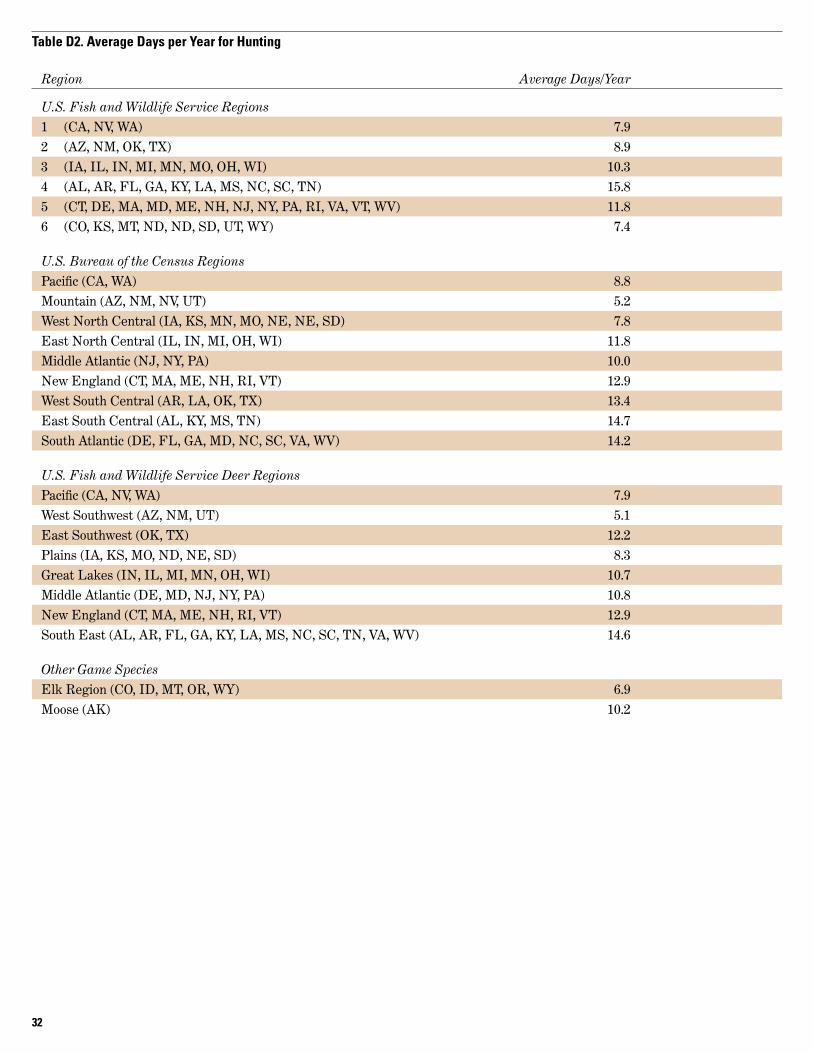
32

Table D2. Average Days per Year for Hunting

Region Average Days/Year

U.S. Fish and Wildlife Service Regions 1 (CA, NV, WA) 7.9 2 (AZ, NM, OK, TX) 8.9 3 (IA, IL, IN, MI, MN, MO, OH, WI) 10.3 4 (AL, AR, FL, GA, KY, LA, MS, NC, SC, TN) 15.8 5 (CT, DE, MA, MD, ME, NH, NJ, NY, PA, RI, VA, VT, WV) 11.8 6 (CO, KS, MT, ND, ND, SD, UT, WY) 7.4

U.S. Bureau of the Census RegionsPacific (CA, WA) 8.8 Mountain (AZ, NM, NV, UT) 5.2 West North Central (IA, KS, MN, MO, NE, NE, SD) 7.8 East North Central (IL, IN, MI, OH, WI) 11.8 Middle Atlantic (NJ, NY, PA) 10.0 New England (CT, MA, ME, NH, RI, VT) 12.9 West South Central (AR, LA, OK, TX) 13.4 East South Central (AL, KY, MS, TN) 14.7 South Atlantic (DE, FL, GA, MD, NC, SC, VA, WV) 14.2

U.S. Fish and Wildlife Service Deer Regions Pacific (CA, NV, WA) 7.9 West Southwest (AZ, NM, UT) 5.1 East Southwest (OK, TX) 12.2 Plains (IA, KS, MO, ND, NE, SD) 8.3 Great Lakes (IN, IL, MI, MN, OH, WI) 10.7 Middle Atlantic (DE, MD, NJ, NY, PA) 10.8 New England (CT, MA, ME, NH, RI, VT) 12.9 South East (AL, AR, FL, GA, KY, LA, MS, NC, SC, TN, VA, WV) 14.6

Other Game SpeciesElk Region (CO, ID, MT, OR, WY) 6.9 Moose (AK) 10.2

33

Table D3. Average Days per Year for Wildlife Watching

Region Average Days/Year

U.S. Fish and Wildlife Service Regions 1 (CA, ID, NV, WA, OR) 11.5 2 (AZ, NM, OK, TX) 12.9 3 (IA, IL, IN, MI, MN, MO, OH, WI) 11.1 4 (AL, AR, FL, GA, KY, LA, MS, NC, SC, TN) 11.2 5 (CT, DE, MA, MD, ME, NH, NJ, NY, PA, RI, VA, VT, WV) 10.8 6 (CO, KS, MT, ND, NE, SD, UT, WY) 10.5 7 (AK) 20.2

U.S. Bureau of the Census RegionsPacific (AK, CA, HI, OR, WA) 13.9 Mountain (AZ, CO, IA, MT, NM, NV, UT, WY) 10.2 West North Central (IA, KS, MN, MO, ND, NE, SD) 11.1 East North Central (IL, IN, MI, OH, WI) 12.6 Middle Atlantic ( NJ, NY, PA) 8.5 New England (CT, MA, ME, NH, RI, VT) 11.6 West South Central (AR, LA, OK, TX) 13.4 East South Central (AL, KY, MS, TN) 12.2 South Atlantic (DE, FL, GA, MD, NC, SC, VA, WV) 10.0

U.S. Fish and Wildlife Service Suggested RegionsWest (WA, CA, OR, NV, HI, AK) 13.3 Rocky Mountain (ID, MT, WY, UT, CO, AZ, NM) 10.3 Plains (ND, SD, NE, KS, IA, MO) 11.4 Great Lake (MN, WI, IL, IN, MI, OH) 12.1 North Atlantic (MD, DE, PA, NJ, NY, CT, RI, MA, VT, NH, ME) 11.0 South Central (AR, LA, OK, TX) 13.4 South Atlantic (AL, FL, GA, KY, MS, NC, SC, TN, VA, WV) 10.4

34

Table E1. Censored Probit Marginal Coefficients for Fishing

Region Catch Inch Resident Species(# Fish) (Length)

U.S. Fish and Wildlife Service Regions1 (CA, ID, NV, OR, WA) 0.71 55.28 –354.722 (AZ, NM, OK, TX) –2.58 –199.22 1590.90 –752.723 (IA, IL, IN, MO) 4.84 4.85 96.144 (AL, AR, FL, GA, KY, LA, MS, NC, SC, TN) 3.81 64.04 –311.535 (CT, DE, MA, MD, ME, NH, NJ, NY, PA, RI, VA, VT, WV) 2.96 11.39 –204.84 –166.38

(DE, MA, MD, RI, VA, WV) 2.65 5.40 –165.65(CT, ME, NH, NJ, NY, PA, VT) 0.24 7.66 –34.81

U.S. Bureau of the Census RegionsPacific (AK, CA, OR, WA) 0.71 66.09 –306.92Mountain (AZ, CO, ID, MT, NM, NV, UT, WY) 2.75 23.11 –388.10West North Central (IA, KS, MO, NE) 6.05 10.29 –178.53East North Central (IL, IN) 1.44 0.17 160.69Middle Atlantic (NJ, NY, PA) 3.69 7.96 –110.95New England (CT, MA, ME, NH, RI, VT) 3.86 18.99 –319.62 58.26West South Central (AR, LA, OK, TX) 4.61 33.39 –516.53East South Central (AL, KY, MS, TN) 1.66 135.81 196.09South Atlantic (DE, FL, GA, MD, NC, SC, VA, WV) 5.86 54.97 –483.59

U.S. Fish and Wildlife Service Fishing RegionsNew England (CT, ME, NH, NJ, NY, PA, VT) 3.38 8.84 –192.02Western (AR, CA, NV, OR, WA) 0.78 59.15 –273.62Mountain (AZ, CO, ID, MT, NM, UT, WY) 2.81 26.50 –409.57All Bass States 3.32 45.19 –166.75Northern (DE, IA, IL, IN, KS, KY, MA, MD, MO, NE, RI, VA, WV) 3.60 16.55 –131.68Southern (AL, AR, FL, GA, LA, MS, NC, OK, SC, TN, TX) 3.53 92.32 –198.09Walleye (MI, MN, ND, OH, SD, WI) –4.67 –2.16 –1.78

Appendix ECensored Probit Marginal Coefficients

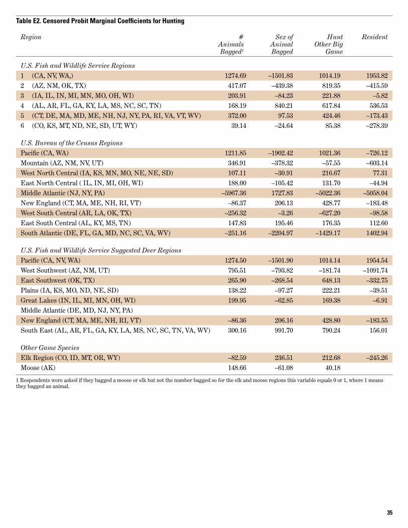
35

Table E2. Censored Probit Marginal Coefficients for Hunting

Region # Sex of Hunt ResidentAnimals Animal Other BigBagged1 Bagged Game

U.S. Fish and Wildlife Service Regions1 (CA, NV, WA,) 1274.69 –1501.83 1014.19 1953.822 (AZ, NM, OK, TX) 417.07 –439.38 819.35 –415.593 (IA, IL, IN, MI, MN, MO, OH, WI) 203.91 –84.23 221.88 –5.824 (AL, AR, FL, GA, KY, LA, MS, NC, SC, TN) 168.19 840.21 617.84 536.535 (CT, DE, MA, MD, ME, NH, NJ, NY, PA, RI, VA, VT, WV) 372.00 97.53 424.46 –173.436 (CO, KS, MT, ND, NE, SD, UT, WY) 39.14 –24.64 85.38 –278.39

U.S. Bureau of the Census RegionsPacific (CA, WA) 1211.85 –1902.42 1021.36 –726.12Mountain (AZ, NM, NV, UT) 346.91 –378.32 –57.55 –603.14West North Central (IA, KS, MN, MO, NE, NE, SD) 107.11 –30.91 216.67 77.31East North Central ( IL, IN, MI, OH, WI) 188.00 –105.42 131.70 –44.94Middle Atlantic (NJ, NY, PA) –5967.36 1727.83 –5022.36 –5058.04New England (CT, MA, ME, NH, RI, VT) –86.37 206.13 428.77 –183.48West South Central (AR, LA, OK, TX) –256.32 –3.26 –627.20 –98.58East South Central (AL, KY, MS, TN) 147.83 195.46 176.35 112.60South Atlantic (DE, FL, GA, MD, NC, SC, VA, WV) –251.16 –2204.97 –1429.17 1402.94

U.S. Fish and Wildlife Service Suggested Deer RegionsPacific (CA, NV, WA) 1274.50 –1501.90 1014.14 1954.54West Southwest (AZ, NM, UT) 795.51 –793.82 –181.74 –1091.74East Southwest (OK, TX) 265.90 –268.54 648.13 –332.75Plains (IA, KS, MO, ND, NE, SD) 138.22 –97.27 222.21 –39.51Great Lakes (IN, IL, MI, MN, OH, WI) 199.95 –62.85 169.38 –6.91Middle Atlantic (DE, MD, NJ, NY, PA)New England (CT, MA, ME, NH, RI, VT) –86.36 206.16 428.80 –183.55South East (AL, AR, FL, GA, KY, LA, MS, NC, SC, TN, VA, WV) 300.16 991.70 790.24 156.01

Other Game SpeciesElk Region (CO, ID, MT, OR, WY) –82.59 236.51 212.68 –245.26Moose (AK) 148.66 –61.08 40.18

1 Respondents were asked if they bagged a moose or elk but not the number bagged so for the elk and moose regions this variable equals 0 or 1, where 1 meansthey bagged an animal.

36

Table E3. Censored Probit Marginal Coefficients for Wildlife Watching

Region Private Public Photo Fish Resident

U.S. Fish and Wildlife Service Regions1 (CA, ID, HI, NV, WA, OR) –539.66 –561.69 368.99 –166.91 –303.512 (AZ, NM, OK, TX) 705.53 131.58 –93.33 168.80 –678.883 (IA, IL, IN, MI, MN, MO, OH, WI) –70.38 –205.87 443.63 21.47 –57.324 (AL, AR, FL, GA, KY, LA, MS, NC, SC, TN) –282.73 –290.94 244.60 –114.10 –218.985 (CT, DE, MA, MD, ME, NH, NJ, NY, PA,

RI, VA, VT, WV) –96.89 –330.76 207.57 24.30 –69.876 (CO, KS, MT, ND, NE, SD, UT, WY) –34.46 –67.56 231.05 12.85 –128.577 (AK) –626.24 193.93 –401.99 132.60 230.94

U.S. Bureau of the Census RegionsPacific (AK, CA, HI, OR, WA) –533.15 –630.43 418.79 –189.52 –425.66Mountain (AZ, CO, IA, MT, NM, NV, UT, WY) 293.63 –113.06 287.43 87.42 –331.29West North Central (IA, KS, MN, MO, ND,

NE, SD) –33.98 –40.44 213.29 –34.02 4.95East North Central (IL, IN, MI, OH, WI) –116.52 –297.62 551.55 81.29 –209.89Middle Atlantic (NJ, NY, PA) –2614.27 –4191.33 4179.42 2008.81 –1954.76New England (CT, MA, ME, NH, RI, VT) –68.24 –261.14 146.45 –80.64 –80.49West South Central (AR, LA, OK, TX) 233.36 24.90 –18.66 73.06 –247.74East South Central (AL, KY, MS, TN) –98.58 –123.76 291.91 –131.85 –54.89South Atlantic (DE, FL, GA, MD, NC, SC,

VA, WV) –220.78 –385.24 186.18 –114.25 –156.12

U.S. Fish and Wildlife Service Suggested RegionsWest (AK, CA, HI, NV, OR, WA) –534.73 –626.12 432.63 –205.79 –410.88Rocky Mountain (AZ, CO, ID, MT, NM, UT, WY) 283.54 –101.93 262.31 98.55 –330.17Plains (IA, KS, MO, ND, NE, SD) –132.24 –38.08 228.51 –8.36 –39.04Great Lake (IN, IL, MI, MN, OH, WI) 26.57 –347.36 648.23 –18.55 –16.64North Atlantic (CT, DE, MA, MD, ME, NH,

NJ, NY, PA, RI, VT) –167.61 –495.00 322.17 81.50 –153.69South Central (AR, LA, OK, TX) 233.36 24.90 –18.66 73.06 –247.74South Atlantic (AL, FL, GA, KY, MS, NC,

SC, TN, VA, WV) –267.22 –277.20 233.01 –165.79 –148.49

U.S. Department of the InteriorU.S. Fish & Wildlife ServiceDivision of EconomicsArlington, Virginia

http://www.fws.gov