18 gis applications to the basin-scale assessment of soil salinity

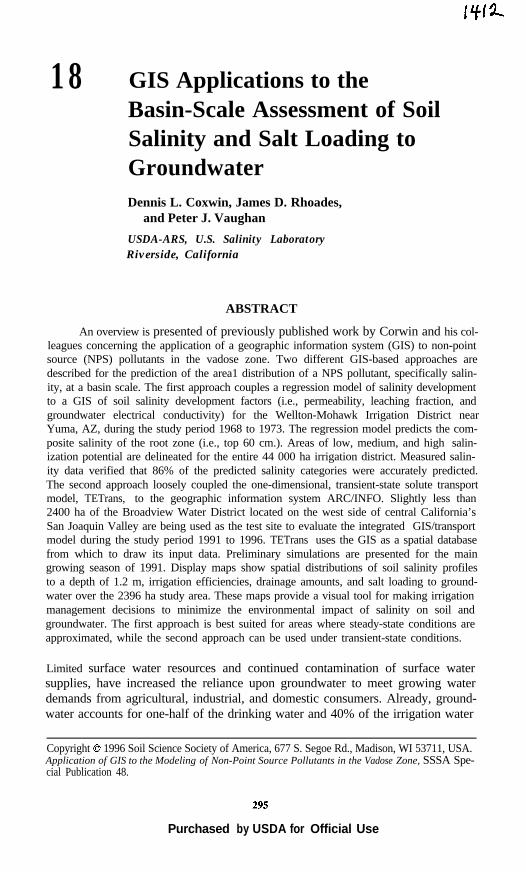
18 GIS Applications to theBasin-Scale Assessment of SoilSalinity and Salt Loading toGroundwaterDennis L. Coxwin, James D. Rhoades,

and Peter J. Vaughan

USDA-ARS, U.S. Salinity LaboratoryRiverside, California

ABSTRACT

An overview is presented of previously published work by Corwin and his col-leagues concerning the application of a geographic information system (GIS) to non-pointsource (NPS) pollutants in the vadose zone. Two different GIS-based approaches aredescribed for the prediction of the area1 distribution of a NPS pollutant, specifically salin-ity, at a basin scale. The first approach couples a regression model of salinity developmentto a GIS of soil salinity development factors (i.e., permeability, leaching fraction, andgroundwater electrical conductivity) for the Wellton-Mohawk Irrigation District nearYuma, AZ, during the study period 1968 to 1973. The regression model predicts the com-posite salinity of the root zone (i.e., top 60 cm.). Areas of low, medium, and high salin-ization potential are delineated for the entire 44 000 ha irrigation district. Measured salin-ity data verified that 86% of the predicted salinity categories were accurately predicted.The second approach loosely coupled the one-dimensional, transient-state solute transportmodel, TETrans, to the geographic information system ARC/INFO. Slightly less than2400 ha of the Broadview Water District located on the west side of central California’sSan Joaquin Valley are being used as the test site to evaluate the integrated GIS/transportmodel during the study period 1991 to 1996. TETrans uses the GIS as a spatial databasefrom which to draw its input data. Preliminary simulations are presented for the maingrowing season of 1991. Display maps show spatial distributions of soil salinity profilesto a depth of 1.2 m, irrigation efficiencies, drainage amounts, and salt loading to ground-water over the 2396 ha study area. These maps provide a visual tool for making irrigationmanagement decisions to minimize the environmental impact of salinity on soil andgroundwater. The first approach is best suited for areas where steady-state conditions areapproximated, while the second approach can be used under transient-state conditions.

Limited surface water resources and continued contamination of surface watersupplies, have increased the reliance upon groundwater to meet growing waterdemands from agricultural, industrial, and domestic consumers. Already, ground-water accounts for one-half of the drinking water and 40% of the irrigation water

Copyright 0 1996 Soil Science Society of America, 677 S. Segoe Rd., Madison, WI 53711, USA.Application of GIS to the Modeling of Non-Point Source Pollutants in the Vadose Zone, SSSA Spe-cial Publication 48.

Purchased by USDA for Official Use

296 CORWIN ET AL.

used in the USA. The degradation of soil and water resources by non-point source(NPS) pollutants, such as salinity, poses a tremendous threat because of the area1extent of their contamination and the difficulty of effective remediation once soilsand groundwater are contaminated.

Salinity within irrigated soils clearly limits productivity in vast areas of theUSA and other parts of the world. In spite of the fact that salinity buildup on irri-gated lands is responsible for the declining resource base for agriculture, theanswers to a number of fundamental questions are still unknown. For instance, itis not known beyond speculated assessments what the area1 extent of the salt-affected soil is, where the location of contributory sources of salt loading to thegroundwater are, to what degree agricultural productivity is being reduced bysalinity, or whether the trend in soil salinity development is increasing or decreas-ing? Suitable regional-scale inventories of soil salinity do not exist, nor do prac-tical techniques to monitor salinity or to assess the impacts of changes in man-agement upon soil salinity and salt loading at a regional scale. The primary rea-son for the lack of answers to these questions stems from the area1 extent of theproblem, and the spatially complex and dynamic nature of salinity in soil. Theability to locate sources of salt loading within irrigated landscapes and to modelthe migration and accumulation of salts in the vadose zone to obtain an estima-tion of their loading to the groundwater is an essential tool in combating thedegradation of our groundwater. Groundwater quality affected by salinitydepends on the spatially distributed properties that influence contaminant trans-port. The phenomenon of salt transport through the vadose zone is affected by thetemporal variation in irrigation water quality, and the spatial variability of plantwater uptake and of chemical and physical properties of soil. Coupling a geo-graphic information system (GIS) to a deterministic model potentially offers ameans of dealing with the complex spatial heterogeneity of soils which influencethe intricate biological, chemical and physical processes of transient-state solutetransport in the vadose zone.

Modeling the movement and accumulation of a NPS pollutant such as soilsalinity is a spatial problem well suited for the integration of a deterministicmodel of solute transport with GIS. GIS serves as a spatial database to organize,manipulate, and display the complex spatial data used by a deteminisitic modelto describe the regional-scale distribution of soil salinity and salt loading togroundwater. The coupling of the spatial data handling capabilities of GIS with aone-dimensional solute transport model offers the advantage of utilizing the fullinformation content of the spatially distributed data to analyze solute movementon a field scale in three dimensions. As a visualization and analysis tool, GIS iscapable of manipulating both spatially-referenced input and output parameters ofthe model.

The first applications of GIS to NPS pollution were for surface waterresources in the mid 1980s (Hopkins & Clausen, 1985; Pelletier, 1985; Potter etal., 1986). These consisted of land evaluation and water quality models of runoffand soil erosion. The first application of GIS for assessing the impact of NPS pol-lutants in the vadose zone occurred in the late 1980s. Corwin et al. (1988, 1989),and Corwin and Rhoades (1988) first applied the use of GIS to delineate areas ofaccumulation of salinity in the vadose zone by coupling a GIS of the Well-

GIS APPLICATIONS 297

ton-Mohawk Irrigation District to a regression model of soil salinity develop-ment. For an in-depth review of GIS applications of deterministic models forregional-scale assessment of NPS pollutants in the vadose zone the reader isreferred to Corwin (1996, this publication).

It is the objective of this chapter to review the work of Corwin and his col-leagues regarding the development of practical methodologies for delineatingarea1 distributions of soil salinity and estimating salt-loading on irrigated agri-cultural land at a regional scale. Two approaches have been developed over thepast 7 yr that use the spatial data handling and visualization capabilities of a GIS.One approach couples a regression model of salinity development to a GIS of soilsalinization factors to model the accumulation of soil salinity in the root zone (top60 cm) under steady-state conditions (Corwin et al., 1988, 1989; Corwin &Rhoades, 1988. This is referred to in this chapter as the Steady-State GIS/Salini-ty Model. The second approach integrates a one-dimensional solute transportmodel with a GIS of solute transport parameters to model the movement of saltsthrough the vadose zone under transient-state conditions (Corwin et al., 1993a, b;Vaughan et al., 1993; Vaughan & Corwin, 1995). This approach is referred to asthe Transient-State GIS/Salinity Model. Both approaches result in the capabilityof producing maps of soil salinity accumulation within the root zone.

METHODS AND MATERIALS

Steady-State GIS/Salinity Model

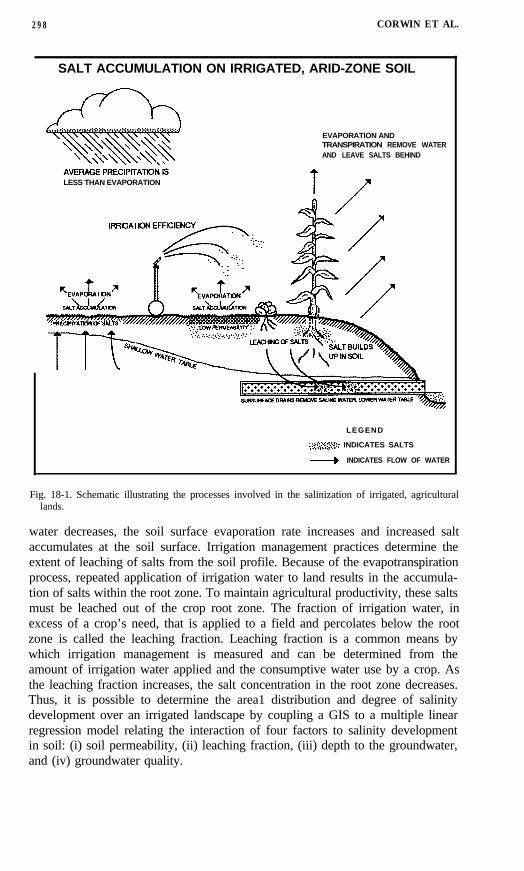
A regression model of salinity development was formulated upon com-monly known cause-and-effect salinization factors (Corwin et al., 1988, 1989;Corwin & Rhoades, 1988). In arid climates, the development of soil salinity onirrigated lands can be conceptually related to several general factors: irrigationwater quality, physical edaphology, groundwater characteristics and irrigationmanagement. Figure 18-1 illustrates the interacting dynamics of these saliniza-tion factors.

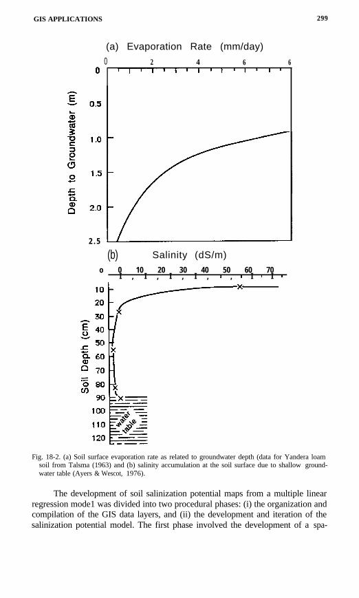
The interaction of the factors illustrated in Fig. 18-1 causes the buildup ofsalts in the root zone. Evapotranspiration, which results in the selective removalof water by plant roots leaving behind any salts naturally present in the irrigationwater, is the process primarily responsible for the accumulation of salt in the rootzone. Under steady-state conditions with a net downward water flux, salt con-centration will increase with depth through the root zone. All things being equal,irrigation water of poor quality (i.e., high salt concentration) results in higher soilsalinity profiles. Edaphic factors such as soil permeability are potentially influ-ential upon the accumulation of salt in soil due to the retarding effect upon waterflow which reduces any leaching of salts. A shallow water table and high salini-ty groundwater also are likely to be influential in the development of soil salini-ty as a result of the increased potential for upward movement of salts (Ayers &Westcot, 1976; Shih, 1983). Figure 18-2a shows the relationship between the sur-face evaporation rate and depth to the groundwater, while Fig. 18-2b shows theaccumulation of salt near the soil surface due to the upward movement of saltscarried by water rising to meet the evaporative demand. As the depth to ground-

298 CORWIN ET AL.

SALT ACCUMULATION ON IRRIGATED, ARID-ZONE SOIL

EVAPORATION ANDTRANSPIRATION REMOVE WATERAND LEAVE SALTS BEHIND

LESS THAN EVAPORATION

LEGEND

:,$$.:; INDICATES SALTS

+ INDICATES FLOW OF WATER

Fig. 18-1. Schematic illustrating the processes involved in the salinization of irrigated, agriculturallands.

water decreases, the soil surface evaporation rate increases and increased saltaccumulates at the soil surface. Irrigation management practices determine theextent of leaching of salts from the soil profile. Because of the evapotranspirationprocess, repeated application of irrigation water to land results in the accumula-tion of salts within the root zone. To maintain agricultural productivity, these saltsmust be leached out of the crop root zone. The fraction of irrigation water, inexcess of a crop’s need, that is applied to a field and percolates below the rootzone is called the leaching fraction. Leaching fraction is a common means bywhich irrigation management is measured and can be determined from theamount of irrigation water applied and the consumptive water use by a crop. Asthe leaching fraction increases, the salt concentration in the root zone decreases.Thus, it is possible to determine the area1 distribution and degree of salinitydevelopment over an irrigated landscape by coupling a GIS to a multiple linearregression model relating the interaction of four factors to salinity developmentin soil: (i) soil permeability, (ii) leaching fraction, (iii) depth to the groundwater,and (iv) groundwater quality.


2 . 5

(a) Evaporation Rate (mm/day)

0 2 4 6 6

(b) Salinity (dS/m)

o 0 10 20 30 40 50 60 70I , I , I , I , r , 1 I 1 I 1

Fig. 18-2. (a) Soil surface evaporation rate as related to groundwater depth (data for Yandera loamsoil from Talsma (1963) and (b) salinity accumulation at the soil surface due to shallow ground-water table (Ayers & Wescot, 1976).

The development of soil salinization potential maps from a multiple linearregression mode1 was divided into two procedural phases: (i) the organization andcompilation of the GIS data layers, and (ii) the development and iteration of thesalinization potential model. The first phase involved the development of a spa-

300 CORWIN ET AL.

a Broadview Irrigation District

b.- WELLTON-MOHAWK IRRIGATION DISTRICT

Fig. 18-3. (a) Location of the Wellton-Mohawk Irrigation District and the Broadview Water Districtwithin the continental USA and (b) Wellton-Mohawk Irrigation District study area showing thesection lines and the salinity traverse sample sites.

tial database of georeferenced data for a study area. The selected study site wasan area of approximately 170 square miles of the Wellton-Mohawk IrrigationDistrict located outside Yuma, AZ, in the southwestern USA (see Fig. 18-3a and18-b). The spatial database consisted of the four salinization factors: soil typewith its associated soil permeability, depth to the groundwater and groundwaterquality contour data, and leaching fraction data aggregated to Public Survey quar-ter section units. Contour maps of depth to groundwater, and groundwater quali-ty were obtained from the Wellton-Mohawk Irrigation District. Each map wasdigitized by hand and associated attributed data were entered into the GIS foreach map unit. Soil survey maps of the Wellton-Mohawk Irrigation District wereobtained from the Soil Conservation Service. Similarly, these maps were digi-tized and associated soil permeability attribute data were entered into the GIS.Finally, crop history data was obtained from the Wellton-Mohawk Irrigation Dis-trict including irrigation amounts, crops planted, and consumptive water use ofeach crop. From this data the leaching fraction was calculated for each quartersection. The quarter sections were digitized by hand and the associated leaching


DEPTH TO GROUND WATER TRENDS FOR THE

WELLTON-MOHAWK IRRIGATION DISTRICT

x LESS THAN 4 FEET

A LESS THAN 6 FEET

0 LESS THAN 8 FEET

0 0

Stable Ground Water Elevationi F 2. I---- Jan.. 1 9 6 6 - D e c . . 1 9 7 2

::ew 45- 0 O0 0 0 0l 4 O

000

10

- 0 0

0

0 0 0 0 oAA

bf 0 0 A:: E 0

fZ AA A

AA~$A@~$AA~AA~~AAA xX

s!!!Xxx

r& 0 1968 1969 1970 1971 1972 1973 1974

DATE

Fig. 18-4. Groundwater elevation trends in the Wellton-Mohawk Irrigation District from January1968 to December 1973. (1 acre = 0.405 ha; 1 foot = 0.305 m).

fraction data entered into the GIS. Though pertinent to the development of soilsalinity, irrigation water quality was ignored because it was assumed to be of uni-form quality for the entire study area. This assumption was most likely validbecause the source of the irrigation water was the same for all irrigated fields andthe quality of the water was not temporally variable. Spatial data for the foursalinization factors were compiled for the time period 1968 to 1973, a period inwhich no unusual perturbations (e.g., flooding) in the dynamics of the salinitydevelopment process for the study area had occurred as reflected by stablegroundwater elevations (see Fig. 18- 4).

The second phase involved the formulation and testing of the salinizationmodel followed by the iteration of the model to the georeferenced databank toproduce a final map. In order to formulate and validate the salinization model, asalinity traverse data set of 66 sample sites (see Fig. 18-3b for the sample sitelocations) collected by the University of Arizona in 1973 was used as the ground-truth measure of soil salinity for the top 61 cm (24 inches) of soil. The data set of66 observations was randomly split into two data sets: an estimation data set of29 observations and a validation data set of 37 observations. The estimation dataset was used to formulate a multiple linear regression model, and the validationdata set was used to evaluate the regression model. Each salinization factor wasweighted according to its significance in the overall salinization process. Theweighted significance ascribed to each factor was determined using standard sta-tistical methods (i.e., multiple linear regression) that correlate the geocoded vari-ables to the ground-truth measurements of salinity. In other words, regression

302 CORWIN ET AL.

MAP OVERLAY CONCEPT

Fig. 18-5. Schematic of map overlaying of salinization factors.

coefficients of the salinization potential model were derived by using multiplelinear regression to fit the four salinization parameters to the ground-truth soilprofile salinity measurements (meq L-l) comprising the estimation data set. Todetermine which of the four regressor variables were significant, a variable selec-tion procedure was used which would provide a large coefficient of determina-tion (R2), a small estimation of error variance (s2) and a model that is parsimo-nious. The regression model was applied to each delineated map unit generatedfrom the map overlaying capability of the GIS, specifically ARC/INFO (see Fig.18-5 for map overlay illustration). Applying the salinization potential model tothe four salinization factor databases, the GIS computed map units that were sub-sequently assigned to one of three soil salinity categories as defined in the U.S.Salinity Laboratory’s Handbook 60 (1954): low, medium, and high, correspond-ing to salt concentrations of less than 7.5 meq L-’ between 7.5 and 16.9 meq L-tand greater than 16.9 meq L-l), respectively. The maps were thereby a spatialexpression of the salinity model. To evaluate the multiple linear regressionmodel, salinities calculated from the model were compared with the measuredsalinities from the validation data set. A linear least squares analysis of the mea-sured and predicted salinities was conducted to evaluate their 1:l correspon-dence. In addition, an evaluation of the correspondence of the calculated and theobserved salinization category for each point of the validation data set was made.

Transient-State GIS/Salinity Model

The one-dimensional, functional transport model TETrans, introduced byCorwin and Waggoner (1990) and Corwin et al. (1991), was integrated into the


ARC/INFO geographic information system. TETrans was loosely coupled toARC/INFO, implying that the GIS and model software were coupled sufficient-ly to allow the transfer of data and results; consequently, the GIS and modelingmodule did not share the same data structures. A detailed discussion of the cou-pling of TETrans to the GIS is provided in Vaughan and Corwin (1995).

A complete description of the theoretical development of TETrans is out-lined in Corwin and Waggoner (1991) and Corwin et al. (1991). TETrans is amass-balance, layer-equilibrium model that defines nonvolatile, solute transportas a sequence of events or processes: (i) infiltration and drainage to field capaci-ty, (ii) instantaneous chemical equilibration for reactive solutes, (iii) water uptakeby the plant root resulting from transpiration and evaporative losses from the soilsurface, and (iv) instantaneous chemical reequilibration. Each process is assumedto occur in sequence as opposed to the collection of simultaneous processes thatactually occur in nature. Furthermore, each sequence of events or processesoccurs within each depth increment or layer of a finite collection of discrete depthincrements. The physical and chemical processes that are accounted for inTETrans include fluid flow, preferential flow, adsorption, and evapotranspirationthrough plant root water uptake. From a knowledge of water inputs and losses,and of soil-solute chemical interactions, TETrans predicts the average concentra-tion of reactive or nonreactive solutes through the vadose zone. The principaldesign philosophy behind TETrans was to develop a model around data which iscommonly collected by irrigation districts or is present in existing soil databases.This design criteria would enable the model to be applied at a regional scale inthe most cost-effective manner.

ARC/INFO was integrated with TETrans to provide spatial coverage tocompute area1 distributions of soil salinity profiles and salt-loading to the ground-water over a selected geographic area. Both the computed results and all datarequired by TETrans are stored in the GIS database to permit spatial representa-tion of any physical, chemical or biological variable.

Thirty-seven quarter sections (2396 ha) of the Broadview Water Districtlocated on the west side of central California’s San Joaquin Valley were chosenas a test site (see Figs. l8-3a and 18-6). This provided sufficient variability andmagnitude to test the methodology and the GIS/TETrans model, referred to asTETransgeo. A complete data set of spatially-referenced input parameters includ-ing irrigation data (i.e., irrigation dates, and the corresponding irrigation amountsand salt concentrations), crop data, (i.e., evapotranspiration amount between irri-gation events; maximum root penetration depth of each crop; plant water uptakedistribution of each crop; and the planting date, harvesting date and days tomaturing of each crop), soil property data (i.e., thickness and bulk density of eachsoil horizon or layer) and initial conditions (i.e., initial water content and initialsoil solution salt concentration for each soil layer) was assembled for the 1991growing season (April to September) and entered into the GIS database.

In April and May of 1991, electromagnetic induction (EM) measurementsof bulk soil electrical conductivity were taken at 64 locations (grid spacing of0.16 km) within each of the 37 quarter sections (approximately 2350 total sites)of the Broadview Water District. April and May represent the time when nearlyall of the crops in the study area were planted. From the roughly 2350 sites, a total

304 CORWIN ET AL.

Thiessen polygon coverage for Broadview Water District field area

Points are:

l measurement locations

l locations for 1-D transport m

Fig. 18-6. Boundary lines of the 37 quarter sections of the Broadview Water District test site and the285 soil sample sites. Thiessen polygons also are defined.

of 285 locations were statistically selected as representative soil sampling sitesthat represented approximately eight sample sites per quarter section (see Fig.18-6 for sample locations). The statistical selection of the 285 soil sampling siteswas based on the observed EM field pattern utilizing the technique of Lesch et al.(1992).

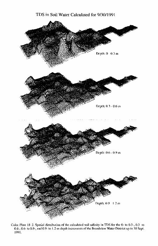
The initial conditions of water content and total salt concentration in thesoil solution were established from the soil core samples taken at 0.30-m incre-ments down to a depth of 1.2 m. A table was constructed from these measure-ments and stored in ARC/INFO format along with tables containing other rele-vant input data. Together these tables form a relational database for the Broad-view Water District. The table of initial conditions contains records for the 285locations. Each record included data for four depth increments: 0- to 0.3-, 0.3- to0.6-, 0.6- to 0.9-, and 0.9- to 1.2-m. When the TETrans program was run, the ini-tial conditions and other input data required for the calculation were obtainedfrom these tables.

The boundary condition at the surface was established by the irrigationschedule for each quarter section. Irrigations generally occurred during a 2- to 3-day period. There were normally four to seven such periods during the summergrowing season. The TETrans calculation requires that irrigation be characterizedas specific events in which an amount of water is applied instanteously; therefore,the actual stored data representing the boundary conditions consists of irrigationevent records containing the depth of water applied, the date applied, and the saltconcentration of the irrigation water. The TDS (total dissolved solids) for eachirrigation water was estimated from the electrical conductivity. Chemical analy-ses of the irrigation water were performed by the Soil Testing Laboratory at Col-orado State University. Sampling was conducted at approximately 1-mo intervals.

GIS APPLICATIONS 30.5

The evapotranspiration (ET) was determined for each crop with CIMIS (Califor-nia Irrigation Management Information System) data for the vicinity of theBroadview Water District.

Thiessen polygons were created from the 285 sample sites (see Fig. 18-6).The TETrans model was applied for each of the map units defined by theThiessen polygons. Results of the TETrans simulations are presented for the maingrowing season of 1991. Preliminary display maps show calculated area1 distrib-utions of irrigation efficiency (i.e., leaching fraction), drainage amounts and salt-loading to groundwater for the time period from April, 1991, to September 30,1991. Future simulations will be conducted up to the project’s expected termina-tion date of 1996. In 1996 field measurements of salinity at the 285 locations willbe measured for comparison with simulated results from the GIS/TETrans model.

RESULTS

Steady-State GE/Salinity Model

The best regression model of salinity development both in its goodness-of-fit to the estimation data set and in its ability to reliably predict the salinities ofthe validation data set consisted of three significant regressor variables: soil per-meability (cm h-t), leaching fraction and groundwater electrical conductivity (dSm-t). As shown below, the functional form of the model indicated that the salin-ity (in meq L-t) in the top 61 cm of the soil was inversely related to the soil per-meability and the leaching fraction, and directly related to the electrical conduc-tivity of the groundwater. The depth to the groundwater was determined to be aninsignificant parameter due to the lack of a shallow water table:

SALINITY (meq L-‘) = 18.03 x (l/permeability) - 0.40

x (l/leaching fraction) + 1.32

x (groundwater electrical conductivity) + 2.12 [1]

The R2 for Eq. [l] was 0.86 showing a fairly high degree of fit. The estimator oferror variance, s*, was comparatively low, 2.59. Because the leaching fractionwas not available for all quarter sections, a second regression equation (Eq. [2])also was formulated. When leaching fraction data was not available, the perme-ability and groundwater electrical conductivity were the significant regressorvariables formulating the model:

SALINITY (meq L-t) = 23.16 x (l/permeability)

+ 0.84 (groundwater electrical conductivity) + 1.26 [2]

The R2 and s2 for Eq. [2] were 0.60 and 10.64, respectively. The significantdecrease in the R2 and the increase in the s2 when leaching fraction was removedas a regressor variable indicated that leaching fraction was particularly significantin the model.

306 CORWIN ET AL.

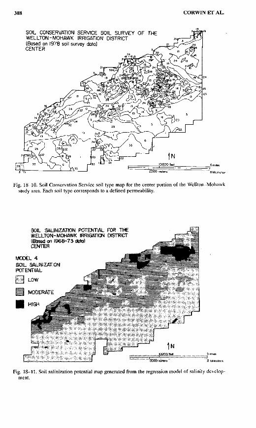
LEACHING FRACTION FOR EACH QUARTER SWITHIN THE WELLTON-MOHAWK IRRIGATION(Based on 1970-72 data)CENTER

Fig. 18-7. Leaching fraction for each quarter section of the center portion of the Wellton-Mohawkstudy area.

Figures 18-7 to 18-10 show the spatial representation of the four saliniza-tion factors. For visualization detail purposes only the center portion of the Well-ton-Mohawk is shown. The map of salinization potentials generated from theregression model (see Fig. 18-11) indicated general trends in salinity that wereknown to exist for the study area over the time period of interest, 1968 to 1973.The southern half of the irrigation district is a mesa on which low salinity exist-ed. Generally speaking, the northern half was predominantly moderate in salini-ty with pockets of low and high salinities.

The ability of the model to correctly predict both the salinity category (low,medium, and high) and the actual measured soil salinity value was very good. Outof the 37 observations in the validation data set, the model was able to predict86% of the categories correctly. Even more impressive was the close predictionof actual measured salinity values in the validation data set. A linear regressionof predicted salinity values from the model and measured salinities resulted in aslope andy-intercept of 1.000 and -0.001, respectively, with an R2 of 0.81. A plotof the residuals for the model showed an ideal residual plot with a random pat-tern around zero and no detectable trend. This fact further established the finalformulation of the model as the most reliable.


Simulated results for the top 1.2 m of soil calculated for the time period ofApril 1991 to 30 September 1991, show the most significant change in salinityoccurs in the top 0.3 m of the soil profile (compare Color Plates 18-l and 18-2).Noticeable salinity concentration increases occurred in the top 0.3 m at several


locations (see Color Plate 18-2). In every instance the salinity peaks are locatedon soil that had been left fallow. The peaks are most likely artifacts of theTETrans model and they point out one of the inherent weaknesses of the TETransmodel. TETrans does not account for the upward movement of water; conse-quently, TETrans does not replenish the depleted water of the surface layer withmoisture from lower in the profile. Without a calculation for upward water flow,the continuous removal of water by surface evaporation on fallow fields resultsin the depletion of water in the 0- to 0.3-m depth increment down to the residualwater content (i.e., approximately the water content of air dried soil). The resul-tant calculated concentration of salts within the top layer is raised to an extreme-ly high level. Even though the calculated upward movement of moisture to meetevaporative demand also would bring salt, it would not bring enough salt toapproach the level of salinity calculated from the depletion of moisture in the toplayer down to the residual water content; consequently, the salinity level calcu-lated by TETrans for the surface layer of fallow areas is spuriously high.

Color Plate 38-3 shows the calculated leaching fractions for the prelimi-nary 6-mo study period. An area totaling approximately twelve quarter sectionshad a calculated leaching fraction of less than 0.1. This area consisted of eitherfallow land or land which had a crop of seed alfalfa (see Color Plate 18-4). Theapplication and/or precipitation of water in these areas totaled less than 0.1 m.The spatial distribution of the calculated amount of drainage beyond the root zoneis shown in Color Plate 18-5. A composite area equal to greater than seventeenquarter sections had a drainage of less than 0.1 m.

Color Plate 18-6 shows an area1 distribution of the amount of salt thatdrained beyond the root zone and will ultimately enter the groundwater. Most ofthe study area shows very little salt loading because a significant portion of theland was fallow (no irrigation water was applied) for the preliminary 6-mo studyperiod resulting in little drainage. Because little rainfall occurred in 1991, the fal-low areas had no net calculated downward salt flux. In fact, evaporation exceed-ed rainfall during this time period. The greatest salt loading to the groundwateroccurred in Section 3SE (i.e., the southeast quarter section of Section 3), Section4NE, Section 8SE, and Section 15NE (see Color Plate 18-6). Not surprisingly,these areas are associated with high leaching fractions (i.e., in most cases leach-ing fractions ranging from 0.4 to 0.8; see Color Plate 18-3), and high soil salini-ty in the lower portion of the soil profile (see Color Plate 18-1, depths 0.6-0.9 mand 0.9-1.2 m). All four quarter sections were cropped with cotton (Gossypiumhirsutum L.). An inventory of the extent of salt-affected soils for the BroadviewWater District is shown in Color Plate l8-7.

DISCUSSION OF RESULTS AND CONCLUSIONS

Steady-State GE/Salinity Model

The regression model indicated by the magnitude of its coefficients thatelectrical conductivity of the groundwater and soil permeability were the domi-nating soil salinization factors in the Wellton-Mohawk Irrigation District over theperiod of study. Leaching fraction had only subtle effects. In spite of this fact, themodel also showed that the greatest single increase in R2 for a multivariate case

310 CORWIN ET AL.

occurred for the combination of leaching fraction and electrical conductivity ofthe groundwater. This suggests that salinity development within the soil profilewas more a consequence of the leaching fraction with the groundwater electricalconductivity merely acting as a reflection of the leaching efficiency and the elec-trical conductivity of the irrigation water. Several other facts point to leachingfraction as the predominant mechanism of salinity development in this particularstudy. First, the correlation matrix for the model indicated an inverse correlation-ship (I = -0.71) between groundwater electrical conductivity and leaching frac-tion. The moderate negative correlation combined with the negative sign and theinsignificant magnitude of the leaching fraction coefficient in Eq. [l] suggests theexistence of multicollinearity. Second, depth to the groundwater was insignificantto the development of soil salinity. This was shown by the statistical insignifi-cance of depth to groundwater as a regressor variable in the formulation of theregression model with the variable selection procedure. Figures 18-2 and 18-8provide reaffirmation of this contention. Figure 18-8 shows that very few loca-tions have a water table shallower than 1.5 m (5 ft); consequently, the influenceof the depth to groundwater may not come into play. The evaporation rate at thesoil surface, which is the driving force behind upward water flow on bare sur-faces, quickly diminishes as the depth to groundwater exceeds 1.5 m (see Fig.18-2). This would make the broad scale upward movement of salinity an unlike-ly mechanism for salinization in this study area. Third, leaching fraction was neg-atively correlated to soil salinity as would be expected if irrigation managementwas the dominating mechanism influencing soil salinity development. Thoughthe results are inconclusive, the model points to irrigation management as theoverall predominant mechanism for determining the development of salinity inthe root zone for the study area and the time period of interest. Ostensibly, thehigh correlation of groundwater electrical conductivity to soil salinity develop-ment is actually a reflection of the irrigation efficiency and irrigation water salin-ity.

The obvious limitations to the use of regression models for characterizingsoil salinity development or for quantifying any natural process for that matterare: (i) site specificity and (ii) most probably time specificity. Different locationswill undoubtedly have different predominant mechanisms. Furthermore, any per-turbations to cause the system to no longer be at steady state immediately negatesthe continued application of the model.

This approach has extremely limited application. Nevertheless, as long assteady state conditions remain in effect with the same mechanisms predominat-ing, and as long as the inputs into the regression model are not outside the rangeof the estimation data set, then reliable predictions are possible. If nothing else,this approach provides a visualization of the area1 distribution of potential salin-ity development for inventory purposes which surpasses the spatial informationprovided by a map of point soil salinity measurements.


The justification for the role of the GIS in manipulating and displaying spa-tial data is profoundly revealed in the simulations presented in Color Plates 18-2,


18-3, 18-5, 18-6, and 18-7. These figures are the result of input data spatiallydefined by Thiessen polygons created around soil-core sample sites; quarter sec-tions which defined irrigation map units and crop map units (i.e., evapotranspira-tion units); and a chloropleth map which defined soil types with their associatedphysical and chemcial properties. From the layers of geometrically-diverse geo-referenced information the GIS permitted the display of simulated results as poly-gons (Color Plates 18-3, 18-5, 18-6, and 18-7) or as interpolated three-dimen-sional visualizations (Color Plate 18-2).

Quarter Sections 3SE, 4NE, 8SE, and 15NE (see Fig. 18-6) have highleaching fractions (see Color Plate l8-3), high drainages (see Color Plate l8-5),and high salt leaving the root zone (see Color Plate 18-6). Because these quartersections were cropped with cotton (see Color Plate 18-4), which is a highly salt-tolerant crop, it is obvious that the salt-load could have been reduced by applyingless irrigation water during the 6-mo preliminary study period. Irrigation amountsfor Quarter Sections 3SE, 4NE, 8SE, and 15NE were OS-O.6 m, 0.3-0.4 m,0.4-0.5 m, and 0.4-0.5 m, respectively. Reduced irrigation amounts would nothave adversely affected crop production. A close look at the initial (April andMay, 1991) and the simulated soil salinity profiles (30 Sept. 1991) for these quar-ter sections reveals that most of the salt that moved beyond the root zone camefrom the lower portion of the root zone (0.6-1.2 m). Even at a reduced irrigationapplication, the low initial salinity in the upper portion of the soil profile (O-0.6m) at the time of planting would have permitted germination and maturation ofthe cotton. Though different factors may be responsible for the cause of the salt-loading, it becomes readily apparent from the displayed spatial information ofsalinity distributions how to manage various situations.

Color Plate 18-7 provides a useful inventory of salt-affected soil. If depth-averaged soil salinity for the top 1.2 m can be used as a measure of salt-affectedsoil, then approximately 40% of the 2400-ha study area would be defined assaline. An inventory of salt-affected soils is of value in assessing the extent of theimpact of agricultural activities upon soil. Knowing the extent of the problem isthe first step in determining whether or not there is a problem, and whether theproblem is getting better or worse.

SUMMARY

The ability to show area1 distributions of soil salinity over time provides anessential tool for maintaining a sustainable agriculture by supplying the informa-tion needed to optimize food production while minimizing the use of finite nat-ural resources such as water, and minimizing impacts upon the environment. Twodifferent GIS-based approaches for assessing the impact of a non-point sourcepollutant (i.e., soil salinity) on soil and groundwater resources of agriculturallands have been presented that can be used under different conditions (i.e., steadystate or transient state).

The ability to predict salt accumulation in soil from soil features and tovisually display their area1 distribution provides an invaluable tool for agricultur-al management purposes. It can serve as a means of locating salinity monitoring

312 CORWIN ET AL.

sites, to assist in formulating irrigation management practices, and to select crops.Area1 distributions of salt accumulation in the root zone indicate areas whereclose attention to crop selection and irrigation management should be paid tomaximize crop yield. Soil salinization potential maps can serve as a guide fordetermining reclamation needs, or for deciding if cultivated lands should bebrought into production or left untouched. Finally, an assessment of soil salinitycan be made without labor-intensive field measurements of salinity by invento-rying the extent of salt-affected soils as predicted from soil property relationships.

To minimize the environmental impact of salinity upon groundwaterresources, a spatial knowledge of leaching efficiency and salt-loading is neces-sary. Area1 distributions of salt-loading to the groundwater define areas where thegreatest attention must be given to reduce the downward flux of salt eitherthrough changes in irrigation management strategy or installation of drainage sys-tems.

ACKNOWLEDGMENTS

The authors wish to thank the American Society of Agricultural Engineersfor their permission to reproduce Color Plates l8-l, 18-2, and 18-6; and to thankElsevier Science Publishers for their permission to reproduce Figs. 18-3b, 18-4,18-7, 18-8, 18-9, 18-10, and 18-11.

REFERENCES

Ayers, R.S., and D.W. Wescot. 1976. Water quality for agriculture. Food and Agric. Organ. of theU.N., Irrig. and Drainage Pap. 29. FAO, Rome.

Corwin, D.L. 1996. GIS applications of deterministic solute transport models for regional-scaleassessment of non-point source pollutants in the vadose zone. p. 69-100. In D.L. Corwin andK. Loague (ed.) Applications of GIS to the modeling of non-point source pollutants in thevadose zone. SSSA Spec. Publ. 48. SSSA, Madison, WI.

Corwin, D.L., and J.D. Rhoades. 1988. The use of computer-assisted mapping techniques to delineatepotential areas of salinity development in soils: II. Field verification of the threshold modelapproach. Hilgardia 56(2):18-32.

Corwin, D.L., M. Sorensen, and J.D. Rhoades. 1989. Field-testing of models which identify soils sus-ceptible to salinity development. Geoderma 45:31-64.

Corwin, D.L., P.J. Vaughan, H. Wang, J.D. Rhoades, and D.G. Cone. 1993a. Coupling a solute trans-port model to a GIS to predict solute loading to the groundwater for a non-point source pol-lutant. p. 485-492. In C.D. Heatwole (ed.) Proc. of the ASAE Application of Advanced Infor-mation Technologies: Effective Management of Natural Resources, Spokane, WA. 18-19 June1993. Am. Soc. of Agric. Eng., St. Joseph, MI.

Corwin, D.L., P.J. Vaughan, H. Wang, J.D. Rhoades, and D.G. Cone. 1993b. Predicting areal distrib-utions of salt-loading to the groundwater. In Int. Winter Meeting of the Am. Soc. of Agric.Eng., Chicago, IL. 14-17 Dec. 1993. Pap. 932566. Am. Soc. of Agric. Eng., St. Joseph, MI

Corwin, D.L. , and B.L. Waggoner. 1990. TETrans: A user-friendly, functional model of solute trans-port. J. Water Sci. Technol. 24(6):57-66.

Corwin, D.L., and B.L. Waggoner. 1991. TETrans: Solute transport modeling software user’s guide$,M,““trh and IBM versions). U.S. Salinity Lab. Publ. 121 and 123. USDA-ARS Washing-

Corwin, D.L., B.L. Waggoner and J.D. Rhoades. 1991. A functional model of solute transport thataccounts for bvpass. J. Environ. Qual. 20:647-658.

Corwin, D.L., J.W. Werle, and J.D. Rhoades. 1988. The use of computer-assisted mapping techniquesto delineate potential areas of salinity development in soils: I. A conceptual introduction. Hil-gardia 56(2):1-17.


Hopkins, R.B., Jr., and J.C. Clausen. 1985. Land use monitoring and assessment for nonpoint sourcepollution control. p. 25-29. In Perspective on nonpoint source pollution. U.S. Environ. Pro-tection Agency, Kansas City, MO.

Lesch, SM., J.D.Rhoades, L.J. Lund and D.L. Corwin. 1992. Mapping soil salinity using calibratedelectromagnetic measurements. Soil Sci. Soc. Am. J. 56(2):540-548.

Pelletier, R.E. 1985. Evaluating nonpoint pollution using remotely sensed data in soil erosion models.J. Soil Water Conserv. 40(4):332-335.

Potter, W.B., M.W. Gilliland, and M.D. Long. 1986. A geographic information system for predictionof runoff and non-point source pollution potential. p. 437-446. In A.I. Johnson (ed.) Hydro-logic applications of space technology. Int. Assoc. Hydrologic Sci. Publ. 160. Int. Assoc.Hydrologic Sci., IAHS Press, Wallingford, Oxfordshire, England.

Shih, S.F. 1983. Soil surface evaporation and water table depths. J. Irrig. Drain. Eng. 109(4):366-374.Talsma, T. 1963. Meded. Landb. Hoogesch. Wageningen. 63(10):1.U.S. Salinity Laboratory. 1954. Diagnosis and improvement of saline and alkali soils. Agric. Handb.

60. USDA, Washington, DC.Vaughan, P.J., D.L. Corwin, and H. Wang. 1993. Coupling a chemical transport model to a GIS data-

base for assessment of non-point source pollution in irrigated agricultural areas. p. 127-138.In Proc. of the 13th Annual ESRI User’s Conf., Palms Springs, CA. 24-28 May 1993. Envi-ron. Syst. Res. Inst., Redlands, CA.

Vaughan, P.J., and D.L. Corwin. 1995. A method of modeling vertical fluid and solute transport in aGIS context. Geoderma 64(1-2):139-154.

18 gis applications to the basin-scale assessment of soil salinity

Documents