16 Analysis of Water Balances N.A. de Ridder'? and J. Boonstra'

16.1 Introduction

Analyses of water balances are necessary to calculate an area's drainable surplus (drainage requirement), which we define here as the quantity of water that flows into the groundwater reservoir in excess of the quantity that flows out under natural conditions. Removing the drainable surplus has two advantages: it prevents waterlogging by artificially maintaining a sufficiently deep watertable and it removes enough water from the root zone so that any salts brought in by irrigation cannot reach a concentration that would be harmful to crops.

Calculating the drainable surplus is a major problem in many irrigation and reclamation areas. The natural conditions in these areas are diverse, and different water resources may be involved in the calculations. It is therefore necessary to do field work on the general features of the groundwater regime and to study the water and salt regimes and their balances. A proper understanding of these regimes allows the drainage engineer to predict how they will be affected by drainage and reclamation works.

The factors involved in calculating the drainable surplus are derived from analysis of the overall water balance of the study area. The balance method, however, can be used only if it is possible to determine directly all components of the water and salt balance with sufficient accuracy. If the results of several independent balance analyses do not agree, the drainage engineer can compare the degree of discrepancy to get an idea of the reliability of the obtained data and to see if further observation and verification are necessary.

This chapter starts with a description of the different elements of water balance equations and goes on to discuss the water balance of the unsaturated zone, the surface water balance, the groundwater balance, and the integrated water balance. Salt balances are discussed briefly in a subsequent section. (See Chapter 15 for a more detailed treatment of salt balances in the root zone in irrigated soils.) A brief explanation of numerical groundwater models is included in Section 16.4. The chapter concludes with a few examples of water balance analysis.

16.2 Equations for Water Balances

The water balance is defined by the general hydrologic equation, which is basically a statement of the law of conservation of mass as applied to the hydrologic cycle. In its simplest form, this equation reads

(16.1)

Water balance equations can be assessed for any area and for any period of time.

Inflow = Outflow + Change in Storage

' International Institute for Land Reclamation and Improvement

60 1

It is worth noting that the word ‘area’ is commonly used in the professional jargon to mean ‘volume’, i.e. a certain part of a three-dimensional flow domain. The process of ‘making an overall water balance for a certain area’ thus implies that an evaluation is necessary of all inflow, outflow, and water storage components of the flow domain as bounded by the land surface, by the impermeable base of the underlying groundwater reservoir, and by the imaginary vertical planes of the area’s boundaries.

The water balance method has four characteristic features. They are: - A water balance can be assessed for any subsystem of the hydrologic cycle, for any

size of area, and for any period of time; - A water balance can serve to check whether all flow and storage components

involved have been considered quantitatively; - A water balance can serve to calculate the one unknown of the balance equation,

provided that the other components are known with sufficient accuracy; - A water balance can be regarded as a model of the complete hydrologic process

under study, which means it can be used to predict what effect the changes imposed on certain components will have on the other components of the system or subsystem.

16.2.1 Components of Water Balances

Time Water balances are often assessed for an average year. But waterlogging and salinity problems are not of the same duration or frequency throughout the world. In some regions, they are permanent (e.g. in marshy areas, which are topographic depressions with a permanently high watertable caused by a combination of surface and subsurface inflow). In others, they are temporary (e.g. in areas of incidentally high rainfall or in irrigation areas that receive large quantities of surface water only during the irrigation season). In both cases, the watertable rises to an unacceptable level because the natural drainage of the area cannot cope with the excessive recharge of the groundwater reservoir.

If the watertable remains high for long periods, crop yields will diminish. In areas where waterlogging occurs, it is necessary to assess water balances not only for an average year, but also for specific years and even for specific seasons (e.g. the growing season, the irrigation season, or, in irrigation areas in arid and semi-arid climates, the period of leaching the soil to prevent salinization).

Flow Domain Let us say that we want to make a water balance study of a certain surface area. We can choose from two types of flow domains. They are: - Flow domains comprising physical entities (e.g. river catchments and groundwater

- Flow domains comprising only parts of physical entities (e.g. irrigation schemes basins);

and areas with shallow watertables).

Let us assess the water balance of the river catchment shown in Figure 16.1. Suppose

602

,_--_

PLAN

__.-- _-- catchment boundary /.-- --...__

-._*___--- i and water divide.,

outlet

I \

Figure 16.1 River catchment with a single outlet in bedrock

that field work has shown that the boundary of the catchment coincides with the groundwater divide. The divide can be regarded as an impermeable boundary because no groundwater flows across it.

Let us assume that the area lies in a humid climate, where changes in water storage usually follow an annual cycle. By choosing dates that are one year apart when we decide the beginning and the end of the period for which the water balance is to be assessed, we can usually ignore the change in water storage. Rainfall is measured at several meteorological stations in the catchment. The runoff from the area is measured at the outlet. Because impermeable bedrock comes close to the land surface at the outlet, preventing groundwater outflow, all water from the catchment area leaves the area as stream flow. The overall water balance equation for the area then reads

Rainfall - River Outflow = Evapotranspiration (16.2) From this equation we can solve the unknown evapotranspiration. Dalton (1 802) was among the first to use a catchment water-balance method to correlate the measured rainfall and streamflow data with the estimated evaporation data for England and Wales, as reported by Dooge (1984). It should be noted that Equation 16.2 is a strongly simplified version of the general water balance equation presented in Section 2.5.

Artificially determined areas such as irrigation areas and areas in need of drainage usually cover only part of a river catchment or groundwater basin. Therefore, it is

603

necessary to account for surface and subsurface inflow and outflow across the vertical planes of the boundaries of these areas. If we determine all their inflow, outflow, and water storage components, we can assess the overall water balance. This is how water balance studies for subsurface drainage are usually done.

In overall water balances, we consider the flow domain vertically - from the soil surface to the impermeable base of the groundwater reservoir. The impermeable base may consist of massive hard rock or of a clay layer whose permeability for vertical flow is so low that it can be regarded as impermeable. (These are the aquicludes mentioned in Chapter 2.) Three reservoirs occur in this flow domain: at the surface itself, in the zone between the surface and the watertable, and in the zone between the watertable and the impermeable base. Because the reservoirs are hydraulically connected, it is often necessary to assess partial water balances for each of them in order to specify the drainable surplus. These water balances are referred to here as the surface water balance, the water balance of the unsaturated zone, and the groundwater balance. We shall discuss them in more detail in the sections that follow.

It is important to note that, at certain depths, there can be clay layers that behave more like aquitards than like aquicludes. The occurrence of these aquitards implies the presence of one or more confined aquifers underneath. In principle, then, it is possible to consider either a multiple aquifer system as a whole or the shallow aquifer alone. In water balance studies for subsurface drainage, it is common to consider only the shallow aquifer. This approach makes it necessary to consider the possible interaction between the deeper, confined water and the shallow, unconfined water.

16.2.2 Water Balance of the Unsaturated Zone

For any drainage study, it is absolutely essential to understand the water regime in the unsaturated zone, which extends from the land surface to the watertable. It is in this zone that favourable conditions for crop growth must be created.

Some components of a water-balance study of the unsaturated zone are (Chapter 11): - Determine the soil-water storage; - Assess the soil-water balance and define the relation between it, the water balance

of the underlying saturated zone (zone below the watertable), and the hydrometeorlogical factors;

- Assess the infiltration, evaporation and evapotranspiration, seepage and percolation, and groundwater movement (Chapters 4,5, and 9).

Clearly, for large areas, the time and money necessary to conduct such a study would be prohibitive. It would be better to do the research on balance plots or in a pilot area whose soil and hydrology are representative of conditions in the surrounding area.

The unsaturated zone consists of pores that are filled partially with water and partially with air. It can be referred to sometimes as the aeration zone or the vadose zone (a term derived from the Latin word vadosus, meaning ‘shallow’). The name ‘unsaturated’ can be misleading because there are portions of the zone that may actually be saturated even though the pressure of the water is below atmospheric

604

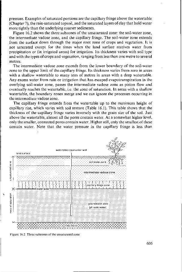
pressure. Examples of saturated portions are the capillary fringe above the watertable (Chapter 7), the rain-saturated topsoil, and the saturated layers of clay that hold water more tightly than the underlying coarser sediments.

Figure 16.2 shows the three subzones of the unsaturated zone: the soil-water zone, the intermediate vadose zone, and the capillary fringe. The soil-water zone extends from the surface down through the major root zone of crops and vegetation. I t is not saturated except for the times when the land surface receives water from precipitation or (in irrigated areas) for irrigation. Its thickness varies with soil type and with the types of crops and vegetation, ranging from less than one metre to several metres.

The intermediate vadose zone extends from the lower boundary of the soil-water zone to the upper limit of the,capillary fringe. Its thickness varies from zero in areas with a shallow watertable to many tens of metres in areas with a deep watertable. Any excess water from rain or irrigation that has escaped evapotranspiration in the overlying soil-water zone, passes the intermediate vadose zone as piston flow and eventually reaches the watertable, i.e. the zone of saturation. In areas with a shallow watertable, the boundary zones merge and we can ignore the processes occurring in the intermediate vadose zone.

The capillary fringe extends from the watertable up to the maximum height of capillary rise, which varies with soil texture (Table 16.1). This table shows that the thickness of the capillary fringe varies inversely with the grain size of the soil. Just above the watertable, almost all the pores contain water. At a somewhat higher level, only the smaller, connected pores contain water. Higher still, only the smallest of these contain water. Note that the water pressure in the capillary fringe is less than

land surface watertable observation well

I I

.intermediate vadosezone: . : 1 . : . . . . . . . . . . . . . . . . . . . . . . . . . . . . . . . . . . . . . . . . . . . . . . . . . . . . . . . . . . . . . . . . . . . . . . . . . . . . . . . . . . . . . . . :I 1: . : . . . . . . . . . . . . . . . . . . . . . . . . . . . . . . . . . . . . . . . . . . . . . . . . . . . . . . . . . . . . . . . . . . . . . . . . . . . . . . . . . . . . . . . . . . . . . . . . . . . . . . . . . . . . . . . . . . . . .

Figure 16.2 Three subzones ofthe unsaturated zone

605

Table 16.1 Capillary rise in different soils (after Lohman 1972)

Soil type Grain size Capillary rise mm mm

Fine gravel 2 - 5 25 Very coarse sand 1 - 2 65 Coarse sand 0.5 - 1 135 Medium sand 0.2 - 0.5 246 Fine sand 0.1 - 0.2 428 Very fine sand 0.005 - 0.1 1055 Coarse silt 0.002 - 0.005 > 2000

atmospheric, which means that water from this zone will not flow into a well, drain, or open borehole.

In areas with a shallow watertable, the capillary fringe may extend into the root zone of the crops and vegetation. A vertical flux from the saturated zone may then develop and move up into the unsaturated zone, from where it is removed by evapotranspiration. The rate of capillary rise, and the subsequent evaporation at the surface, decrease as the depth of the watertable increases.

Infiltrating rain and irrigation water increase the soil-water content and can cause the watertable to rise. The time required for the infiltrating water to reach the watertable increases in proportion to the depth of the watertable. Clearly then, if we want to assess the water balance of the unsaturated zone, we must consider all waters that infiltrate into it due to precipitation, irrigation, and seepage. We must know not only the maximum water-holding capacity of the soil, but also the amount of moisture stored in the zone, the actual rate of evapotranspiration of the crops, the percolation to the groundwater, and the rate of capillary rise from the groundwater. The water balance of the unsaturated zone reads

(1 6.3)

where I E G R AWu = the change in soil water storage in the unsaturated zone during the

At

= the rate of infiltration into the unsaturated zone (mm/d) = the rate of evapotranspiration from the unsaturated zone (mm/d) = the rate of capillary rise from the saturated zone (mm/d) = the rate of percolation to the saturated zone (mm/d)

computation interval of an equivalent layer of water (mm) = the computation interval of time (d)

The common assumption is that the flow direction in the zone is mainly vertical, so no lateral flow components occur in the water balance.

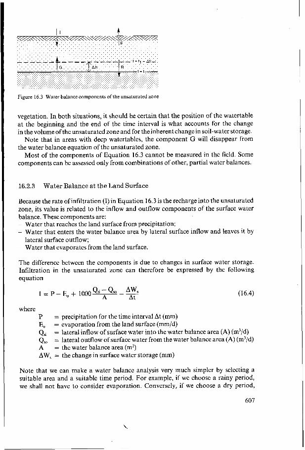
In Figure 16.3, a rise in the watertable Ah (due to downward flow from, say, infiltrating rainwater) is depicted during the time interval At. Conversely, during a period of drought, we can expect a decline in the watertable due to upward flow from capillary rise and to subsequent evapotranspiration by the crops and natural

606

. . . . . . . . . . . . . . . . . . . . . . . . . . . . . . . . . . . . . . . . . . . . . . . . . . . . . . . . . . . . . . . . . . . . . . .

where P E, Qsi

A AWs = the change in surface water storage (mm)

= precipitation for the time interval At (mm) = evaporation from the land surface (mm/d) = lateral inflow of surface water into the water balance area (A) (m3/d)

= the water balance area (m') I Q,, = lateral outflow of surface water from the water balance area (A) (m3/d)

. . . . . . . . . . . . . . . . . . . . . . . . . . .

~ Note that we can make a water balance analysis very much simpler by selecting a suitable area and a suitable time period. For example, if we choose a rainy period, we shall not have to consider evaporation. Conversely, if we choose a dry period, 1

. . . . . . . . . . . . . . . . . . . . . . . . . . . . . . . . . . . . . . . . . . . . ~ , : , ; , . . . . . . . . . . . . . . . . . . . . . . . . . . . . . . . . . . . . . . . . . . . . . . . . . . . . . . . . . . . . . . . . . . . . . . . . - - - -._ - -. -.- - - -.- A I- A' t = I r + Al I

I 607

Figure 16.3 Water balance components of the unsaturated zone

vegetation. In both situations, it should be certain that the position of the watertable at the beginning and the end of the time interval is what accounts for the change in the volume of the unsaturated zone and for the inherent change in soil-water storage.

Note that in areas with deep watertables, the component G will disappear from the water balance equation of the unsaturated zone.

Most of the components of Equation 16.3 cannot be measured in the field. Some components can be assessed only from combinations of other, partial water balances.

16.2.3 Water Balance at the Land Surface

Because the rate of infiltration (I) in Equation 16.3 is the recharge into the unsaturated zone, its value is related to the inflow and outflow components of the surface water balance. These components are: - Water that reaches the land surface from precipitation; - Water that enters the water balance area by lateral surface inflow and leaves it by

- Water that evaporates from the land surface. lateral surface outflow;

The difference between the components is due to changes in surface water storage. Infiltration in the unsaturated zone can therefore be expressed by the following equation

Qsi - Qso AWs At I = P-E, + 1000 A (16.4)

precipitation can be eliminated. We can select an area without any inflow and outflow of surface water, or we can select a time period that has the same surface water storage at the beginning and end.

In irrigated areas, the major input and output of a water balance are usually determined by two artificial components, namely the application of water for irrigation and (in arid zones) for leaching the soil, and the removal of excess irrigation water (surface drainage) and excess groundwater (subsurface drainage).

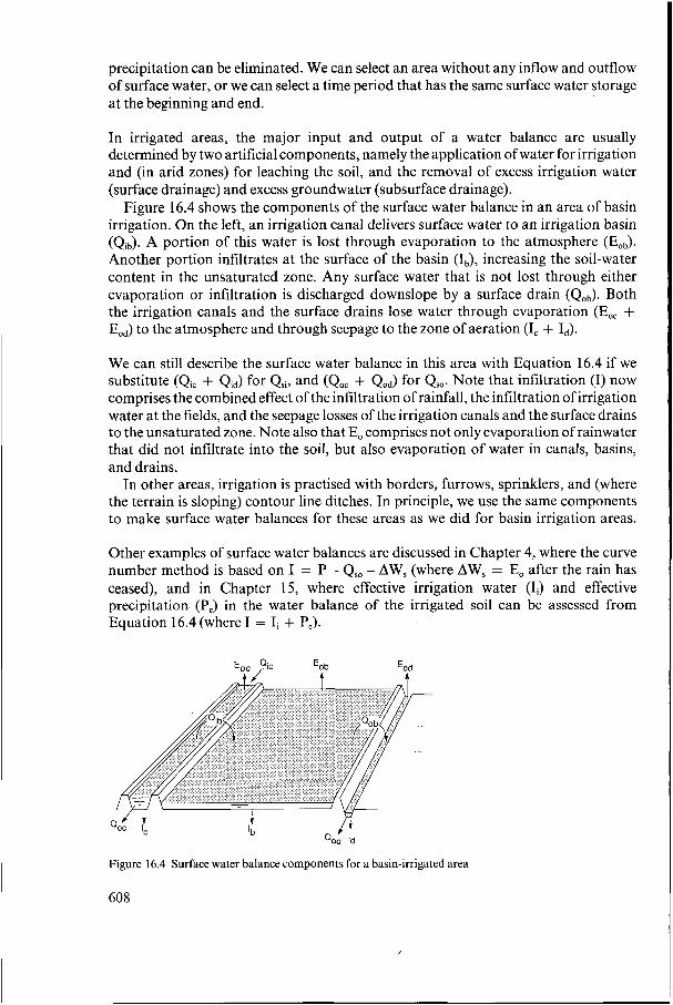
Figure 16.4 shows the components of the surface water balance in an area of basin irrigation. On the left, an irrigation canal delivers surface water to an irrigation basin (Qib). A portion of this water is lost through evaporation to the atmosphere (Eob). Another portion infiltrates at the surface of the basin (Ib), increasing the soil-water content in the unsaturated zone. Any surface water that is not lost through either evaporation or infiltration is discharged downslope by a surface drain (Qob). Both the irrigation canals and the surface drains lose water through evaporation (Eoc + Eod) to the atmosphere and through seepage to the zone of aeration (I, + Id).

We can still describe the surface water balance in this area with Equation 16.4 if we substitute (Qic + Qid) for Qsi, and (Qoc + Qod) for Q,,. Note that infiltration (I) now comprises the combined effect of the infiltration of rainfall, the infiltration of irrigation water at the fields, and the seepage losses of the irrigation canals and the surface drains to the unsaturated zone. Note also that E, comprises not only evaporation of rainwater that did not infiltrate into the soil, but also evaporation of water in canals, basins, and drains.

In other areas, irrigation is practised with borders, furrows, sprinklers, and (where the terrain is sloping) contour line ditches. In principle, we use the same components to make surface water balances for these areas as we did for basin irrigation areas.

Other examples of surface water balances are discussed in Chapter 4, where the curve number method is based on I = P - Q,, - AWs (where AW, = E, after the rain has ceased), and in Chapter 15, where effective irrigation water (Ii) and effective precipitation (P,) in the water balance of the irrigated soil can be assessed from Equation 16.4 (where I = I, + P,).

i Qoc IC 'b f l

QOd 'd

Figure 16.4 Surface water balance components for a basin-irrigated area

608

16.2.4 Groundwater Balance

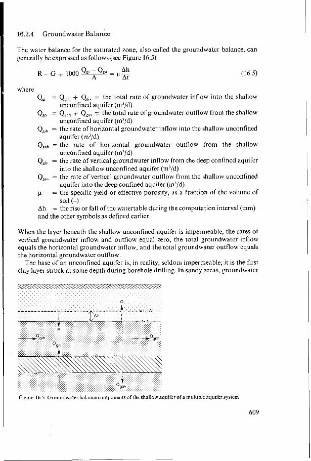
The water balance for the saturated zone, also called the groundwater balance, can generally be expressed as follows (see Figure 16.5)

Q i - Q g o - Ah - P Ä t R - G + 1000 A (1 6.5)

where Qgi = Qgih + Qgiv = the total rate of groundwater inflow into the shallow

Qgo = Qgoh + Qgov = the total rate of groundwater outflow from the shallow

Qgih = the rate of horizontal groundwater inflow into the shallow unconfined

Qgoh = the rate of horizontal groundwater outflow from the shallow

Qgiv = the rate of vertical groundwater inflow from the deep confined aquifer

Qgov = the rate of vertical groundwater outflow from the shallow unconfined

I.( = the specific yield or effective porosity, as a fraction of the volume of

Ah = the rise or fall of the watertable during the computation interval (mm) and the other symbols as defined earlier.

unconfined aquifer (m3/d)

unconfined aquifer (m3/d)

aquifer (m3/d)

unconfined aquifer (m3/d)

into the shallow unconfined aquifer (m3/d)

aquifer into the deep confined aquifer (m3/d)

soil (-)

When the layer beneath the shallow unconfined aquifer is impermeable, the rates of vertical groundwater inflow and outflow equal zero, the total groundwater inflow equals the horizontal groundwater inflow, and the total groundwater outflow equals the horizontal groundwater outflow.

The base of an unconfined aquifer is, in reality, seldom impermeable; i t is the first clay layer struck at some depth during borehole drilling. In sandy areas, groundwater

~ / ~ \ \ ~ / ~ \ \ ~ / ~ \ \ ~ / ~ \ ~ / ~ \ ~ / ~ . . . . . . . . . . . . . . . . . . . . . . . . . . . . . . . . . . . . . . . . . . . . . . . . . . . . . . . . . . . . . . . . . . . . . . . . . . . . . . . . . . . . . . . . . . . . . . . . . . . . . . . . . . . . . . . . . . . . . . . . . . . . . . . . . . . . . . . .

Figure 16.5 Groundwater balance components of the shallow aquifer of a multiple aquifer system

609

underlying the 'impermeable' base is confined. In discharge areas of the groundwater system, the aquifer receives confined water from beneath, and the quantity of inflow per computation interval of time must be included in the water balance. The total groundwater inflow is then equal to the sum of horizontal and vertical inflow.

In irrigation areas, the watertable in the unconfined aquifer can be appreciably higher than the piezometric surface in the deep aquifer. The resulting downward seepage from the shallow aquifer to the deep aquifer, over the time interval At, must then be included in the water balance. The total groundwater outflow then equals the sum of horizontal and vertical outflow. This flow constitutes what is called the 'natural drainage' of the area. In areas with an operational field drainage system, the drain discharge should be a separate component of the water balance.

We can determine the horizontal groundwater inflow and outflow through the boundaries of the area by using watertable contour maps (Chapter 2), which show the direction of groundwater flow and the hydraulic gradient, and by considering transmissivity a t the boundary (Chapter IO). We can determine upward and downward seepage through an underlying semi-confined layer by considering vertical gradients and the shallow aquifer's hydraulic resistance. And we can calculate the change in storage by using groundwater hydrographs and the specific yield or drainable pore space of the shallow aquifer.

To get the data necessary for these direct calculations of horizontal and vertical groundwater flow, and of the actual amount of water going into or out of storage, we must install deep and shallow piezometers (Chapter 2) and conduct aquifer tests (Chapter 10).

In some areas with limited surface water resources, groundwater is used both for human consumption and for irrigation. When this occurs, the rate of groundwater abstraction must be accounted for in the water balance. If pumped wells provide irrigation water, we must keep track of the amount of return flow, i.e. the portion of the total groundwater abstraction that returns to the deeper layers and so recharges the groundwater reservoir. Return flow must also be accounted for in the water balance.

According to Equation 16.5, we can calculate the value of the net percolation as Rx = R - G. In areas with deep watertables, there is no upward flux by capillary rise, and so the actual percolation equals the calculated net percolation. In areas with shallow watertables, it is possible to determine only the net percolation.

16.2.5 Integrated Water Balances

The partial water balances that we discussed in the three previous sections are often combined to form integrated water balances. For example, by combining Equations 16.3 and 16.4, we get the water balance of the topsoil

Qsi - Qso - - AW, + AWu At P - E E , - E + G - R + 1000 A (1 6.6)

To assess the net percolation R" = R - G, we can use Equation 16.6. We can also assess this value from the groundwater balance (Equation 16.5). And, if sufficient data are available, we can use both of these methods and then compare the net

610

i

percolation values obtained. If the values do not agree, the degree of discrepancy can indicate how unreliable the obtained data are and whether or not there is a need for further observation and verification.

Another possibility is to integrate the water balance of the unsaturated zone with that of the saturated zone. Combining Equations 16.3 and 16.5, we get the water balance of the aquifer system

Q i - Q o - 2 AW Ah At +'= I - E + 1000 A - (16.7)

We can assess the infiltration from Equation 16.7, provided we can calculate the total groundwater inflow and outflow, the change in storage, and the actual evapotranspiration rate of the crops. We can also assess the infiltration from the surface water balance (Equation 16.4). And, if sufficient data are available, we can follow the same procedure we followed above.

Finally, let us integrate all three of the water balances described in the previous sections. This overall water balance reads

AW Ah A At At At

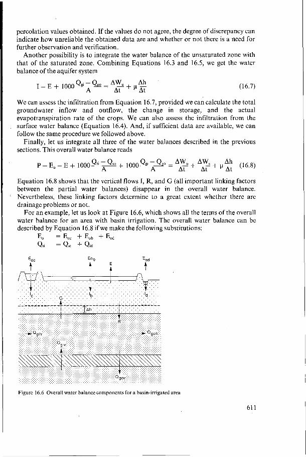
Qsi - Qso + 1000 - -- AwU + S + p- (16.8) P - E, - E + 1000 A

Equation 16.8 shows that the vertical flows I, R, and G (all important linking factors between the partial water balances) disappear in the overall water balance. Nevertheless, these linking factors determine to a great extent whether there are drainage problems or not.

For an example, let us look at Figure 16.6, which shows all the terms of the overall water balance for an area with basin irrigation. The overall water balance can be described by Equation 16.8 if we make the following substitutions:

i

Eo = Eo, + Eo, + Eo, Qsi = Qic + Qid

Eo b A E A

. . . . . . . I . . . . . . . . . . . . . . . . . . . . . . . . . . . . . . . . . . . . . . . . . . . . . . . . . . . . . . . . . . . . . c . . . . . . . . . . . . . . . d . . . . . . . . . . . . . G.'.'.'.'.'.'. . . . . . . . . . . . . . . . . . . . . . . . . . . . . . . . . . . . . . . . . . . . .

Figure 16.6 Overall water balance components for a basin-irrigated area

61 1

When water balances are assessed for a hydrologic year, changes in storage in the various partial water balances can often be ignored or reduced to zero if the partial balances are based on long-term average conditions. In Equations 16.3 to 16.8, the sum of the various inflow components then equals the sum of the various outflow components. Drainage designers use this concept of steady state frequently. Their reasons for doing so are explained in Chapter 17.

16.2.6 Practical Applications

Water balance analyses are particularly useful in land reclamation and drainage projects because they provide insight into: - The sources of local groundwater flow, i.e. the difference between the outflow and

inflow of groundwater in the study area; - The portions of rainfall and irrigation water that infiltrate at the land surface,

evaporate from the surface or from the unsaturated zone, or leave the surface as overland flow;

- The quantity of, and the monthly or annual changes in, groundwater flow; - The quantity of groundwater that must be drained artificially to maintain the

watertable at a suitable depth, i.e. the drainable surplus.

We can ask ourselves if the knowledge we gain by investigating an experimental plot or a tract of several hectares is valid for the rest of the area under study (e.g. a large river basin or a delta plain). The answer is ‘no’ because throughout the river basin there are spatial variations in rainfall, evaporation, land use, soil, and hydrogeological conditions. The best way to obtain the water balance for the greater area is to divide the basin into hydrogeological sub-areas. The division should be based on watertable contour maps of the aquifer system and on well hydrographs. Variations in the spacing of the watertable contours reflect differences in the lithology of the aquifer and thus in the transmissivity. An analysis of the available well hydrographs makes it possible to select those wells whose water level fluctuations are similar. With this information, we can distinguish the hydrogeological sub-areas whose watertables react similarly to the processes of groundwater recharge and discharge. If we assess monthly water balances for these sub-areas, and then add up all the corresponding components of the balances, we obtain the annual water balance for the entire basin. These basin discretizations require sufficient and accurate data on the watertable fluctuations throughout the basin, on the specific yield of the unsaturated zone, on the thickness and hydraulic conductivity of the saturated zone, and on soil water content. They also require a network of stream-gauging stations to supply accurate data on the surface water inflow and outflow of the sub-areas.

A river catchment usually consists of a network of natural drainage channels that eventually join the main river. Each of these channels drains a certain area (sub-catchment). Because, over the catchment, there are variations in rainfall

612

distribution, soil and hydrogeological conditions, and land use and vegetation, the sub-catchments react differently during a hydrologic event (e.g. a rainstorm). Figure 16.7 illustrates the reactions of four minor catchments in a rainstorm. The peak flows show not only a marked difference, but also a time lag.

The river runoff depends not only on the hydrology of the catchment, but also on the distribution and intensity of the rainfall, and on the evapotranspiration and storage capacity of the unsaturated zone. In the humid climates of the western hemisphere, the winter season is characterized by low evapotranspiration and a fairly regularly distributed rainfall, whereas in summer evapotranspiration is high and rainfall is irregular. This means that the relation between rainfall and peak runoff is better in winter than in summer.

When considering the soil water content, we must be aware that different soil types have different water retention curves (Figure 16.8). These curves characterize the ability of the soil to retain water during gravity drainage or drying. We must also be aware of the difference in the relation between capillary flux and soil water content when a soil is absorbing water through infiltration and when it is losing water through drainage. One reason for this difference (hysteresis) is the entrapment of air in the soil during the wetting period, which means that the pores of the soil do not completely fill with water even when the capillary flux is zero.

In most soils, the relation between depth to the watertable and soil water storage is fairly direct, which makes it possible to use these relations to estimate the soil water

rainfall in mm

river runofl i n m m l 3 h

4 5 6 7 December 1965

Figure 16.7 River hydrographs of four minor catchments recorded for the same rainstorm (after Colenbrander 1970)

61 3

height above the watertable in m 3.0

2 0

1 .o

0

. . . . . . . . . . . . . . . . . . . . . . . . . . . . . . . . . . . . . . . . . . . . . . . . . . . . . . . . . . . . . . . . . . . . . . . . . . . . . . . . . . . . . . . 1; i :; I : I ; ; ;:: I ; ;I:. : .: .:. : .:. : .:. : .: .: .: .: .: .: . . . . . . . . . . . . . . . . . . . . . . . . . . . . . . . . . . . . . . . . . . . . . .

. . . . . . . . . . . . . . . . . . . . . . . . . . . . . . . . . . . . . . . . . . . . . . . . . . . . . . . . . . . . . . . . . . . . . . . . . . . . . . . . . . . . . . . . . . . . . . . . . . . . . . . . . . . . . . . . . . . . . . . . . . . . . . . . . . . . . . . . . . . . . . . . .

. . . . . . . . . . . . . . . . . . . . . . . . . . . . . . . . . . . . . . . . . . . . . . . . . . . . . . . . . . . . . . . . . . . . . . . . . . . . . . . . . . . . . . . . . . . . . . . . . . . . -I

volumetric soil moisture content, q

Figure 16.8 Typical equilibrium distribution of water in soils above the watertable A: in homogeneous soils B: in stratified soil

content. We can find the value of the specific yield or drainable pore space of the soil for different depths from the slope of the curves. The specific yield is defined in Chapter 2 as the change in soil water content divided by the change in watertable. The specific yield at equilibrium soil water content varies with the type of soil, ranging commonly from 5 to 15 per cent. The equilibrium soil water content is the water content of the soil at which the suction corresponds with the height above the watertable. We can estimate the change in soil water content from the change in watertable by assuming a constant specific yield (say 10% in sandy soils). In most soils, however, the specific yield is not constant, but variable according to the groundwater depth (Table 16.2).

The specific yield can be derived from soil water characteristics (pF curves), and from the known amount of water released from or added to storage and the corresponding change in watertable. A prerequisite to these calculations is that the soil water content before and after the change in watertable must correspond with the equilibrium soil

Table 16.2 Specific yield of two soil types at different watertable depths

Watertable depth cm

~~

Specified yield %

Marine clay ~

Loamy sand ~~

30 5.4 22.3 50 5.1 19.5 70 4.9 16.8

100 4.3 13.0

614

water content. So it is advisable to measure the soil water content, even when the water deficit of the soil profile and the evapotranspiration are so small as to be negligible. Only then will it approach the equilibrium soil water content.

Direct measurements of soil water content by neutron probing are preferable to calculations from p F curves. The soil water content derived from p F curves is higher than that obtained by neutron probing because pF curves assume that equilibrium soil water conditions prevail (Figure 16.9). The calculations for the shallow soil layers are too high because of the entrapped air in some of the pores. Measurements with a neutron probe automatically account for entrapped air in the soil profile (Chapter 11). For the saturated zone, the discrepancies between measured and calculated soil water contents are much smaller because little or no air is present in soil that is permanently waterlogged.

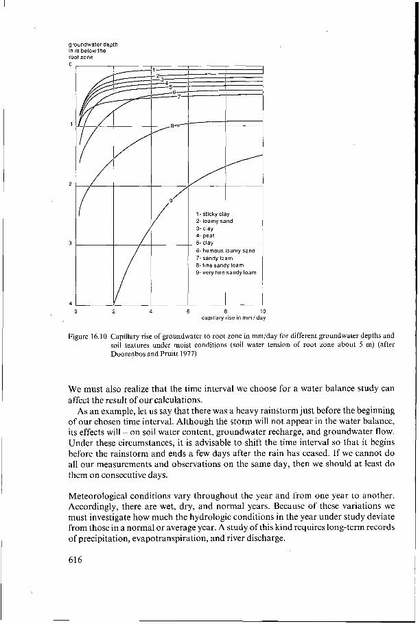
Finally, we must realize that the depth of the watertable plays a crucial role in evaluating the discharge from an area. If the groundwater is deep, say many metres below the ground surface, we only have to consider the groundwater inflow and outflow for a specified area. In areas with shallow watertables, however, say less than 3 m below the ground surface, there is considerable groundwater outflow due to capillary rise, i.e. an upward flux from the watertable, which can bring the groundwater to the land surface, where it is then lost to evaporation (if the soil is barren) or to evapotranspiration (if the soil has a vegetative cover). The loss of groundwater to the rootzone of crops can also be great, especially in the dry season, when the soil water storage is partly depleted. But the size of these losses depends on the soil type (Figure 16.10). Very fine sandy loam, for example, has a very high capacity for capillary rise into the rootzone.

ground water depth in cm

50

350 400 450 500 550 moisture content in mm

Figure 16.9 The relation between groundwater depth and water content of sandy humus podzol soils in the eastern part of The Netherlands. Curve a determined by neutron logging, curve bcalculated from pF-curves (after Colenbrander 1970)

615

groundwater depth in m below the root zone

O 2 4 6 8 10 capillary rise in mmlday

Figure 16.10 Capillary rise of groundwater to root zone in "/day for different groundwater depths and soil textures under moist conditions (soil water tension of root zone about 5 m) (after Doorenbos and Pruitt 1977)

We must also realize that the time interval we choose for a water balance study can affect the result of our calculations.

As an example, let us say that there was a heavy rainstorm just before the beginning of our chosen time interval. Although the storm will not appear in the water balance, its effects will - on soil water content, groundwater recharge, and groundwater flow. Under these circumstances, it is advisable to shift the time interval so that it begins before the rainstorm and ends a few days after the rain has ceased. If we cannot do all our measurements and observations on the same day, then we should at least do them on consecutive days.

Meteorological conditions vary throughout the year and from one year to another. Accordingly, there are wet, dry, and normal years. Because of these variations we must investigate how much the hydrologic conditions in the year under study deviate from those in a normal or average year. A study of this kind requires long-term records of precipitation, evapotranspiration, and river discharge.

616

16.2.7 Equations for Water and Salt Balances

So far, we have considered only the movement of groundwater. We shall now discuss the quality of groundwater, which is determined by the amount and nature of the solutes it contains. The movement and build-up of these solutes (e.g. salt and chemical and organic pollutants) can lead to the salinization and even to the pollution of the groundwater and the soil. These problems can, in turn, effect aquatic ecosystems, crop yields, and ultimately human health. We can establish salt balances by coupling the movement of salts and other solutes to the movement of the groundwater. The equations for these calculations are discussed below.

Groundwater quality is a major factor in drainage studies. Drainage water is sometimes re-used for irrigation and other purposes, either in the project area or in downstream areas. When this water is re-used, it is necessary to estimate for the particular drainage system the quantities of salts and other solutes that are being swept along with the drain effluent. These amounts are usually estimated from salt balances.

The salt balances discussed here focus on salts that are present in both a liquid and a solid state and that, in solution, will move at the same density and at the same velocity as water. The salt balances deal with the major elements in natural waters, namely the cations calcium, magnesium, sodium, and potassium, and the anions bicarbonate, carbonate, sulphate, and chloride. Minor elements like boron, fluoride, and nitrate, and chemicals like pesticides and herbicides are excluded. By and large, it is the major elements that control the chemical character of the water. Their concentrations are expressed in tons/ha.

We can say that the total water balance of an area over a long period of time is in a steady state. The salt balance, however, is not in a steady state. Salt enters the system at the land surface through the inflow of canal water or surface water and through precipitation. It leaves the system through surface drains or field runoff. Salt can also enter the system through groundwater inflow and leave through groundwater outflow. Changes in salt storage are determined by the surface water conditions, by the soil moisture, and by the groundwater regime. Salt ions need different periods of time to travel through the system, depending on the length of the path they take. Salt ions in the groundwater zone follow the same paths as water molecules - along the streamlines towards the drains or pumped wells. These streamlines may reach far below drain depth (Chapter S), mobilizing the salts and other solutes that occur in the deeper parts of the aquifer.

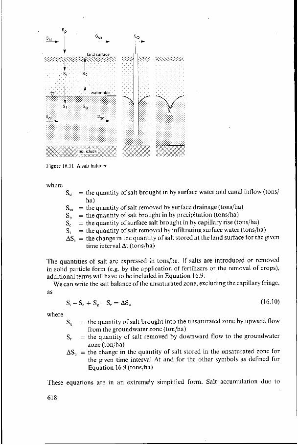
It is possible to derive partial salt balances for the land surface, the unsaturated zone, and the groundwater zone. To do this, let us consider a column of soil. This column extends from the land surface to the impermeable base and is bounded on both sides by imaginary vertical planes. Let us further assume that the hydraulic system of the column is in a steady state, so that the watertable is constant (Figure 16.1 1).

If we also assume that there is no addition or removal of salts by the wind, and that evaporation and crop evapotranspiration occur at the land surface, the balance of soluble salts at the land surface is

S,i - S,, + S, + S, - Si = AS, (1 6.9)

617

SP sso 4 ."-I land surlace

. . . .+,:;,.,. I . . . . . . . . . . . . . . . . . . . . . . . . . . . . . . . . . . . . . . . . . . . . .

. . . S . . . . . s . . . . , . . . C ' . ~ . ' . ' . ' . ' . ' . . . . . . . . . . . . . . . .

Figure 16.1 1 A salt balance

where

I t

S,, = the quantity of salt brought in by surface water and canal inflow (tons/

S,, = the quantity of salt removed by surface drainage (tons/ha) S, = the quantity of salt brought in by precipitation (tons/ha) S, = the quantity of surface salt brought in by capillary rise (tonsiha) Si = the quantity of salt removed by infiltrating surface water (tons/ha) AS, = the change in the quantity of salt stored at the land surface for the given

ha)

time interval At (tons/ha)

The quantities of salt are expressed in tons/ha. If salts are introduced or removed in solid particle form (e.g. by the application of fertilizers or the removal of crops), additional terms will have to be included in Equation 16.9.

We can write the salt balance of the unsaturated zone, excluding the capillary fringe, as

( 1 6.1 O) Si - S, + S, - SI = AS,

where S, = the quantity of salt brought into the unsaturated zone by upward flow

from the groundwater zone (ton/ha) SI = the quantity of salt removed by downward flow to the groundwater

zone (ton/ha) AS, = the change in the quantity of salt stored in the unsaturated zone for

the given time interval At and for the other symbols as defined for Equation 16.9 (tons/ha)

These equations are in an extremely simplified form. Salt accumulation due to

618

evaporation and crop evapotranspiration, for example, is more complicated than the equations would lead us to believe here. It occurs both at the surface and in the rootzone, and itsdistribution decreases with depth. Nevertheless, it is possible to adjust these and other components in the salt balance with a multi-layered soil column (e.g. the four-layered rootzone in Section 15.5.1 of Chapter 15). With these adjustments, the component.S, will not appear in the surface salt balance (Equation 16.9), but in the salt balance of the subsequent soil layers or the compartments in the upper soil profile.

The salt balance of the groundwater zone, including the capillary fringe, is

S, - S, + S,i - S,, - S, = ASg

Sfii = the quantity of salt brought in by the inflow of groundwater (tons/ha) S,, = the quantity of salt removed by the outflow of groundwater (ton/ha) S, = the quantity of salt removed by subsurface drainage flow, either by

tubewells or subsurface drains (tons/ha) ASg = the change in the quantity of salts stored in the groundwater zone for

the given time interval At and for the other symbols as defined for Equation 16.10 (tons/ha)

(16.1 1)

where

If the quality of the groundwater is heterogeneous in a vertical direction, we can divide the saturated zone into horizontal compartments, as we did when making the water balance.

If we integrate the three salt balances, neglecting S, (because the quantity of salt introduced with precipitation is usually small compared with the other components), we obtain the total salt balance

( 1 6.1 2)

In all these balances, the change in salt storage refers to salt in solution and salt solids. The storage of highly soluble salts in the effective zone of full saturation, i.e. in surface waters and in the groundwater zone and the capillary fringe, is often assumed to be constant. Note that these equations omit the precipitation and solution of slightly soluble salts, and that the effect of these processes becomes more pronounced at high salt concentrations (Chapter 15).

Factors that we must consider when investigating the salt build-up in drainage projects include: - The concentration of salt in the groundwater; - The concentration of salt in the soil layers above the watertable; - The depth and spacing of the drains; - The rate and depth of pumping of tubewells.

S,i - S,, + S,i - S,, - S, = AS, + ASu + ASg

The first two factors are fixed by nature or by the past and present land use of the project area. The other factors are engineering variables.

In areas with a thick unconfined aquifer (the impermeable layer is at great depth), it is possible to limit an assessment of the total balance to the upper part of the aquifer,

619