1/36

P �i ?

22333ML232

Sequential Linear Cone Programming

(SLCP)

... and Sensitivity of SDP’s

Chemnitz, Nov. 9, 2004

R.W. Freund, F. Jarre

2/36

P �i ?

22333ML232

Survey

Linear Semidefinite Optimization

• Notation

• Sensitivity Analysis

2/36

P �i ?

22333ML232

Survey

Linear Semidefinite Optimization

• Notation

• Sensitivity Analysis

Recent Results on Nonlinear Semidefinite Optimization

• Application (Positive Real Lemma)

• Generalized Sensitivity Result

• An SLCP Method

3/36

P �i ?

22333ML232

Notation

Sn: The space of symmetric n× n-matrices

X � 0, (X � 0): X ∈ Sn is positive semidefinite (positive definite).

Standard scalar product on the space of n× n-matrices

〈C,X〉 := C •X := trace(CTX) =∑i,j

Ci,jXi,j

inducing the Frobenius norm,

X •X = ‖X‖2F .

4/36

P �i ?

22333ML232

Notation (continued)

For given symmetric matrices A(i) a linear map A from Sn to IRm is given by

A(X) =

A(1) •X

...

A(m) •X

.The adjoint operator A∗ is given by

A∗(y) =m∑i=1

yiA(i).

Linear Semidefinite Program in Standard Form:

minimize C •X where A(X) = b

X � 0

5/36

P �i ?

22333ML232

Duality

If there exists X � 0 with A(X) = b (strict feasibility), then

(P ) inf C •X s.t. A(X) = b, X � 0

(D) = sup bTy s.t. A∗(y) + S = C, S � 0.

If (P ) and (D) have strictly feasible solutions, then the opti-mal solutions X and y, S of both problems exist and satisfy the

equation

XS = 0.

(Converse is true even when Slaters condition is violated.).

6/36

P �i ?

22333ML232

Today, linear SDPs are well analyzed and there exists

Numerically efficient

(and polynomial)

public domain software

for linear semidefinite programs,

e.g. SEDUMI by Jos Sturm (∗1971, †2003).

7/36

P �i ?

22333ML232

Motivation:

Plan to solve a nonlinear SDP by a sequence of (approximating)

linear SDPs.

Need to understand how the optimal solution of the linear SDP

changes when its data is perturbed slightly.

8/36

P �i ?

22333ML232

A sensitivity result for linear SDPs

Uniqueness-assumption:

Data D of a pair (P ) and (D) of primal and dual linear semidefinite programs:

D = [A, b, C] with A : Sn → IRm, b ∈ IRm, C ∈ Sn.

Assume that (P ) and (D) satisfy Slater’s condition, and that X ∈ Sn and

y ∈ IRm, S ∈ Sn are unique and strictly complementary solutions of (P )

and (D), that is,

A(X) = b, X � 0,

A∗(y) + S = C, S � 0,

XS = 0, X + S � 0.

9/36

P �i ?

22333ML232

Theorem (Freund & J. 2003)

If the data of (P ) and (D) is changed by sufficiently small per-

turbations

∆D = [∆A,∆b,∆C],

then the optimal solutions X(D), y(D), S(D) of the semidefinite

programs are differentiable (analytic) functions of the perturbati-

ons, i.e.

X(D + ∆D) = X(D) +DDX[∆D] +O(‖∆D‖2).

10/36

P �i ?

22333ML232

Furthermore, the directional derivatives

X := DDX[∆D], y := DDy[∆D], and S := DDS[∆D],

of the solution X(D), y(D), S(D) satisfy

A(X) = ∆b−∆A(X),

A∗(y) + S = ∆C −∆A∗(y),

XS + XS = 0.

The last line can be equivalently rewritten as

SX + SX + XS + XS = 0.

More general theory in Bonnans and Shapiro (2000).

11/36

P �i ?

22333ML232

Idea of Proof:

1) Slater and continuity:

The perturbed problem must have a solution.

2) Subtract optimality conditions and take limit:

We get precisely the statement of the theorem.

3) It remains to be shown that this system is “nonsingular”.

(It is an overdetermined system just by the number of

equations and unknowns.)

12/36

P �i ?

22333ML232

Idea of Proof: (continued)

By complementarity, XS = 0 = SX, and thus the matrices X � 0 and S � 0

commute. This guarantees that there exists a unitary matrix U and diagonal

matrices

Λ = Diag (λ1, λ2, . . . , λn) � 0 and Σ = Diag (σ1, σ2, . . . , σn) � 0

such that

X = UΛUT and S = UΣUT .

Partition

λ1, λ2, . . . , λk > 0 and σk+1, σk+2, . . . , σn > 0.

Transform so that, without loss of generality, X = Λ, S = Σ and consider the

upper triangular part Πup(∆XΣ + Λ∆S) = 0,

along with A(∆X) = 0 and A∗(∆y) + ∆S = 0.

13/36

P �i ?

22333ML232

Idea of Proof: (continued II)

Using the structure of the equation and uniqueness of the optimal solution

shows that this system has only the zero solution.

14/36

P �i ?

22333ML232

Idea of Proof: (last)

4) Implicit function theorem ... (Done)

Key was to identify a nonsingular part of the overdetermined sy-

stem – that can also be used numerically.

Proof does not use the central path or interior-point techniques.

5) Upper semicontinuity of optimal solutions for more general cone

programs was established by Robinson (1982).

Here we consider special (linear semidefinite) cone programs.

There is a simple example that this theorem does not hold for

strictly complementary solutions of more general cone programs:

15/36

P �i ?

22333ML232

Example

16/36

P �i ?

22333ML232

Maximize x1 subject to these (infinitely many) linear constraints.

Add the redundant constraint x1 ≤ 1. (All other constraints are

‘facet defining’.)

Then the optimal solution is unique, strictly complementary, but

the only active constraint is the redundant constraint x1 ≤ 1.

If the objective gradient (1, 0)T is changed a bit, the optimal so-

lution jumps between the “vertices” close to (1, 0)T . In particular,

it is not differentiable.

From this set form a closed convex cone in IR3 to have a conic

program.

17/36

P �i ?

22333ML232

Corollary

Any step X + tX for t 6= 0 is (typically) infeasible in the sense

that X + tX 6� 0. In some applications the following formula for

the second directional derivative X := 12D

2DX(D)[∆D,∆D] may

be useful:

A(X) = −∆A(X),

A∗(y) + S = −∆A∗(y),

XS + XS = −XS.

This is the same system matrix as for the first derivative with

different right hand side.

18/36

P �i ?

22333ML232

Note:

When X = UΛUT where the diagonal matrix Λ has a leading

nonzero diagonal block Λ1 as in the preceeding proof, then X has

the following structure:

X = U

A B

BT 0

UT ,

and X has the structure

X = U

∗ ∗∗ BTΛ−1

1 B

UT .

Setting ∗ = 0 yields a minimum norm second order correction

towards the positive semidefinite cone maintaining the multiplicity

of the zero eigenvalue (up to third order terms).

19/36

P �i ?

22333ML232

Nonlinear SDP’s

Many important applications:

Truss design with buckling constraints

(Ben Tal, J., Nemirovski, Kocvara, Zowe)

Robust optimization

(Ben Tal and Nemirovski)

Passivity of Pade-approximations in circuit design, positive real

lemma.

(Freund and J.)

Applications in stochastics, ...

Often obtained but sometimes “nearly unsolvable”.

20/36

P �i ?

22333ML232

Circuit design (talk of R.W. Freund)

The physical behavior of a (planned) VLSI design is given by a system of the

form

Ex = Ax+Bu

y = CTx+Du

The system is passive (does not generate energy). Generalized version

of the positive real lemma for descriptor systems (Freund and J. 2003):

Under mild conditions there exists a matrix P such thatPA+ ATP PB − CBTP − CT −D −DT

� 0

and

ETP = P TE � 0.

21/36

P �i ?

22333ML232

In applications, A and E are not known exactly. Instead some Pade-approximation

A, E of A,E is given with an optimal order of approximation. However, the

system with A, E is typically not passive.

To maintain a high order of approximation, a structured low-rank

perturbation A(x), E(x) of A and E is searched for such that

∃ P : Z(x, P ) :=

PA(x) + A(x)TP PB − CBTP − CT −D −DT

� 0

and

E(x)TP = P TE(x) � 0.

This leads to the nonlinear SDP:

minimizex,P

{λmax(Z(x, P )) | subject to E(x)TP = P TE(x) � 0}.

22/36

P �i ?

22333ML232

First Approach:

A Predictor Corrector Barrier Approach

• using ellipsoidal trust regions of variing shape and radii

(considerably more expensive than standard trust region steps)

Make cheaper subproblems once the overall method converges rapidly.

• and adaptive step length control in predictor step (depending

on the difficulty for approximately solving the previous corrector

step).

This framework had worked reliably for any convex problem tried

so far.

Good results for ramdomly generated BMIs (Fukuda and Kojima).

Devastating number of iterations for BMIs from VLSI design.

23/36

P �i ?

22333ML232

Nonlinear semidefinite program:

minimizex∈IRn bTx subject to B(x) � 0,

c(x) ≤ 0,

d(x) = 0.

For this talk: Omit c(x) and d(x).

L(x, Y ) := bTx+ B(x) • Y,g(x, Y ) := ∇xL(x, Y ) = b+∇x (B(x) • Y ) ,

H(x, Y ) := ∇2xL(x, Y ) = ∇2

x (B(x) • Y ) .

24/36

P �i ?

22333ML232

Notation

We assume that the nonlinear function B : IRn → Sm is at least C2-differentiable

and denote by

B(i)(x) :=∂

∂xiB(x) and B(i,j)(x) :=

∂2

∂xi∂xjB(x), i, j = 1, 2, . . . , n,

the first and second partial derivatives of B, respectively. For each x ∈ IRn,

the derivative DxB at x induces a linear function DxB(x) : IRn → Sm, which

is given by

DxB(x)[∆x] :=n∑i=1

(∆x)iB(i)(x) ∈ Sm for all ∆x ∈ IRn.

In particular,

B(x+ ∆x) ≈ B(x) +DxB(x)[∆x], ∆x ∈ IRn,

is the linearization of B at the point x. For any linear function A : IRn → Sm,

we have

DxA(x)[∆x] = A(∆x) for all x, ∆x ∈ IRn.

25/36

P �i ?

22333ML232

Notation (continued)

For any fixed matrix Y ∈ Sm, the map x 7→ B(x)•Y is a scalar-valued function

of x ∈ IRn. Its gradient at x is given by

∇x (B(x) • Y ) = (Dx (B(x) • Y ))T =

B(1)(x) • Y

...

B(n)(x) • Y

∈ IRn

and its Hessian by

∇2x (B(x) • Y ) =

B(1,1)(x) • Y · · · B(1,n)(x) • Y

......

B(n,1)(x) • Y · · · B(n,n)(x) • Y

∈ Sn.In particular, for any linear function A : IRn → Sm, we have

∇x (A(x) • Y ) = A∗(Y ).

26/36

P �i ?

22333ML232

Optimality condition:

B(x) + S= 0,

g(x, Y ) = 0,

Y S= 0,← µI

Y, S� 0.

Linearization of the optimality condition (which is a “nonsingular” condition):

Find S, ∆x and ∆Y such that

B(xk) +DxB(xk)[∆x] + S= 0,

b+Hk∆x+∇x(B(xk) • (Y k + ∆Y )) = 0,

(Y k + ∆Y k)S= 0, bilinear

Y k + ∆Y, S� 0. nonlinear inequalities

27/36

P �i ?

22333ML232

Equivalent quadratic semidefinite program

minimize bT∆x+ 12(∆x)THk∆x

subject to ∆x ∈ IRn : B(xk) +DxB(xk)[∆x] � 0.

If H is positive semidefinite

the quadratic objective function can be rewritten as

• a convex quadratic constraint in plain primal methods,

• a second order constraint (SEDUMI, Jos Sturm).

28/36

P �i ?

22333ML232

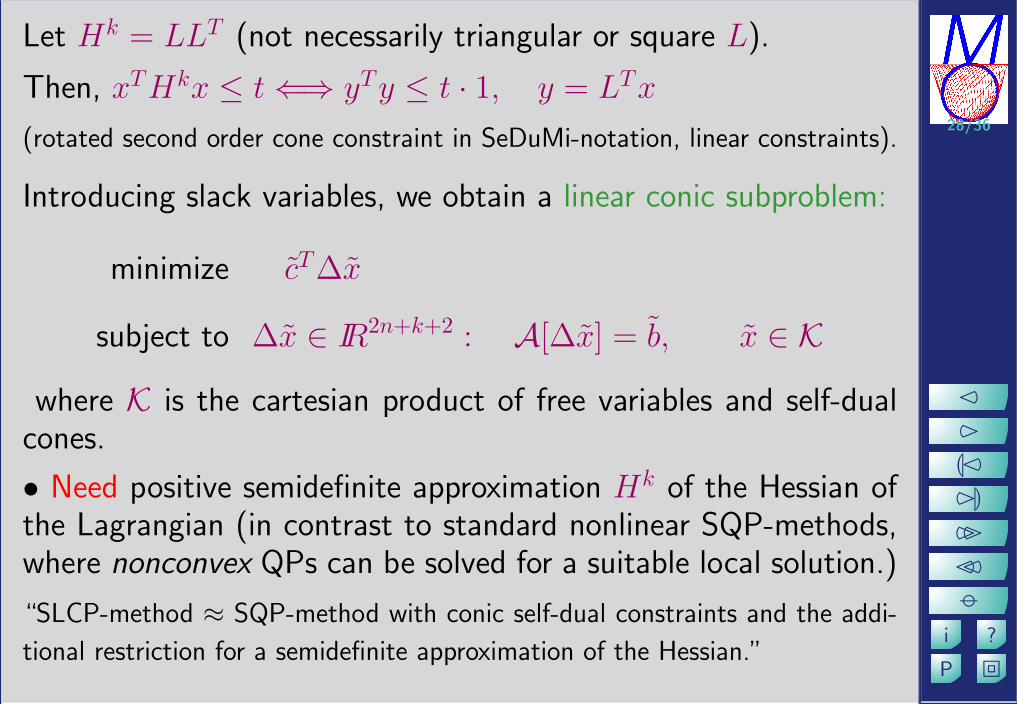
Let Hk = LLT (not necessarily triangular or square L).

Then, xTHkx ≤ t⇐⇒ yTy ≤ t · 1, y = LTx

(rotated second order cone constraint in SeDuMi-notation, linear constraints).

Introducing slack variables, we obtain a linear conic subproblem:

minimize cT∆x

subject to ∆x ∈ IR2n+k+2 : A[∆x] = b, x ∈ K

where K is the cartesian product of free variables and self-dualcones.

• Need positive semidefinite approximation Hk of the Hessian ofthe Lagrangian (in contrast to standard nonlinear SQP-methods,where nonconvex QPs can be solved for a suitable local solution.)

“SLCP-method ≈ SQP-method with conic self-dual constraints and the addi-

tional restriction for a semidefinite approximation of the Hessian.”

29/36

P �i ?

22333ML232

Local quadratic convergence

for unique, strictly complementary local solutions that satisfy a

second order growth condition using exact Hessians.

Outline of Proof:

1) Straightforward (but tedious) generalization of sensitivity ana-

lysis for linear SDP to nonconvex quadratic SDP and to general

nonlinear SDP.

2) Implicit function theorem. #

Sensitivity analysis also in Bonnans and Shapiro, 2000, with more general con-

cept, transversality condition, inf sup compactness condition.

Local analysis and comparison with Augmented Lagrangian:

Fares, Noll, Apkarian (2000)

30/36

P �i ?

22333ML232

In Step 1): Nonconvex quadratic SDP

minimize

{bTx+

1

2xTHx | A(x) + C � 0

}.

Here, A : IRn → Sm is a linear operator;

and the data is D := [A, b, C,H].

31/36

P �i ?

22333ML232

Assumptions:

There exists x with A(x) + C ≺ 0.

There exists a locally unique strictly complementary solution x(D), Y (D)S(D),

A(x) + C + S = 0, S � 0,

b+Hx+A∗(Y ) = 0, Y � 0,

Y S = 0, X + S � 0.

x(D), Y (D)S(D) satisfies a second order growth condition: There exists some

µ > 0 such that for any feasible direction h with hT (b+Hx) = 0 (i.e. where the

objective function is approximately constant) the inequality

hTHh ≥ µ‖h‖2

is true. (Note that the Hessian of the Lagrangian Lq(x, Y ) := bTx+ 12xTHx+

(A(x) + C) • Y coincides with the Hessian H of the objective function since

the constraints are linear.)

32/36

P �i ?

22333ML232

Theorem

If the data D is changed by sufficiently small perturbations

∆D = [∆A,∆b,∆C,∆H],

then the optimal solutions of the perturbed semidefinite programs are diffe-

rentiable functions of the perturbations. Furthermore, the derivatives

x := DDx[∆D], Y := DDY [∆D], and S := DDS[∆D],

of the solution x, Y , S at x, Y , S satisfy

A(x) + S = −∆C −∆A(x),

Hx+A∗(Y ) = −∆b−∆Hx−∆A∗(Y ),

Y S + Y S = 0.

33/36

P �i ?

22333ML232

Consequence

Since the necessary and sufficient optimality conditions of a general nonlinear

SDP, are precisely the same as those for the associated quadratic SDP, (with

H given by the Hessian of the Lagrangian) this sensitivity result generalizes.

Under uniqueness, strict complementarity, and second order growth condition

it can be used to show

• that the size of the “residual” in the SSP sub-problem is of the same order

as the distance to optimality,

• that the SSP step is also of this size,

• and – as the residual after the SSP step is just the linearization error – that

the residual after the SSP step therefore must be “squared”.

34/36

P �i ?

22333ML232

Practical refinements (C. Vogelbusch, in progress)

• BFGS updates for Hk based on augmented Lagrangian

Λ(x, Y ; r) = bTx+r

2

(B(x) +Y

r

)+2

• I − Y • Y2r

.

(When M := B(x) + Yr is invertible, the first derivative of

((M+)2) is given by (LM+)2L−1

|M | where LM(H) = MH +HM is

the Lyapunov operator.)

• Second order correction (to avoid Maratos effect).

• Filter approach.

35/36

P �i ?

22333ML232

Open Questions

• Theoretical rate of convergence when using the exact (or an

approximate) Hessian of the augmented Lagrangian.

• Choice of the penalty parameter.

• Sparsity (so far dense Hessian) — may need to include limited

memory BFGS for Hessian of Lagrangian and different SDP-solver.

(This is completely open, so far work with 40 × 40 systems is

possible, but still in debugging stage.)

• Reformulation of nonlinear SDP to less ill-conditioned form?

36/36

P �i ?

22333ML232

Concluding Remark

• Sensitivity result for nonlinear semidefinite programs.

• This result can be used to derive an elementary and self-contained proof of

local quadratic convergence of the sequential linear conic programming (SLCP)

method (a generalization of the well-known SQP method).

• For interior methods that are applied directly to nonlinear semidefinite pro-

grams, the choice of the symmetrization procedure is considerably more com-

plicated than in the linear case since the system matrix is no longer positive

semidefinite.

• In the SLCP method, the choice of the symmetrization scheme is shifted to

the subproblems and is thus separated from the linearization.