1.3 vector fields and flows. - cds.caltech.edu

1.3 Vector Fields and Flows. 21

1.3 Vector Fields and Flows.

This section introduces vector fields on Euclidean space and the flows theydetermine. This topic puts together and globalizes two basic ideas learnedin undergraduate mathematics: the study of vector fields on the one handand differential equations on the other.

Definition 1.3.1. Let r ≥ 0 be an integer. A Cr vector field on Rn is amapping X : U → Rn of class Cr from an open set U ⊂ Rn to Rn. The setof all Cr vector fields on U is denoted by Xr(U) and the C∞ vector fieldsby X∞(U) or X(U).

We think of a vector field as assignning to each point x ∈ U a vectorX(x) based (i.e., bound) at that same point.

Example. Consider the force field determined by Newton’s law of gravi-tation. Here the set U is R3 minus the origin and the vector field is definedby

F(x, y, x) = −mMG

r3r,

where m is the mass of a test body, M is the mass of the central body, Gis the constant of gravitation, r is the vector from the origin to (x, y, z),and r = (x2 + y2 + z2)1/2; see Figure 1.3.1.

Figure 1.3.1. The gravitational force field.

!

22 1. Basic Theory of Dynamical Systems

Consider a general physical system that is capable of assuming various“states” described by points in a set Z. For example, Z might be R3 ×R3

and a state might be the position and momentum (q,p) of a particle. Astime passes, the state evolves. If the state is z0 ∈ Z at time t0 and thischanges to z at a later time t, we set

Ft,t0(z0) = z

and call Ft,t0 the evolution operator ; it maps a state at time t0 to whatthe state would be at time t; i.e., after time t− t0 has elapsed. “Determin-ism” is expressed by the law

Ft2,t1 ◦ Ft1,t0 = Ft2,t0 Ft,t = identity,

sometimes called the Chapman-Kolmogorov law .The evolution laws are called time independent when Ft,t0 depends

only on t− t0; i.e.,

Ft,t0 = Fs,s0 if t− t0 = s− s0.

Setting Ft = Ft,0, the preceding law becomes the group property :

Fτ ◦ Ft = Fτ+t, F0 = identity.

We call such an Ft a flow and Ft,t0 a time-dependent flow , or an evo-lution operator. If the system is defined only for t ≥ 0, we speak of asemi-flow .

It is usually not Ft,t0 that is given, but rather the laws of motion . Inother words, differential equations are given that we must solve to find theflow. In general, Z is a manifold (a generalization of a smooth surface), butwe confine ourselves here to the case that Z = U is an open set in someEuclidean space Rn. These equations of motion have the form

dx

dt= X(x), x(0) = x0

where X is a (possibly time-dependent) vector field on U .

Example. The motion of a particle of mass m under the influence of thegravitational force field is determined by Newton’s second law:

md2rdt2

= F;

i.e., by the ordinary differentatial equations

md2x

dt2= −mMGx

r3;

md2y

dt2= −mMGy

r3;

md2z

dt2= −mMGz

r3;


Letting q = (x, y, z) denote the position and p = m(dr/dt) the momentum,these equations become

dqdt

=pm

;dpdt

= F(q)

The phase space here is the open set U = (R3\{0})× R3. The right-handside of the preceding equations define a vector field by

X(q,p) = ((q,p), (p/m,F(q))).

In courses on mechanics or differential equations, it is shown how to in-tegrate these equations explicitly, producing trajectories, which are planarconic sections. These trajectories comprise the flow of the vector field. !

Relative to a chosen set of Euclidean coordinates, we can identify a vec-tor field X with an n-component vector function (X1(x), . . . , Xn(x)), thecomponents of X.

Definition 1.3.2. Let U ⊂ Rn be an open set and X ∈ Xr(U) a vectorfield on U . An integral curve of X with initial condition x0 is a differen-tiable curve c defined on some open interval I ⊂ R containing 0 such thatc(0) = x0 and c′(t) = X(c(t)) for each t ∈ I.

Clearly c is an integral curve of X when the following system of ordinarydifferential equations is satisfied:

dc1

dt(t) = X1(c1(t), . . . , cn(t))

......

dcn

dt(t) = Xn(c1(t), . . . , cn(t))

We shall often write x(t) = c(t), an admitted abuse of notation. Thepreceding system of equations are called autonomous, when X is timeindependent. If X were time dependent, time t would appear explicitlyon the right-hand side. As we have already seen, the preceding systemof equations includes equations of higher order by the usual reduction tofirst-order systems.

Theorem 1.3.3 (Local Existence, Uniqueness, and Smoothness).Suppose that U ⊂ Rn is open and that X is a Cr vector field on U for somer ≥ 1. For each x0 ∈ U , there is a curve c : I → U with c(0) = x0 suchthat c′(t) = X(c(t)) for all t ∈ I. Any two such curves are equal on theintersection of their domains. Furthermore, there is a neighborhood U0 ofthe point x0 ∈ U , a real number a > 0, and a Cr mapping F : U0× I → U ,where I is the open interval ] − a, a [, such that the curve cu : I → U ,defined by cu(t) = F (u, t) is a curve satisfying cu(0) = u and the differentialequations c′u(t) = X(cu(t)) for all t ∈ I.


This theorem has many variants. We refer to Coddington and Levinson[1955] and Hartman [2002] for a thorough discussion of most of them. Forexample, with just continuity of X one can get existence (the Peano exis-tence theorem) without uniqueness. The equation in one dimension givenby x =

√x, x(0) = 0 has the two C1 solutions x1(t) = 0 and x2(t) which is

defined to be 0 for t ≤ 0 and x2(t) = t2/4 for t > 0. This shows that onecan indeed have existence without uniqueness for continuous vector fields.

The proof of the preceding theorem is based on the following.

Theorem 1.3.4 (Local Existence and Uniqueness). Let U ⊂ Rn bean open set, and X : U → Rn be a Lipschitz map; i.e., there is a constantK > 0 such that

‖X(x)−X(y)‖ ≤ K‖x− y‖

for all x, y ∈ U . Let x0 ∈ U and suppose the closed ball of radius b, Bb(x0) ={x ∈ Rn| ‖x− x0‖ ≤ b} lies in U , and that ‖X(x)‖ ≤ M for a constant Mand all x ∈ Bb(x0). Let t0 ∈ R and let α = b/M . Then there is a uniqueC1 curve x(t), t ∈ [t0 − α, t0 + α] such that

x(t) ∈ Bb(x0) and

{x′(t) = X(x(t))x(t0) = x0.

Proof. The conditions x′(t) = X(x(t)), x(t0) = x0 are equivalent to theintegral equation

x(t) = x0 +∫ t

0X(x(s)) ds (1.3.1)

Put x0(t) = x0 and define inductively

xn+1(t) = x0 +∫ t

t0

X(xn(s)) ds.

This process is called Picard iteration. Clearly xn(t) ∈ Bb(x0) for all nand t ∈ [t0 − α, t0 + α] by definition of α. We claim that

‖xn+1(t)− xn(t)‖ ≤ MKn|t− t0|n+1

(n + 1)!. (1.3.2)

To see this, we proceed by induction. For n = 0 this reads

‖x1(t)− x0‖ ≤ M |t− t0|

However, this follows since by definition of x1(t):

x1(t)− x0 =∫ t

t0

X(x0) ds


and since ‖X(x0)‖ ≤ M . Now assume that equation (1.3.2) holds for n. Toprove it for n + 1, we estimate as follows:

‖xn+2(t)− xn+1(t)‖ =∥∥∥∥∫ t

t0

(X(xn+1(s))−X(xn(s))) ds

∥∥∥∥

≤∫ t

t0

(K‖xn+1(s)− xn(s)‖) ds

≤∫ t

t0

(K

MKn|t− t0|n+1

(n + 1)!

)ds

≤ MKn+1|t− t0|n+2

(n + 2)!

and so we have proved equation (1.3.2) for n + 1 as required. Since

MKn

(n + 1)!(t− t0)n+1 ≤ MKn

(n + 1)!αn+1

and the series with these quantities as terms is convergent, we see, writ-ing ‖xn+p − xn‖ as a telescoping sum, that the functions xn(t) form auniformly Cauchy sequence and hence converge uniformly to a continuousfunction x(t). This curve x(t) satisfies the integral equation (1.3.1). Sincex(t) is continuous, the integral equation in fact shows that it is C1 fromthe fundamental theorem of Calculus. This proves existence.

For uniqueness, let y(t) be another solution. By induction we find that‖xn(t) − y(t)‖ ≤ MKn|t − t0|n+1/(n + 1)!; thus, letting n → ∞ givesx(t) = y(t). "

A local existence result may alternatively be proven by making use of thecontraction mapping principle, at least if we “give a little” and assume thatα also satisfies α < 1/K. The idea is to consider the space C of continuouscurves c(t) defined on the closed interval [t0−α, t0+α]. These curves shouldsatisfy c(t0) = x0 and lie in a closed ball of radius b. We consider C as acomplete metric space with the distance function given by the supremumof the distance between two curves. Now we set up a mapping

F : C → C

defined by

F(c(·))(t) = x0 +∫ t

t0

X(c(s)) ds

Then one checks, using the fact that α is less than or equal to b/M that Fmaps C to itself, and the Lipschitz condition on X provides an estimate onF(c1(·))−F(c2(·)) in the sup norm. The condition that α is less than 1/Kshows that F is a contraction. The unique fixed point is the desired integralcurve. Notice, however, that the time of existence given by this technique isnot as good as what was given in the local existence result, Theorem 1.3.4.


Dependence on Parameters and Time. The same argument holds ifX depends explicitly on t and/or on a parameter ρ, is jointly continuous in(t, ρ, x), and is Lipschitz in x uniformly in t and ρ. Since xn(t) is continuousin (x0, t0, ρ) so is x(t), being a uniform limit of continuous functions; thusthe integral curve is jointly continuous in (x0, t0, ρ). 3

The following inequality is of basic importance in not only existence anduniqueness theorems, but also in making estimates on solutions.

Theorem 1.3.5 (Gronwall’s Inequality). Let f, g : [a, b[→ R be con-tinuous and nonnegative. Suppose there is a constant A ≥ 0 such that forall t satisfying a ≤ t ≤ b,

f(t) ≤ A +∫ t

af(s) g(s) ds.

Then

f(t) ≤ A exp(∫ t

ag(s) ds

)for all t ∈ [a, b[.

Proof. First suppose A > 0. Let

h(t) = A +∫ t

af(s) g(s) ds;

thus h(t) > 0. Then h′(t) = f(t)g(t) ≤ h(t)g(t). Thus h′(t)/h(t) ≤ g(t).Integration gives

h(t) ≤ A exp(∫ t

ag(s) ds

).

This gives the result for A > 0. If A = 0, then we get the result by replacingA by ε > 0 for every ε > 0; thus h and hence f is zero. "

Lemma 1.3.6. Let X be as in Theorem 1.3.4. Let Ft(x0) denote thesolution (= integral curve) of x′(t) = X(x(t)), x(0) = x0. Then there is aneighborhood V of x0 and a number ε > 0 such that for every y ∈ V thereis a unique integral curve x(t) = Ft(y) satisfying x′(t) = X(x(t)) for allt ∈ [−ε, ε], and x(0) = y. Moreover,

‖Ft(x)− Ft(y)‖ ≤ eK|t|‖x− y‖.

Proof. Choose V = Bb/2(x0) and ε = b/2M . Fix an arbitrary y ∈ V .Then Bb/2(y) ⊂ Bb(x0) and hence ‖X(z)‖ ≤ M for all z ∈ Bb/2(y). By

3The reader who is familiar with Banach spaces will notice that this proof worksessentially unchanged in that context with Rn replaced by a Banach space. However,one has to be cautious not to think that this will always enable one to deal with partialdifferential equations (such as dealing with equations like the heat equation (∂u/∂t =∇2u) by just choosing the Banach space to be a space of functions.


Theorem 1.3.4 with x0 replaced by y, b by b/2, and t0 by 0, there exists anintegral curve x(t) of x′(t) = X(x(t)) for t ∈ [−ε, ε] and satisfying x(0) = y.This proves the first part. For the second, let f(t) = ‖Ft(x) − Ft(y)‖.Clearly,

f(t) =∥∥∥∥∫ t

0[X(Fs(x))−X(Fs(y))] ds + x− y

∥∥∥∥

≤ ‖x− y‖+ K

∫ t

0f(s) ds,

so the result follows from Gronwall’s inequality. "

This result shows that Ft(x) depends in a continuous, indeed Lipschitz,manner on the initial condition x and is jointly continuous in (t, x). Again,the same result holds if X depends explicitly on t and on a parameter ρ isjointly continuous in (t, ρ, x), and is Lipschitz in x uniformly in t and ρ. Welet F ρ

t,λ(x) be the unique integral curve x(t) satisfying x′(t) = X(x(t), t, ρ)and x(λ) = x. By the remarks following Theorem 1.3.4, F ρ

t,t0(x) is jointlycontinuous in the variables (t0, t, ρ, x), and is Lipschitz in x, uniformly in(t0, t, ρ).

We now want to work towards showing that Ft is Cr if X is. We will dothis first locally and later will also show this for all t for which the flow isdefined.

For the next lemma, recall that by the mean value theorem, a C1-functionis locally Lipschitz.

Lemma 1.3.7. Let X in Theorem 1.3.4 be of class Ck, where 1 ≤ k ≤ ∞,and let Ft(x) be defined as before. Then locally in (t, x), Ft(x) is of classCk in x and is Ck+1 in the t-variable.

Proof. We define ψ(t, x) taking values in the vector space L(Rn, Rn)consisting of the set of linear maps of Rn to Rn (this space is isomorphic toRn2

), to be the solution of the “linearized” or “first variation” equations:

d

dtψ(t, x) = DX(Ft(x)) ◦ ψ(t, x),

with ψ(0, x) = identity, where DX(y) : Rn → Rn is the derivative of Xtaken at the point y. Using the standard Euclidean coordinates, DX is thematrix with entries ∂Xi/∂xj .

Since the vector field ψ ,→ DX(Ft(x)) ◦ ψ on L(Rn, Rn) (dependingexplicitly on t and on the parameter x) is Lipschitz in ψ, uniformly in (t, x)in a neighborhood of every (t0, x0), by the remark following 1.3.6 it followsthat ψ(t, x) is continuous in (t, x).


We claim that DFt(x) = ψ(t, x). To show this, fix t and x, set θ(s, h) =Fs(x + h)− Fs(x), and write

θ(t, h)− ψ(t, x) · h =∫ t

0{X(Fs(x + h))−X(Fs(x))} ds

−∫ t

0[DX(Fs(x)) ◦ ψ(s, x)] · h ds

=∫ t

0DX(Fs(x)) · [θ(s, h)− ψ(s, x) · h] ds

+∫ t

0{X(Fs(x + h))−X(Fs(x))

−DX(Fs(x)) · [Fs(x + h)− Fs(x)]} ds.

Since X is of class C1, given ε > 0, there is a δ > 0 such that ‖h‖ < δimplies the second term is dominated in norm by

∫ t

0ε‖Fs(x + h)− Fs(x)‖ ds,

which is, in turn, smaller than Aε‖h‖ for a positive constant A by lemma1.3.6. By Gronwall’s inequality we obtain

‖θ(t, h)− ψ(t, x) · h‖ ≤ Cε‖h‖,

for a constant C. It follows that DFt(x) · h = ψ(t, x) · h. Thus both partialderivatives of Ft(x) exist and are continuous; therefore Ft(x) is of class C1.

We prove Ft(x) is Cr by induction on r. Begin with the equation definingFt :

d

dtFt(x) = X(Ft(x))

sod

dt

d

dtFt(x) = DX(Ft(x)) · X(Ft(x))

andd

dtDFt(x) = DX(Ft(x)) ·DFt(x)).

Since the right-hand sides are Cr−1, so are the solutions by induction.Thus F itself is Cr. "

Again there is an analogous result for the evolution operator F ρt,t0(x) for a

time-dependent vector field X(x, t, ρ), which depends on extra parametersρ in some other Euclidean space, say Rm . If X is Cr, then F ρ

t,t0(x) is Cr

in all variables and is Cr+1 in t and t0.


Suspenstion Trick. The variable ρ can be easily dealt with by suspend-ing X to a new vector field obtained by appending the trivial differentialequation ρ′ = 0; this defines a vector field on Rn × Rm and the basic exis-tence and uniqueness theorem may be applied to it. The flow on Rn ×Rm

is just Ft(x, ρ) = (F ρt (x), ρ).

Other Approaches and Results. For another more “modern” proofof the basic existence and uniquenss theorem based directly on the implicitfunction theorem applied in function spaces, see Abraham, Marsden, andRatiu [1988]. That alternative proof has a technical advantage: it workseasily for other types of differentiability assumptions on X or on Ft, suchas Holder or Sobolev differentiability; this result is due to Ebin and Marsden[1970].

An interesting result called the rectification theorem, whose proof can befound in Arnold [1983] and Abraham, Marsden, and Ratiu [1988], showsthat near a point x0 satisfying X(x0) -= 0, the flow can be transformedby a change of variables so that the integral curves become straight linesmoving with unit speed. This shows that, in effect, nothing interestinghappens with flows away from equilibrium points as long as one looks atthe flow only locally and for short time.

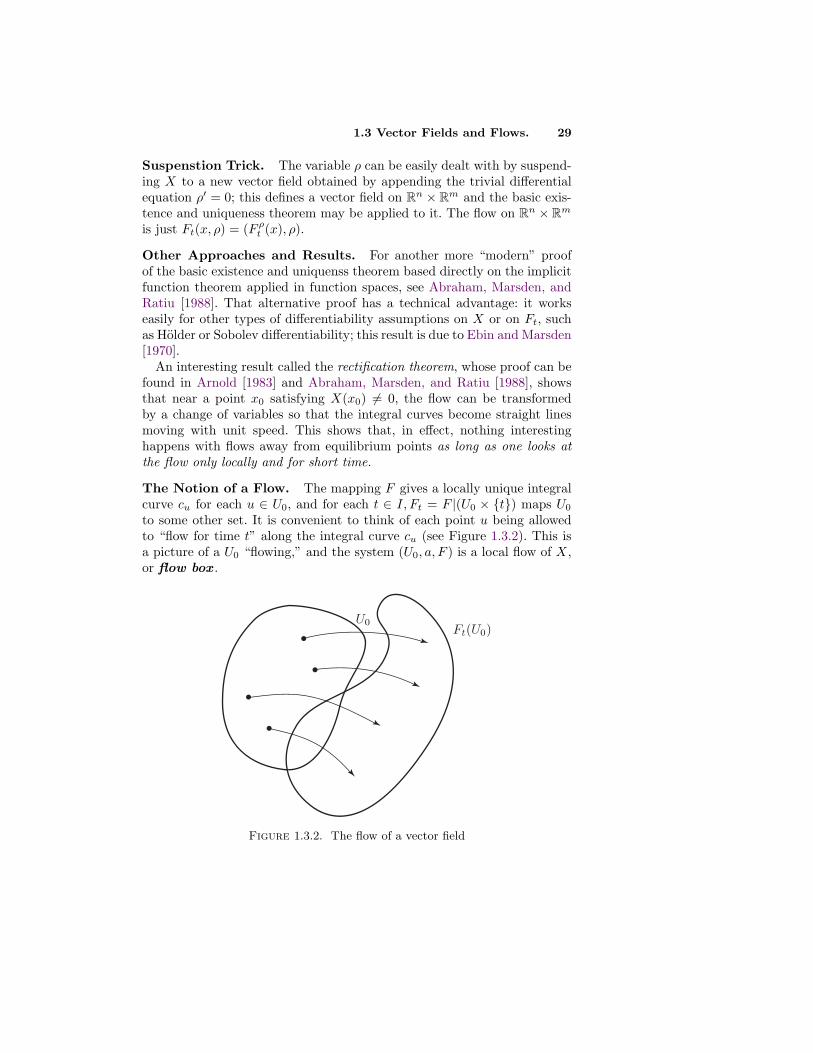
The Notion of a Flow. The mapping F gives a locally unique integralcurve cu for each u ∈ U0, and for each t ∈ I, Ft = F |(U0 × {t}) maps U0

to some other set. It is convenient to think of each point u being allowedto “flow for time t” along the integral curve cu (see Figure 1.3.2). This isa picture of a U0 “flowing,” and the system (U0, a, F ) is a local flow of X,or flow box .

Figure 1.3.2. The flow of a vector field


Global Uniqueness of Integral Curves. While integral curves neednot always exist globally, if they do, they are always unique.

Proposition 1.3.8 (Global Uniqueness). Suppose c1 and c2 are twointegral curves of X in U and that for some time t0, c1(t0) = c2(t0). Thenc1 = c2 on the intersection of their domains.

Proof. Suppose c1 : I1 → U and c2 : I2 → U . Let I = I1 ∩ I2, and letK = {t ∈ I | c1(t) = c2(t)};K is closed since c1 and c2 are continuous. Wewill now show that K is open. From the basic existence and uniquenessresult in Theorem 1.3.3, K contains some neighborhood of t0. For t ∈ Kconsider ct

1 and ct2, where ct(s) = c(t + s). Then ct

1 and ct2 are integral

curves satisfying c1(t) = c2(t). By local uniqueness, they agree on someneighborhood of 0. Thus some neigborhood of t lies in K, and so K isopen. Since I is connnected, K = I. "

Completeness and the Lifetime of a Trajectory. Other global issuescenter on considering the flow of a vector field as a whole, extended as faras possible in the t-variable. In fact, by uniqueness, it makes sense to lookat the largest interval in the positive and negative t-directions on whichone has a solution. We make this formal as follows.

Definition 1.3.9. Given an open set U and a vector field X on U , letDX ⊂ U ×R be the set of (x, t) ∈ U ×R such that there is an integral curvec : I → U of X with c(0) = x with t ∈ I. The vector field X is complete ifDX = U ×R. A point x ∈ U is called σ-complete, where σ = +,−, or ±,if DX ∩ ({x} × R) contains all (x, t) for t > 0, < 0, or t ∈ R, respectively.Let T+(x) (resp. T−(x)) denote the sup (resp. inf) of the times of existenceof the integral curves through x; T+(x) resp. T−(x) is called the positive(negative) lifetime of x.

Thus, X is complete iff each integral curve can be extended so that itsdomain becomes ] − ∞,∞ [; i.e., T+(x) = ∞ and T−(x) = −∞ for allx ∈ U .

Examples

A. Any linear vector field A on Rn is complete. Indeed, the integral curvethrough an initial condition x0 ∈ Rn, namely etAx0 is defined for allt.

B. For U = R2, let X be the constant vector field X(x, y) = (0, 1).Then X is complete since the integral curve of X through (x, y) ist ,→ (x, y + t).

C. On U = R2\{0}, the same vector field is not complete since theintegral curve of X through (0,−1) cannot be extended beyond t = 1;


in fact as t → 1 this integral curve tends to the point (0, 0). ThusT+(0,−1) = 1, while T−(0,−1) = −∞.

D. On R consider the vector field X(x) = 1 + x2. This is not completesince the integral curve c with c(0) = 0 is c(θ) = tan θ and thus itcannot be continuously extended beyond −π/2 and π/2; i.e., T±(0) =±π/2. !

Here are some general properties of flow domains.

Proposition 1.3.10. Let U ⊂ Rn be open and X ∈ Xr(M), r ≥ 1. Then

i DX ⊃ U × {0};

ii DX is open in U × R;

iii there is a unique Cr mapping FX : DX → U such that the mappingt ,→ FX(x, t) is an integral curve at x for all x ∈ U ;

iv for (x, t) ∈ DX , (FX(x, t), s) ∈ DX iff (m, t + s) ∈ DX ; in this case

FX(x, t + s) = FX(FX(x, t), s).

The idea of the proof is as follows. Parts i and ii follow from the localexistence theory. In iii, we get a unique map FX : DX → U by the globaluniqueness and local existence of integral curves: (x, t) ∈ DX when theintegral curve x(s) through x exists for s ∈ [0, t]. We set FX(x, t) = x(t).To show FX is Cr, note that in a neighborhood of a fixed x0 and for smallt, it is Cr by local smoothness. To show FX is globally Cr, first note thativ holds by global uniqueness. Then in a neighborhood of the compact set{x(s)|s ∈ [0, t]} we can write FX as a composition of finitely many Cr mapsby taking short enough time steps so the local flows are smooth. "Definition 1.3.11. Let U ⊂ Rn be open and X ∈ Xr(U), r ≥ 1. Thenthe mapping FX is called the integral of X, and the curve t ,→ FX(x, t)is called the maximal integral curve of X at x. In case X is complete,FX is called the flow of X.

Thus, if X is complete with flow F , then the set {Ft | t ∈ R} is a groupof diffeomorphisms on U , sometimes called a one-parameter group ofdiffeomorphisms. Since Fn = (F1)n (the n-th power), the notation F t issometimes convenient and is used where we use Ft. For incomplete flows, ivsays that Ft ◦ Fs = Ft+s wherever it is defined. Note that Ft(x) is definedfor t ∈ ]T−(x), T+(x)[. The reader should write out similar definitions forthe time-dependent case and note that the lifetimes depend on the startingtime t0.


Criteria for Completeness. There are a number of conditions that areconvenient for checking completeness. We begin with one of the most basicones.

Proposition 1.3.12. Let X be a Cr vector field on an open subset Uof Rn, where r ≥ 1. Let c(t) be a maximal integral curve of X such thatfor every finite open interval ]a, b[ in the domain ]T−(c(0)), T+(c(0))[ ofc, c(]a, b[) lies in a compact subset of U . Then c is defined for all t ∈ R. IfU = Rn, this holds provided c(t) lies in a bounded set.

Proof. It suffices to show that a ∈ I, b ∈ I, where I is the inteval ofdefinition of c. Let Tn ∈ ]a, b[, tn → b. By compactness we can assume somesubsequence c(tn(k)) converges, say, to a point x in U . Since the domain ofthe flow is open, it contains a neighborhood of (x, 0). Thus, there are ε > 0and τ > 0 such that integral curves starting at points (such as c(tn(k))) forlarge k) closer than ε to x persist for a time longer than τ . This serves toextend c to a time greater than b, so b ∈ I since c is maximal. Similarly,a ∈ I. "

A direct corollary of this result relies on the notion of the support ofa vector field. The support of a vector field X defined on an open setU ⊂ Rn is defined to be the closure of the set {x ∈ U |X(x) -= 0} regardedas a subset of Rn.

Corollary 1.3.13. A Cr vector field on an open set U with compactsupport contained in U is complete.

Completeness corresponds to well-defined dynamics persisting eternally.In some circumstances (shock waves in fluids and solids, singularities ingeneral relativity, etc.) one has to live with incompleteness or overcome itin some other way. Because of its importance we give two additional criteria.In the first result we use the notation X[f ] = df ·X for the derivative of fin the direction X. Here f : U → R and df stands for the derivative map.In standard coordinates on Rn,

df(x) =(

∂f

∂x1, . . . ,

∂f

∂xn

)and X[f ] =

n∑

i=1

Xi ∂f

∂xi.

Proposition 1.3.14. Suppose X is a Cr vector field on Rn, and f :Rn → R is a C1 proper map; that is, if {xn} is any sequence in Rn suchthat f(xn) → a, then there is a convergent subseqence {xn(i)}. Supposethere are constants K, L ≥ 0 such that

|X[f ](m)| ≤ K|f(m)| + L for all m ∈ E.

Then the flow of X is complete.


Proof. From the chain rule we have (∂/∂t)f(Ft(m)) = X[f ](Ft(m)), sothat

f(Ft(m))− f(m) =∫ t

0X[f ](Fτ (m)) dτ

Applying the hypothesis and Gronwall’s inequality we see that |f(Ft(x))|is bounded and hence relatively compact on any finite t-interval, so as f isproper, a repetition of the argument in the proof of 1.3.12 applies. "

Proposition 1.3.15. Let X be a Cr vector field on Rn. Let σ be anintegral curve of X. Assume ‖X(σ(t))‖ is bounded on finite t-intervals.Then σ(t) exists for all t ∈ R.

Proof. Suppose ‖X(σ(t))‖ ≤ A for t ∈ ]a, b[ and let tn → b. For tn < tmwe have

‖σ(tn)− σ(tm)‖ ≤∫ tm

tn

‖σ′(t)‖ dt =∫ tm

tn

‖X(σ(t))‖ dt ≤ A|tm − tn|.

Hence σ(tn) is a Cauchy sequence and therefore, converges. Now argue asin 1.3.12. "

Examples

A. Let X be a Cr vector field, r ≥ 1, on the manifold U admitting a firstintegral , i.e., a function f : U → R such that X[f ] = 0. If all levelsets f−1(r), r ∈ R are compact, X is complete. Indeed, each integralcurve lies on a level set of f so that the result follows by Proposition1.3.14.

B. SupposeX(x) = A · x + B(x),

where A is a linear operator of Rn to itself and B is sublinear ; i.e.,B : Rn → Rn is Cr with r ≥ 1 and satisfies ‖B(x)‖ ≤ K‖x‖+ L forconstants K and L. We shall show that X is complete. Let x(t) bean integral curve of X on the bounded interval [0, T ]. Then

x(t) = x(0) +∫ t

0(A · x(s) + B(x(s))) ds

Hence

‖x(t)‖ ≤ ‖x(0)‖∫ t

0(‖A‖+ K)‖x(s)‖ ds + Lt.

By Gronwall’s inequality,

‖x(t)‖ ≤ (LT + ‖x(0)‖)e(‖A‖+K)t.


Hence x(t) remains bounded on bounded t-intervals, so the resultfollows by Proposition 1.3.12.

C. We claim that the flow of the equations

x = v

y = x− x3 − v

is complete. To see this, note that, as we saw in equation (1.1.8) andthe following discussion of dissipation, that the energy

E(x, v) =12v2 − 1

2x2 +

14x4.

is decreasing. However, because of the positive quadratic term in vand the positive quartic term in x, any sublevel set E(x, v) ≤ C iscompact. However, any trajectory that starts in such a set stays inthat set. Hence trajectories a priori stay bounded, and hence can becontinued indefinitely in time.

D. Here is a more sophisticated version of the preceding example. Con-sider the equations for a moving particle of mass m in a potential fieldin Rn, namely q(t) = −(1/m)∇V (q(t)), for V : Rn → R a smoothfunction. We shall prove that if there are constants a, b ∈ R, b ≥ 0such that (1/m)V (q) ≥ a − b‖q‖2, then every solution exists for alltime. To show this, rewrite, as usual, the second order equations asa first order system

q = (1/m)pp = −∇V (q)

and note, as before that the energy

E(q,p) =1

2m‖p‖2 + V (q)

is a first integral—that is, is constant in time. Thus, for any solution(q(t),p(t)) we have β = E(q(t),p(t)) = E(q(0),p(0)) ≥ V (q(0)).We can assume β > V (q(0)), i.e., p(0) -= 0, for if p(t) ≡ 0, thenthe conclusion is trivially satisifed; thus there exists a t0 for whichp(t0) -= 0 and by time translation we can assume that t0 = 0. Thuswe have

‖q(t)‖ ≤ ‖q(t)− q(0)‖+ ‖q(0)‖ ≤ ‖q(0)‖+∫ t

0‖q(s)‖ ds

= ‖q(0)‖+∫ t

0

√

2[β − 1

mV (q(s))

]ds

≤ ‖q(0)‖+∫ t

0

√2(β − a + b‖q(s)‖2) ds


or in differential form

d

dt‖q(t)‖ ≤

√2(β − a + b‖q(t)‖2)

whence

t ≤∫ ‖q(t)‖

‖q(0)‖

du√2(β − a + bu2)

(1.3.3)

Now let r(t) be the solution of the differential equation

d2r(t)dt2

= − d

dr(a− br2)(t) = 2br(t),

which, as a second order equation with constant coefficients, has so-lutions for all time for any initial conditions. Choose

r(0) = ‖q(0)‖, [r(0)]2 = 2(β − a + b‖q(0)‖2)

and let r(t) be the corresponding solution. Since

d

dt

(12r(t)2 + a− br(t)2

)= 0,

it follows that (1/2)r(t)2 + a− br(t)2 = (1/2)r(0)2 + a− br(0)2 = β,i.e.,

dr(t)dt

=√

2(β − a + br(t)2)

whence

t =∫ r(t)

‖q(0)‖

du√s(β − α + βu2

(1.3.4)

Comparing these two expressions (see the Exercises) and taking intoaccount that the integrand is > 0, it follows that for any finite timeinterval for which q(t) is defined, we have ‖q(t)‖ ≤ r(t), i.e., q(t)remains in a compact set for finite t-intervals. But then q(t) also liesin a compact set since ‖q(t)‖ ≤ 2(β − a + b‖q(s)‖2). Thus by 1.3.12,the solution curve (q(t),p(t)) is defined for any t ≥ 0. However,since (q(−t),p(−t)) is the value at t of the integral curve with initialconditions (−q(0),−p(0)), it follows that the solution also exists forall t ≤ 0.The following counterexample shows that the condition V (q) ≥ a −b‖q‖2 cannot be relaxed much further. Take n = 1 and V (q) =−ε2q2+(4/ε)/8, ε > 0. Then the equation

q = ε(ε + 2)q1+(4/ε)/4

has the solution q(t) = 1/(t−1)ε/2, which cannot be extended beyondt = 1. !


The following is proved by a study of the local existence theory; we stateit for completeness only.

Proposition 1.3.16. Let X be a Cr vector field on U, r ≥ 1, x0 ∈ U ,and T+(x0)(T−(x0)) the positive (negative) lifetime of x0. Then for eachε > 0, there exists a neighborhood V of x0 such that for all x ∈ V, T+(x) >T+(x0)− ε (respectively, T−(x0) < T−(x0) + ε). [One says that T+(x0) isa lower semi-continuous function of x.]

Corollary 1.3.17. Let Xt be a Cr time-dependent vector field on U, r ≥1, and let x0 be an equilibrium of Xt, i.e., Xt(x0) = 0, for all t. Then forany T there exists a neighborhood V of x0 such that any x ∈ V has integralcurve existing for time t ∈ [−T, T ].

1.3 vector fields and flows. - cds.caltech.edu

Documents