12.2. Fourier Series.

While the need to solve physically interesting partial differential equations servedas our (and Fourier’s) initial motivation, the remarkable range of applications qualifiesFourier’s discovery as one of the most important in all of mathematics. We therefore takesome time to properly develop the basic theory of Fourier series and, in the followingchapter, a number of important extensions. Then, properly equipped, we will be in aposition to return to the source — solving partial differential equations.

The starting point is the need to represent a given function f(x), defined for −π ≤x ≤ π, as a convergent series in the elementary trigonometric functions:

f(x) =a02

+

∞�

k=1

[ ak cos kx+ bk sin kx ] . (12.24)

The first order of business is to determine the formulae for the Fourier coefficients ak, bk.The key is orthogonality. We already observed, in Example 5.12, that the trigonometricfunctions are orthogonal with respect to the rescaled L2 inner product

� f ; g � = 1

π

� π

−π

f(x) g(x)dx (12.25)

on the interval† [−π, π ]. The explicit orthogonality relations are

� cos kx ; cos l x � = � sin kx ; sin l x � = 0,

� cos kx ; sin l x � = 0,

� 1 � =√2 , � cos kx � = � sin kx � = 1,

for k �= l,

for all k, l,

for k �= 0,

(12.26)

where k and l indicate non-negative integers.

Remark : If we were to replace the constant function 1 by 1√2, then the resulting

functions would form an orthonormal system. However, this extra√2 turns out to be

utterly annoying, and is best omitted from the outset.

Remark : Orthogonality of the trigonometric functions is not an accident, but followsfrom their status as eigenfunctions for the self-adjoint boundary value problem (12.13).The general result, to be presented in Section 14.7, is the function space analog of theorthogonality of eigenvectors of symmetric matrices, cf. Theorem 8.20.

If we ignore convergence issues for the moment, then the orthogonality relations(12.26) serve to prescribe the Fourier coefficients: Taking the inner product of both sides

† We have chosen the interval [−π,π ] for convenience. A common alternative is the interval[0, 2π ]. In fact, since the trigonometric functions are 2π periodic, any interval of length 2πwill serve equally well. Adapting Fourier series to intervals of other lengths will be discussed inSection 12.4.

12/11/12 638 c� 2012 Peter J. Olver

with cos l x for l > 0, and invoking the underlying linearity‡ of the inner product, yields

� f ; cos l x � = a02

� 1 ; cos l x � +∞�

k=1

[ ak � cos kx ; cos l x �+ bk � sin kx ; cos l x � ]

= al � cos l x ; cos l x � = al,

since, by the orthogonality relations (12.26), all terms but the lth vanish. This serves to pre-scribe the Fourier coefficient al. A similar manipulation with sin l x fixes bl = � f ; sin l x �,while taking the inner product with the constant function 1 gives

� f ; 1 � = a02

� 1 ; 1 � +

∞�

k=1

[ ak � cos kx ; 1 �+ bk � sin kx ; 1 � ] =a02

� 1 �2 = a0,

which agrees with the preceding formula for al when l = 0, and explains why we includethe extra factor of 1

2 in the constant term. Thus, if the Fourier series converges to the

function f(x), then its coefficients are prescribed by taking inner products with the basic

trigonometric functions . The alert reader may recognize the preceding argument — it isthe function space version of our derivation or the fundamental orthonormal and orthogonalbasis formulae (5.4, 7), which are valid in any inner product space. The key difference hereis that we are dealing with infinite series instead of finite sums, and convergence issuesmust be properly addressed. However, we defer these more delicate considerations untilafter we have gained some basic familiarity with how Fourier series work in practice.

Let us summarize where we are with the following fundamental definition.

Definition 12.1. The Fourier series of a function f(x) defined on −π ≤ x ≤ π isthe infinite trigonometric series

f(x) ∼ a02

+

∞�

k=1

[ ak cos kx+ bk sin kx ] , (12.27)

whose coefficients are given by the inner product formulae

ak =1

π

� π

−π

f(x) coskx dx, k = 0, 1, 2, 3, . . . ,

bk =1

π

� π

−π

f(x) sinkx dx, k = 1, 2, 3, . . . .

(12.28)

Note that the function f(x) cannot be completely arbitrary, since, at the very least, theintegrals in the coefficient formulae must be well defined and finite. Even if the coefficients(12.28) are finite, there is no guarantee that the resulting Fourier series converges, and,even if it converges, no guarantee that it converges to the original function f(x). For thesereasons, we use the ∼ symbol instead of an equals sign when writing down a Fourier series.Before tackling these key issues, let us look at an elementary example.

‡ More rigorously, linearity only applies to finite linear combinations, not infinite series. Here,thought, we are just trying to establish and motivate the basic formulae, and can safely defer suchtechnical complications until the final section.

12/11/12 639 c� 2012 Peter J. Olver

Example 12.2. Consider the function f(x) = x. We may compute its Fouriercoefficients directly, employing integration by parts to evaluate the integrals:

a0 =1

π

� π

−π

x dx = 0, ak =1

π

� π

−π

x cos kx dx =1

π

�x sin kx

k+

cos kx

k2

� ����π

x=−π

= 0,

bk =1

π

� π

−π

x sin kx dx =1

π

�− x cos kx

k+

sin kx

k2

� ����π

x=−π

=2

k(−1)k+1 . (12.29)

Therefore, the Fourier cosine coefficients of the function x all vanish, ak = 0, and itsFourier series is

x ∼ 2

�sinx − sin 2x

2+

sin 3x

3− sin 4x

4+ · · ·

�. (12.30)

Convergence of this series is not an elementary matter. Standard tests, including the ratioand root tests, fail to apply. Even if we know that the series converges (which it does— for all x), it is certainly not obvious what function it converges to. Indeed, it cannot

converge to the function f(x) = x for all values of x. If we substitute x = π, then everyterm in the series is zero, and so the Fourier series converges to 0 — which is not the sameas f(π) = π.

The nth partial sum of a Fourier series is the trigonometric polynomial†

sn(x) =a02

+

n�

k=1

[ ak cos kx+ bk sin kx ] . (12.31)

By definition, the Fourier series converges at a point x if and only if the partial sums havea limit:

limn→∞

sn(x) =�f(x), (12.32)

which may or may not equal the value of the original function f(x). Thus, a key require-ment is to formulate conditions on the function f(x) that guarantee that the Fourier seriesconverges, and, even more importantly, the limiting sum reproduces the original function:�f(x) = f(x). This will all be done in detail below.

Remark : The passage from trigonometric polynomials to Fourier series is similar tothe passage from polynomials to power series. A power series

f(x) ∼ c0 + c1 x+ · · · + cn xn + · · · =∞�

k=0

ck xk

can be viewed as an infinite linear combination of the basic monomials 1, x, x2, x3, . . . .

According to Taylor’s formula, (C.3), the coefficients ck =f (k)(0)

k!are given in terms of

† The reason for the term “trigonometric polynomial” was discussed at length in Exam-ple 2.17(c).

12/11/12 640 c� 2012 Peter J. Olver

the derivatives of the function at the origin. The partial sums

sn(x) = c0 + c1 x+ · · · + cn xn =

n�

k=0

ck xk

of a power series are ordinary polynomials, and the same convergence issues arise.

Although superficially similar, in actuality the two theories are profoundly different.Indeed, while the theory of power series was well established in the early days of the cal-culus, there remain, to this day, unresolved foundational issues in Fourier theory. A powerseries either converges everywhere, or on an interval centered at 0, or nowhere except at 0.(See Section 16.2 for additional details.) On the other hand, a Fourier series can convergeon quite bizarre sets. In fact, the detailed analysis of the convergence properties of Fourierseries led the nineteenth century German mathematician Georg Cantor to formulate mod-ern set theory, and, thus, played a seminal role in the establishment of the foundations ofmodern mathematics. Secondly, when a power series converges, it converges to an analyticfunction, which is infinitely differentiable, and whose derivatives are represented by thepower series obtained by termwise differentiation. Fourier series may converge, not only toperiodic continuous functions, but also to a wide variety of discontinuous functions and,even, when suitably interpreted, to generalized functions like the delta function! Therefore,the termwise differentiation of a Fourier series is a nontrivial issue.

Once one comprehends how different the two subjects are, one begins to understandwhy Fourier’s astonishing claims were initially widely disbelieved. Before the advent ofFourier, mathematicians only accepted analytic functions as the genuine article. The factthat Fourier series can converge to nonanalytic, even discontinuous functions was extremelydisconcerting, and resulted in a complete re-evaluation of function theory, culminating inthe modern definition of function that you now learn in first year calculus. Only throughthe combined efforts of many of the leading mathematicians of the nineteenth century wasa rigorous theory of Fourier series firmly established; see Section 12.5 for the main detailsand the advanced text [199] for a comprehensive treatment.

Periodic Extensions

The trigonometric constituents (12.14) of a Fourier series are all periodic functions

of period 2π. Therefore, if the series converges, the limiting function �f(x) must also beperiodic of period 2π:

�f(x+ 2π) = �f(x) for all x ∈ R.

A Fourier series can only converge to a 2π periodic function. So it was unreasonable toexpect the Fourier series (12.30) to converge to the non-periodic to f(x) = x everywhere.Rather, it should converge to its periodic extension, as we now define.

Lemma 12.3. If f(x) is any function defined for −π < x ≤ π, then there is a unique

2π periodic function �f , known as the 2π periodic extension of f , that satisfies �f(x) = f(x)for all −π < x ≤ π.

12/11/12 641 c� 2012 Peter J. Olver

-5 5 10 15

-3

-2

-1

1

2

3

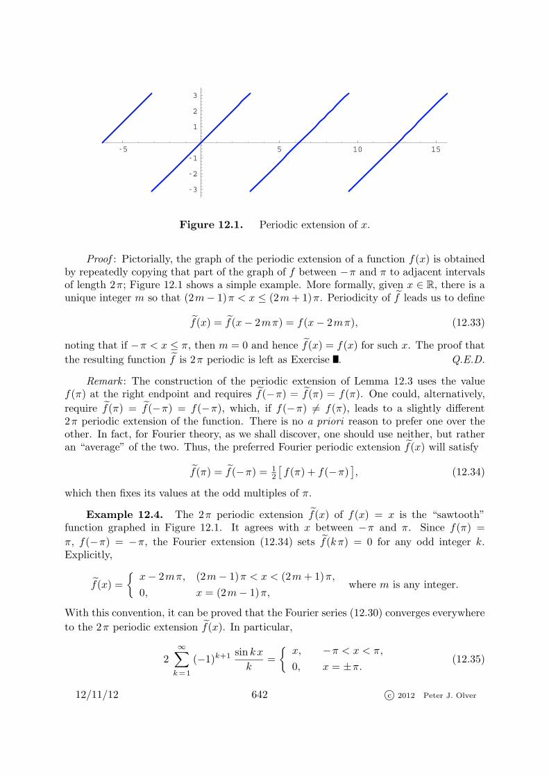
Figure 12.1. Periodic extension of x.

Proof : Pictorially, the graph of the periodic extension of a function f(x) is obtainedby repeatedly copying that part of the graph of f between −π and π to adjacent intervalsof length 2π; Figure 12.1 shows a simple example. More formally, given x ∈ R, there is aunique integer m so that (2m− 1)π < x ≤ (2m+ 1)π. Periodicity of �f leads us to define

�f(x) = �f(x− 2mπ) = f(x− 2mπ), (12.33)

noting that if −π < x ≤ π, then m = 0 and hence �f(x) = f(x) for such x. The proof that

the resulting function �f is 2π periodic is left as Exercise . Q.E.D.

Remark : The construction of the periodic extension of Lemma 12.3 uses the valuef(π) at the right endpoint and requires �f(−π) = �f(π) = f(π). One could, alternatively,

require �f(π) = �f(−π) = f(−π), which, if f(−π) �= f(π), leads to a slightly different2π periodic extension of the function. There is no a priori reason to prefer one over theother. In fact, for Fourier theory, as we shall discover, one should use neither, but ratheran “average” of the two. Thus, the preferred Fourier periodic extension �f(x) will satisfy

�f(π) = �f(−π) = 12

�f(π) + f(−π)

�, (12.34)

which then fixes its values at the odd multiples of π.

Example 12.4. The 2π periodic extension �f(x) of f(x) = x is the “sawtooth”function graphed in Figure 12.1. It agrees with x between −π and π. Since f(π) =

π, f(−π) = −π, the Fourier extension (12.34) sets �f(kπ) = 0 for any odd integer k.Explicitly,

�f(x) =�

x− 2mπ, (2m− 1)π < x < (2m+ 1)π,

0, x = (2m− 1)π,where m is any integer.

With this convention, it can be proved that the Fourier series (12.30) converges everywhere

to the 2π periodic extension �f(x). In particular,

2∞�

k=1

(−1)k+1 sin kx

k=

�x, −π < x < π,

0, x = ±π.(12.35)

12/11/12 642 c� 2012 Peter J. Olver

Even this very simple example has remarkable and nontrivial consequences. For in-stance, if we substitute x = 1

2π in (12.30) and divide by 2, we obtain Gregory’s series

π

4= 1 − 1

3+

1

5− 1

7+

1

9− · · · . (12.36)

While this striking formula predates Fourier theory — it was, in fact, first discovered byLeibniz — a direct proof is not easy.

Remark : While numerologically fascinating, Gregory’s series is of scant practical usefor actually computing π since its rate of convergence is painfully slow. The reader maywish to try adding up terms to see how far out one needs to go to accurately computeeven the first two decimal digits of π. Round-off errors will eventually interfere with anyattempt to compute the complete summation to any reasonable degree of accuracy.

Piecewise Continuous Functions

As we shall see, all continuously differentiable, 2π periodic functions can be repre-sented as convergent Fourier series. More generally, we can allow the function to havesome simple discontinuities. Although not the most general class of functions that pos-sess convergent Fourier series, such “piecewise continuous” functions will suffice for all theapplications we consider in this text.

Definition 12.5. A function f(x) is said to be piecewise continuous on an interval[a, b ] if it is defined and continuous except possibly at a finite number of points a ≤ x1 <x2 < . . . < xn ≤ b. At each point of discontinuity, the left and right hand limits†

f(x−k ) = lim

x→ x−

k

f(x), f(x+k ) = lim

x→ x+

k

f(x),

exist. Note that we do not require that f(x) be defined at xk. Even if f(xk) is defined, itdoes not necessarily equal either the left or the right hand limit.

A function f(x) defined for all x ∈ R is piecewise continuous provided it is piece-

wise continuous on every bounded interval. In particular, a 2π periodic function �f(x) ispiecewise continuous if and only if it is piecewise continuous on the interval [−π, π ].

A representative graph of a piecewise continuous function appears in Figure 12.2. Thepoints xk are known as jump discontinuities of f(x) and the difference

βk = f(x+k )− f(x−

k ) = limx→ x+

k

f(x)− limx→ x−

k

f(x) (12.37)

between the left and right hand limits is the magnitude of the jump, cf. (11.49). If βk = 0,and so the right and left hand limits agree, then the discontinuity is removable sinceredefining f(xk) = f(x+

k ) = f(x−k ) makes f continuous at xk. We will assume, without

significant loss of generality, that our functions have no removable discontinuities.

† At the endpoints a, b we only require one of the limits, namely f(a+) and f(b−), to exist.

12/11/12 643 c� 2012 Peter J. Olver

-1 1 2 3 4

-1

-0.5

0.5

1

Figure 12.2. Piecewise Continuous Function.

The simplest example of a piecewise continuous function is the step function

σ(x) =

�1, x > 0,

0, x < 0.(12.38)

It has a single jump discontinuity at x = 0 of magnitude 1, and is continuous — indeed,constant — everywhere else. If we translate and scale the step function, we obtain afunction

h(x) = β σ(x− y) =

�β, x > y,

0, x < y,(12.39)

with a single jump discontinuity of magnitude β at the point x = y.

If f(x) is any piecewise continuous function, then its Fourier coefficients are well-defined — the integrals (12.28) exist and are finite. Continuity, however, is not enough toensure convergence of the resulting Fourier series.

Definition 12.6. A function f(x) is called piecewise C1 on an interval [a, b ] if it isdefined, continuous and continuously differentiable except possibly at a finite number ofpoints a ≤ x1 < x2 < . . . < xn ≤ b. At each exceptional point, the left and right handlimits† exist:

f(x−k ) = lim

x→x−

k

f(x), f(x+k ) = lim

x→x+

k

f(x),

f ′(x−k ) = lim

x→x−

k

f ′(x), f ′(x+k ) = lim

x→x+

k

f ′(x).

See Figure 12.3 for a representative graph. For a piecewise continuous C1 function,an exceptional point xk is either

• a jump discontinuity of f , but where the left and right hand derivatives exist, or

• a corner , meaning a point where f is continuous, so f(x−k ) = f(x+

k ), but has differentleft and right hand derivatives: f ′(x−

k ) �= f ′(x+k ).

† As before, at the endpoints we only require the appropriate one-sided limits, namely f(a+),

f ′(a+) and f(b−), f ′(b−), to exist.

12/11/12 644 c� 2012 Peter J. Olver

-1 1 2 3 4

-1

-0.5

0.5

1

Figure 12.3. Piecewise C1 Function.

Thus, at each point, including jump discontinuities, the graph of f(x) has well-definedright and left tangent lines. For example, the function f(x) = | x | is piecewise C1 since itis continuous everywhere and has a corner at x = 0, with f ′(0+) = +1, f ′(0−) = −1.

There is an analogous definition of a piecewise Cn function. One requires that thefunction has n continuous derivatives, except at a finite number of points. Moreover, atevery point, the function has well-defined right and left hand limits of all its derivativesup to order n.

The Convergence Theorem

We are now able to state the fundamental convergence theorem for Fourier series.

Theorem 12.7. If �f(x) is any 2π periodic, piecewise C1 function, then, for any

x ∈ R, its Fourier series converges to

�f(x), if �f is continuous at x,12

� �f(x+) + �f(x−)�, if x is a jump discontinuity.

Thus, the Fourier series converges, as expected, to �f(x) at all points of continuity;at discontinuities, the Fourier series can’t decide whether to converge to the right or lefthand limit, and so ends up “splitting the difference” by converging to their average; seeFigure 12.4. If we redefine �f(x) at its jump discontinuities to have the average limitingvalue, so

�f(x) = 12

� �f(x+) + �f(x−)�, (12.40)

— an equation that automatically holds at all points of continuity — then Theorem 12.7

would say that the Fourier series converges to �f(x) everywhere. We will discuss the ideasunderlying the proof of the Convergence Theorem 12.7 at the end of Section 12.5.

Example 12.8. Let σ(x) denote the step function (12.38). Its Fourier coefficients

12/11/12 645 c� 2012 Peter J. Olver

Figure 12.4. Splitting the Difference.

are easily computed:

a0 =1

π

� π

−π

σ(x) dx =1

π

� π

0

dx = 1,

ak =1

π

� π

−π

σ(x) cos kx dx =1

π

� π

0

cos kx dx = 0,

bk =1

π

� π

−π

σ(x) sin kx dx =1

π

� π

0

sin kx dx =

2

kπ, k = 2 l + 1 odd,

0, k = 2 l even.

Therefore, the Fourier series for the step function is

σ(x) ∼ 1

2+

2

π

�sinx +

sin 3x

3+

sin 5x

5+

sin 7x

7+ · · ·

�. (12.41)

According to Theorem 12.7, the Fourier series will converge to the 2π periodic extensionof the step function:

�σ(x) =

0, (2m− 1)π < x < 2mπ,

1, 2mπ < x < (2m+ 1)π,12 , x = mπ,

where m is any integer,

which is plotted in Figure 12.5. Observe that, in accordance with Theorem 12.7, �σ(x)takes the midpoint value 1

2 at the jump discontinuities 0,±π,±2π, . . . .

It is instructive to investigate the convergence of this particular Fourier series insome detail. Figure 12.6 displays a graph of the first few partial sums, taking, respectively,n = 3, 5, and 10 terms. The reader will notice that away from the discontinuities, the seriesdoes appear to be converging, albeit slowly. However, near the jumps there is a consistentovershoot of about 9%. The region where the overshoot occurs becomes narrower andnarrower as the number of terms increases, but the magnitude of the overshoot persists nomatter how many terms are summed up. This was first noted by the American physicistJosiah Gibbs, and is now known as the Gibbs phenomenon in his honor. The Gibbsovershoot is a manifestation of the subtle non-uniform convergence of the Fourier series.

12/11/12 646 c� 2012 Peter J. Olver

-5 5 10 15

-1

-0.5

0.5

1

Figure 12.5. Periodic Step Function.

-3 -2 -1 1 2 3

-1

-0.5

0.5

1

-3 -2 -1 1 2 3

-1

-0.5

0.5

1

-3 -2 -1 1 2 3

-1

-0.5

0.5

1

Figure 12.6. Gibbs Phenomenon.

Even and Odd Functions

We already noted that the Fourier cosine coefficients of the function f(x) = x are all0. This is not an accident, but rather a direct consequence of the fact that x is an oddfunction. Recall first the basic definition:

Definition 12.9. A function is called even if f(−x) = f(x). A function is odd iff(−x) = −f(x).

For example, the functions 1, cos kx, and x2 are all even, whereas x, sin kx, and signxare odd. We require two elementary lemmas, whose proofs are left to the reader.

Lemma 12.10. The sum, f(x)+ g(x), of two even functions is even; the sum of two

odd functions is odd. The product f(x) g(x) of two even functions, or of two odd functions,

is an even function. The product of an even and an odd function is odd.

Remark : Every function can be represented as the sum of an even and an odd function;see Exercise .

12/11/12 647 c� 2012 Peter J. Olver

Lemma 12.11. If f(x) is odd and integrable on the symmetric interval [−a, a ], then� a

−a

f(x) dx = 0. If f(x) is even and integrable, then

� a

−a

f(x)dx = 2

� a

0

f(x)dx.

The next result is an immediate consequence of applying Lemmas 12.10 and 12.11 tothe Fourier integrals (12.28).

Proposition 12.12. If f(x) is even, then its Fourier sine coefficients all vanish,

bk = 0, and so f can be represented by a Fourier cosine series

f(x) ∼ a02

+∞�

k=1

ak cos kx , (12.42)

where

ak =2

π

� π

0

f(x) coskx dx, k = 0, 1, 2, 3, . . . . (12.43)

If f(x) is odd, then its Fourier cosine coefficients vanish, ak = 0, and so f can be represented

by a Fourier sine series

f(x) ∼∞�

k=1

bk sin kx , (12.44)

where

bk =2

π

� π

0

f(x) sin kx dx, k = 1, 2, 3, . . . . (12.45)

Conversely, a convergent Fourier cosine (respectively, sine) series always represents an even

(respectively, odd) function.

Example 12.13. The absolute value f(x) = | x | is an even function, and hence hasa Fourier cosine series. The coefficients are

a0 =2

π

� π

0

x dx = π, (12.46)

ak =2

π

� π

0

x cos kx dx =2

π

�x sin kx

k+

cos kx

k2

�π

x=0

=

0, 0 �= k even,

− 4

k2π, k odd.

Therefore

| x | ∼ π

2− 4

π

�cosx +

cos 3x

9+

cos 5x

25+

cos 7x

49+ · · ·

�. (12.47)

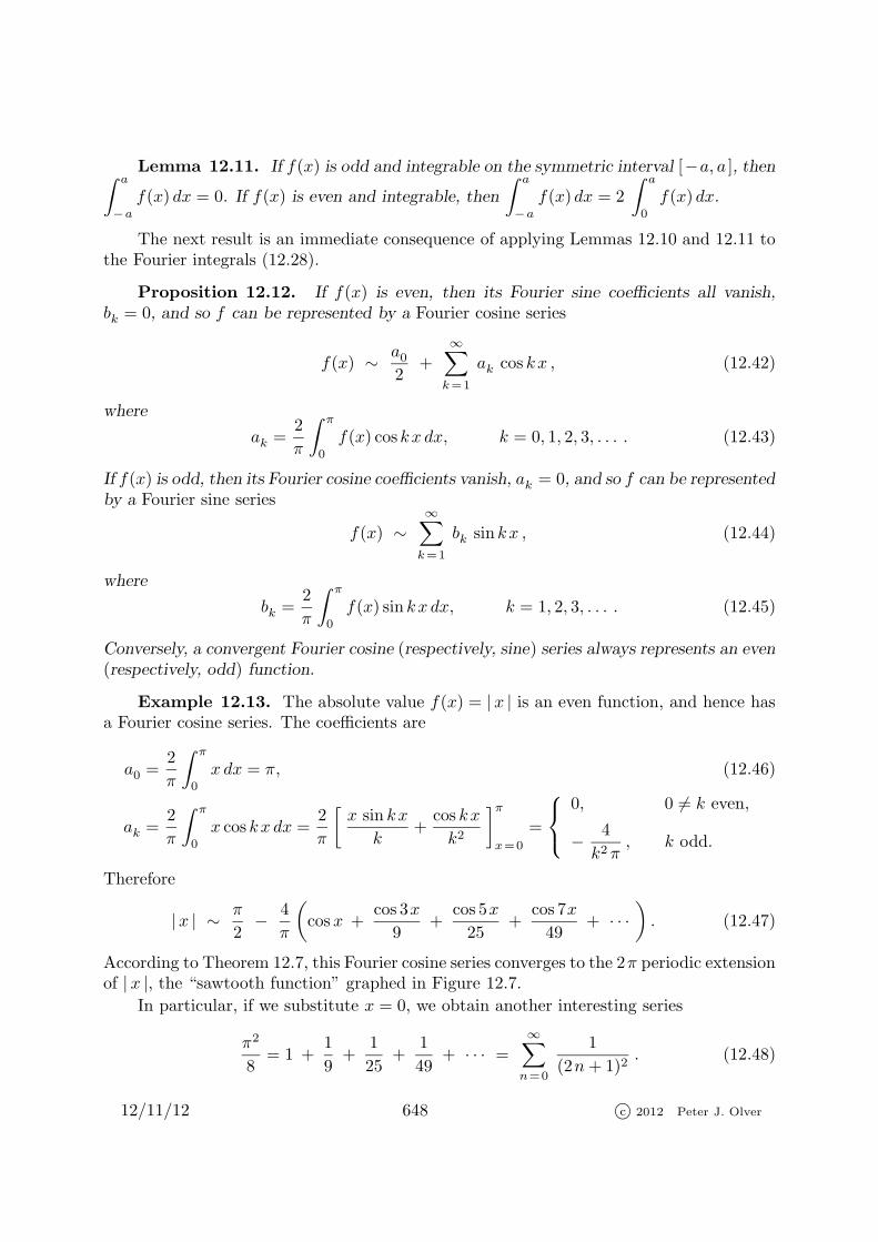
According to Theorem 12.7, this Fourier cosine series converges to the 2π periodic extensionof | x |, the “sawtooth function” graphed in Figure 12.7.

In particular, if we substitute x = 0, we obtain another interesting series

π2

8= 1 +

1

9+

1

25+

1

49+ · · · =

∞�

n=0

1

(2n+ 1)2. (12.48)

12/11/12 648 c� 2012 Peter J. Olver

-5 5 10 15

-3

-2

-1

1

2

3

Figure 12.7. Periodic extension of | x |.

It converges faster than Gregory’s series (12.36), and, while far from optimal in this regards,can be used to compute reasonable approximations to π. One can further manipulate thisresult to compute the sum of the series

S =∞�

n=1

1

n2= 1 +

1

4+

1

9+

1

16+

1

25+

1

36+

1

49+ · · · .

We note that

S

4=

∞�

n=1

1

4n2=

∞�

n=1

1

(2n)2=

1

4+

1

16+

1

36+

1

64+ · · · .

Therefore, by (12.48),

3

4S = S − S

4= 1 +

1

9+

1

25+

1

49+ · · · =

π2

8,

from which we conclude that

S =∞�

n=1

1

n2= 1 +

1

4+

1

9+

1

16+

1

25+ · · · =

π2

6. (12.49)

Remark : The most famous function in number theory — and the source of the mostoutstanding problem in mathematics, the Riemann hypothesis — is the Riemann zeta

function

ζ(s) =∞�

n=1

1

ns. (12.50)

Formula (12.49) shows that ζ(2) = 16 π

2. In fact, the value of the zeta function at any even

positive integer s = 2n can be written as a rational polynomial in π.

If f(x) is any function defined on [0, π ], then its Fourier cosine series is defined bythe formulas (12.42–43); the resulting series represents its even, 2π periodic extension. Forexample, the cosine series of f(x) = x is given in (12.47); indeed the even, 2π periodic

12/11/12 649 c� 2012 Peter J. Olver

extension of x coincides with the 2π periodic extension of | x |. Similarly, the formulas(12.44, 45) define its Fourier sine series , representing its odd, 2π periodic extension. Inparticular, since f(x) = x is already odd, its Fourier sine series concides with its ordinaryFourier series.

Complex Fourier Series

An alternative, and often more convenient, approach to Fourier series is to use complexexponentials instead of sines and cosines. Indeed, Euler’s formula

e i kx = cos kx+ i sin kx, e− i kx = cos kx− i sin kx, (12.51)

shows how to write the trigonometric functions

cos kx =e i kx + e− i kx

2, sin kx =

e i kx − e− i kx

2 i, (12.52)

in terms of complex exponentials. Orthonormality with respect to the rescaled L2 Hermi-tian inner product

� f ; g � = 1

2π

� π

−π

f(x) g(x)dx , (12.53)

was proved by direct computation in Example 3.45:

� e i kx ; e i lx � = 1

2π

� π

−π

e i (k−l)x dx =

�1, k = l,

0, k �= l,

� e i kx �2 =1

2π

� π

−π

| e i kx |2 dx = 1.

(12.54)

Again, orthogonality follows from their status as (complex) eigenfunctions for the periodicboundary value problem (12.13).

The complex Fourier series for a (piecewise continuous) real or complex function f is

f(x) ∼∞�

k=−∞ck e

i kx = · · · +c−2 e−2 ix+c−1 e

− ix+c0+c1 eix+c2 e

2 ix+ · · · . (12.55)

The orthonormality formulae (12.53) imply that the complex Fourier coefficients are ob-tained by taking the inner products

ck = � f ; e i kx � = 1

2π

� π

−π

f(x) e− i kx dx (12.56)

with the associated complex exponential. Pay attention to the minus sign in the integratedexponential — the result of taking the complex conjugate of the second argument in theinner product (12.53). It should be emphasized that the real (12.27) and complex (12.55)Fourier formulae are just two different ways of writing the same series! Indeed, if we apply

12/11/12 650 c� 2012 Peter J. Olver

Euler’s formula (12.51) to (12.56) and compare with the real Fourier formulae (12.28), wefind that the real and complex Fourier coefficients are related by

ak = ck + c−k,

bk = i (ck − c−k),

ck = 12 (ak − i bk),

c−k = 12 (ak + i bk),

k = 0, 1, 2, . . . . (12.57)

Remark : We already see one advantage of the complex version. The constant function1 = e0 i x no longer plays an anomalous role — the annoying factor of 1

2 in the real Fourierseries (12.27) has mysteriously disappeared!

Example 12.14. For the step function σ(x) considered in Example 12.8, the complexFourier coefficients are

ck =1

2π

� π

−π

σ(x) e− i kx dx =1

2π

� π

0

e− i kx dx =

12 , k = 0,

0, 0 �= k even,

1

i k π, k odd.

Therefore, the step function has the complex Fourier series

σ(x) ∼ 1

2− i

π

∞�

l=−∞

e(2 l+1) ix

2 l + 1.

You should convince yourself that this is exactly the same series as the real Fourier series(12.41). We are merely rewriting it using complex exponentials instead of real sines andcosines.

Example 12.15. Let us find the Fourier series for the exponential function eax. Itis much easier to evaluate the integrals for the complex Fourier coefficients, and so

ck = � eax ; e ikx � = 1

2π

� π

−π

e(a− i k)x dx =e(a− i k)x

2π (a− i k)

����π

x=−π

=e(a− i k)π − e−(a− i k)π

2π (a− i k)= (−1)k

eaπ − e−aπ

2π (a− i k)=

(−1)k(a+ i k) sinh aπ

π (a2 + k2).

Therefore, the desired Fourier series is

eax ∼ sinh aπ

π

∞�

k=−∞

(−1)k(a+ i k)

a2 + k2e i kx. (12.58)

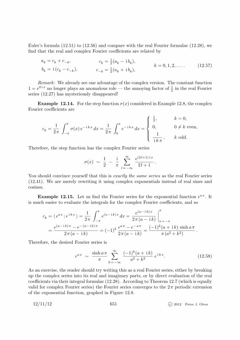
As an exercise, the reader should try writing this as a real Fourier series, either by breakingup the complex series into its real and imaginary parts, or by direct evaluation of the realcoefficients via their integral formulae (12.28). According to Theorem 12.7 (which is equallyvalid for complex Fourier series) the Fourier series converges to the 2π periodic extensionof the exponential function, graphed in Figure 12.8.

12/11/12 651 c� 2012 Peter J. Olver

-5 5 10 15

5

10

15

20

Figure 12.8. Periodic Extension of ex.

The Delta Function

Fourier series can even be used to represent more general objects than mere functions.The most important example is the delta function δ(x). Using its characterizing properties(11.37), the real Fourier coefficients are computed as

ak =1

π

� π

−π

δ(x) cos kx dx =1

πcos k0 =

1

π,

bk =1

π

� π

−π

δ(x) sin kx dx =1

πsin k0 = 0.

(12.59)

Therefore,

δ(x) ∼ 1

2π+

1

π

�cosx+ cos 2x+ cos 3x+ · · ·

�. (12.60)

Since δ(x) is an even function, it should come as no surprise that it has a cosine series.

To understand in what sense this series converges to the delta function, it will help torewrite it in complex form

δ(x) ∼ 1

2π

∞�

k=−∞e i kx =

1

2π

�· · · + e−2 ix + e− ix + 1 + e ix + e2 ix + · · ·

�. (12.61)

where the complex Fourier coefficients are computed† as

ck =1

2π

� π

−π

δ(x) e− i kx dx =1

2π.

† Or, we could use (12.57).

12/11/12 652 c� 2012 Peter J. Olver

Figure 12.9. Partial Fourier Sums Approximating the Delta Function.

The nth partial sum

sn(x) =1

2π

n�

k=−n

e i kx =1

2π

�e− inx + · · · + e− ix + 1 + e ix + · · · + e inx

�

can, in fact, be explicitly evaluated. Recall the formula for the sum of a geometric series

m�

k=0

a rk = a+ a r + a r2 + · · · + a rm = a

�rm+1 − 1

r − 1

�. (12.62)

The partial sum sn(x) has this form, withm+1 = 2n+1 summands, initial term a = e− inx,and ratio r = e ix. Therefore,

sn(x) =1

2π

n�

k=−n

e i kx =1

2πe− inx

�e i (2n+1)x − 1

e ix − 1

�=

1

2π

e i (n+1)x − e− inx

e ix − 1

=1

2π

e i�n+

12

�x − e− i

�n+

12

�x

e ix/2 − e− ix/2=

1

2π

sin�n+ 1

2

�x

sin 12x

.

(12.63)

In this computation, to pass from the first to the second line, we multiplied numeratorand denominator by e− i x/2, after which we used the formula (3.86) for the sine functionin terms of complex exponentials. Incidentally, (12.63) is equivalent to the intriguingtrigonometric summation formula

sn(x) =1

2π+

1

π

�cosx+ cos 2x+ cos 3x+ · · · + cosnx

�=

1

2π

sin�n+ 1

2

�x

sin 12 x

. (12.64)

Graphs of the partial sums sn(x) for several values of n are displayed in Figure 12.9.Note that the spike, at x = 0, progressively becomes taller and thinner, converging to an

12/11/12 653 c� 2012 Peter J. Olver

infinitely tall, infinitely thin delta spike. Indeed, by l’Hopital’s Rule,

limx→0

1

2π

sin�n+ 1

2

�x

sin 12x

= limx→0

1

2π

�n+ 1

2

�cos

�n+ 1

2

�x

12cos 1

2x

=n+ 1

2

π−→ ∞ as n → ∞.

(An elementary proof of this formula is to note that, at x = 0, every term in the originalsum (12.64) is equal to 1.) Furthermore, the integrals remain fixed,

1

2π

� π

−π

sn(x) dx =1

2π

� π

−π

sin�n+ 1

2

�x

sin 12 x

dx =1

2π

� π

−π

n�

k=−n

e i kx dx = 1, (12.65)

as required for convergence to the delta function. However, away from the spike, the partialsums do not go to zero! Rather, they oscillate more and more rapidly, maintaining anoverall amplitude of 1

2π csc 12 x = 1/

�2π sin 1

2 x�. As n gets large, the amplitude function

appears as an envelope of the increasingly rapid oscillations. Roughly speaking, the factthat sn(x) → δ(x) as n → ∞ means that the “infinitely fast” oscillations somehow canceleach other out, and the net effect is zero away from the spike at x = 0. Thus, theconvergence of the Fourier sums to δ(x) is much more subtle than in the original limitingdefinition (11.31). The technical term is weak convergence, which plays an very importantrole in advanced mathematical analysis, [159]; see Exercise below for additional details.

Remark : Although we stated that the Fourier series (12.60, 61) represent the deltafunction, this is not entirely correct. Remember that a Fourier series converges to the2π periodic extension of the original function. Therefore, (12.61) actually represents theperiodic extension of the delta function:

�δ(x) = · · · +δ(x+4π)+δ(x+2π)+δ(x)+δ(x−2π)+δ(x−4π)+δ(x−6π)+ · · · , (12.66)

consisting of a periodic array of delta spikes concentrated at all integer multiples of 2π.

12.3. Differentiation and Integration.

If a series of functions converges “nicely” then one expects to be able to integrateand differentiate it term by term; the resulting series should converge to the integral andderivative of the original sum. Integration and differentiation of power series is alwaysvalid within the range of convergence, and is used extensively in the construction of seriessolutions of differential equations, series for integrals of non-elementary functions, and soon. The interested reader can consult Appendix C for further details.

As we now appreciate, the convergence of Fourier series is a much more delicate mat-ter, and so one must be considerably more careful with their differentiation and integration.Nevertheless, in favorable situations, both operations lead to valid results, and are quiteuseful for constructing Fourier series of more complicated functions. It is a remarkable,profound fact that Fourier analysis is completely compatible with the calculus of general-ized functions that we developed in Chapter 11. For instance, differentiating the Fourierseries for a piecewise C1 function leads to the Fourier series for the differentiated functionthat has delta functions of the appropriate magnitude appearing at each jump discontinu-ity. This fact reassures us that the rather mysterious construction of delta functions and

12/11/12 654 c� 2012 Peter J. Olver

their generalizations is indeed the right way to extend calculus to functions which do notpossess derivatives in the ordinary sense.

Integration of Fourier Series

Integration is a smoothing operation — the integrated function is always nicer thanthe original. Therefore, we should anticipate being able to integrate Fourier series withoutdifficulty. There is, however, one complication: the integral of a periodic function is notnecessarily periodic. The simplest example is the constant function 1, which is certainlyperiodic, but its integral, namely x, is not. On the other hand, integrals of all the otherperiodic sine and cosine functions appearing in the Fourier series are periodic. Thus, onlythe constant term might cause us difficulty when we try to integrate a Fourier series (12.27).According to (2.4), the constant term

a02

=1

2π

� π

−π

f(x) dx (12.67)

is the mean or average of the function f(x) on the interval [−π, π ]. A function has noconstant term in its Fourier series if and only if it has mean zero. It is easily shown,cf. Exercise , that the mean zero functions are precisely the ones that remain periodicupon integration.

Lemma 12.16. If f(x) is 2π periodic, then its integral g(x) =

� x

0

f(y)dy is 2π

periodic if and only if

� π

−π

f(x) dx = 0, so that f has mean zero on the interval [−π, π ].

In particular, Lemma 12.11 implies that all odd functions automatically have meanzero, and hence periodic integrals.

Since �cos kx dx =

sin kx

k,

�sin kx dx = − cos kx

k, (12.68)

termwise integration of a Fourier series without constant term is straightforward. Theresulting Fourier series is given precisely as follows.

Theorem 12.17. If f is piecewise continuous, 2π periodic, and has mean zero, then

its Fourier series

f(x) ∼∞�

k=1

[ ak cos kx+ bk sin kx ] ,

can be integrated term by term, to produce the Fourier series

g(x) =

� x

0

f(y)dy ∼ m +∞�

k=1

�− bk

kcos kx+

akk

sin kx

�, (12.69)

for its periodic integral. The constant term

m =1

2π

� π

−π

g(x)dx (12.70)

is the mean of the integrated function.

12/11/12 655 c� 2012 Peter J. Olver

In many situations, the integration formula (12.69) provides a very convenient alter-native to the direct derivation of the Fourier coefficients.

Example 12.18. The function f(x) = x is odd, and so has mean zero:

� π

−π

x dx = 0.Let us integrate its Fourier series

x ∼ 2

∞�

k=1

(−1)k−1

ksin kx (12.71)

that we found in Example 12.2. The result is the Fourier series

1

2x2 ∼ π2

6− 2

∞�

k=1

(−1)k−1

k2cos kx

=π2

6− 2

�cosx − cos 2x

4+

cos 3x

9− cos 4x

16+ · · ·

�,

(12.72)

whose the constant term is the mean of the left hand side:

1

2π

� π

−π

x2

2dx =

π2

6.

Let us revisit the derivation of the integrated Fourier series from a slightly differentstandpoint. If we were to integrate each trigonometric summand in a Fourier series (12.27)from 0 to x, we would obtain

� x

0

cos ky dy =sin kx

k, whereas

� x

0

sin ky dy =1

k− cos kx

k.

The extra 1/k terms arising from the definite sine integrals do not appear explicitly inour previous form for the integrated Fourier series, (12.69), and so must be hidden inthe constant term m. We deduce that the mean value of the integrated function can becomputed using the Fourier sine coefficients of f via the formula

1

2π

� π

−π

g(x)dx = m =∞�

k=1

bkk. (12.73)

For example, the result of integrating both sides of the Fourier series (12.71) for f(x) = xfrom 0 to x is

x2

2∼ 2

∞�

k=1

(−1)k−1

k2(1− cos kx).

The constant terms sum up to yield the mean value of the integrated function:

2

�1− 1

4+

1

9− 1

16+ . . .

�= 2

∞�

k=1

(−1)k−1

k2=

1

2π

� π

−π

x2

2dx =

π2

6, (12.74)

which reproduces a formula established in Exercise .

12/11/12 656 c� 2012 Peter J. Olver

More generally, if f(x) does not have mean zero, its Fourier series has a nonzeroconstant term,

f(x) ∼ a02

+∞�

k=1

[ ak cos kx+ bk sin kx ] .

In this case, the result of integration will be

g(x) =

� x

0

f(y)dy ∼ a02

x+m+

∞�

k=1

�− bk

kcos kx+

akk

sin kx

�, (12.75)

where m is given in (12.73). The right hand side is not, strictly speaking, a Fourier series.There are two ways to interpret this formula within the Fourier framework. Either we canwrite (12.75) as the Fourier series for the difference

g(x)− a02

x ∼ m+

∞�

k=1

�− bk

kcos kx+

akk

sin kx

�, (12.76)

which is a 2π periodic function, cf. Exercise . Alternatively, one can replace x by itsFourier series (12.30), and the result will be the Fourier series for the 2π periodic extension

of the integral g(x) =

� x

0

f(y)dy.

Differentiation of Fourier Series

Differentiation has the opposite effect to integration. Differentiation makes a functionworse. Therefore, to justify taking the derivative of a Fourier series, we need to know thatthe differentiated function remains reasonably nice. Since we need the derivative f ′(x) tobe piecewise C1 for the convergence Theorem 12.7 to be applicable, we must require thatf(x) itself be continuous and piecewise C2.

Theorem 12.19. If f is 2π periodic, continuous, and piecewise C2, then its Fourier

series can be differentiated term by term, to produce the Fourier series for its derivative

f ′(x) ∼∞�

k=1

�k bk cos kx− k ak sin kx

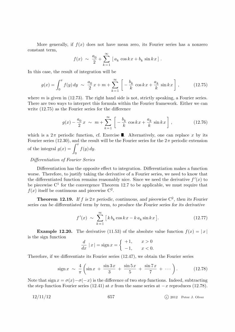
�. (12.77)

Example 12.20. The derivative (11.53) of the absolute value function f(x) = | x |is the sign function

d

dx| x | = signx =

�+1, x > 0

−1, x < 0.

Therefore, if we differentiate its Fourier series (12.47), we obtain the Fourier series

signx ∼ 4

π

�sinx +

sin 3x

3+

sin 5x

5+

sin 7x

7+ · · ·

�. (12.78)

Note that signx = σ(x)−σ(−x) is the difference of two step functions. Indeed, subtractingthe step function Fourier series (12.41) at x from the same series at −x reproduces (12.78).

12/11/12 657 c� 2012 Peter J. Olver

Example 12.21. If we differentiate the Fourier series

x ∼ 2∞�

k=1

(−1)k−1

ksin kx = 2

�sinx − sin 2x

2+

sin 3x

3− sin 4x

4+ · · ·

�,

we obtain an apparent contradiction:

1 ∼ 2∞�

k=1

(−1)k+1 cos kx = 2 cosx− 2 cos 2x+ 2 cos 3x− 2 cos 4x+ · · · . (12.79)

But the Fourier series for 1 just consists of a single constant term! (Why?)

The resolution of this paradox is not difficult. The Fourier series (12.30) does not

converge to x, but rather to its periodic extension �f(x), which has a jump discontinuity ofmagnitude 2π at odd multiples of π; see Figure 12.1. Thus, Theorem 12.19 is not directlyapplicable. Nevertheless, we can assign a consistent interpretation to the differentiatedseries. The derivative �f ′(x) of the periodic extension is not equal to the constant function1, but, rather, has an additional delta function concentrated at each jump discontinuity:

�f ′(x) = 1− 2π

∞�

j=−∞δ�x− (2j + 1)π

�= 1− 2π �δ(x− π),

where �δ denotes the 2π periodic extension of the delta function, cf. (12.66). The dif-ferentiated Fourier series (12.79) does, in fact, converge to this modified distributionalderivative! Indeed, differentiation and integration of Fourier series is entirely compatiblewith the calculus of generalized functions, as will be borne out in yet another example.

Example 12.22. Let us differentiate the Fourier series (12.41) for the step functionand see if we end up with the Fourier series (12.60) for the delta function. We find

d

dxσ(x) ∼ 2

π

�cosx+ cos 3x+ cos 5x+ cos 7x+ · · ·

�, (12.80)

which does not agree with (12.60) — half the terms are missing! The explanation issimilar to the preceding example: the 2π periodic extension of the step function has twojump discontinuities, of magnitudes +1 at even multiples of π and −1 at odd multiples.Therefore, its derivative is the difference of the 2π periodic extension of the delta functionat 0, with Fourier series (12.60) minus the 2π periodic extension of the delta function atπ, with Fourier series

δ(x− π) ∼ 1

2π+

1

π

�− cosx+ cos 2x− cos 3x+ · · ·

�

derived in Exercise . The difference of these two delta function series produces (12.80).

12.4. Change of Scale.

So far, we have only dealt with Fourier series on the standard interval of length 2π.(We chose [−π, π ] for convenience, but all of the results and formulas are easily adapted

12/11/12 658 c� 2012 Peter J. Olver

to any other interval of the same length, e.g., [0, 2π ].) Since physical objects like bars andstrings do not all come in this particular length, we need to understand how to adapt theformulas to more general intervals. The basic idea is to rescale the variable so as to stretchor contract the standard interval†.

Any symmetric interval [−ℓ , ℓ ] of length 2 ℓ can be rescaled to the standard interval[−π, π ] by using the linear change of variables

x =ℓ

πy, so that − π ≤ y ≤ π whenever − ℓ ≤ x ≤ ℓ. (12.81)

Given a function f(x) defined on [−ℓ , ℓ ], the rescaled function F (y) = f

�ℓ

πy

�lives on

[−π, π ]. Let

F (y) ∼ a02

+∞�

k=1

�ak cos ky + bk sin ky

�,

be the standard Fourier series for F (y), so that

ak =1

π

� π

−π

F (y) cosky dy, bk =1

π

� π

−π

F (y) sin ky dy. (12.82)

Then, reverting to the unscaled variable x, we deduce that

f(x) ∼ a02

+

∞�

k=1

�ak cos

kπx

ℓ+ bk sin

kπx

ℓ

�. (12.83)

The Fourier coefficients ak, bk can be computed directly from f(x). Indeed, replacing theintegration variable in (12.82) by y = πx/ℓ, and noting that dy = (π/ℓ ) dx, we deduce theadapted formulae

ak =1

ℓ

� ℓ

−ℓ

f(x) coskπx

ℓdx, bk =

1

ℓ

� ℓ

−ℓ

f(x) sinkπx

ℓdx, (12.84)

for the Fourier coefficients of f(x) on the interval [−ℓ , ℓ ].

All of the convergence results, integration and differentiation formulae, etc., thatare valid for the interval [−π, π ] carry over, essentially unchanged, to Fourier series onnonstandard intervals. In particular, adapting our basic convergence Theorem 12.7, weconclude that if f(x) is piecewise C1, then its rescaled Fourier series (12.83) converges

to its 2 ℓ periodic extension �f(x), subject to the proviso that �f(x) takes on the midpointvalues at all jump discontinuities.

Example 12.23. Let us compute the Fourier series for the function f(x) = x on theinterval −1 ≤ x ≤ 1. Since f is odd, only the sine coefficients will be nonzero. We have

bk =

� 1

−1

x sin kπxdx =

�− x cos kπx

kπ+

sin kπx

(kπ)2

�1

x=−1

=2(−1)k+1

k π.

† The same device was already used, in Section 5.4, to adapt the orthogonal Legendre polyno-mials to other intervals.

12/11/12 659 c� 2012 Peter J. Olver

-4 -2 2 4 6

-1

-0.5

0.5

1

Figure 12.10. 2 Periodic Extension of x.

The resulting Fourier series is

x ∼ 2

π

�sinπx − sin 2πx

2+

sin 3πx

3− · · ·

�.

The series converges to the 2 periodic extension of the function x, namely

�f(x) =�

x− 2m, 2m− 1 < x < 2m+ 1,

0, x = m,where m is an arbitrary integer,

plotted in Figure 12.10.

We can similarly reformulate complex Fourier series on the nonstandard interval[−ℓ , ℓ ]. Using (12.81) to rescale the variables in (12.55), we find

f(x) ∼∞�

k=−∞ck e

i kπx/ℓ, where ck =1

2 ℓ

� ℓ

−ℓ

f(x) e− i kπx/ℓ dx. (12.85)

Again, this is merely an alternative way of writing the real Fourier series (12.83).

When dealing with a more general interval [a, b ], there are two options. The first is to

take a function f(x) defined for a ≤ x ≤ b and periodically extend it to a function �f(x) thatagrees with f(x) on [a, b ] and has period b− a. One can then compute the Fourier series

(12.83) for its periodic extension �f(x) on the symmetric interval [ 12(a−b), 12(b−a) ] of width

2 ℓ = b − a; the resulting Fourier series will (under the appropriate hypotheses) convergeto �f(x) and hence agree with f(x) on the original interval. An alternative approach is totranslate the interval by an amount 1

2 (a+b) so as to make it symmetric; this is accomplishedby the change of variables �x = x− 1

2(a+b). an additional rescaling will convert the interval

into [−π, π ]. The two methods are essentially equivalent, and full details are left to thereader.

12.5. Convergence of the Fourier Series.

The purpose of this final section is to establish some basic convergence results forFourier series. This is not a purely theoretical exercise, since convergence considerationsimpinge directly upon a variety of applications of Fourier series. One particularly importantconsequence is the connection between smoothness of a function and the decay rate of itshigh order Fourier coefficients — a result that is exploited in signal and image denoisingand in the analytical properties of solutions to partial differential equations.

12/11/12 660 c� 2012 Peter J. Olver

Be forewarned: the material in this section is more mathematical than we are used to,and the more applied reader may consider omitting it on a first reading. However, a fullunderstanding of the scope of Fourier analysis as well as its limitations does requires somefamiliarity with the underlying theory. Moreover, the required techniques and proofs serveas an excellent introduction to some of the most important tools of modern mathematicalanalysis. Any effort expended to assimilate this material will be more than amply rewardedin your later career.

Unlike power series, which converge to analytic functions on the interval of conver-gence, and diverge elsewhere (the only tricky point being whether or not the series con-verges at the endpoints), the convergence of a Fourier series is a much more subtle matter,and still not understood in complete generality. A large part of the difficulty stems fromthe intricacies of convergence in infinite-dimensional function spaces. Let us thereforebegin with a brief discussion of the fundamental issues.

Convergence in Vector Spaces

We assume that you are familiar with the usual calculus definition of the limit of asequence of real numbers: lim

n→∞an = a⋆. In any finite-dimensional vector space, e.g.,

Rm, there is essentially only one way for a sequence of vectors v(0),v(1),v(2), . . . ∈ R

m toconverge, which is guaranteed by any one of the following equivalent criteria:

(a) The vectors converge: v(n) −→ v⋆ ∈ Rm as n → ∞.

(b) The individual components of v(n) = (v(n)1 , . . . , v(n)m ) converge, so lim

n→∞v(n)i = v⋆i for

all i = 1, . . . , m.

(c) The difference in norms goes to zero: �v(n) − v⋆ � −→ 0 as n → ∞.

The last requirement, known as convergence in norm, does not, in fact, depend on whichnorm is chosen. Indeed, Theorem 3.17 implies that, on a finite-dimensional vector space,all norms are essentially equivalent, and if one norm goes to zero, so does any other norm.

The analogous convergence criteria are certainly not the same in infinite-dimensionalvector spaces. There are, in fact, a bewildering variety of convergence mechanisms in func-tion space, that include pointwise convergence, uniform convergence, convergence in norm,weak convergence, and many others. All play a significant role in advanced mathematicalanalysis, and hence all are deserving of study. Here, though, we shall be content to learnjust the most basic aspects of convergence of the Fourier series, leaving further details tomore advanced texts, e.g., [63, 159, 199].

The most basic convergence mechanism for a sequence of functions vn(x) is calledpointwise convergence, which requires that

limn→∞

vn(x) = v⋆(x) for all x. (12.86)

In other words, the functions’ values at each individual point converge in the usual sense.Pointwise convergence is the function space version of the convergence of the components ofa vector. Indeed, pointwise convergence immediately implies component-wise convergenceof the sample vectors v(n) = ( vn(x1), . . . , vn(xm) )

T ∈ Rm for any choice of sample points

x1, . . . , xm.

12/11/12 661 c� 2012 Peter J. Olver

Figure 12.11. Uniform and Non-Uniform Convergence of Functions.

On the other hand, convergence in norm of the function sequence requires

limn→∞

� vn − v⋆ � = 0,

where � · � is a prescribed norm on the function space. As we have learned, not all normson an infinite-dimensional function space are equivalent: a function might be small in onenorm, but large in another. As a result, convergence in norm will depend upon the choiceof norm. Moreover, convergence in norm does not necessarily imply pointwise convergenceor vice versa. A variety of examples can be found in the exercises.

Uniform Convergence

Proving uniform convergence of a Fourier series is reasonably straightforward, andso we will begin there. You no doubt first saw the concept of a uniformly convergentsequence of functions in your calculus course, although chances are it didn’t leave muchof an impression. In Fourier analysis, uniform convergence begins to play an increasinglyimportant role, and is worth studying in earnest. For the record, let us restate the basicdefinition.

Definition 12.24. A sequence of functions vn(x) is said to converge uniformly to afunction v⋆(x) on a subset I ⊂ R if, for every ε > 0, there exists an integer N = N(ε) suchthat

| vn(x)− v⋆(x) | < ε for all x ∈ I and all n ≥ N . (12.87)

The key point — and the reason for the term “uniform convergence” — is that theinteger N depends only upon ε and not on the point x ∈ I. Roughly speaking, the se-quence converges uniformly if and only if for any small ε, the graphs of the functionseventually lie inside a band of width 2ε centered around the graph of the limiting func-tion; see Figure 12.11. Functions may converge pointwise, but non-uniformly: the Gibbsphenomenon is the prototypical example of a nonuniformly convergent sequence: For agiven ε > 0, the closer x is to the discontinuity, the larger n must be chosen so that theinequality in (12.87) holds, and hence there is no consistent choice of N that makes (12.87)valid for all x and all n ≥ N . A detailed discussion of these issues, including the proofs ofthe basic theorems, can be found in any basic real analysis text, e.g., [9, 158, 159].

A key consequence of uniform convergence is that it preserves continuity.

12/11/12 662 c� 2012 Peter J. Olver

Theorem 12.25. If vn(x) → v⋆(x) converges uniformly, and each vn(x) is continu-

ous, then v⋆(x) is also a continuous function.

The proof is by contradiction. Intuitively, if v⋆(x) were to have a discontinuity, then,as sketched in Figure 12.11, a sufficiently small band around its graph would not connecttogether, and this prevents the graph of any continuous function, such as vn(x), fromremaining entirely within the band. Rigorous details can be found in [9].

Warning : A sequence of continuous functions can converge non-uniformly to a contin-

uous function. An example is the sequence vn(x) =2nx

1 + n2x2, which converges pointwise

to v⋆(x) ≡ 0 (why?) but not uniformly since max | vn(x) | = vn�

1n

�= 1, which implies

that (12.87) cannot hold when ε < 1.

The convergence (pointwise, uniform, in norm, etc.) of a series

∞�

k=1

uk(x) is, by

definition, governed by the convergence of its sequence of partial sums

vn(x) =

n�

k=1

uk(x). (12.88)

The most useful test for uniform convergence of series of functions is known as the Weier-

strass M–test , in honor of the nineteenth century German mathematician Karl Weierstrass,known as the “father of modern analysis”.

Theorem 12.26. Let I ⊂ R. Suppose the functions uk(x) are bounded by

| uk(x) | ≤ mk for all x ∈ I, (12.89)

where the mk ≥ 0 are fixed positive constants. If the series

∞�

k=1

mk < ∞ (12.90)

converges, then the series∞�

k=1

uk(x) = f(x) (12.91)

converges uniformly and absolutely† to a function f(x) for all x ∈ I. In particular, if the

summands uk(x) in Theorem 12.26 are continuous, so is the sum f(x).

† Recall that a series∞�

n=1

an = a⋆ is said to converge absolutely if and only if

∞�n=1

| an |converges, [9].

12/11/12 663 c� 2012 Peter J. Olver

With some care, we are allowed to manipulate uniformly convergent series just likefinite sums. Thus, if (12.91) is a uniformly convergent series, so is the term-wise product

∞�

k=1

g(x)uk(x) = g(x)f(x) (12.92)

with any bounded function: | g(x) | ≤ C for x ∈ I. We can integrate a uniformly convergentseries term by term‡, and the resulting integrated series

� x

a

� ∞�

k=1

uk(y)

�dy =

∞�

k=1

� x

a

uk(y) dy =

� x

a

f(y)dy (12.93)

is uniformly convergent. Differentiation is also allowed — but only when the differentiatedseries converges uniformly.

Proposition 12.27. If

∞�

k=1

u′k(x) = g(x) is a uniformly convergent series, then

∞�

k=1

uk(x) = f(x) is also uniformly convergent, and, moreover, f ′(x) = g(x).

We are particularly interested in applying these results to Fourier series, which, forconvenience, we take in complex form

f(x) ∼∞�

k=−∞ck e

i kx. (12.94)

Since x is real,�� e i kx

�� ≤ 1, and hence the individual summands are bounded by

�� ck e i kx�� ≤ | ck | for all x.

Applying the Weierstrass M–test, we immediately deduce the basic result on uniformconvergence of Fourier series.

Theorem 12.28. If the Fourier coefficients ck satisfy

∞�

k=−∞| ck | < ∞, (12.95)

then the Fourier series (12.94) converges uniformly to a continuous function �f(x) having

the same Fourier coefficients: ck = � f ; e ikx � = � �f ; e ikx �.Proof : Uniform convergence and continuity of the limiting function follow from Theo-

rem 12.26. To show that the ck actually are the Fourier coefficients of the sum, we multiplythe Fourier series by e− i kx and integrate term by term from −π to π. As in (12.92, 93),both operations are valid thanks to the uniform convergence of the series. Q.E.D.

‡ Assuming that the individual functions are all integrable.

12/11/12 664 c� 2012 Peter J. Olver

The one thing that the theorem does not guarantee is that the original function f(x)

used to compute the Fourier coefficients ck is the same as the function �f(x) obtained bysumming the resulting Fourier series! Indeed, this may very well not be the case. As weknow, the function that the series converges to is necessarily 2π periodic. Thus, at thevery least, �f(x) will be the 2π periodic extension of f(x). But even this may not suffice.

Two functions f(x) and �f(x) that have the same values except for a finite set of pointsx1, . . . , xm have the same Fourier coefficients. (Why?) More generally, two functions whichagree everywhere outside a set of “measure zero” will have the same Fourier coefficients.In this way, a convergent Fourier series singles out a distinguished representative from acollection of essentially equivalent 2π periodic functions.

Remark : The term “measure” refers to a rigorous generalization of the notion of thelength of an interval to more general subsets S ⊂ R. In particular, S has measure zero

if it can be covered by a collection of intervals of arbitrarily small total length. Forexample, any collection of finitely many points, or even countably many points, e.g., therational numbers, has measure zero. The proper development of the notion of measure,and the consequential Lebesgue theory of integration, is properly studied in a course inreal analysis, [158, 159].

As a consequence of Theorem 12.28, Fourier series cannot converge uniformly whendiscontinuities are present. Non-uniform convergence is typically manifested by some formof Gibbs pehnomenon at the discontinuities. However, it can be proved, [33, 63, 199], thateven when the function fails to be everywhere continuous, its Fourier series is uniformlyconvergent on any closed subset of continuity.

Theorem 12.29. Let f(x) be 2π periodic and piecewise C1. If f is continuous for

a < x < b, then its Fourier series converges uniformly to f(x) on any closed subinterval

a+ δ ≤ x ≤ b− δ, with δ > 0.

For example, the Fourier series (12.41) for the step function does converge uniformlyif we stay away from the discontinuities; for instance, by restriction to a subinterval ofthe form [δ, π − δ ] or [−π + δ,−δ ] for any 0 < δ < 1

2 π. This reconfirms our observationthat the nonuniform Gibbs behavior becomes progressively more and more localized at thediscontinuities.

Smoothness and Decay

The uniform convergence criterion (12.95) requires, at the very least, that the Fouriercoefficients decay to zero: ck → 0 as k → ±∞. In fact, the Fourier coefficients cannottend to zero too slowly. For example, the individual summands of the infinite series

∞�

k=−∞

1

| k |α (12.96)

go to 0 as k → ∞ whenever α > 0, but the series only converges when α > 1. (This followsfrom the standard integral convergence test for series, [9, 159].) Thus, if we can bound

12/11/12 665 c� 2012 Peter J. Olver

the Fourier coefficients by

| ck | ≤ M

| k |α for all | k | ≫ 0, (12.97)

for some power α > 1 and some positive constant M > 0, then the Weierstrass M test willguarantee that the Fourier series converges uniformly to a continuous function.

An important consequence of the differentiation formulae (12.77) for Fourier series isthe fact that the faster the Fourier coefficients of a function tend to zero as k → ∞, thesmoother the function is. Thus, one can detect the degree of smoothness of a function byseeing how rapidly its Fourier coefficients decay to zero. More rigorously:

Theorem 12.30. If the Fourier coefficients satisfy

∞�

k=−∞kn | ck | < ∞, (12.98)

then the Fourier series (12.55) converges to an n times continuously differentiable 2πperiodic function f(x) ∈ Cn. Moreover, for any m ≤ n, the m times differentiated Fourier

series converges uniformly to the corresponding derivative f (m)(x).

Proof : This is an immediate consequence of Proposition 12.27 combined with Theo-rem 12.28. Application of the Weierstrass M test to the differentiated Fourier series basedon our hypothesis (12.98) serves to complete the proof. Q.E.D.

Corollary 12.31. If the Fourier coefficients satisfy (12.97) for some α > n+1, thenthe function f(x) is n times continuously differentiable.

Thus, stated roughly, the smaller its high frequency Fourier coefficients, the smootherthe function. If the Fourier coefficients go to zero faster than any power of k, e.g., ex-ponentially fast, then the function is infinitely differentiable. Analyticity is a little moredelicate, and we refer the reader to [63, 199] for details.

Example 12.32. The 2π periodic extension of the function | x | is continuous withpiecewise continuous first derivative. Its Fourier coefficients (12.46) satisfy the estimate(12.97) for α = 2, which is not quite fast enough to ensure a continuous second derivative.On the other hand, the Fourier coefficients (12.29) of the step function σ(x) only tendto zero as 1/k, so α = 1, reflecting the fact that its periodic extension is only piecewisecontinuous. Finally, the Fourier coefficients (12.59) for the delta function do not tend tozero at all, indicative of the fact that it is not an ordinary function, and its Fourier seriesdoes not converge in the standard sense.

Hilbert Space

In order to make further progress, we must take a little detour. The proper settingfor the rigorous theory of Fourier series turns out to be the most important function spacein modern physics and modern analysis, known as Hilbert space in honor of the greatGerman mathematician David Hilbert. The precise definition of this infinite-dimensionalinner product space is rather technical, but a rough version goes as follows:

12/11/12 666 c� 2012 Peter J. Olver