GENERATOR AND TRANSMISSION LINE STABILITY

OBJECTIVES: 1. Explain, with the aid of equivalent circuits and phasor diagrams, how the load angle varies with load in each of the following: a) A generator b) A transmission line, c) A generator and transmission line. 2. Explain each of the following using the “power transfer curve”: a) The relationship between active power transfer and load angle, b) The relationship between load angle and steady state stability. 3. List and explain: a) The factor influencing steady state stability. b) The problem caused by steady state instability, c) One precaution and two actions that can be taken to minimize the risk of steady state instability occurring. 4. a) Explain the difference between steady state stability and transient stability. b) List and explain the three factors which can cause transient instability in the generator and the four factors which can cause transient instability in the transmission lines. c) List and explain the precautions or actions taken to minimize the risk of transient instability occurring for each of the factors in objective 4 b). 5. Explain the consequence of transient instability. 6. Using single or multiple power transfer curves, explain generator behavior during a transient.

-1-

INTRODUCTION Generator off load and on load operation has been considered, and diagrams were

drawn showing the effects of armature reaction. In the first part of this module, the following conditions are examined: a) how the load angle in a generator varies with load, b) how the load angle in a transmission line varies with load, c) how the composite load angle for the generator and line varies with load, d) the relationship between load angle and active power transfer, e) the relationship between load angle and steady state stability.

The second part of this module deals with transient where the behaviour of the generator and lines are considered under fault conditions.

STEADY STATE STABILITY

Variation of generator load Angle with the Load

A previous lesson showed that as a generator is loaded, the load angle increases. The magnitude of the load angle depends upon the generator load current, the generator reactance and the power factor. Since internal reactance of the generator remains unchanged it will not be a variable.

-2-

Figure 1a) shows the equivalent circuit for a generator directly connected to a resistive (pf=1) load. The product of the load current Ia and the generator internal reactance Xd produces the internal voltage drop Ia Xd. For a given load current Ia and terminal voltage VT, a load angle of δg, is produced in the generator. Figure1b) shows the resulting phasor diagram.

a)

b)

Figures la) & b): Equivalent Circuit for a Generator Operating at pf = 1 and Phasor Diagram.

From this diagram we can see the relationship between Ia Xd and the load angle. For example, if the load current Ia is increased (all else constant), the Ia Xd product increases, causing the load angle to increase. (Recall the effect of armature reaction — ie the increase in stator current causes an increase in magnetic flux around these windings. Since this increase in flux opposes rotor flux, the terminal voltage will drop, requiring an increase in field current to maintain terminal voltage - ie Eg must also increase to compensate for an increase in internal voltage drop Ia Xd.).

-3-

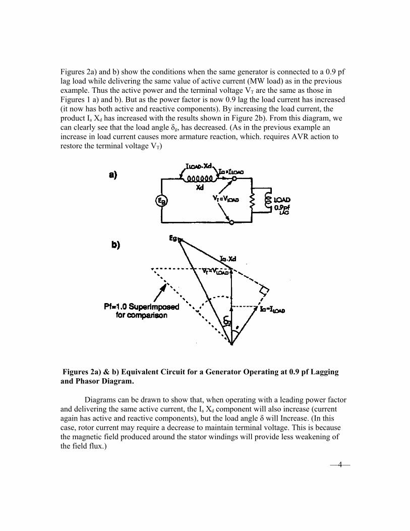
Figures 2a) and b) show the conditions when the same generator is connected to a 0.9 pf lag load while delivering the same value of active current (MW load) as in the previous example. Thus the active power and the terminal voltage VT are the same as those in Figures 1 a) and b). But as the power factor is now 0.9 lag the load current has increased (it now has both active and reactive components). By increasing the load current, the product Ia Xd has increased with the results shown in Figure 2b). From this diagram, we can clearly see that the load angle δg, has decreased. (As in the previous example an increase in load current causes more armature reaction, which. requires AVR action to restore the terminal voltage VT)

Figures 2a) & b) Equivalent Circuit for a Generator Operating at 0.9 pf Lagging and Phasor Diagram.

Diagrams can be drawn to show that, when operating with a leading power factor and delivering the same active current, the Ia Xd component will also increase (current again has active and reactive components), but the load angle δ will Increase. (In this case, rotor current may require a decrease to maintain terminal voltage. This is because the magnetic field produced around the stator windings will provide less weakening of the field flux.)

—4—

Variation of Transmission Line Load Angle With Load When a transmission line is loaded, a load angle δL is produced across the line.

Figure 3 a) shows the equivalent circuit for a line having a reactance of XL ohms and load is operating with a pf of cos θ lag. The resistance of the line is very small compared with its reactance, and will be neglected in this lesson. When the line is operating at 0.9 pf lag the supply voltage has to be considerably larger than the load voltage (which is kept constant). This is shown in the phasor diagram Figure 3 b). Note that a large load current Ia on the line having a large value of XL will give a large load angle δL

(a) (b)

Figures 3a) & b): Equivalent Circuit for a Transmission Line Operating at 0.9 Lag with Phasor Diagram

From the diagram, we can also see the result of changes in load angle caused by changes in load power factor (changes in θ). As θ becomes more lagging (increases clockwise) δL decreases. And conversely, as θ becomes more leading δL increases. Remember that this is only true in this example if the MW load remains constant.

—5—

Variation of Generator and Line Load Angle with Load

Figure 4 a) shows an equivalent circuit of a generator feeding a load via a transmission line. The generator operates with a load angle of δg and the line operates with a load angle of δL. The load is operating with a pf of cos θ.

b)

Figures 4a) & b): Equivalent Circuit for a Generator, Line and Load with Phasor Diagram

Note that: a) the generator operates at a power factor angle of θgen which is greater than θload

b) the generator and line operate together at an angle of δT, which is the sum of δg, and δL Any change in the load angle of the line or the generator, will result in a change in the total load angle for the generator/line.

—6—

SUMMARY OF THE KEY CONCEPTS • The load angle in a generator increases with increasing load current Ia • The load angle in a generator increases with operation at a more leading pf (decreasing excitation) if the MW load is held constant. • Conversely the load angle decreases with a decrease in load and/or operation at a more lagging pf (increasing excitation) if the MW load remains constant. • The load angle for a transmission line increases as the load on the line increases. As the load power factor for a transmission line becomes more leading the load angle will increase. • The total load angle for a generator/line is the sum of the individual load angles.

The Relationship Between Load Angle and Active Power Transfer.

In the system shown in Figure 4 a), the resistance of the generator and the lines is neglected, and consequently the system can be taken to be Loss free. ie there will be no active power loss between the generator terminals and the load.

As losses are neglected Pgen = Pload

If the line has reactance XL the true power flowing through the reactance to the load will be P = VT Vload sin δL /XL (1)

And, for the generator: P = EgVT sinδg /Xd (2)

The power transfer equation for the generator and line is:

P = Vload Eg sin( δg + δL ) / (Xd + XL) (3)

Equation 3 shows that for maximum active power transfer P:a) Xd and XL should be kept as small as possible. A generator has a value of Xd which cannot be altered. However, XL can be kept low by having short transmission lines or using many lines in parallel. b) Eg and VT and Vload should be kept at rated values. If they decrease load angle increases.

c) The composite load angle should not exceed 90°.

—7—

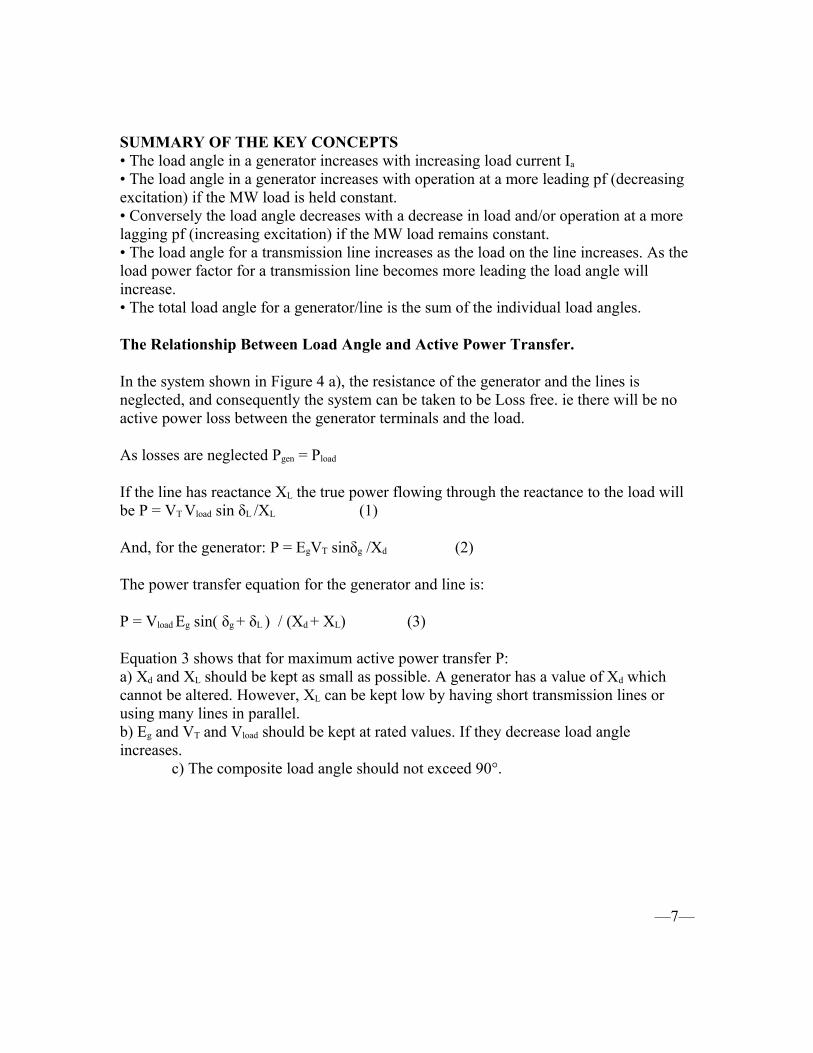
Transmission Line Steady State Stability Characteristics In the case of a loss free power line, the power at both ends of the line will be the

same.Pin = Pout = VTVload sinδ/XL

Pmax = VTVload /XL which occurs at δ = 90° and sinδ = 1

Pin = Pout = Pmax sinδTherefore the power transmitted or transferred from one end of the line to the other is a function of sinδ and a power transfer curve can be drawn, which has a sine wave shape.

Figure 5 shows curves & power P transmitted between two ends of a line having reactance XL, and voltages VT at one end and VL at the other. Generator characteristics are not included in this curve. When 100% power is being transmitted and the line is operating on curve 1 the line will have a load angle of δ1. If the sending end voltage VT is increased, then the power transfer capability for the line will be increased. When this happens, we shift to curve number 2 and the line will operate at an angle δ2 which is less than δ1. If the line voltage is decreased, the power transfer capability of the line will shift to curve 3 and angle δ3 and if the voltage is reduced further the line will operate on curve 4 and angle δ4.

Figure 5: STEADY STATE STABILITY PTC FOR TRANSMISSION LINES

—8—

When δ4 is reached, the line is operating at a 90° load angle. Any further reduction of the height of the curve or any further increase in power to be transferred will result in the power input exceeding the power that can be transferred. Assuming the mechanical power output from the turbine is constant, and line voltage decreases further, the generator will not be able to convert the mechanical power into electrical power. There will now be an excess of mechanical power produced over the electrical power being transferred. This excess power will cause the turbine generator shaft to accelerate. The net result is that the two ends of the line will no longer remain in synchronism and instability will result.

Applying these curves to a generator, as soon as the load angle exceeds 90° the power input to the generator will be greater than the power it can convert or transfer into electrical active power. Therefore the generator rotor will start to accelerate and, unless corrective actions are immediately taken, the generator will pole slip. The pole slip is the result of excessive mechanical input power causing the magnetic link between the generator and the electrical system to stretch excessively causing synchronism to be broken. The stronger the magnetic link between the generator and the electrical system, the more difficult pole slipping will be.

Try to visualize the magnetic link between the generator rotor and the electrical system as an elastic band. As the torque on the generator rotor increases, the elastic band connecting the rotor and the electrical system stretches, and the “load angle” between the rotor and the stator rotating magnetic field (RMF) increases. When the torque exceeds the strength of the elastic band (exceeds magnetic field strength), the band breaks, and the load angle continues to increase (pole slip). The stronger the elastic band, the harder it will be to break it (pole slip).

Steady state stability deals with slow changes in system conditions. This means that the movement between operating curves is a “slow” process, and load angle changes are small and slow. Thus, the “worst case” steady state condition will occur when the operating point moves to the peak of an operating curve, with δ = 90° (eg curve 4 shown in Figure5). Instability, as described above, will result if conditions change. The corrective actions that can be taken to avoid steady instability in this situation are: a) Reduction in turbine power Input. b) An increase in field current which will increase the flux and Eg (ie. cause the operating point to move to a “higher” curve)

Instability can be prevented by operating with total load angles well below stability limits. Maintaining a reasonable “operating margin” of load angle will ensure unstable conditions are not reached, even if transmission lines are removed from service. This will be shown in the examples below.

—9—

Examples

Practically, we can apply the above information to examples of transmission line/generator systems.

Example 1: A generator is operating at a load angle of 30° and transmitting power over two parallel lines. The load angle across the lines is 10°. If all the load is slowly shifted to one power line, will the line and generator remain stable? Answer: Using the power transfer equation for the line P = VTVL sinδL/XL

Transposing gives: sinδL = PXL / VTVL

If P, VT and VL remain constant then sinδL is proportional to XL.

When δL is 10° sin δL = 0.173 with reactance XL. When XL increases to 2 XL sin δL will increase to 2(0.173) = 0.347.This gives a new value δL2 for the line load angle where δL2 = arc sin 0.347 = 20.3°, ie the line load angle is approximately doubled. The combined load angle for the generator and line is 30° + 20.3° = 50.3° which is considerably less than 90° and so the generator and line will remain stable.

Example 2: A generator is operating at a load angle of 30° and transmitting power over 2 parallel lines. The load angle across the lines is 25°. If the load is slowly transferred to one line will the system remain stable?

Answer: Using the same power transfer equations as before and assuming P, VL and VT remain constant then sin δL is proportional to XL.This gives a new value of δL2 for the line load angle where δL2 = arc sin 0.845 =57.6°, this gives a combined load angle for the generator and line of (30° + 57.6°) = 87.6°. Under this condition the generator and line are operating at just less than 90° and will therefore remain sable. Any slight change in generator output or other conditions will cause the system to become unstable. It would be most undesirable to operate under these conditions.

Steady state stability deals with slow changes in the system. Rapid changes in the system will cause large swings in load angles. This is discussed in the following portion of the module.

—10 —

SUMMARY OF THE KEY CONCEPTS

• Active power transfer across power lines varies with the sine function of the total load angle δ. • Steady state stability is affected by total load angle, which is the sum of the generator load angle and line load angle. • If the load angle exceeds 90° stability will be lost, resulting in pole slipping.• To prevent steady state instability the mechanical power (input) must not exceed the power transfer capability of the generator and transmission line. Increased field flux increases internal voltage E and terminal voltage and causes a shift to a higher power transfer curve. • Operating without excessive load angles will ensure that stability limits are not reached, even under upset conditions.

—11 —

TRANSIENT STABILITY

Transient stability examines the behaviour of the generator and lines when faults or rapid changes occur. Remember that steady state stability involved gradual changes only. Transient stability can result in large swings of load angles, and possible instability (pole slipping).

GENERATORS Figure 6 shows two power transfer curves. Curve 1 is the power transfer curve

used when the generator supplies the load with normal excitation. When the excitation is reduced the power transfer capability is reduced to curve 2. The shape and height (amplitude) of the curves were discussed in a previous section of this module. There air two ways of modeling the generator response to a transient, the two curve, and the one curve method.

Figure 6: POWER TRANSFER CURVES FOR A GENERATOR

— 12 —

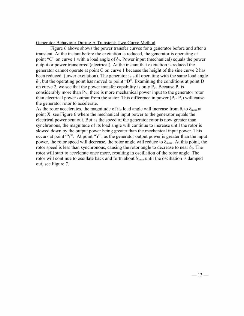
Generator Behaviour During A Transient: Two Curve Method Figure 6 above shows the power transfer curves for a generator before and after a

transient. At the instant before the excitation is reduced, the generator is operating at point “C” on curve 1 with a load angle of δ1. Power input (mechanical) equals the power output or power transferred (electrical). At the instant that excitation is reduced the generator cannot operate at point C on curve 1 because the height of the sine curve 2 has been reduced. (lower excitation). The generator is still operating with the same load angle δ1, but the operating point has moved to point “D”. Examining the conditions at point D on curve 2, we see that the power transfer capability is only P0 . Because P1 is considerably more than P0., there is more mechanical power input to the generator rotor than electrical power output from the stator. This difference in power (P1- P0) will cause the generator rotor to accelerate. As the rotor accelerates, the magnitude of its load angle will increase from δ1 to δmean at point X. see Figure 6 where the mechanical input power to the generator equals the electrical power sent out. But as the speed of the generator rotor is now greater than synchronous, the magnitude of its load angle will continue to increase until the rotor is slowed down by the output power being greater than the mechanical input power. This occurs at point “Y”. At point “Y”, as the generator output power is greater than the input power, the rotor speed will decrease, the rotor angle will reduce to δmean. At this point, the rotor speed is less than synchronous, causing the rotor angle to decrease to near δ1. The rotor will start to accelerate once more, resulting in oscillation of the rotor angle. The rotor will continue to oscillate back and forth about δmean until the oscillation is damped out, see Figure 7.

— 13 —

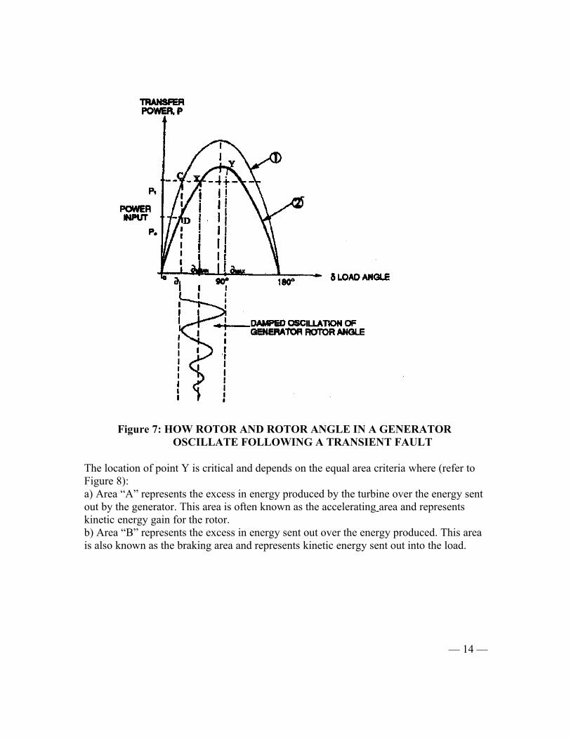
Figure 7: HOW ROTOR AND ROTOR ANGLE IN A GENERATOR OSCILLATE FOLLOWING A TRANSIENT FAULT

The location of point Y is critical and depends on the equal area criteria where (refer to Figure 8): a) Area “A” represents the excess in energy produced by the turbine over the energy sent out by the generator. This area is often known as the accelerating area and represents kinetic energy gain for the rotor. b) Area “B” represents the excess in energy sent out over the energy produced. This area is also known as the braking area and represents kinetic energy sent out into the load.

— 14 —

When area “A” = area “B”, the equal area criteria is satisfied, ie, the energy gained during acceleration is balanced by the energy sent out during braking.

Figure 8: EQUAL AREA CRITERIA WHERE AREA “A EQUALS AREA “B”

— 15 —

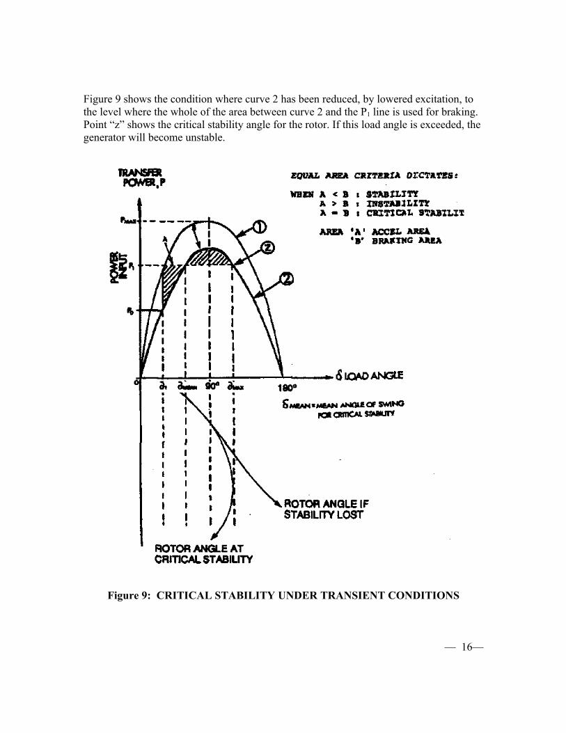
Figure 9 shows the condition where curve 2 has been reduced, by lowered excitation, to the level where the whole of the area between curve 2 and the P1 line is used for braking. Point “z” shows the critical stability angle for the rotor. If this load angle is exceeded, the generator will become unstable.

Figure 9: CRITICAL STABILITY UNDER TRANSIENT CONDITIONS

— 16—

Figure10(a) shows the condition where a generator remaims stable and Figure 10(b) shows the condition where a generator will become unstable. There is insufficient braking energy in this second case.

(a) (b)

Figure 10: TRANSIENT CONDITIONS SHOWING GENERATOR STABILITY AND INSTABILITY

Generator Behaviour During a Transient: One Curve Method. If only the normal operating curve and the maximum angle of swing are

known, then an examination of the curve and the conditions occurring at the maximum swing angle can determine whether the generator will remain stable. Figure11 shows the condition where a system transient caused the generator load angle to swing from δ1, to a maximum angle “A”. A transient increase in input power and/or a transient decrease in power transfer capability must have occurred. This could have been due to a transmission line fault or some other cause. At point “A”, the generator rotor angle has reached its maximum angle of swing and it is once more operating on the curve shown. At point “A”, there is an excess of power being transferred over the power being produced by the turbine. Consequently the rotor angle will decrease. A minimum angle will be reached before the angle increases again producing an angular oscillation which will decay after a short time. The generator will remain stable, see Figure 11.

— 17—

Figure11: GENERATOR REMAINS STABLE

If the swing angle shown at “B” is now considered, see Figure 12, The transient has caused the rotor load angle to exceed the critical angle δc and there is an excess of turbine power over the power being transferred. Consequently there is a resultant accelerating force and the load angle δ wIll continue to grow. The generator will pole slip and become unstable.

— 18—

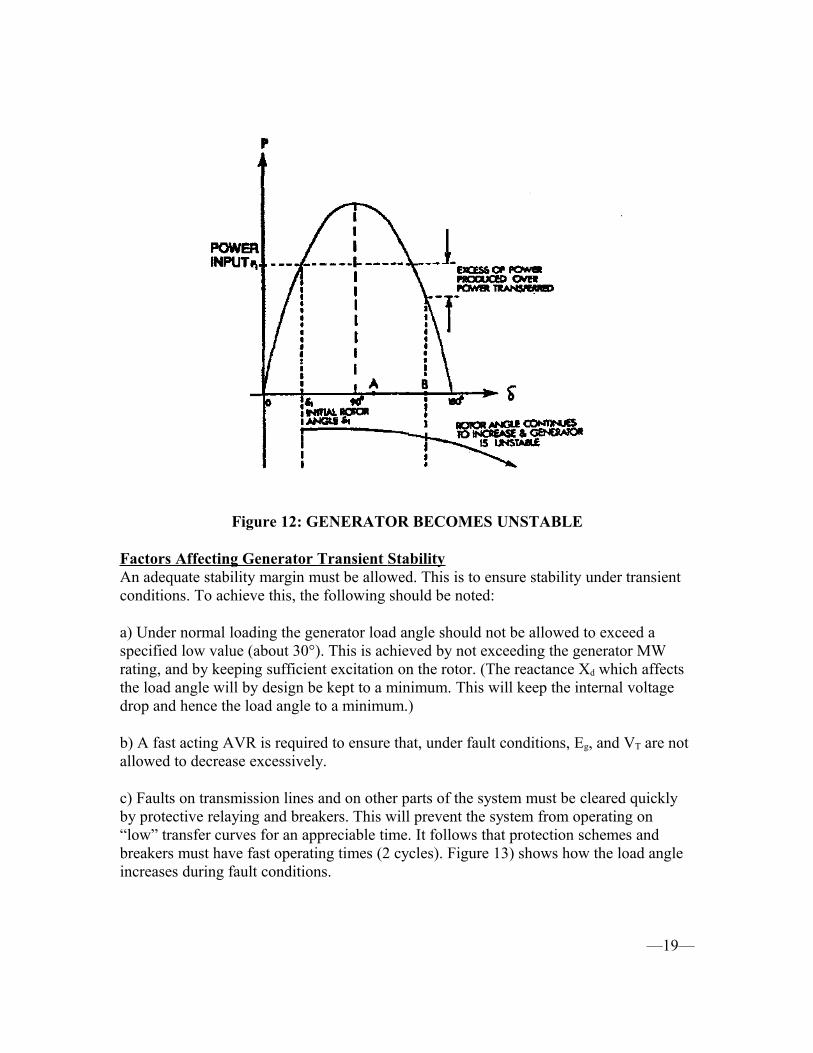
Figure 12: GENERATOR BECOMES UNSTABLE

Factors Affecting Generator Transient Stability An adequate stability margin must be allowed. This is to ensure stability under transient conditions. To achieve this, the following should be noted:

a) Under normal loading the generator load angle should not be allowed to exceed a specified low value (about 30°). This is achieved by not exceeding the generator MW rating, and by keeping sufficient excitation on the rotor. (The reactance Xd which affects the load angle will by design be kept to a minimum. This will keep the internal voltage drop and hence the load angle to a minimum.)

b) A fast acting AVR is required to ensure that, under fault conditions, Eg, and VT are not allowed to decrease excessively.

c) Faults on transmission lines and on other parts of the system must be cleared quickly by protective relaying and breakers. This will prevent the system from operating on “low” transfer curves for an appreciable time. It follows that protection schemes and breakers must have fast operating times (2 cycles). Figure 13) shows how the load angle increases during fault conditions.

—19—

d) Another factor to be considered is that generators should have large inertias, which will slow the rate of increase in load angle under transient conditions. This is a design constant over which we have no control. We will ignore this factor’s contribution from a stability viewpoint.

Figure13: HOW LOAD ANGLE INCREASES DURING A FAULT

The upper curve in Figure 13) represents power transfer under healthy conditions. For this example, let’s assume that this represents power transfer through three parallel lines transmission lines, If a line is temporarily lost due to a lightning strike, power transfer is shifted to the capacity of the two remaining lines. This shifts the operating point to “B” on the lower curve. Since the power produced is still at P0, which is greater than the power that can be transferred the turbine generator rotor will accelerate, and the load angle increases. When the fault clears and the line is restored, the power transfer will return to the upper curve. The maximum swing of the load angle after the fault clears will again be determined by the equal area criteria (area A-B-C-D = area D-E-F-G). It follows that the longer the fault persists the longer the generator is operating on the lower curve and the greater the load angle becomes with a greater risk of instability.

-20-

Transient Stability: Transmission Lines The power transfer capability of a transmission line is proportional to the product

of the supply and load end voltages. To keep the power transfer capability to its maximum, and for the line to remain stable under transient conditions, the following features are employed: a) Fast acting AVRs are used on the generators at the supply end. This keeps the supply voltage constant. b) Synchronous condensers and capacitors are used to keep the load end voltages almost constant. Having an interconnected system will also aid in keeping the load voltage constantc) The reactance XL in ohms per kilometer for a line is essentially constant and the only way of reducing XL is to operate with short transmission lines, and using more lines in parallel. Although we cannot change the distance to the loads, we can control the number of lines. d) As with generators, fast acting protection schemes and breakers are required to minimize the time that transient conditions exist.

Examples A generator and transmission system are operating at point P1 on curve 1 shown

in Figure14. Between the generator and the load are two transmission lines. Due to a lightning strike, one line trips and the generator and. remaining line operate on curve 2. Explain whether the generator and line will remain stable. If the generator remains stable, show the maximum and mean angles of swing and sketch in any oscillations in load angle.

Figure14: PTC FOR A GENERATOR AND TRANSMISSION LINES

-21-

Answer:

The equal area criteria must be satisfied for stability. Figure15 shows the power transfer curves for a generator and two lines (Curve 1), and a generator and one line (Curve 2). Area “A” represents the condition where the power input from the turbine is greater than the power being transferred and the generator rotor accelerates. The rotor speed and hence load angle δ increases. Area “B” represents the condition where the output power is greater than the turbine power and the generator rotor brakes or slows down, this causes δ to decrease. The equal area criteria are satisfied and stability is maintained.

Figure 15: TRANSIENT STABILITY

When the line trips, the rotor and line load angle will increase to δmax, because the input power is greater than the power being transferred. But, at the δmax point, because the power output is greater than the power input, the load angle will begin to reduce (eventually to a value near δ1). The load angle will oscillate and finally stabilize at a steady value of δmean (see diagram). The braking energy available was greater than the accelerating energy so the critical angle was not attained and the generator and line remain stable.

-22-

Question:

The power transfer curve for a generator is shown in Figure16. Due to a transient system disturbance the load angle δ increases. A, B and C on the diagram, are maximum angles of swing for the three different system disturbances. For each disturbance explain whether the generator would remain stable or unstable. If the generator remains stable, show on your diagram the angle at which the generator will stabilize; if it is unstable show how the angle continues to increase.

Figure16: POWER TRANSFER CURVE FOR A GENERATOR

Answer: Only one power transfer curve is given together with the maximum load angle for

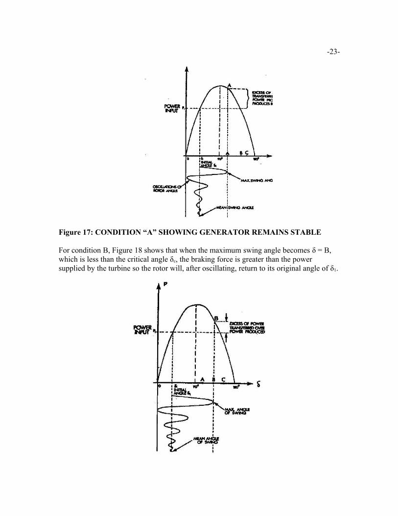
each condition. Therefore assume that the generator only operates on this curve. The Input power to the generator, P1 is constant. When the power being supplied by the generator is greater than P1, the generator rotor brakes or decelerates. When the power being supplied by the generator is less than P1 the generator rotor accelerates. It is this acceleration /deceleration that produce the change in load angle δ. Figure 17 shows that when P1 is less than the power being transferred (point “A’, which is less than the critical angle δc, on the PTC), the excess power transferred over that supplied by the turbine creates a braking force and the generator rotor will decelerate. Therefore δ decreases and after oscillating, will return to its original angle of δ1. The generator will remain stable.

-23-

Figure 17: CONDITION “A” SHOWING GENERATOR REMAINS STABLE

For condition B, Figure 18 shows that when the maximum swing angle becomes δ = B, which is less than the critical angle δc, the braking force is greater than the power supplied by the turbine so the rotor will, after oscillating, return to its original angle of δ1.

Figure 18: CONDITON “B” SHOWING GENERATOR REMAINS STABLE

-24-

For condition C, Figure19 shows that when the maximum swing angle becomes δ = C, which is greater than the critical angle δc the braking force is less than the turbine force (P1 is greater than the power being transferred) so the rotor will not return to its original angle of δ1. The rotor angle will continue to increase and the generator rotor will pole slip.

Figure 19: CONDITION “C” SHOWING GENERATOR BECOMES UNSTABLE

-25-

SUMMARY OF THE KEY CONCEPTS

* Transient instability can result in pole slipping.

For the generator:

* Control of generator load angle will help ensure transient stability. Exceeding generator MW rating should be avoided. * AVRs are used to keep generator terminal volts VT constant and improve stability. * Protection schemes and breakers must rapidly clear faults to prevent large swings in load angles during transient conditions. * Preventive maintenance and testing are important to ensure that protection schemes are operational.

For the transmission line:

* Multiple power lines are used in parallel ( keep XL low). * Automatic voltage regulation is used to keep supply end voltage

constant. * Synchronous condensers and interconnections are used to keep load end volts constant. This minimizes voltage drops reducing chances of transient instability.* Protection schemes and breakers must rapidly clear faults.

-26-