GASMODGas Pipeline Hydraulic Simulation

Version 7.0

www.systek.us

LICENSE AGREEMENT AND LIMITED WARRANTY

You should carefully read the following terms and conditions. Your using of this Program indicates your acceptance of them. If you do not agree with this terms and conditions, you should promptly return the complete package and your money will be refunded.

SYSTEK provides this Program and licenses its use to you. You are responsible for selecting the Program to achieve your intended results and for the installation, use and results obtained from the program.

This Program is a proprietary product of SYSTEK and is protected by copyright laws. Title to the program, or any copy, modification or merged portion of the Program shall at all times remain with SYSTEK. It is licensed for use for a specified period as described below.

LICENSE

This software package is licensed to an individual or a company for a period of five years from the date of payment of the license fee. If the software is leased, the license is valid for the period of the lease only. Continued use of the software requires renewal or extension of the license by payment of a renewal fee, determined by SYSTEK at the time of renewal. As a licensed user, you may:a. Use the Program on a single machine. The Program may be transferred to and used on another machine but shall under no circumstances be used on more than one machine at a time. If SYSTEK designates the Program as a network Program, it may be used on a network system approved by SYSTEK.

b. Transfer the Program together with this License to another person, but if only the other person agrees to accept the terms and conditions of this Agreement. If you transfer the Program and the License, you must at the same time either transfer all copies of the Program and its Documentation to the same person or destroy those not transferred. Any such transfer terminates your License.

You may not:a. Transfer or rent the Program or use, copy, modify or merge the Program in whole or in part except as expressly permitted in this License.

b. Decompile, reverse assemble or otherwise reverse engineer the Program.

c. Reproduce, distribute or reverse the program documentation.

IF YOU DO ANY OF THE FOREGOING, YOUR RIGHTS UNDER THIS LICENSE WILL AUTOMATICALLY TERMINATE. SUCH TERMINATION SHALL BE IN ADDITION TO AND NOT IN LIEU OF ANY CRIMINAL, CIVIL OR OTHER REMEDIES AVAILABLE TO SYSTEK.

LIMITED WARRANTY EXCEPT AS SPECIFICALLY STATED IN THIS AGREEMENT, THE PROGRAM IS PROVIDED AND LICENSED "AS IS" WITHOUT WARRANTY OF ANY KIND, EITHER EXPRESSED OR IMPLIED INCLUDING BUT NOT LIMITED TO, THE IMPLIED WARRANTIES OF MERCHANTABILITY AND FITNESS FOR A PARTICULAR PURPOSE.

SYSTEK warrants the Program will substantially perform the functions or generally conform to the Program's specifications published by SYSTEK and included in this package.

SYSTEK does not warrant that the functions contained in the Program will meet your requirements or that the operation of the Program will be entirely error free or appear precisely as described in the Program documentation.

LIMITATION OF REMEDIES AND LIABILITY

The remedies described below are accepted by you as your only remedies and shall be available to you only if you or your dealer returns the enclosed registration form to SYSTEK within ten days after delivery of the Program to you.

SYSTEK's entire liability and your exclusive remedies shall be:a. If the Program does not substantially perform the functions or generally conform to the Program's specifications published by SYSTEK, you may within 30 days after delivery, write to SYSTEK to report a significant defect. If SYSTEK is unable to correct that defect within 30 days after receiving your report, you may terminate your License and this Agreement by returning the Program disk and Hardware key security device and your money will be refunded. All copies of the Program in your possession shall be deleted or destroyed.

If this software was acquired as part of a training class or workshop, the above refund privileges do not apply. No refund will be provided.

b. If the Program disk is defective within 30 days of delivery, you may return it and SYSTEK will replace it.

TO THE MAXIMUM EXTENT PERMITTED BY APPLICABLE LAW, IN NO EVENT WILL SYSTEK BE LIABLE TO YOU FOR ANY DAMAGES INCLUDING LOST PROFITS, LOST SAVINGS, OR OTHER INCIDENTAL OR CONSEQUENTIAL DAMAGES , ARISING OUT OF THE USE OR INABILITY TO USE THE PROGRAM, EVEN IF SYSTEK OR DEALER AUTHORIZED BY SYSTEK HAS BEEN ADVISED OF THE POSSIBILITY OF SUCH DAMAGES.

GENERALThis Agreement will be governed by and construed in accordance with the laws of the State of Delaware.

Any questions concerning this Agreement should be referred in writing to SYSTEK at the address shown at the web site or email at the address shown in the Technical Support section of the manual:

Email: support@systek.us

Web site: www.systek.us

YOU ACKNOWLEDGE THAT YOU HAVE READ THIS AGREEMENT AND BY USING THIS PROGRAM INDICATE YOUR ACCEPTANCE OF ITS TERMS AND CONDITIONS. YOU ALSO AGREE THAT IT IS THE COMPLETE AGREEMENT BETWEEN US AND THAT IT SUPERSEDES ANY INFORMATION YOU RECEIVED RELATING TO THE SUBJECT MATTER OF THIS AGREEMENT.

Copyright 1982-2015 SYSTEK. All rights reserved. No part of this program may be reproduced, stored in a retrieval system, or transmitted, in any form or by any means, electronic, mechanical, photocopying or otherwise, without the prior permission of SYSTEK.

Version 7.00August 2015

Table of Contents1. Introduction.............................................................................................................................................5

3 GASMOD

2. Getting Started........................................................................................................................................7

2.1 Installation – Internet Authenticated Version...................................................................................7

2.2 Retaining/Releasing - Internet Authenticated Version......................................................................8

2.3 Installation on a Network..................................................................................................................8

2.4 Un-installation...................................................................................................................................8

3. Features...................................................................................................................................................9

3.1 Running the Program.......................................................................................................................11

4. Tutorial..................................................................................................................................................18

4.1 Sample Problem...............................................................................................................................18

4.2 Solution............................................................................................................................................21

4.3 File Format for Pipe Data File..........................................................................................................32

4.4 Pipe Branches..................................................................................................................................35

4.5 Pipe Loops.......................................................................................................................................39

4.6 Building pipeline model graphically.................................................................................................41

4.7 Locating Compressor Stations.........................................................................................................48

4.8 Quick Start Option...........................................................................................................................50

4.9 Quick Pressure Drop........................................................................................................................52

4.10 Cost calculations............................................................................................................................54

5. Reference.............................................................................................................................................57

5.1 Hydraulic Formulas..........................................................................................................................57

5.2 Cost Formulas..................................................................................................................................62

6. Troubleshooting....................................................................................................................................64

6.1 Error Messages:...............................................................................................................................64

7. Technical Support..................................................................................................................................65

7.1 How to contact us............................................................................................................................65

8. Sample Reports.....................................................................................................................................66

Sample Problem –1 (English Units)........................................................................................................67

Sample Problem –2 (English Units)........................................................................................................74

1. Introduction

4 GASMOD

GASMOD is a steady state, single phase, hydraulic simulation software for gas pipelines considering heat transfer between the pipe and the surrounding medium. Multiple compressor stations along the pipeline may be modeled. Calculations are performed for a given flow rate and gas properties. Gas may be injected or delivered at various locations along the pipeline. The inlet gas stream compositions, if available, may be input instead of the gas properties. Branch pipes off the main pipeline may be modeled. Pipe segments can be looped. The pipeline may be bare or insulated. The thermal conductivity of the pipe, insulation and surrounding soil may all be varied along the entire length of the pipeline, or an overall heat transfer coefficient may be specified. Calculated results include pipeline pressure and temperature profile, compressor station HP required and fuel consumption.

The pipe absolute roughness, used in friction drop calculations may also be varied along the pipeline, facilitating the analysis of internally coated and uncoated pipelines. Pressure drop is calculated using one of the various equations (such as General Flow Equation, AGA, Colebrook-White, Panhandle, etc.). The compressibility factor may be calculated using one of the three options: Standing-Katz, AGA and CNGA methods. Pipeline elevations are taken into account in determining the pressures and horsepower required at each compressor station.

The pipeline pressures, temperatures, compressor station suction and discharge pressures and compressor horsepower required are calculated and output on the screen. Gas fuel consumption for turbine driven compressor stations can also be calculated. For new pipelines and for preliminary studies, the locations of compressor stations can be determined. Results of each calculation are also saved to a disk file.

Multiple cases may be easily modeled quickly and accurately. GASMOD is ideal for the design of a new gas pipeline or checking capabilities of existing gas pipelines. The hydraulic gradient showing the pipeline pressures can also be plotted.

For preliminary feasibility studies, GASMOD includes an option for calculating the capital cost and the annual operating cost of the pipeline. Using this, the annual cost of service and transportation tariff may be calculated.

Most data are entered in Microsoft Excel compatible spreadsheets that results in easy editing and cut and paste operations via the Windows clipboard. All pipeline data including the pipeline profile (distance, elevation, pipe diameter, wall thickness, pipe roughness and MAOP) are saved in .TOT file.  All gas properties are stored in a common Gas Properties Database files. Help is available on each data entry screen and on the status bar at the bottom of each data entry screen.

5 GASMOD

Beginning with GASMOD Version 6, the pipeline model may be created graphically. In this method, objects such as pipe segments, valves, compressor stations and other devices may be selected from a toolbox and dropped on a drawing canvas. These objects can be connected with pipe segments to form the pipeline system. The properties of each object may be defined by double-clicking on them and entering data in the screen that is displayed. A video tutorial is available that explains how the pipeline model can be created graphically. Check the following link https://www.youtube.com/watch?v=zMDCHT1iY5M

A toolbar consisting of icons for commonly used menu items such as File Open, Save, Print, Run etc. is available below the menu bar. These menu items or commands can be accessed by clicking on the icons. As the mouse is moved over an icon, a tool tip HELP appears explaining the function of each icon on the toolbar.

The results of the simulation are displayed on the screen in a scrollable window, as well as saved on a disk for later viewing or printing. A printed hard copy of the calculated results can be generated, after reviewing the screen output. Customized output reports may be generated, consisting of short or long reports.

This software can be run on Pentium and Athlon based computers and compatibles with a minimum of 8 GB RAM running Microsoft Windows XP/7/8/10 operating systems. A minimum hard disk space of 25 MB is required for installing the program.

6 GASMOD

2. Getting StartedThe software program is supplied on a CD-ROM that must be installed on your computer’s hard disk as described below.

This single user license entitles you to use the software only on one computer at a time. If you purchased a multi-user or network license, you are entitled to use the software on more than one computer as described in other documentation that accompanied the software.

2.1 Installation – Internet Authenticated VersionBefore starting the installation process, close all currently running programs and turn off any virus checking software, if present on the hard disk. If you want to ensure that the program disk is free of any virus you may run the virus scanning software and check the program CD prior to starting installation.

1. Insert the software CD into the CD-ROM drive.

2. Run as administrator “Setup.exe”

Follow the subsequent screen instructions to continue with the installation process.

After the setup is completed, the User Registration screen will prompt you to enter your name, company name and the program serial number. The serial number found on the program CD container must be entered exactly. Otherwise the installation will be incomplete.

Note that Windows 7/8/10 require installing software with administrative privileges. Therefore, disable the automatic setup and run the “setup.exe” program from the CD-ROM as an Administrator.

Follow the subsequent screen instructions to continue with the installation process.

After the setup is completed, the User Registration screen will prompt you to enter your name, company name and the program serial number. The serial number found on the program CD container must be entered exactly. Otherwise the installation will be incomplete.

You must be connected to the Internet to register the program and obtain a license. Otherwise you will not be able to run the software after installation.

Once installation is completed, a program icon and program folder will be automatically created. You may pin a shortcut to the Taskbar.

7 GASMOD

2.2 Retaining/Releasing - Internet Authenticated VersionTo launch the program, you will click the program icon from the Program menu. If the program is properly registered and the license obtained, you will be able to start the program.

In order to use the program on another computer, you may release control of the license of this program. This is done by Clicking HELP followed by Release Control. This enables you to quit the program on your work computer, release control and restart the program on your home computer or on a laptop while traveling. However each time you quit the program you must release control if you want to run the program on another computer. Also, internet access is required to do this.

Remember that once a program is registered and control is retained on the computer, the license can only be released from that computer.

2.3 Installation on a Network If you are licensed to use the program in a network environment, the software may be installed on multiple workstations on your network. The software can then be run from any workstation on the network, subject to the maximum user limit programmed during the installation process and in accordance with your license. PLEASE REVIEW SEPARATE DOCUMENTATION ON LAN/WAN INSTALLATION SUPPLIED WITH PROGRAM.

2.4 Un-installationTo uninstall the software from the hard disk, go to the Windows Start button and choose Settings. Next select the Control Panel and click on Add/Remove (Uninstall) Programs. Follow subsequent instruction to uninstall GASMOD. All pipeline models and gas properties database are located in My Documents\GASMOD\ folder and maybe backed up for future use.

Put your original program disk away safely.

8 GASMOD

3. FeaturesGASMOD is a powerful steady state thermal hydraulic simulation program for gas pipelines with multiple compressor stations. Despite the complexity of the program it is very user-friendly. Online HELP is available for most data entry screens and the program has extensive error checking features.

The pipeline model may be created graphically using a drag and drop approach. In this method, objects such as pipe segments, valves, compressor stations and other devices may be selected from a toolbox and dropped on a drawing canvas. These objects can be connected with pipe segments to form the pipeline system. The properties of each object may be defined by double-clicking on them and entering data in the screen that is displayed. A video tutorial is available that explains how the pipeline model can be created graphically. This is also available under Help|General Help.

Simulates steady state, single phase hydraulics of a pipeline transporting a gas or compressible fluid, considering heat transfer between the gas and the surrounding medium (soil in a buried pipeline).

Gas may be injected or delivered at various points along the pipeline. Gas composition may be specified as well.

The pipe diameter, wall thickness, pipe roughness, thermal conductivity, insulation thickness and the surrounding soil temperatures and soil thermal conductivity can all be varied throughout the length of the pipeline.

The available pressure drop formulas include AGA Turbulent, Colebrook-White, General Flow Equation, IGT, Panhandle A & B, and Weymouth equations.

Gas compressibility factor calculation options include Standing-Katz, AGA and CNGA methods.

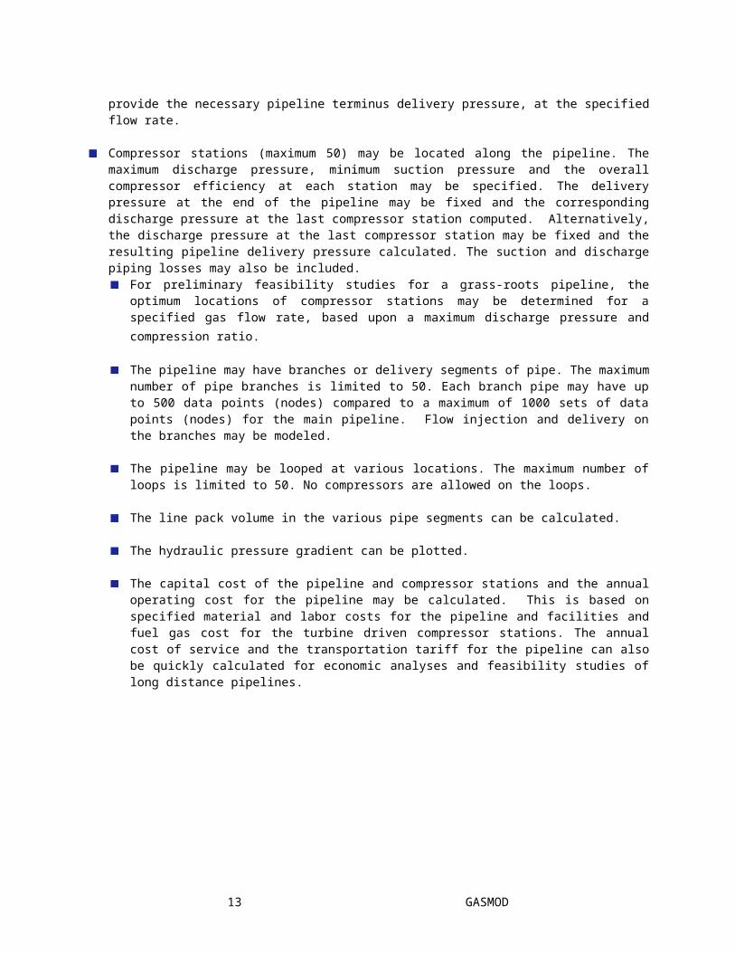
The pipeline may be modeled with a head compressor station at the origin of the pipeline or by specifying an inlet pressure, such as a connection to another pipeline. In some cases, the first compressor station may be located downstream at some distance from the pipeline origin. The pipeline inlet pressure must be sufficiently high to provide the necessary suction pressure to the first compressor station. In the case of a short pipeline with no compressor stations, the inlet pressure must be sufficient to provide the necessary pipeline terminus delivery pressure, at the specified flow rate.

Compressor stations (maximum 50) may be located along the pipeline. The maximum discharge pressure, minimum suction pressure and the overall compressor efficiency at each station may be specified. The delivery pressure at the end of the pipeline may be fixed and the corresponding discharge pressure at the last compressor station computed. Alternatively, the discharge pressure at the last compressor station may be fixed and the resulting pipeline delivery pressure calculated. The suction and discharge piping losses may also be included.

For preliminary feasibility studies for a grass-roots pipeline, the optimum locations of compressor stations may be determined for a specified gas flow rate, based upon a maximum discharge pressure and compression ratio.

9 GASMOD

The pipeline may have branches or delivery segments of pipe. The maximum number of pipe branches is limited to 50. Each branch pipe may have up to 500 data points (nodes) compared to a maximum of 1000 sets of data points (nodes) for the main pipeline. Flow injection and delivery on the branches may be modeled.

The pipeline may be looped at various locations. The maximum number of loops is limited to 50. No compressors are allowed on the loops.

The line pack volume in the various pipe segments can be calculated.

The hydraulic pressure gradient can be plotted.

The capital cost of the pipeline and compressor stations and the annual operating cost for the pipeline may be calculated. This is based on specified material and labor costs for the pipeline and facilities and fuel gas cost for the turbine driven compressor stations. The annual cost of service and the transportation tariff for the pipeline can also be quickly calculated for economic analyses and feasibility studies of long distance pipelines.

10 GASMOD

3.1 Running the ProgramTo run the program, click the GASMOD program icon from the desktop short cut The GASMOD program will be installed in the default folder C:\Program Files (x86)\SYSTEK\GASMOD. All pipeline model files that are created will be located in the My Documents\GASMOD folder.

The initial program screen will be displayed as follows:

11 GASMOD

An introductory screen shown below describes the five steps necessary to solve a typical pipeline problem using GASMOD.

12 GASMOD

Next the Startup options screen is displayed:

In the above screen four options are presented:

Open last pipeline model: To continue with the last pipeline model file. Create new pipeline model in spreadsheet: This allows you to build a pipeline model from scratch by inputting data in a spreadsheet

Create the pipeline model graphically: This allows you to build a pipeline model from scratch using the graphic tools.

Quick Start: This allows you to quickly build a pipeline model by specifying some basic data on the pipeline, gas flow rate and gas properties. This is described in more detail under the title Quick Start Option.

13 GASMOD

The menu bar along the top of the Main screen has several pull down options under each menu item, such as File, Edit etc. as explained below.

A toolbar consisting of icons for commonly used menu items is available below the menu bar. These menu items or commands can be accessed by clicking the icons. As the mouse is moved over an icon, a tool tip help appears explaining the function of each icon.

The pull down menu under File has the following options:

New - To create a new pipeline data file using the spreadsheet or graphic model option.

Open - To open and edit an existing pipeline data file.View - To view the results of the last simulation or the pipeline (TOT file).Save - To save the current data file on the hard drive under the current

file name.Save As - To save a pipeline data file under a new name.Close - To close a pipeline data file.Page setup - To set up the margins for the printed output and

selecting the printer.Print Preview – For viewing before printingPrint - To print the spreadsheet file or the last simulation report file.Send Email - To send an email of a spreadsheet file or an output

file to an associate or to SYSTEK for technical support.Exit - To quit the program

The pull down menu under Edit has the following:

Cut - To remove selected (highlighted) data from the spreadsheet to the Windows clipboard.

Copy - To copy selected (highlighted) data from the spreadsheet to the Windows clipboard.

Paste - To paste the data from Windows clipboard to the current cursor location in the spreadsheet.

Fill down - Select the rows to be filled down and click. This will fill down with the same numbers as above.

Insert row - To insert a new row in the spreadsheet Delete row - To delete a row in the spreadsheet.Format Cells - To format individual cells in the spreadsheet.

Accelerator keys, such as Ctrl-X for Cut and Ctrl-I for Insert row are available for several menu items.

14 GASMOD

The pull down menu under Options has the following:

Units - For selecting English (US Customary units) or SI-Metric units of calculation. Also to specify other units of measurement, such as pipeline distance, the gas flow rate, pressures and temperature.

Global Parameters - For specifying the ratio of specific heats of gas (Cp/Cv), the maximum gas velocity in the pipeline, the pipeline efficiency, the base temperature and base pressure. Also you can choose the desired pressure drop formula such as AGA, Colebrook-White, etc. and Compressibility factor method. Available options for the compressibility factor are: CNGA, Standing-Katz or AGA NX19 method. In addition, you can select Joule-Thompson cooling effect in the calculations, if desired. If Joule-Thompson cooling effect is considered, less conservative results (lower pressure drop for given flow rate due to cooler gas temperatures) will be obtained. Neglecting this cooling effect will cause slightly higher pressure drops for a given flow rate.

Interpolate Elevation - To interpolate the elevation of pipeline at an intermediate milepost.

Quick Start - To quickly build a pipeline model by specifying some basic pipe, gas flow rate and properties data. This is described in detail in a later section.

The pull down menu Station gives you the following choices

Compressor Stations - This lets you specify the compressor station locations along the pipeline. This is the same as clicking the Stations button on the left panel. In this option, you may specify the compressor station name, mile post location, compressor efficiencies and mechanical efficiencies. In addition, minimum suction and maximum discharge pressures, maximum discharge temperature, and the suction and discharge piping losses are input in this screen. Only the suction pressure at the first compressor station is used by the program. The suction pressures at all other compressor stations are calculated for the specified discharge pressures and flow rates. At the end of the pipeline, if a particular delivery pressure is required, the discharge pressure of the last compressor station will be adjusted to provide the desired pipeline terminus pressure. To turn on this option, a check box is provided in the main pipeline spreadsheet as below.

In addition to specifying the compressor station data, the fuel gas consumption for gas turbine driven compressors can also be calculated as an option by checking the box on the bottom left of this screen.

If there are no compressor stations, or if the first compressor station is not located at the origin (first milepost) of the pipeline, it is assumed that there is a connection to another pipeline that provides the pressure at the pipeline origin. In this case, a screen is displayed for specifying the pipeline inlet pressure.

15 GASMOD

16 GASMOD

Locate Compressor Stations – Determines the number and approximate locations of the compressor stations required for a specified gas flow rate, based upon a maximum discharge pressure and compression ratio.

Valve Stations - This is used for specifying minor and major pressure drop devices. These include valves, fittings, pressure regulators and other custom components such as meters and filters along the pipeline. The resistance coefficient or K-values needed for calculating the minor losses through valves and fittings are built into the program. You may also specify the actual pressure drop through a valve, fitting or custom device. In the latter case, the K-value is not used. To model a pressure regulator, you must indicate the downstream pressure required at a milepost location where the regulator will be installed. 

The menu item Gas Flow is for specifying the locations (milepost) where gas enters and exits the pipeline. This is the same as clicking the Flow rates button on the left panel. Additionally, the mile post location measured from the beginning of the pipeline, the gas flow rate, positive for incoming flow and negative for a delivery out of the pipeline, are also input. The flow rate at the first mile post must always be positive, indicating inflow. The gas temperature, specific gravity (Air = 1.0) and viscosity are also input here. Alternatively, instead of gas gravity and viscosity, you may input the compositional data for the gas stream. GASMOD will calculate the gas properties from the mole composition. This is described in detail later. Under Gas Flow is the Gas Properties Database which is used to enter the Gas properties or compositions for use with the program.

The menu item Conductivity is for entering the thermal conductivity data for heat transfer calculations. This is the same as clicking the Conductivity button on the left panel. The pipe burial depth, insulation thickness, thermal conductivity of pipe material, insulation and the surrounding soil and soil temperature can be input. A fixed, overall heat transfer co-efficient may also be specified instead of the thermal conductivities.

The menu item Branch is used for specifying incoming and outgoing pipe branches off the main pipeline. This option is also used for defining pipe loops. Refer to the sections titled Pipe Branches and Pipe Loops for more information.

The pull down menu under Run has the following:Go! - This starts simulation after saving all data entered

This is the same as clicking the Calculate button on the left panel.

The menu under Graphics is used for plotting the pipeline hydraulic pressure gradient and temperature gradient.

The menu HELP|About gives you information on the registered User, version number and serial number. In addition you can release control of your license, get general help, intro screen and demo parameters. Help is also available on each data entry screen and on the status bar at the bottom of each data entry screen. Answers to specific queries such as “How to create a pipe data file” can be found under How Do I? on the left panel.

17 GASMOD

The toolbar icon designated as Q is used for quickly calculating the pressure drop in a pipe segment for isothermal flow. Clicking this icon brings up a data entry screen for calculating the pressure drop in a pipe segment for a given flow rate, pipe diameter, pipe length, gas properties and pipe inlet or delivery pressure. For details refer to the section titled Quick Pressure Drop.

The toolbar icon designated as $ is used for calculating the capital and operating costs of the pipeline for performing quick economic analyses. The annual cost of service and the tariff required can also be calculated. This is discussed in detail under the Cost Calculations section.

In addition to the horizontal menu bar and the toolbar icons, the vertical panel on the left also provides options to activate most menu items as indicated below:

Create a new pipeline using the spreadsheet option or graphic model builder

Build a new pipeline model using the graphic model builder

Lets you define the compressor station locations along the pipeline.

Lets you specify valves, fittings, custom devices and pressure regulators

For specifying the locations, temperature and gas properties, where gas enters and exits the pipeline

Enter the thermal conductivity and soil temperature data.

To start simulation

To view simulation reports.

For Help on specific topics

Exit the program

18 GASMOD

4. Tutorial

This section leads you through the program, using an illustrative example. The results of the simulations are included in the Sample Reports section. Several additional sample problems, involving pipe branches and pipe loops and the simulation runs are included in the program. See the Reference section for an explanation of the symbols and formulas used in this program.

4.1 Sample ProblemAn 18-inch/16-inch diameter, 420 mile long buried pipeline defined below is used to transport 150 MMSCFD of natural gas from Compton to the delivery terminus at Harvey. There are three compressor stations located at Compton, Dimpton and Plimpton, with gas turbine driven centrifugal compressors. The pipeline is not insulated and the maximum pipeline temperature is limited to 140 deg F due to the material of the pipe external coating. The maximum allowable operating pressure (MAOP) is 1440 psig. Determine the temperature and pressure profile and the horsepower required at each compressor station.

19 GASMOD

The pipeline profile is defined below:

Distance Elevation Pipe dia. Wall thick. Roughness(miles) (ft) (in) (in) (in)

0.0 620 18.00 .375 0.00070045 620 18.00 .375 0.00070048 980 18.00 .375 0.00070085 1285 16.00 .375 0.000700160 1500 16.00 .375 0.000700200 2280 16.00 .375 0.000700238 950 16.00 .375 0.000700250 891 16.00 .375 0.000700295 670 16.00 .375 0.000700305 650 16.00 .375 0.000700310 500 16.00 .375 0.000700320 420 16.00 .375 0.000700330 380 16.00 .375 0.000700380 280 16.00 .375 0.000700420 500 16.00 .375 0.000700

Gas specific heat ratio : 1.26Maximum Gas velocity : 50 ft/secPipeline efficiency : 1.00Base temperature : 60 deg FBase pressure : 14.70 psia.Pressure drop formula : Colebrook-WhiteCompressibility factor : Standing-Katz

A flow rate of 150 MMSCFD enters the pipeline at Compton (milepost 0.0) and at an intermediate location named Doodle (milepost 85), a delivery of 20 MMSCFD is made. Additionally, an injection of 10 MMSCFD is made at Kreepers (milepost 238). The resulting flow then continues to the end of the pipeline. Gas inlet temperature is 70 deg F at both inlet locations.

Inlet Gas specific gravity (air = 1.00) : 0.600Inlet Gas Viscosity : 0.000008 lb/ft-sec

20 GASMOD

The compressor stations are as follows:

Compressor Location Discharge Press. station (miles) (psig) Compton 0.00 1400Dimpton 160.0 1400Plimpton 295.0 1400

The installed HP at each compressor stations is 5,000 HP

Origin suction pressure : 800 psig.Pipeline delivery pressure : 500 psig.Minimum pipe pressure : 200 psig.Station suction loss : 5 psigStation discharge loss : 10 psigCompressor adiabatic efficiency : 85 %Compressor mechanical efficiency : 98 %Fuel consumption : 0.2 MCF/day/HP

Pipe burial depth : 36 inchesPipe thermal conductivity : 29 Btu/hr/ft/deg FSoil thermal conductivity : 0.800 Btu/hr/ft/deg FAmbient soil temperature : 65 deg FOrigin suction temperature : 70 deg F

A printed copy of the output from the above sample problem is included in this manual under the section heading Sample Reports. In addition, printed output of calculated results from several other sample problems that illustrate pipelines with branches and loops are also included.

21 GASMOD

4.2 SolutionIn the main program window, choose File |Open to open an existing file. You are then presented with the Open File screen. Choose the pipe data MyPipe001. The sample pipeline data file opens up. This file contains the pipeline information, gas properties, flow rates and compressor station information in the various screens.

Pipe data files are designated with a file name extension of .TOT. Thus a pipeline data file may be ComptonHarveyPipeline.TOT

To save changes, Select File |Save from the menu bar or click the Save icon on the Toolbar

To create a new data file, choose File |New. A blank editing window (spreadsheet style) will be presented for inputting the data. Input the pipeline data similar to the sample problem. For further explanation on creating and editing pipe data files, refer to section 4.3 titled File Format for Pipe Data File.

To proceed with the sample problem, from the menu Options, choose Units and the following window opens up for choosing the calculation units.

This screen is used to choose English or SI-Metric units of calculation. Options are available for two different sets of units for pipeline distance and flow rates.

In English units, pipeline distances have to be in either miles or feet. Pipeline flow rates for English units can be in Billion standard cubic feet per day (BSCFD), Million standard cubic feet per day (MMSCFD), thousand cubic feet per hour (MCF/hr) or cubic feet per hour (ft3/hr).

22 GASMOD

For SI-Metric units, distance are in kilometers or meters and flow rates may be in Billion m3/day , Million m3/day (Mm3/day), Mm3/hour, m3/hr.

Choose English units of calculations for the sample problem. Also choose miles for units of distance and MMSCFD for the flow rate units. Finally, choose psig for units of pressure and deg F for temperature.

Click OK to exit the screen, after selecting the units of calculations.

Next, choose Options followed by Global Parameters and the following screen is displayed

Enter the required data for K-ratio, Gas velocity, etc. Choose the Colebrook-White formula and Standing-Katz for compressibility factor for the sample problem.

We will ignore the Joule-Thompson cooling effect in these simulations. If Joule-Thompson cooling effect is considered, less conservative results (lower pressure drop for given flow rate due to cooler gas temperatures) will be obtained. Neglecting this cooling effect will cause slightly higher pressure drops for a given flow rate.

23 GASMOD

The menu under Stations is used for entering compressor station and valve and regulator data. Click on the Compressor stations… and the following screen opens up.

The name, distance (milepost), compressor adiabatic efficiency, mechanical efficiency, suction pressure, discharge pressure, and suction and discharge piping losses are input in this screen.

Pressing the F3 key with the cursor in the first column (Name) or second column (Distance) will display a screen showing all the pipe nodes. Choose a location and click OK. You may also enter pipe nodes not present on the list. These pipe nodes will be automatically added to the data file.

24 GASMOD

The suction pressure and discharge pressure in this screen are actually the pipeline suction pressure and discharge pressure at the specified compressor station. The actual compressor station suction pressure will be calculated by deducting the suction piping loss specified above. Similarly, compressor station discharge pressure will be calculated by adding the discharge piping loss to the station discharge pressure.

In the above screen, the compressor station suction pressure will be 800 - 5 or 795 psig and the compressor station discharge pressure will be 1400 + 10 = 1410 psig considering a suction piping loss of 5 psi and discharge piping loss of 10 psi.

Also, if fuel consumption is to be calculated, enter the fuel factor. This is a number representing the gas consumption per compressor HP. In English Units, this is approximately 0.200 MCF/Day/HP (thousand standard ft3/HP). In SI-Metric units, the fuel factor is approximately 7.59 m3/day per KW. You may input zero for the fuel factor if you want to ignore fuel consumption at a particular compressor station.

Note: The overall compressor efficiency is the product of the compressor adiabatic efficiency and the mechanical efficiency. Thus, for an adiabatic efficiency of 85% and a mechanical efficiency of 98%, the overall efficiency is 0.85*0.98 = 83.3%. This overall efficiency is used in the compressor HP calculations.

25 GASMOD

If the first compressor station is not located at the origin (first milepost) of the pipeline, there must be a connection to another pipeline that provides the pressure at the pipeline origin. This can be input on the main page below as inlet pressure.

26 GASMOD

The menu item Gas flow is used for entering the locations, gas flow rates, gas properties, inlet temperature, and gas description.

Pressing the F3 key with the cursor in the first column (Distance) will display a screen showing all the pipe nodes. Choose a location and click OK. You may also enter pipe nodes not present on the list. These pipe nodes will be automatically added to the data file.

At the beginning of the pipeline, where the gas enters the pipeline, the value input for flow rate must be a positive number, such as 150 MMSCFD for the sample problem. If there is a delivery at a particular point on the pipeline (such as at milepost 85 in the sample problem), the flow rate in this column will have a negative value (e.g. -20 MMSCFD) indicating outflow or delivery. Do not enter any flow for the last pipe node.

Gas specific gravity (Air = 1.00) and viscosity (lb/ft-sec in English units and Poise in SI units) are entered in the 3rd and 4th next columns. As explained above, flow out of the pipeline (delivery) is indicated with a negative value, while flow into the pipeline (injection), as in the beginning of the pipeline, is entered as a positive number. At locations where flow is out of the pipeline (negative), do not enter the specific gravity and viscosity. For flow into the pipeline (injection), gravity and viscosity must be input. If not specified, the program will warn you that the specific gravity and

27 GASMOD

viscosity are invalid values (zeros). Finally, input the gas inlet flow temperature for all incoming flows.

Instead of entering gas gravity and viscosity, you may also choose a gas type from the database provided. Pressing F3 key with the cursor in the cell under the GasDescription column will display the gas database screen. This screen shows the available gas types as indicated below.

Choose the gas and click Close to close this screen. Once the gas name is entered, click the Save button. The gravity and viscosity in the Locations and gas flow rates screen will automatically be calculated for the gas type the next time the screen is displayed.

28 GASMOD

The menu item Conductivity is used for specifying the thermal conductivity and pipe insulation data for heat transfer calculations. The pipeline distance (measured from the beginning of the pipeline), cover (pipe burial depth), soil thermal conductivity, pipe thermal conductivity, insulation thermal conductivity, thickness of insulation, if any, and the temperature of the surrounding soil are input. If these values are constant along the pipeline, simply input two rows of data signifying the starting point and the end point of the pipeline as shown in screen below.

Alternatively, an overall heat transfer coefficient can be specified for the entire pipeline by checking the box shown. In this case all thermal conductivity data are ignored.

29 GASMOD

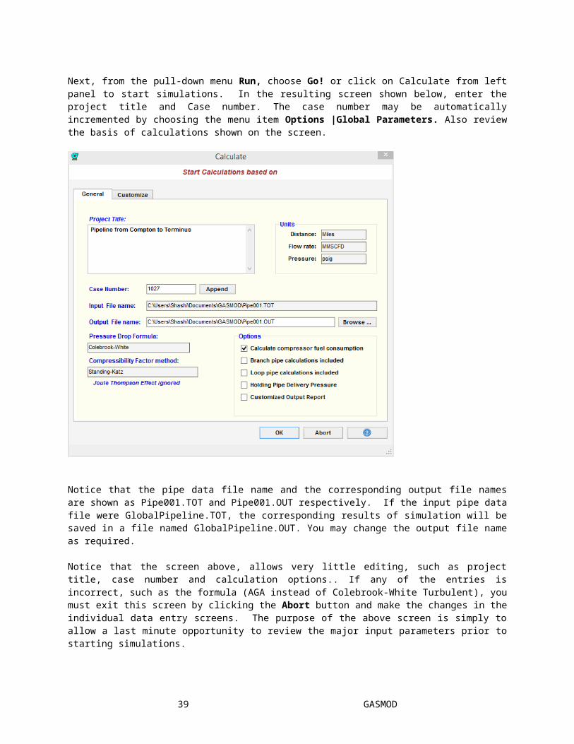
Next, from the pull-down menu Run, choose Go! or click on Calculate from left panel to start simulations. In the resulting screen shown below, enter the project title and Case number. The case number may be automatically incremented by choosing the menu item Options |Global Parameters. Also review the basis of calculations shown on the screen.

Notice that the pipe data file name and the corresponding output file names are shown as Pipe001.TOT and Pipe001.OUT respectively. If the input pipe data file were GlobalPipeline.TOT, the corresponding results of simulation will be saved in a file named GlobalPipeline.OUT. You may change the output file name as required.

Notice that the screen above, allows very little editing, such as project title, case number and calculation options.. If any of the entries is incorrect, such as the formula (AGA instead of Colebrook-White Turbulent), you must exit this screen by clicking the Abort button and make the changes in the individual data entry screens. The purpose of the above screen is simply to allow a last minute opportunity to review the major input parameters prior to starting simulations.

30 GASMOD

By clicking the Customize tab in the above screen, you may create a customized output report by selecting portions of the simulated results in any order desired as shown next.

It can be seen that the various sections of the output report can be customized as needed by choosing the elements and their order as shown.

The default output will consist of all sections of output as shown in the Sample Report section of this User Manual.

Click the OK button after entering all data to start calculations.

31 GASMOD

After a pause, varying from several seconds to a few minutes depending on the computer, the results of the simulation are displayed on the screen in a scrollable window similar to the one shown below:

The calculated results are also automatically saved on disk in a text file named Pipe001.OUT. Click the Print button to generate a hard copy of the results, if a printer is connected and turned on. You may also highlight the entire output using the mouse and copy the output to the Windows clipboard using the CTRL-C keys. You may then paste the clipboard contents into an application such as Microsoft Word, for inclusion in a report. You may also export the output report to the Windows Notepad or Excel by clicking the Export… button. To rename the output report click the Rename file… button. To plot a hydraulic pressure gradient showing the pressures along the pipeline, click the Hydraulic Gradient button. After viewing the results of the calculations on the screen, click the Close button or press the Esc key.

The printed output is included at the end of this User Manual under the heading Sample Output, along with additional results of other sample problems.

32 GASMOD

4.3 File Format for Pipe Data File The sample pipe data file used with GASMOD is named Pipe001.TOT and is displayed in a spreadsheet when you use the pull down menu File |Open to open the specified data file. The format of the file as it shows up on the spreadsheet is self-explanatory. As the cursor is moved from one cell to the next, the status bar at the bottom of the screen displays a short description of what is expected in each cell.

This spreadsheet has features similar to Microsoft Excel. You may select or highlight and delete rows, insert rows, cut, copy and paste data between cells for common editing tasks. Use the Edit/Copy/Paste options to import and export between an Excel spreadsheet and the GASMOD spreadsheet. Several short cut keys such as CTRL-C for Copy and CTRL-X for Cut are also implemented. To insert or delete rows CTRL-I and CTRL-D may be used.

Creating a pipe data file

Since the pipeline data file is the most important data needed for running GASMOD, it is appropriate to describe the creation and editing of the data file.

The simulation results are automatically saved under the same name as the data file, except the file extension is OUT. Thus, if the input pipe data file is named MyPipeline.TOT, then the results of the calculations are stored in the file MyPipeline.OUT in the same folder. The data file is created in a spreadsheet style editor. When saved to disk, the format is a special ASCII text format. Beginning with GASMOD Version 6.0, all pipeline model files that are created will be located in the My Documents\GASMOD folder.

DO NOT edit this file using a text editor or Word Processor. To edit the input data file, use only the GASMOD spreadsheet editor described here.

Note: A maximum of 1000 points (nodes) are allowed in the pipe data file.

The screen shot below shows the spreadsheet editor with the Pipe001.TOT file information.

33 GASMOD

Each column in the spreadsheet is for a specific data for the pipeline. Each row represents a specific location along the pipeline. As the cursor (arrow) keys are moved around in the spreadsheet cells, the status bar at the bottom of the screen briefly describes the information to be entered in each cell. After each data entry, move to the next cell by using the arrow keys or the tab key. The first column is for the distance measured from the origin of the pipeline, such as mile post. Each subsequent location of the pipeline is measured from the beginning of the pipeline and hence the first column is the cumulative length of each point (node) on the pipeline measured from the beginning, also designated as mile post location (m.p.).

It is not necessary to start the pipeline mile post at 0.0. For example, a pipeline, 220 miles long may be defined as starting at m.p. 525.0 and terminating at m.p. 745.0

Note: Unlike other hydraulic simulation models, the pipeline distances are cumulative and not pipe segment lengths.

34 GASMOD

The second column is for the elevation of the pipe at that mile post location, measured above some datum, such as sea level. The third and fourth columns represent the pipe outside diameter and pipe wall thickness at this location. The pipe diameter and wall thickness entered at a specific milepost location represent those for the pipe segment downstream of that milepost location. Thus, if the first two milepost locations are 0.0 and 48.0, the diameter and wall thickness entered at 0.0 milepost are for the pipe segment from 0.0 to the 48.0 location. The diameter and wall thickness entered at milepost 48.0 are for the next pipe segment starting at milepost 48.0. Accordingly, for the very last milepost location (the last data row of the spreadsheet), the diameter and wall thickness entered should be a duplicate of the immediately previous location, since there is no pipe segment downstream of the last milepost.

The next column is for the absolute roughness of the pipe interior. For new steel pipe, a roughness value of 0.0007 inches (700 micro inches) is generally used. If the pipe is internally coated, a lower value such as 200-300 micro inches may be used. In SI units a default pipe roughness of 0.02 mm may be used for bare pipe and 0.005 mm for internally coated pipe.

The next column entry is the Maximum Allowable Operating Pressure (MAOP) for the pipe at that milepost location and the final column is for the name of the pipe node location.

Also displayed below the spreadsheet are input fields for Inlet pressure, Delivery pressure, Minimum pressure and a check box for choosing Hold Delivery Pressure option. If the latter option is selected, calculations will be performed to ensure that the specified pipe delivery pressure at the end of the pipeline is attained. Otherwise, the delivery pressure will be calculated by holding constant the compressor station discharge pressure at the last compressor station. In most cases, it is desirable to have a contract delivery pressure at the pipeline terminus. Therefore this option is usually checked.

35 GASMOD

4.4 Pipe Branches The menu item Branch is used for specifying pipe branches and pipe loops along the pipeline. The branch pipe data file has a format similar to the main pipe data file and needs to be created separately first as described in File Format for Pipe Data in section 4.3.

If you are creating a new branch on an existing mainline, first create the pipe branch from the main pipe data screen similar to how you would create the main pipe file. For example suppose you have already created the main pipe data known as ABCPipeline and you now want to create an outgoing pipe branch (named BranchOut) on this pipeline that extends from milepost 45 on the main pipeline to a delivery point 30 miles away. First, close the main pipe data file (ABCPipeline) and create the branch pipe by clicking on File |New menu. This is the same as clicking the Pipeline button on the left panel. This will open up a blank spreadsheet. Enter the mileposts, elevation etc for the branch pipe as you would for the main pipeline and save the file under the name BranchOut. Note that the elevation at the junction point for the branch and the mainline point, must match. Thus if the elevations at mp 45 on the mainline (ABCPipeline), where branch pipe BranchOut is connected is 250 ft, the elevation at the first milepost of BranchOut must also be 250 ft. The mp numbering on the BranchOut file can start at 0.00 and extend to mp 30 at D

36 GASMOD

Main Pipeline

A

B

C

Q1

E

BranchOut

Branch2 Q2

m.p. 45Elev 250' m.p. 250

F

QD

Also create the thermal conductivity data for the branch by selecting the Conductivity menu. Next, create the gas flow data for the branch by clicking on the Gas Flow menu. Note that the gas flow leaving the mainline at milepost 45 (Q1) in this example must match the gas flow entering the branch pipe BranchOut.

Finally, close the branch data file and open the main pipeline ABCPipeline. Go to the Branch menu and enter the pertinent data for the branch under the tab titled Branches. You will specify the distance, type, branch filename etc., as described next

37 GASMOD

The menu item Branch is used for entering branch pipe and pipe loop information, as shown below:

In the screen above, the first column for distance represents the location (milepost) along the main pipeline where a branch pipe is connected.

An outgoing branch off the main pipeline (at mp 45 above) is designated by choosing OUT under the column Type. A pipe branch that delivers product into the main pipeline is called an incoming branch and therefore must be designated as IN under the Type column.

In the third column enter name of the branch pipe file name. Right-click on the branch file name above to view the branch pipe data, gas flow data or conductivity data. Pressing F3 shows all available branch data files.

38 GASMOD

For an outgoing branch pipe you must specify the delivery pressure required at the end of the branch when creating the branch data file

For an incoming branch pipe, you must indicate the starting temperature at the beginning of the branch when creating the data file. The starting pressure at the beginning of the incoming branch will be calculated by the program such that the required pressure at the junction of the mainline is matched.

An important aspect of branch pipe format is as follows. An outgoing branch pipe will have distances increasing in the direction of flow (outward) and the starting elevation of the branch pipe should be the same as that of the main pipeline at the connection point. Similarly, for an incoming pipe branch, the distances are measured from the start of the pipe branch in the direction of flow, towards the main pipeline. The elevation of the pipe branch at the connecting point must match that of the main pipeline at the junction.

No Compressor stations are allowed on the branch piping in this version of the program. Enter all data and click on Save when done. To get help, click the Help button

Note: The maximum number of data points (nodes) allowed on a branch pipe data file is 500 points. There can be a maximum of 50 branches off the mainline.

Hydraulic calculations are first performed along the main pipeline. For an outgoing branch the pressure at the main pipeline take off point is used to calculate the downstream pressures along each branch pipe. If the main pipeline flow rate at the branch takeoff point does not match the flow rate specified in the branch pipe data file, a warning message is displayed prior to calculations.

Similarly, for an incoming branch pipe, the flow rate into the main pipeline should match the combined flow rate in the last segment of the branch pipe connecting to the main line. The program calculates the pressure at the beginning of the incoming branch pipe needed to match the junction pressure at the main pipeline connection.

39 GASMOD

4.5 Pipe Loops The menu item Branch is also used for specifying pipe loops along the pipeline. The pipe loop data file has a format similar to the main pipe data file and needs to be created separately first, similar to the branch pipes.

If you are creating a new loop on an existing mainline, first create the pipe loop from the main pipe data screen similar to how you would create the main pipe file. For example suppose you have already created the main pipe data known as ABCPipeline and you now want to create a pipe loop (named Loop1) on this pipeline that extends from milepost 10 to milepost 25. Close the main pipe data file (ABCPipeline) and create the loop by clicking on File/New menu. This will open up a blank spreadsheet. Enter the mileposts, elevation etc for the pipe loop as you would for the main pipeline and save the file under the name Loop1. Also create the thermal conductivity data for the loop by selecting the Conductivity menu. Finally, close the loop data file and open the main pipeline ABCPipeline. Go to the Branch menu and enter the pertinent data for the loop under the tab titled Loops. You will specify the starting mile post and ending milepost along with the name of the pipe loop (Loop1). It must be noted that the starting mile post and ending milepost are measured along the main pipeline. For example Loop1 may be 20 miles long, whereas the starting mile post and ending milepost may be 10 and 25 miles respectively on the mainline. Also the elevations at the junction points for the loop and the mainline must match. Thus, if the elevations at mp 10 and mp 25 on the mainline (ABCPipeline) are 100 ft and 200 ft respectively, in the loop file (Loop1), the first milepost and last milepost should have elevations of 100 ft and 200 ft respectively.

A

B

m.p. 10

D

m.p. 25

C

Loop1

Main line

40 GASMOD

Similar to branch piping, you may view the pipe loop data file by right clicking on the file name.

Caution:

1. An important aspect of looped pipelines is that the loops must be contained entirely within a segment of the main pipeline between two Compressor stations. This means that the loop start and loop end locations may be 10.0 and 30.0 for a pipeline with Compressor stations at locations 0.00 and 50.0. However, for this pipeline the loop may not start at 10.0 and end at 60.0

2. The start and end of loops should not be at a location where delivery or injection occurs.

3. Loops cannot start at the beginning milepost or end at the last milepost of the pipeline. Ensure that a small length (such as 0.01 miles) of main pipe precedes the start of the loop and similarly a small section of pipe follows the end of the looped pipe segment.

If there is a pipe loop upstream and downstream of a compressor station as shown in the sketch below, the loops have to be split so that the entire loop is contained between the compressor stations, resulting in two loops as shown below. Otherwise calculations will be incorrect, and sometimes the program may hang up.

4.6 Building pipeline model graphically

41 GASMOD

Wrong

Correct

The pipeline model may be created graphically using a drag and drop approach, via a Graphic model builder known as PipeGraph-G. In this method, objects such as pipe segments, valves, compressor stations and other devices may be selected from a toolbox and dropped on a drawing area. These objects can be connected with pipe segments to form the pipeline system. The properties of each object may be defined by double-clicking on them and entering data in the screen that is displayed. A video tutorial is available at SYSTEK’s website that explains how the pipeline model can be created graphically. Once the graphic model is created, the GASMOD input file is automatically created.

Upon choosing the Graphic model option, from the GASMOD left panel, the PipeGraph-G screen is displayed as below:

The Help menu displays a General Help screen explaining the features of PipeGraph-G as shown below:

42 GASMOD

Create the pipeline by choosing objects from the toolbox on the left and dropping them on the canvas or drawing are as shown.

43 GASMOD

In the example shown a pressure object (Pressure0), three pipe segments (Pipe0, Pipe1 and Pipe2), a compressor station object and a pressure regulator are used. Double-clicking an object displays the properties screen for entering data pertaining to that object. In this case there is a pressure of 1000 psi at the beginning of the pipeline (from a connection to another pipeline).

44 GASMOD

Since there must be a gas flow at the inlet of the pipeline, a flow object (Q) is dropped on the pressure object. This results in the P icon having a small Q object at its bottom right hand corner. Double-clicking the pressure object displays the properties screen again for entering data on the gas flow rate as shown.

Similarly, the properties of each pipe segment, compressor station and the pressure regulator are specified by double-clicking each object and entering the properties as indicated in the subsequent screens.

45 GASMOD

Pipe segment data:

Compressor station data:

46 GASMOD

Pressure regulator data:

47 GASMOD

After entering all properties, the project file may be saved by choosing File| Save As option. Project files created have a file extension of .plproj. A TOT file for use with GASMOD is automatically created in the right format. Alternatively, from the Options menu choosing Create TOT file will also create the GASMOD TOT file for this project.

Quitting PipeGraph-G will revert to the GASMOD screen with the File| Open dialog box for choosing the TOT file as shown below

48 GASMOD

4.7 Locating Compressor StationsWhen designing a new pipeline system, it is necessary to roughly determine the locations of compressor station for hydraulic balance. Normally, trial locations along the pipeline are selected and the hydraulics simulated. After making an initial hydraulic run, these compressor station locations are then adjusted to balance the horsepower required at each station or to ensure approximately same discharge pressures. This process will generally involve making several runs until the discharge pressures and horsepower are balanced. However, GASMOD provides an option to quickly determine the approximate compressor station locations for hydraulic balance as follows.

From the menu Station, choose Locate Compressor Stations and the following screen is displayed:

49 GASMOD

After data input, click Calculate and the program will ignore the current compressor sites and calculate the number and approximate locations of the compressor stations required for the specified gas flow rate, based upon a maximum discharge pressure and compression ratio.

The locations thus determined may be inserted in the pipe data file and the simulation hydraulics re-run. It must be noted that these station locations are approximate since calculations are based on isothermal flow and ignores any intermediate gas deliveries or injections.

50 GASMOD

4.8 Quick Start OptionThe Quick Start option (under the Options menu) allows you to quickly build a pipeline model by specifying some basic data on the pipeline, gas flow rate and gas properties. Under the Options menu, selecting the Quick Start item displays the following screen:

Click the OK button and the Units screen is displayed for choosing the calculation units. Next the following Quick Start data entry screen is displayed:

51 GASMOD

The Quick Start screen on the preceding page shows a typical gas pipeline with some basic pipe and gas data already filled in. Make changes as needed for your specific problem. For example, suppose you want to quickly create a model of a 100 mile 20 inch pipeline with two compressor stations to simulate a gas flow rate of 200 MMSCFD, with compressor suction and discharge pressures of 800 and 1400 psig respectively. Enter the data as shown in the previous screen and click OK.

The TOT file will be automatically created based on the data you specified as well as some additional default data and displayed in the pipeline spreadsheet as shown below

You may then examine the resulting pipe data screen, the compressor station and gas flow rate screens and make any changes desired. The model can then be run to simulate the required flow rate.

52 GASMOD

4.9 Quick Pressure DropClicking the icon on the toolbar with the letter Q, the “Quick Pressure Drop” option screen shown below opens up.

This is for quick calculation of isothermal pressure drop in a pipe segment. For a given flow rate, pipe diameter, pipe length, specific gravity and viscosity, the Quick Pressure Drop screen is used to calculate the inlet or outlet pressure, given one of the two pressures. If the outlet pressure is specified, the inlet pressure is calculated and vice versa. Of the three variables: flow rate, inlet pressure and outlet pressure, two items may be specified and the third one calculated. Leave the item to be calculated, blank.

53 GASMOD

To select units of calculations, Click the Units… button and choose English or SI-Metric.

You can select a gas composition from the database included, by clicking the Gas… button. The specific gravity and viscosity of the gas chosen will be calculated and inserted in the respective fields.

The gas compressibility option (Standing-Katz, CNGA, etc) may be chosen from the drop down combo box.

Choose the pressure drop formula (such as AGA turbulent, Colebrook-White etc.) to be used.

After entering all data, click Calculate to determine the inlet or outlet pressure, or the flow rate.

Clicking the More… button will display additional results of calculations, such as the velocities, Reynolds number, transmission factor, friction factor and the compressibility factor as shown below:

The Quick Pressure Drop calculation is completely independent of the main program, except it shares two global parameters, namely, the units of calculation and formula used. If either of these is changed in the Quick Pressure Drop screen, it affects the main pipe data file as well. Therefore, when returning to the main program to run a pipe data file verify the units of calculation and formula used, prior to simulating the model.

54 GASMOD

4.10 Cost calculations The toolbar icon with a $ sign is used for quick estimation of pipeline capital costs, annual operating costs and the annual cost of service and transportation tariff. On clicking this icon the following screen is displayed:

The above screen displays the tabs for Capital cost, Operating cost and Tariff. Most of the data in the various fields have already been filled in as a result of the hydraulic calculations. Make changes as needed and click the Calculate button to recalculate the costs.

In the Capital Cost screen, for the current pipeline system, the pipe tonnage, number of compressor stations, estimated main line valve installations, meter stations and miscellaneous costs are shown. In English units, Pipe material cost is based on $1000 per ton, compressor station cost is based on $1500 per HP installed, $50,000 per mainline valve installation, etc. Any of these values can be edited and the capital cost re-calculated by clicking the Calculate button. Note that the costs shown in this screen include only the main pipeline. Cost of pipe branches and loops, if any, are not shown.

The Miscellaneous (rows) cost is shown as a percentage of the first four line items (pipeline, compressor etc.). The indirect costs such as Right of Way (ROW), Environmental etc. are also represented as a percentage of the first five line items. These percentages may be changed as needed. The Contingency and AFUDC are included as a percentage of the subtotal of all items above the Contingency line. Click the Help button for more information on the basis of calculation. To obtain a hard copy of the capital costs, click the Print button.

55 GASMOD

Similar to the Capital cost, the tab titled as Operating cost will display spreadsheets showing the compressor stations, HP calculated, gas fuel consumption rate, gas fuel cost in $/MCF, etc. as shown below. Gas turbine drivers are assumed at the compressor sites.

The lower spreadsheet includes other annual costs such as Operation & Maintenance (O&M), Payroll etc. These descriptions can be changed by clicking the Customize button. Make changes as necessary to the Description as well as the $/Year amounts and click the Calculate button to obtain the total annual operating cost. The total annual costs include the fuel costs and other annual costs.

Click the Tariff tab to go to the Tariff screen as shown on the next page.

56 GASMOD

The transportation tariff and the Annual cost of service can be calculated from the results of the previous cost screens. The Tariff screen is shown below:

In the above screen, the Capital cost and Annual operating costs from the previous tabs have been transferred to this tab. The pipeline input flow rate has also been filled in.

You may change any or all the financial parameters such as interest rate, rate of return (ROR), tax rate, financing option (debt/equity ratio), etc. and perform “what if” analyses. Click the Calculate button to calculate the Annual cost of service and the transportation tariff, such as $/MCF. Click the Print button to produce a hard copy of the results. Click the Close button or the Escape key to close this screen. See the Reference section for the basis of these financial calculations.

57 GASMOD

5. ReferenceThis section provides an explanation of formulas and variable names used.

5.1 Hydraulic FormulasThe following symbols are used in the equations below:

Q - Gas flow rate - standard ft3/day (SCFD) (m3/day in SI units) P1 - Upstream Pressure, psia. (kPa in SI units)P2 - Downstream Pressure, psia. (kPa in SI units)Pavg - Average Pressure, psia. (kPa in SI units)Pb - Base pressure, psia. (kPa in SI units)Tb - Base temperature, deg R (K in SI units)Tf - Average gas flow temperature, deg R (K in SI units)L, L1, L2 - Pipe segment length, miles (km in SI units)L e - Equivalent length, miles (km in SI units)e - Base of natural logarithms, e = 2.71828….j - Parameter that depends on s for each pipe segment, dimensionlessG - Gas gravity (Air = 1.00) - Gas viscosity, lb/ft-sec (Poise in SI units) E - Pipe efficiency, percent/100D - Pipe inside diameter, inches (mm in SI units)Z - Gas compressibility factor, dimensionlessF - Transmission factor f - Darcy friction factorFt

- Von Karman smooth pipe transmission factorDf - Pipe drag factors - Elevation adjustment factor, dimensionless E1 - Upstream pipe elevations, ft (m in SI units) E2 - Downstream pipe elevations, ft (m in SI units)k - Absolute pipe roughness, inches (mm in SI units)R - Reynolds number, dimensionless HP - Compressor horsepower - Ratio of specific heats of gas, dimensionless

Ts - Compressor gas suction temperature, deg R (K in SI units)Ps - Compressor suction pressure, psia (kPa in SI units)Pd - Compressor discharge pressure, psia (kPa in SI units) Zs - Compressibility of gas at suction conditions, dimensionless Zd - Compressibility of gas at discharge conditions, dimensionless a - Compressor adiabatic (isentropic) efficiency, decimal value

58 GASMOD

Reynolds number of flow:

R=0 .0004775×Pb

Tb×GQ

μD

Laminar Flow:Laminar Flow:

Friction factorFriction factorf=64

R for R <= 2000 for R <= 2000

Average Pressure:

Pavg =

23 (P1+P2−

P1×P2

P1+P2)

Compressibility factor:

The compressibility factor varies with the Gas composition, temperature and pressure. GASMOD calculates the compressibility factor using one of the following three methods:

1. Standing-Katz Method2. CNGA Method3. AGA NX19 Method

1. The Standing-Katz Method is based on charts published in the Transactions of AIME, 146, 144 in January 1941.

2. CNGA Method is based on the following equation:

Z= 1

[1+( Pavg344400 (10 )1 .785G

T f3. 825 )]

for Pavg > 100

Z = 1.00 for Pavg <= 100

Note that Pavg in the above equation is the average pipe pressure in psig

59 GASMOD

3. AGA NX19 method uses the approach outlined in AGA-IGT, Report No. 10. This correlation is valid for temperatures between 30 degF and 120 degF and for pressures up to 1,380 psig. It produces an error of less than 0.03 percent in this range of temperatures and pressures. Beyond this range the discrepancy can be up to 0.07 percent.

For details of other methods of compressibility calculations refer to American Gas Association publication Report No. 8, Second Edition, November 1992.

Elevation Adjustment:

s=0 .0375G( E1−E2

T f Z )

AGA Equation:

Fully Turbulent F=4 Log10( 3 .7D

k )

Partially TurbulentF=4 Df Log10( R

1.4125 F t ) and

F t=4 Log10( RF t )−0 .6

Colebrook-White Equation:

Friction factor

1√ f

=−2 Log10( k3 .7 D

+ 2.51R√ f )

for Turbulent flow R > 2000

Modified Colebrook-White Equation:

1√ f

=−2 Log10( k3 .7 D

+ 2. 825R√ f )

For turbulent flow R > 2000

F=−4 Log10( k3 .7 D

+1 .4125 FR )

For turbulent flow R > 2000

60 GASMOD

Darcy friction factor and Transmission factor:

f= 4F2

F= 2√ f

General Flow Equation:

Q=38 . 77 F(T b

Pb )( P12−es P2

2

GT f LeZ )0. 5

D2 .5

…………….. English Units

Q=5 . 747×10−4 F (T b

Pb )(P12−esP2

2

GT f LeZ )0 .5

D2. 5

…………….. SI Units

Le = j1L1 + j2L2 es1 + j3L3 es2 + …….

j= es−1s

IGT Equation:

Q=136 . 9 E(T b

Pb )( P12−esP2

2

G0. 8T f Leμ0.2 )

0. 555

D2. 667

……………….. English Units

Q=1 . 2822×10−3 E (Tb

Pb )( P12−esP2

2

G0 . 8T f Le μ0 .2 )

0 .555

D2 .667

……………….. SI Units

61 GASMOD

Panhandle A:

Q=435 .87 E (Tb

Pb )1 .0788

( P12−esP2

2

G0 .8539T f LZ )0.5394

D2 .6182

……………….. English Units

Q=4 . 5965×10−3 E(T b

Pb )1. 0788

( P12−esP2

2

G0 . 8539T f LZ )0 .5394

D2. 6182

……………….. SI Units

Panhandle B:

Q=737 E (Tb

Pb )1 . 02

( P12−esP2

2

G0 . 961T f LZ )0. 51

D2 .53

……………….. English Units

Q=1 . 002×10−2E (Tb

Pb )1 .02

( P12−esP2

2

G0 .961T f LZ )0.51

D2 .53

……………….. SI Units

Weymouth:

Q=433 .5 E(T b

Pb )( P12−esP2

2

GT f LZ )0.5

D2 .667

……………….. English Units

Q=3 . 7435×10−3 E(T b

Pb )(P12−esP2

2

GT f LZ )0 . 5

D2. 667

……………….. SI Units

Compressor Horsepower:

HP=8 . 57×10−8( γγ−1 )QT s( Zs+Zd

2 )( 1ηa )[( Pd

Ps )γ−1γ −1]

……………….. English Units

Power=4 . 0639×10−6( γγ−1 )QT s (Zs+Zd

2 )( 1ηa) [(Pd

Ps )γ−1γ −1]

……………….. SI Units

62 GASMOD

5.2 Cost FormulasThe following symbols are used in the equations below:

Capital - Total capital employed, $Debt - Percentage of capital that is borrowed, %

Cap1 - Portion of total capital that is borrowed (debt capital), $Cap2 - Portion of total capital that is equity (equity capital), $

Tax - Annual corporate tax rate, %ROR - Annual Rate of Return desired, %IntRate - Interest rate per year on borrowed capital, %CostSvc - Cost of Service per year, $/year

IntCost - Interest cost per year, $/yearEqtyCost - Equity cost per year, $/yearOMCost - Annual Operating and Maintenance cost, $/yrOtherCost - Other annual costs (G&A, etc.), $/yr

Life - Project life in yearsDepr - Annual depreciation cost (linear with zero salvage value), $/yr

Vol - Daily throughput volume, SCFDTariff - Transportation tariff, $/MCF

Capital split between debt and equity:

Debt capital Cap 1=Capital×Debt

100

Equity capital Cap 2=Capital−Cap1

Calculate interest payment on debt:

Interest cost per year IntCost=Cap1×IntRate

100

63 GASMOD

Calculate earnings on equity required at ROR:

Equity cost per yearEqtyCost=Cap2×(ROR /100 )

1−Tax /100

Calculate Depreciation:

Straight line depreciation per year

Depr=CapitalLife

Total cost of service:

CostSvc = IntCost + EqtyCost + Depr + OMCost + OtherCost

Tariff=CostSvc×1000365×Vol $/MCF ($/m3 in SI units)

Based on heating value HV in Btu/ft3 (GJ/m3 in SI units) the tariff is as follows:

Tariff= CostSvc×106

365×Vol×HV $/MMBtu ($/GJ in SI units)

64 GASMOD

6. TroubleshootingGASMOD is a powerful steady state hydraulic simulation program for gas pipelines under thermal flow. The program is very user friendly and online HELP is available for most data entry screens. The program has extensive error checking features. However, there is always a possibility that some extraneous or invalid data was entered and the program may hang up. In such cases, try quitting the program by using the Exit icon on the toolbar. If this does not work, you may have to re-boot the computer and start over. Another alternative is to go to the Windows Task list and click on End Task to quit GASMOD. Re-booting may be necessary as a last resort.

If you cannot get GASMOD to run properly even after following the steps outlined in the Getting Started section of this manual, please check the following before you call Technical Support.

6.1 Error Messages:Here are some errors that you may encounter while running GASMOD:

1. Divide by zero errorThis is generally due to some data input value that is zero. Check all input data for zero values. The compressor efficiencies, specific gravity, viscosity are usually suspect.

2. Illegal Function callThis is generally due to some illegal mathematical operation such as trying to extract the square root of a negative value. Ensure that there are no inadmissible negative values, such as a negative value for viscosity or specific gravity.

3. File not foundA common error when a file specified cannot be located on the hard disk or does not exist. When specifying data files, make sure the file is present in the sub-directory or folder containing GASMOD. Otherwise, ensure that the file name is typed in correctly, including the full path.

4. Input past end of fileThis happens when the program reads a data file and looks for more information than present in the file. For example, it tries to read 10 sets of pipe data (distance, elevation, etc.) points from a data file where only 9 sets of data exist. You may load the data file into an ASCII text editor and review the file for errors.

5. Overflow This is similar to the first two errors and happens when the program attempts to perform some illegal mathematical operation. Check all data for zero values that might cause such a condition. In particular, check all thermal conductivity and heat transfer data.

65 GASMOD

7. Technical SupportPlease read the Troubleshooting section of this manual before you call us for technical support. Also, you may check the FAQ section at the SYSTEK web site for answers to most commonly asked questions.

Free Technical Support is provided for registered users of this software for a period of one year from the initial purchase date. After that period, Technical Support can be provided only if an annual software maintenance and support plan has been purchased. Contact SYSTEK for details.

7.1 How to contact usIn order to facilitate quick response, please have your disk serial number and program version available when you call us.

How to contact us:

You may contact SYSTEK in any of the following ways:

Phone/Fax: (928) 453-9587

E-mail: support@systek.us

Web site: www.systek.us

66 GASMOD

8. Sample Reports

67 GASMOD

Sample Problem –1 (English Units)This is the same as the sample problem discussed in the Tutorial section of this manual.

An 18-inch/16-inch diameter, 420 mile long buried pipeline defined below is used to transport 150 MMSCFD of natural gas from Compton to the delivery terminus at Harvey. There are three compressor stations located at Compton, Dimpton and Plimpton, with gas turbine driven centrifugal compressors. The pipeline is not insulated and the maximum pipeline temperature is limited to 140 deg F due to the material of the pipe external coating. The maximum allowable operating pressure (MAOP) is 1440 psig. Determine the temperature and pressure profile and horsepower required at each compressor station.

68 GASMOD

The pipeline profile is defined below:

Distance Elevation Pipe dia. Wall thick. Roughness(miles) (ft) (in) (in) (in)

0.0 620 18.00 .375 0.00070045 620 18.00 .375 0.00070048 980 18.00 .375 0.00070085 1285 16.00 .375 0.000700160 1500 16.00 .375 0.000700200 2280 16.00 .375 0.000700238 950 16.00 .375 0.000700250 891 16.00 .375 0.000700295 670 16.00 .375 0.000700305 650 16.00 .375 0.000700310 500 16.00 .375 0.000700320 420 16.00 .375 0.000700330 380 16.00 .375 0.000700380 280 16.00 .375 0.000700420 500 16.00 .375 0.000700

Gas specific heat (K) ratio : 1.26Maximum Gas velocity : 50 ft/secPipeline efficiency : 1.00Base temperature : 60 deg FBase pressure : 14.70 psia.Pressure drop formula : Colebrook-WhiteCompressibility factor : Standing-KatzPolytropic index : 1.3

A flow rate of 150 MMSCFD enters the pipeline at Compton (milepost 0.0) and at an intermediate location named Doodle (milepost 85), a delivery of 20 MMSCFD is made. Additionally an injection of 10 MMSCFD is made at Kreepers (milepost 238). The resulting flow then continues to the end of the pipeline. Gas inlet temperature is 70 deg F at both locations.

Inlet Gas specific gravity (air = 1.00) : 0.600Inlet Gas Viscosity : 0.000008 lb/ft-sec

The compressor stations are as follows:

Compressor Location Discharge Press. station (miles) (psig) Compton 0.00 1400Dimpton 160.0 1400Plimpton 295.0 1400

69 GASMOD

The installed HP at each compressor stations is 5,000 HP

Origin suction pressure : 800 psig.Pipeline delivery pressure : 500 psig.Minimum pipe pressure : 400 psig.Station suction loss : 5 psigStation discharge loss : 10 psigCompressor adiabatic efficiency : 85 %Compressor mechanical efficiency : 98 %Fuel consumption : 0.2 MCF/day/HP

Pipe burial depth : 36 inchesPipe thermal conductivity : 29 Btu/hr/ft/deg FSoil thermal conductivity : 0.800 Btu/hr/ft/deg FAmbient soil temperature : 65 deg FOrigin suction temperature : 70 deg F

70 GASMOD

************ GASMOD - GAS PIPELINE HYDRAULIC SIMULATION *********************** Version 7.00 ************DATE: 9/3/2015 TIME: 08:47:14 PROJECT DESCRIPTION:Problem 1Pipeline from Compton to Harvey18"/16" pipeline - 420 miles longCase Number: 1011 Pipeline data file: C:\Users\Shashi\Documents\GASMOD\ProblemFiles\Problem1.TOT

Pressure drop formula: Colebrook-White Pipeline efficiency: 1.00 Compressibility Factor Method: Standing-Katz

Inlet Gas Gravity (Air=1.0): 0.60000 Inlet Gas Viscosity: 0.0000080 lb/ft-sec Gas specific heat ratio: 1.29 Polytropic compression index: 1.30

****** Calculations Based on Specified Thermal Conductivities of Pipe, Soil and Insulation ******

Base temperature: 60.00 degF Base pressure: 14.70 psia

Origin suction temperature: 70.00 degF Origin suction pressure: 800.00 psig Pipeline Terminus Delivery pressure: 933.52 psig Minimum pressure: 400.0 psig Maximum gas velocity: 50.00 ft/sec

Inlet Flow rate: 150.00 MMSCFD Outlet Flow rate: 138.06 MMSCFD

CALCULATION OPTIONS:Polytropic compression considered: YES Branch pipe calculations: NO Loop pipe calculations: NO Compressor Fuel Calculated: YES Joule Thompson effect included: NO Customized Output: NO

ALL PRESSURES ARE GAUGE PRESSURES, UNLESS OTHERWISE SPECIFED AS ABSOLUTE PRESSURES

**************** PIPELINE PROFILE DATA ***********

Distance Elevation Diameter Thickness Roughness miles ft in in in

0.00 620.00 18.000 0.380 0.000700 45.00 620.00 18.000 0.380 0.000700 48.00 980.00 18.000 0.380 0.000700 85.00 1,285.00 16.000 0.380 0.000700 160.00 1,500.00 16.000 0.380 0.000700 200.00 2,280.00 16.000 0.380 0.000700 238.00 950.00 16.000 0.380 0.000700 250.00 891.00 16.000 0.380 0.000700 295.00 670.00 16.000 0.380 0.000700 305.00 650.00 16.000 0.380 0.000700 310.00 500.00 16.000 0.380 0.000700

71 GASMOD

320.00 420.00 16.000 0.380 0.000700 330.00 380.00 16.000 0.380 0.000700 380.00 280.00 16.000 0.380 0.000700 420.00 500.00 16.000 0.380 0.000700

************** THERMAL CONDUCTIVITY AND INSULATION DATA ****************

Distance Cover Thermal Conductivity Insul.Thk Soil Temp miles in Btu/hr/ft/degF in degF Pipe Soil Insulation 0.000 36.000 29.000 0.800 0.020 0.000 65.00 45.000 36.000 29.000 0.800 0.020 0.000 65.00 48.000 36.000 29.000 0.800 0.020 0.000 65.00 85.000 36.000 29.000 0.800 0.020 0.000 65.00 160.000 36.000 29.000 0.800 0.020 0.000 65.00 200.000 36.000 29.000 0.800 0.020 0.000 65.00 238.000 36.000 29.000 0.800 0.020 0.000 65.00 250.000 36.000 29.000 0.800 0.020 0.000 65.00 295.000 36.000 29.000 0.800 0.020 0.000 65.00 305.000 36.000 29.000 0.800 0.020 0.000 65.00 310.000 36.000 29.000 0.800 0.020 0.000 65.00 320.000 36.000 29.000 0.800 0.020 0.000 65.00 330.000 36.000 29.000 0.800 0.020 0.000 65.00 380.000 36.000 29.000 0.800 0.020 0.000 65.00 420.000 36.000 29.000 0.800 0.020 0.000 65.00

**************** LOCATIONS AND FLOW RATES ****************

Location Distance Flow in/out Gravity Viscosity Pressure GasTemp. miles MMSCFD lb/ft-sec psig degF

Compton 0.00 150.0000 0.6000 0.00000800 800.00 70.00 85.00 -20.0000 0.6000 0.00000800 1,198.62 65.01 238.00 10.0000 0.6000 0.00000800 1,180.25 65.01 Harvey 420.00 -138.0636 0.6047 0.00000806 933.52 65.00

**************** COMPRESSOR STATION DATA **************

FLOW RATES, PRESSURES AND TEMPERATURES:

Name Flow Suct. Disch. Compr. Suct. Disch. Suct. Disch. MaxPipe Rate Press. Press. Ratio. Loss. Loss. Temp. Temp. Temp.

MMSCFD psig psig psia psia degF degF degF degF

Compton 149.13 795.00 1,410.00 1.7595 5.00 10.00 70.00 154.46 140.00Dimpton 128.59 912.35 1,410.00 1.5368 5.00 10.00 65.00 127.64 140.00Plimpton 138.06 943.60 1,410.00 1.4867 5.00 10.00 65.00 122.59 140.00

Gas Cooling required at compressor station: Compton to limit station discharge temperature to 140 degF

72 GASMOD

************* COMPRESSOR EFFICIENCY, HP AND FUEL USED ****************

Name Distance Compr Mech. Overall Horse Fuel Fuel Installed Effy. Effy. Effy. ower Factor Used HP miles % % % MCF/day/HP MMSCFD

Compton 0.00 85.00 98.00 83.30 4,329.48 0.2000 0.8659 5,000Dimpton 160.00 85.00 98.00 83.30 2,702.48 0.2000 0.5405 5,000Plimpton 295.00 85.00 98.00 83.30 2,650.19 0.2000 0.5300 5,000

Total Compressor Station Horsepower: 9,682.15 15,000

Total Fuel consumption: 1.9364 MMSCFD

************** REYNOLD'S NUMBER AND HEAT TRANSFER COEFFICIENT **************

Distance Reynold'sNum. FrictFactor Transmission HeatTransCoeff CompressibilityFactor miles (Darcy) Factor Btu/hr/ft²/degF (Standing-Katz)

0.000 8,763,167 0.0108 19.26 0.4624 0.8318 45.000 8,763,167 0.0108 19.26 0.4624 0.8192 48.000 8,763,167 0.0108 19.26 0.4624 0.8242 85.000 8,583,757 0.0110 19.08 0.4992 0.8444 160.000 8,583,757 0.0110 19.08 0.4992 0.8303 200.000 8,583,757 0.0110 19.08 0.4992 0.8255 238.000 9,248,473 0.0110 19.10 0.4993 0.8322 250.000 9,248,473 0.0110 19.10 0.4993 0.8455 295.000 9,248,473 0.0110 19.10 0.4993 0.8467 305.000 9,248,473 0.0110 19.10 0.4993 0.8283 310.000 9,248,473 0.0110 19.10 0.4993 0.8208 320.000 9,248,473 0.0110 19.10 0.4993 0.8173 330.000 9,248,473 0.0110 19.10 0.4993 0.8258 380.000 9,248,473 0.0110 19.10 0.4993 0.8466 420.000 9,248,473 0.0110 19.10 0.4993 0.8466

******************* PIPELINE TEMPERATURE AND PRESSURE PROFILE ********************

Distance Diameter Flow Velocity Press. GasTemp. SoilTemp. MAOP Location miles in MMSCFD ft/sec psig degF degF psig

0.00 18.000 149.1341 11.08 1400.00 140.00 65.00 1440.00 Compton 45.00 18.000 149.1341 11.86 1307.05 65.73 65.00 1440.00 48.00 18.000 149.1341 12.03 1288.53 65.52 65.00 1440.00 85.00 16.000 129.1341 14.32 1198.62 65.01 65.00 1440.00 160.00 16.000 129.1341 18.56 917.35 65.00 65.00 1440.00 Dimpton

160.00 16.000 128.5936 12.23 1400.00 127.64 65.00 1440.00 Dimpton 200.00 16.000 128.5936 13.62 1255.66 65.62 65.00 1440.00 238.00 16.000 138.5936 15.61 1180.25 65.01 65.00 1440.00 250.00 16.000 138.5936 16.20 1136.23 65.00 65.00 1440.00 295.00 16.000 138.5936 19.28 948.60 65.00 65.00 1440.00 Plimpton

295.00 16.000 138.0636 13.13 1400.00 122.59 65.00 1440.00 Plimpton 305.00 16.000 138.0636 13.45 1366.00 85.03 65.00 1440.00 310.00 16.000 138.0636 13.57 1354.61 76.49 65.00 1440.00 320.00 16.000 138.0636 13.87 1324.52 68.70 65.00 1440.00 330.00 16.000 138.0636 14.21 1292.67 66.18 65.00 1440.00 380.00 16.000 138.0636 16.46 1114.14 65.00 65.00 1440.00 420.00 16.000 138.0636 19.59 933.52 65.00 65.00 1440.00 Harvey

73 GASMOD

74 GASMOD

******************* LINE PACK VOLUMES AND PRESSURES ********************

Distance Pressure Line Pack miles psig million std.cu.ft

0.00 1400.00 0.0000 45.00 1307.05 38.9438 48.00 1288.53 2.7802 85.00 1198.62 32.6973 160.00 917.35 43.3324 200.00 1255.66 21.7444 238.00 1180.25 25.6117 250.00 1136.23 7.6398 295.00 948.60 25.4736 305.00 1366.00 5.7316 310.00 1354.61 3.6318 320.00 1324.52 7.3259 330.00 1292.67 7.2645 380.00 1114.14 33.2617 420.00 933.52 22.1823

Total line pack in main pipeline = 277.6210 million std.cu.ft

75 GASMOD

Sample Problem –2 (English Units)

This simulates a pipeline with two compressor stations and two pipe branches.A 12-inch/14-inch diameter, 180 mile long natural gas pipeline defined below is used to transport natural gas from Davis to the delivery terminus at Harvey. There are two compressor stations located at Davis (mp 0.0) and Frampton (mp 82.0) respectively. Each compressor station operates at a maximum discharge of 1200 psig. At Davis 100 MMSCFD (0.600 spgr) of gas enters the pipeline at 80F inlet temperature. An outgoing pipe branch (branch1 – NPS 8) is located at mp 25.0 that is used to deliver 30 MMSCFD of gas from the main pipeline to a delivery location 32 mile away. At mp 90.0 there is an incoming pipe branch (branch2) that is used to inject an additional volume of 50 MMSCFD gas (0.615 s.g.) into the main pipeline at 80F inlet temperature. The incoming branch pipe is NPS 10, 40 miles long. The pipelines are un-insulated and the maximum pipeline temperature is limited to 140 deg F. The soil temperature is assumed to be 60 deg F. Use an overall heat transfer coefficient (U factor) of 0.500 and the Colebrook-White equation for pressure drop. The pipe MAOP is 1440 psig. The base pressure and base temperature is 14.73 psia and 60F respectively. The delivery pressure at Harvey is 400 psi. Minimum pressure required is 300 psig. Origin suction pressure is 850 psig.Determine the temperature, pressure profile and horsepower required at each compressor station and the gas fuel consumption. Use the data on the report to create the pipeline and branches.

76 GASMOD

************ GASMOD - GAS PIPELINE HYDRAULIC SIMULATION *********************** Version 7.00 ************DATE: 9/3/2015 TIME: 08:57:08 PROJECT DESCRIPTION:Pipeline from Davis to HarveyCase Number: 1011 Pipeline data file: C:\Users\Shashi\Documents\GASMOD\ProblemFiles\Problem2.TOT

Pressure drop formula: Colebrook-White Pipeline efficiency: 1.00 Compressibility Factor Method: CNGA

Inlet Gas Gravity (Air=1.0): 0.60000 Inlet Gas Viscosity: 0.0000080 lb/ft-sec Gas specific heat ratio: 1.29 Polytropic compression index: 1.30

****** Calculations Based on Specified Thermal Conductivities of Pipe, Soil and Insulation ******

Base temperature: 60.00 degF Base pressure: 14.73 psia

Origin suction temperature: 80.00 degF Origin suction pressure: 850.00 psig Pipeline Terminus Delivery pressure: 446.92 psig Minimum pressure: 300.0 psig Maximum gas velocity: 50.00 ft/sec

Inlet Flow rate: 100.00 MMSCFD Outlet Flow rate: 119.36 MMSCFD

CALCULATION OPTIONS:Polytropic compression considered: YES Branch pipe calculations: YES Loop pipe calculations: NO Compressor Fuel Calculated: YES Joule Thompson effect included: NO Customized Output: NO

ALL PRESSURES ARE GAUGE PRESSURES, UNLESS OTHERWISE SPECIFED AS ABSOLUTE PRESSURES

**************** PIPELINE PROFILE DATA ***********

Distance Elevation Diameter Thickness Roughness miles ft in in in

0.00 220.00 12.750 0.250 0.000700 12.00 340.00 12.750 0.250 0.000700 25.00 450.00 12.750 0.250 0.000700 35.00 189.00 12.750 0.250 0.000700 82.00 225.00 12.750 0.250 0.000700 90.00 369.00 14.000 0.250 0.000700 112.00 412.00 14.000 0.250 0.000700 125.00 518.00 14.000 0.250 0.000700 152.00 786.00 14.000 0.250 0.000700 180.00 500.00 14.000 0.250 0.000700

77 GASMOD

************** THERMAL CONDUCTIVITY AND INSULATION DATA ****************

Distance Cover Thermal Conductivity Insul.Thk Soil Temp miles in Btu/hr/ft/degF in degF Pipe Soil Insulation 0.000 36.000 29.000 0.800 0.020 0.000 60.00 12.000 36.000 29.000 0.800 0.020 0.000 60.00 25.000 36.000 29.000 0.800 0.020 0.000 60.00 35.000 36.000 29.000 0.800 0.020 0.000 60.00 82.000 36.000 29.000 0.800 0.020 0.000 60.00 90.000 36.000 29.000 0.800 0.020 0.000 60.00 112.000 36.000 29.000 0.800 0.020 0.000 60.00 125.000 36.000 29.000 0.800 0.020 0.000 60.00 152.000 36.000 29.000 0.800 0.020 0.000 60.00 180.000 36.000 29.000 0.800 0.020 0.000 60.00

**************** LOCATIONS AND FLOW RATES ****************

Location Distance Flow in/out Gravity Viscosity Pressure GasTemp. miles MMSCFD lb/ft-sec psig degF

Davis 0.00 100.0000 0.6000 0.00000800 850.00 80.00 BranchOut 25.00 -30.0000 0.6000 0.00000800 1,024.48 62.06 BranchIn 90.00 50.0000 0.6150 0.00000800 1,170.47 75.28 Harvey 180.00 -119.3576 0.6077 0.00000802 446.92 60.00

**************** COMPRESSOR STATION DATA **************

FLOW RATES, PRESSURES AND TEMPERATURES:

Name Flow Suct. Disch. Compr. Suct. Disch. Suct. Disch. MaxPipe Rate Press. Press. Ratio. Loss. Loss. Temp. Temp. Temp. MMSCFD psig psig psia psia degF degF degF degF

Davis 99.64 845.00 1,210.00 1.4246 5.00 10.00 80.00 132.60 140.00 Frampton 69.36 802.58 1,210.00 1.4985 5.00 10.00 60.00 118.23 140.00

************* COMPRESSOR EFFICIENCY, HP AND FUEL USED ****************

Name Distance Compr Mech. Overall Horse Fuel Fuel Installed Effy. Effy. Effy. Power Factor Used HP miles % % % MCF/day/HP MMSCFD

Davis 0.00 85.00 98.00 83.30 1,823.24 0.2000 0.3646 5,000Frampton 82.00 85.00 98.00 83.30 1,388.98 0.2000 0.2778 5,000

Total Compressor Station Horsepower: 3,212.22 10,000

Total Fuel consumption: 0.6424 MMSCFD

78 GASMOD

************** REYNOLD'S NUMBER AND HEAT TRANSFER COEFFICIENT **************

Distance Reynold'sNum. FrictFactor Transmission HeatTransCoeff CompressibilityFactor miles (Darcy) Factor Btu/hr/ft²/degF (CNGA)

0.000 8,256,276 0.0114 18.76 0.5800 0.8704 12.000 8,256,276 0.0114 18.76 0.5800 0.8551 25.000 5,770,328 0.0115 18.65 0.5790 0.8574 35.000 5,770,328 0.0115 18.65 0.5790 0.8696 82.000 5,770,328 0.0115 18.65 0.5790 0.8613 90.000 9,089,641 0.0112 18.93 0.5452 0.8457 112.000 9,089,641 0.0112 18.93 0.5452 0.8541 125.000 9,089,641 0.0112 18.93 0.5452 0.8719 152.000 9,089,641 0.0112 18.93 0.5452 0.9053 180.000 9,089,641 0.0112 18.93 0.5452 0.9053

******************* PIPELINE TEMPERATURE AND PRESSURE PROFILE ********************

Distance Diameter Flow Velocity Press. GasTemp. SoilTemp. MAOP Location miles in MMSCFD ft/sec psig degF degF psig

0.00 12.750 99.6354 17.08 1200.00 132.60 60.00 1440.00 Davis 12.00 12.750 99.6354 18.35 1115.72 74.08 60.00 1440.00 25.00 12.750 69.6354 13.95 1024.48 62.06 60.00 1440.00 BranchOut 35.00 12.750 69.6354 14.35 995.98 60.24 60.00 1440.00 82.00 12.750 69.6354 17.56 807.58 60.00 60.00 1440.00 Frampton

82.00 12.750 69.3576 11.89 1200.00 118.23 60.00 1440.00 Frampton 90.00 14.000 119.3576 17.27 1170.47 75.28 60.00 1440.00 BranchIn 112.00 14.000 119.3576 19.33 1044.00 60.96 60.00 1440.00 125.00 14.000 119.3576 21.01 959.48 60.18 60.00 1440.00 152.00 14.000 119.3576 26.72 751.21 60.01 60.00 1440.00 180.00 14.000 119.3576 44.33 446.92 60.00 60.00 1440.00 Harvey

******************* LINE PACK VOLUMES AND PRESSURES ********************

Distance Pressure Line Pack miles psig million std.cu.ft

0.00 1200.00 0.0000 12.00 1115.72 4.3587 25.00 1024.48 4.7680 35.00 995.98 3.5057 82.00 807.58 14.6062 90.00 1170.47 2.5123 112.00 1044.00 10.1902 125.00 959.48 5.4951 152.00 751.21 9.6230 180.00 446.92 6.8924

Total line pack in main pipeline = 61.9516 million std.cu.ft

79 GASMOD

************* PIPE BRANCH CALCULATION SUMMARY ***********

Number of Pipe Branches = 2

BRANCH TEMPERATURE AND PRESSURE PROFILE:

Outgoing Branch File: C:\Users\Shashi\Documents\GASMOD\ProblemFiles\PROBLEM2_BRANCHOUT.TOT Branch Location: BranchOut at 25 miles Minimum delivery pressure: 300 psig Distance Elevation Diameter Flow Velocity Press. Gas Temp. Amb Temp. Location miles ft in MMSCFD ft/sec psig degF degF

0.00 450.00 8.625 30.000 13.67 1024.48 62.06 60.00 MP25 5.00 200.00 8.625 30.000 13.95 1003.58 60.23 60.00 8.00 278.00 8.625 30.000 14.21 984.83 60.06 60.00 12.00 292.00 8.625 30.000 14.55 961.59 60.01 60.00 20.00 358.00 8.625 30.000 15.32 912.25 60.00 60.00 32.00 420.00 8.625 30.000 16.75 833.35 60.00 60.00 End

Total line pack in branch pipeline C:\Users\Shashi\Documents\GASMOD\ProblemFiles\PROBLEM2_BRANCHOUT.TOT = 4.5321(million std.cubic ft)

Incoming Branch File: C:\Users\Shashi\Documents\GASMOD\ProblemFiles\PROBLEM2_BRANCHIN.TOT Branch Location: BranchIn at 90 miles Distance Elevation Diameter Flow Velocity Press. Gas Temp. Amb Temp. Location miles ft in MMSCFD ft/sec psig degF degF 0.00 250.00 10.750 50.000 11.04 1331.83 140.00 80.00 Branchin 12.00 389.00 10.750 50.000 11.04 1280.90 83.12 80.00 23.00 465.00 10.750 50.000 11.89 1236.26 80.17 80.00 34.00 520.00 10.750 50.000 12.34 1190.70 80.01 80.00 40.00 369.00 10.750 50.000 12.55 1170.56 80.00 80.00 MP90

Total line pack in branch pipeline \Documents\GASMOD\ProblemFiles\PROBLEM2_BRANCHIN.TOT = 11.5710(million std.cubic ft)Compressor Power reqd. at the beginning of branch: 1,442.48 HPCompression ratio: 1.68Suction temperature: 80.00 degFSuction pressure: 800.00 psigSuction piping loss: 5.00 psigDischarge piping loss: 10.00 psig

80 GASMOD

Sample Problem – 3 (English units)

This simulates a pipeline with two compressor stations, two pipe branches and a pipe loop in the second segment of the pipeline to handle an increase in flow.

All data are identical to the previous problem, except that a pipe loop (NPS 14, 0.25 inch wall thickness) has been added from mp 112 to mp 152 to help reduce the pressures and horsepower required for an injection from the second branch at mp 90. The injection volume at mp 90 is 80 MMSCFD.

The compressor station at Frampton will have to work harder to handle the increased volume from mp 90 to the end of the pipeline. However, with 40 miles of pipe loop installed in the pipe segment from Frampton to Harvey, the pressures and HP are reduced, since the flow of approximately 150 MMSCFD is split between the main pipeline and the loop.

81 GASMOD

************ GASMOD - GAS PIPELINE HYDRAULIC SIMULATION *********************** Version 7.00 ************DATE: 9/4/2015 TIME: 06:39:58 PROJECT DESCRIPTION:Pipeline from Davis to HarveyCase Number: 1001 Pipeline data file: \Documents\GASMOD\ProblemFiles\Problem3.TOT

Pressure drop formula: Colebrook-White Pipeline efficiency: 1.00 Compressibility Factor Method: CNGA

Inlet Gas Gravity (Air=1.0): 0.60000 Inlet Gas Viscosity: 0.0000080 lb/ft-sec Gas specific heat ratio: 1.29 Polytropic compression index: 1.30

** Calculations Based on Specified Thermal Conductivities of Pipe, Soil and Insulation ***

Base temperature: 60.00 degF Base pressure: 14.73 psia

Origin suction temperature: 80.00 degF Origin suction pressure: 850.00 psig Pipeline Terminus Delivery pressure: 377.41 psig Minimum pressure: 300.0 psig Maximum gas velocity: 50.00 ft/sec

Inlet Flow rate: 100.00 MMSCFD Outlet Flow rate: 149.36 MMSCFD

CALCULATION OPTIONS:Polytropic compression considered: YES Branch pipe calculations: YES Loop pipe calculations: YES Compressor Fuel Calculated: YES Joule Thompson effect included: NO Customized Output: NO

ALL PRESSURES ARE GAUGE PRESSURES, UNLESS OTHERWISE SPECIFED AS ABSOLUTE PRESSURES

**************** PIPELINE PROFILE DATA ***********

Distance Elevation Diameter Thickness Roughness miles ft in in in

0.00 220.00 12.750 0.250 0.000700 12.00 340.00 12.750 0.250 0.000700 25.00 450.00 12.750 0.250 0.000700 35.00 189.00 12.750 0.250 0.000700 82.00 225.00 12.750 0.250 0.000700 90.00 369.00 14.000 0.250 0.000700 112.00 412.00 14.000 0.250 0.000700 125.00 518.00 14.000 0.250 0.000700 152.00 786.00 14.000 0.250 0.000700 180.00 500.00 14.000 0.250 0.000700

82 GASMOD

************** THERMAL CONDUCTIVITY AND INSULATION DATA ****************

Distance Cover Thermal Conductivity Insul.Thk Soil Temp miles in Btu/hr/ft/degF in degF Pipe Soil Insulation 0.000 36.000 29.000 0.800 0.020 0.000 60.00 12.000 36.000 29.000 0.800 0.020 0.000 60.00 25.000 36.000 29.000 0.800 0.020 0.000 60.00 35.000 36.000 29.000 0.800 0.020 0.000 60.00 82.000 36.000 29.000 0.800 0.020 0.000 60.00 90.000 36.000 29.000 0.800 0.020 0.000 60.00 112.000 36.000 29.000 0.800 0.020 0.000 60.00 125.000 36.000 29.000 0.800 0.020 0.000 60.00 152.000 36.000 29.000 0.800 0.020 0.000 60.00 180.000 36.000 29.000 0.800 0.020 0.000 60.00

**************** LOCATIONS AND FLOW RATES ****************

Location Distance Flow in/out Gravity Viscosity Pressure GasTemp. miles MMSCFD lb/ft-sec psig degF

Davis 0.00 100.0000 0.6000 0.00000800 850.00 80.00 BranchOut 25.00 -30.0000 0.6000 0.00000800 1,024.48 62.06 BranchIn 90.00 80.0000 0.6150 0.00000800 1,170.47 76.28 Harvey 180.00 -149.3576 0.6092 0.00000801 377.41 60.00

**************** COMPRESSOR STATION DATA **************

FLOW RATES, PRESSURES AND TEMPERATURES:

Name Flow Suct. Disch. Compr. Suct. Disch. Suct. Disch. MaxPipe Rate Press. Press. Ratio. Loss. Loss. Temp. Temp. Temp. MMSCFD psig psig psia psia degF degF degF degF

Davis 99.64 845.00 1,210.00 1.4246 5.00 10.00 80.00 132.60 140.00 Frampton 69.36 802.58 1,210.00 1.4985 5.00 10.00 60.00 118.23 140.00

************* COMPRESSOR EFFICIENCY, HP AND FUEL USED ****************

Name Distance Compr Mech. Overall Horse Fuel Fuel Installed Effy. Effy. Effy. Power Factor Used HP miles % % % MCF/day/HP MMSCFD

Davis 0.00 85.00 98.00 83.30 1,823.22 0.2000 0.3646 5,000Frampton 82.00 85.00 98.00 83.30 1,388.69 0.2000 0.2777 5,000

Total Compressor Station Horsepower: 3,211.91 10,000

Total Fuel consumption: 0.6423 MMSCFD

83 GASMOD

************** REYNOLD'S NUMBER AND HEAT TRANSFER COEFFICIENT **************

Distance Reynold'sNum. FrictFactor Transmission HeatTransCoeff CompressibilityFactor miles (Darcy) Factor Btu/hr/ft²/degF (CNGA)

0.000 8,256,276 0.0114 18.76 0.5800 0.8704 12.000 8,256,276 0.0114 18.76 0.5800 0.8551 25.000 5,770,328 0.0115 18.65 0.5790 0.8574 35.000 5,770,328 0.0115 18.65 0.5790 0.8696 82.000 5,770,328 0.0115 18.65 0.5790 0.8613 90.000 11,401,803 0.0111 18.98 0.5457 0.8506 112.000 5,700,901 0.0113 18.78 0.5440 0.8605 125.000 5,700,901 0.0113 18.78 0.5440 0.8677 152.000 11,401,803 0.0111 18.98 0.5457 0.9009 180.000 11,401,803 0.0111 18.98 0.5457 0.9009

******************* PIPELINE TEMPERATURE AND PRESSURE PROFILE ********************

Distance Diameter Flow Velocity Press. GasTemp. SoilTemp. MAOP Location miles in MMSCFD ft/sec psig degF degF psig

0.00 12.750 99.6354 17.08 1200.00 132.60 60.00 1440.00 Davis 12.00 12.750 99.6354 18.35 1115.72 74.08 60.00 1440.00 25.00 12.750 69.6354 13.95 1024.48 62.06 60.00 1440.00 BranchOut 35.00 12.750 69.6354 14.35 995.98 60.24 60.00 1440.00 82.00 12.750 69.6354 17.56 807.58 60.00 60.00 1440.00 Frampton

82.00 12.750 69.3576 11.89 1200.00 118.23 60.00 1440.00 Frampton 90.00 14.000 149.3576 21.61 1170.47 76.28 60.00 1440.00 BranchIn 112.00 14.000 74.6788 13.07 964.99 61.80 60.00 1440.00 LOOP 125.00 14.000 74.6788 13.59 927.44 60.13 60.00 1440.00 152.00 14.000 149.3576 29.85 843.33 60.00 60.00 1440.00 ENDLOOP 180.00 14.000 149.3576 65.31 377.41 60.00 60.00 1440.00 Harvey

NOTE: On looped portion of pipeline, the flow rate and velocity shownabove correspond to the portion of flow through the mainline only. The remaining flow goes through the pipe loop.

Gas velocity exceeds 50 ft/sec @ location: 180.00 miles

******************* LINE PACK VOLUMES AND PRESSURES ********************

Distance Pressure Line Pack miles psig million std.cu.ft

0.00 1200.00 0.0000 12.00 1115.72 4.8148 25.00 1024.48 4.8676 35.00 995.98 3.5163 82.00 807.58 14.6112 90.00 1170.47 2.7161 112.00 964.99 9.7745 125.00 927.44 5.1451 152.00 843.33 9.9544 180.00 377.41 7.2272

Total line pack in main pipeline = 62.6272 million std.cu.ft

84 GASMOD

************* PIPE LOOP CALCULATION SUMMARY ***********

Number of Pipe loops: 1

Pipe loop-1: C:\Users\Shashi\Documents\GASMOD\ProblemFiles\LOOP3.TOTLoop starts on main pipeline at: 112.00 miles Loop ends on main pipeline at: 152.00 miles Total mainline length looped: 40.00 miles

PIPE LOOP TEMPERATURE AND PRESSURE PROFILE:

Distance Elevation Diameter Flow Rate Velocity Pressure Gas Temp. Soil Temp. MAOP Locationmiles ft in MMSCFD ft/sec psig degF degF psig

0.00 412.00 14.00 74.6788 13.07 964.99 61.80 60.00 1000.00 BegnLoop 10.00 500.00 14.00 74.6788 13.47 936.05 60.23 60.00 1000.00 20.00 600.00 14.00 74.6788 13.91 906.04 60.03 60.00 1000.00 30.00 700.00 14.00 74.6788 14.39 875.07 60.00 60.00 1000.00 40.00 786.00 14.00 74.6788 14.92 843.33 60.00 60.00 1000.00 EndLoop

Total line pack in loop pipeline C:\Users\Shashi\Documents\GASMOD\ProblemFiles\LOOP3.TOT = 15.1550 million std.cubic ft

************* PIPE BRANCH CALCULATION SUMMARY ***********

Number of Pipe Branches = 2

BRANCH TEMPERATURE AND PRESSURE PROFILE:

Outgoing Branch File: C:\Users\Shashi\Documents\GASMOD\ProblemFiles\PROBLEM2_BRANCHOUT.TOT Branch Location: BranchOut at 25 miles Minimum delivery pressure: 300 psig Distance Elevation Diameter Flow Velocity Press. Gas Temp. Amb Temp. Location miles ft in MMSCFD ft/sec psig degF degF

0.00 450.00 8.625 30.000 13.67 1024.48 60.03 60.00 MP25 5.00 200.00 8.625 30.000 13.94 1003.66 60.00 60.00 8.00 278.00 8.625 30.000 14.21 984.92 60.00 60.00 12.00 292.00 8.625 30.000 14.54 961.69 60.00 60.00 20.00 358.00 8.625 30.000 15.32 912.35 60.00 60.00 32.00 420.00 8.625 30.000 16.74 833.46 60.00 60.00 End

Total line pack in branch pipeline C:\Users\Shashi\Documents\GASMOD\ProblemFiles\PROBLEM2_BRANCHOUT.TOT = 4.5355(million std.cubic ft)

Incoming Branch File: C:\Users\Shashi\Documents\GASMOD\ProblemFiles\PROBLEM3_BRANCHIN.TOT Branch Location: BranchIn at 90 miles Distance Elevation Diameter Flow Velocity Press. Gas Temp. Amb Temp. Location miles ft in MMSCFD ft/sec psig degF degF 0.00 250.00 10.750 80.000 15.29 1541.08 140.00 80.00 Branchin 12.00 389.00 10.750 80.000 15.29 1432.48 89.54 80.00 23.00 465.00 10.750 80.000 17.65 1333.28 81.58 80.00 34.00 520.00 10.750 80.000 19.16 1227.16 80.26 80.00 40.00 369.00 10.750 80.000 20.08 1170.55 80.10 80.00 MP90

85 GASMOD

Total line pack in branch pipeline C:\Users\Shashi\Documents\GASMOD\ProblemFiles\PROBLEM3_BRANCHIN.TOT = 12.6407(million std.cubic ft)Compressor Power reqd. at the beginning of branch: 2,998.57 HPCompression ratio: 1.93Suction temperature: 80.00 degFSuction pressure: 800.00 psigSuction piping loss: 5.00 psigDischarge piping loss: 10.00 psig

86 GASMOD

Sample Problem – 4 (SI units)

An 450 mm/400 mm (10 mm wall thickness) diameter, 680 km long buried pipeline defined below is used to transport 4.5 Mm3/day of natural gas from San Jose to the delivery terminus at Portas. There are three compressor stations located at San Jose, Tapas and Campo, with gas turbine driven centrifugal compressors. The pipeline is not insulated and the maximum pipeline temperature is limited to 60 deg C due to the material of the pipe external coating. The maximum allowable operating pressure (MAOP) is 9900 kPa. Determine the temperature and pressure profile and horsepower required at each compressor station.

Gas specific heat ratio : 1.26Maximum Gas velocity : 15 m/secPipeline efficiency : 1.0Polytropic index : 1.2Base temperature : 15 deg CBase pressure : 101 kPaPressure drop formula : Colebrook-WhiteCompressibility factor : Standing-Katz

A flow rate of 4.5 Mm3/day enters the pipeline at San Jose (kmpost 0.0) and at an intermediate location named Anaheim (kmpost 135), a delivery of 0.5 Mm3/day is made. Additionally an injection of 0.25 Mm3/day is made at Grande (kmpost 380). The resulting flow then continues to the end of the pipeline. Gas inlet temperature is 20 deg C at both locations.

Inlet Gas specific gravity (air = 1.00) : 0.600Inlet Gas Viscosity : 0.000119 Poise

The pipeline profile is defined below:

87 GASMOD

Milepost Elevation Diameter Wall Thk RoughnessKm m mm mm mm

0 200 450 10 0.0272 200 450 10 0.0277 300 400 10 0.02

135 392 400 10 0.02260 457 400 10 0.02320 695 400 10 0.02380 290 400 10 0.02402 272 400 10 0.02475 204 400 10 0.02490 198 400 10 0.02500 150 400 10 0.02515 128 400 10 0.02532 116 400 10 0.02612 85 400 10 0.02680 152 400 10 0.02

The compressor stations are as follows:Compressor Location Discharge Press. station (km) (kPa) San Jose 0.00 9600Tapas 260.0 9600Campo 475.0 9000

The installed Power at each compressor stations is 4000 KW

Origin suction pressure : 5500 kPa Pipeline delivery pressure : 3500 kPa Minimum pipe pressure : 2000 kPaStation suction loss : 35 kPaStation discharge loss : 70 kPaCompressor adiabatic efficiency : 85.0 %Compressor mechanical efficiency : 98.0 %Fuel consumption : 7.59 m3/day/KWPipe burial depth : 915 mmPipe thermal conductivity : 50 W/m/deg CSoil thermal conductivity : 1.4 W/m/deg CAmbient soil temperature : 15 deg COrigin suction temperature : 20 deg C

88 GASMOD

************ GASMOD - GAS PIPELINE HYDRAULIC SIMULATION *********************** Version 7.00 ************DATE: 9/4/2015 TIME: 07:42:49 PROJECT DESCRIPTION:Pipeline from SanJose to PortasCase Number: 1001 Pipeline data file: \Documents\GASMOD\ProblemFiles\Problem4.TOT

Pressure drop formula: Colebrook-White Pipeline efficiency: 1.00 Compressibility Factor Method: Standing-Katz

Inlet Gas Gravity (Air=1.0): 0.60000 Inlet Gas Viscosity: 0.0001190 Poise Gas specific heat ratio: 1.26 Polytropic compression index: 1.20

** Calculations Based on Specified Thermal Conductivities of Pipe, Soil and Insulation ****

Base temperature: 15.00 degC Base pressure: 101.00 kPa abs

Origin suction temperature: 20.00 degC Origin suction pressure: 5,500.00 kPa Pipeline Terminus Delivery pressure: 3564.57 kPa Minimum pressure: 2000.0 kPa Maximum gas velocity: 15.00 m/sec

Inlet Flow rate: 4.50 Mm³/day Outlet Flow rate: 4.16 Mm³/day

CALCULATION OPTIONS:Polytropic compression considered: YES Branch pipe calculations: NO Loop pipe calculations: NO Compressor Fuel Calculated: YES Joule Thompson effect included: NO Customized Output: NO

ALL PRESSURES ARE GAUGE PRESSURES, UNLESS OTHERWISE SPECIFED AS ABSOLUTE PRESSURES

**************** PIPELINE PROFILE DATA ***********

Distance Elevation Diameter Thickness Roughness km meters mm mm mm

0.00 200.00 450.000 10.000 0.020000 72.00 200.00 450.000 10.000 0.020000 77.00 300.00 400.000 10.000 0.020000 135.00 392.00 400.000 10.000 0.020000 260.00 457.00 400.000 10.000 0.020000 320.00 695.00 400.000 10.000 0.020000 380.00 290.00 400.000 10.000 0.020000 402.00 272.00 400.000 10.000 0.020000 475.00 204.00 400.000 10.000 0.020000 490.00 198.00 400.000 10.000 0.020000 500.00 150.00 400.000 10.000 0.020000 515.00 128.00 400.000 10.000 0.020000 532.00 116.00 400.000 10.000 0.020000 612.00 85.00 400.000 10.000 0.020000 680.00 152.00 400.000 10.000 0.020000

89 GASMOD

************** THERMAL CONDUCTIVITY AND INSULATION DATA **************** Distance Cover Thermal Conductivity Insul.Thk Soil Temp km mm W/m/degC mm degC Pipe Soil Insulation 0.000 915.000 50.000 1.400 0.030 0.000 15.00 72.000 915.000 50.000 1.400 0.030 0.000 15.00 77.000 915.000 50.000 1.400 0.030 0.000 15.00 135.000 915.000 50.000 1.400 0.030 0.000 15.00 260.000 915.000 50.000 1.400 0.030 0.000 15.00 320.000 915.000 50.000 1.400 0.030 0.000 15.00 380.000 915.000 50.000 1.400 0.030 0.000 15.00 402.000 915.000 50.000 1.400 0.030 0.000 15.00 475.000 915.000 50.000 1.400 0.030 0.000 15.00 490.000 915.000 50.000 1.400 0.030 0.000 15.00 500.000 915.000 50.000 1.400 0.030 0.000 15.00 515.000 915.000 50.000 1.400 0.030 0.000 15.00 532.000 915.000 50.000 1.400 0.030 0.000 15.00 612.000 915.000 50.000 1.400 0.030 0.000 15.00 680.000 915.000 50.000 1.400 0.030 0.000 15.00

**************** LOCATIONS AND FLOW RATES **************** Location Distance Flow in/out Gravity Viscosity Pressure GasTemp. km Mm³/day Poise kPa degC

SanJose 0.00 4.5000 0.6000 0.00011900 5,500.00 20.00 Anaheim 135.00 -0.5000 0.6000 0.00011900 7,258.39 15.01 Grande 380.00 0.2500 0.6088 0.00012075 7,617.35 15.01 Portas 680.00 -4.1631 0.6094 0.00012086 3,564.57 15.00

**************** COMPRESSOR STATION DATA **************

FLOW RATES, PRESSURES AND TEMPERATURES:

Name Flow Suct. Disch. Compr. Suct. Disch. Suct. Disch. MaxPipe Rate Press. Press. Ratio. Loss. Loss. Temp. Temp. Temp. Mm³/day kPa kPa kPa abs kPa abs degC degC degC degC

SanJose 4.47 5,465.00 9,670.00 1.7555 35.00 70.00 20.00 62.49 60.00Tapas 3.94 3,718.59 9,670.00 2.5581 35.00 70.00 15.00 87.55 60.00Campo 4.16 5,136.11 9,070.00 1.7512 35.00 70.00 15.00 56.57 60.00

Gas Cooling required at compressor station: SanJose to limit station discharge temperature to 60 degCGas Cooling required at compressor station: Tapas to limit station discharge temperature to 60 degC

************* COMPRESSOR EFFICIENCY, POWER AND FUEL USED ****************Name Distance Compr Mech. Overall Power Fuel Fuel Installed Effy. Effy. Effy. KW Factor Used KW km % % % m³/day/KW MMm³/day

SanJose 0.00 85.00 98.00 83.30 3,323.18 7.5900 0.0252 4,000Tapas 260.00 85.00 98.00 83.30 5,111.30 7.5900 0.0388 4,000Campo 475.00 85.00 98.00 83.30 3,011.71 7.5900 0.0229 4,000

Total Compressor Station Power: 11,446.20 12,000

Total Fuel consumption: 0.0869 MMm³/day

WARNING! Required power exceeds the installed power at compressor station: Tapas

90 GASMOD

************** REYNOLD'S NUMBER AND HEAT TRANSFER COEFFICIENT **************Distance Reynold'sNum. FrictFactor Transmission HeatTransCoeff CompressibilityFactor km (Darcy) Factor W/m²/degC (Standing-Katz)

0.000 9,446,763 0.0110 19.09 2.6824 0.8297 72.000 9,446,763 0.0110 19.09 2.6824 0.8148 77.000 10,689,758 0.0111 18.95 2.8976 0.8265 135.000 9,495,312 0.0112 18.92 2.8959 0.8693 260.000 9,495,312 0.0112 18.92 2.8959 0.8314 320.000 9,495,312 0.0112 18.92 2.8959 0.8227 380.000 10,101,295 0.0112 18.93 2.8971 0.8338 402.000 10,101,295 0.0112 18.93 2.8971 0.8564 475.000 10,101,295 0.0112 18.93 2.8971 0.8599 490.000 10,101,295 0.0112 18.93 2.8971 0.8375 500.000 10,101,295 0.0112 18.93 2.8971 0.8268 515.000 10,101,295 0.0112 18.93 2.8971 0.8236 532.000 10,101,295 0.0112 18.93 2.8971 0.8394 612.000 10,101,295 0.0112 18.93 2.8971 0.8823 680.000 10,101,295 0.0112 18.93 2.8971 0.8823

******************* PIPELINE TEMPERATURE AND PRESSURE PROFILE ********************Distance Diameter Flow Velocity Press. GasTemp. SoilTemp. MAOP Location km mm Mm³/day m/sec kPa degC degC kPa

0.00 450.000 4.4748 3.73 9600.00 60.00 15.00 9900.00 SanJose 72.00 450.000 4.4748 4.07 8801.22 15.56 15.00 9900.00 77.00 400.000 4.4748 5.29 8668.74 15.40 15.00 9900.00 135.00 400.000 3.9748 5.60 7258.39 15.01 15.00 9900.00 Anaheim 260.00 400.000 3.9748 10.59 3753.59 15.00 15.00 9900.00 Tapas

260.00 400.000 3.9360 4.21 9600.00 60.00 15.00 9900.00 Tapas 320.00 400.000 3.9360 4.80 8409.65 15.86 15.00 9900.00 380.00 400.000 4.1860 5.62 7617.35 15.01 15.00 9900.00 Grande 402.00 400.000 4.1860 6.00 7137.40 15.00 15.00 9900.00 475.00 400.000 4.1860 8.19 5171.11 15.00 15.00 9900.00 Campo

475.00 400.000 4.1631 4.74 9000.00 56.57 15.00 9900.00 Campo 490.00 400.000 4.1631 4.91 8689.52 31.79 15.00 9900.00 500.00 400.000 4.1631 5.00 8524.18 23.81 15.00 9900.00 515.00 400.000 4.1631 5.17 8243.24 18.26 15.00 9900.00 532.00 400.000 4.1631 5.39 7908.20 16.03 15.00 9900.00 612.00 400.000 4.1631 7.04 6033.50 15.00 15.00 9900.00 680.00 400.000 4.1631 11.78 3564.57 15.00 15.00 9900.00 Portas

******************* LINE PACK VOLUMES AND PRESSURES ******************** Distance Pressure Line Pack km kPa million std.cu.m

0.00 9600.00 0.0000 72.00 8801.22 1.0537 77.00 8668.74 0.0784 135.00 7258.39 0.6407 260.00 3753.59 0.9390 320.00 8409.65 0.4557 380.00 7617.35 0.6653 402.00 7137.40 0.2221 475.00 5171.11 0.6048 490.00 8689.52 0.1240 500.00 8524.18 0.1117 515.00 8243.24 0.1692 532.00 7908.20 0.1881 612.00 6033.50 0.7594 680.00 3564.57 0.4331

91 GASMOD

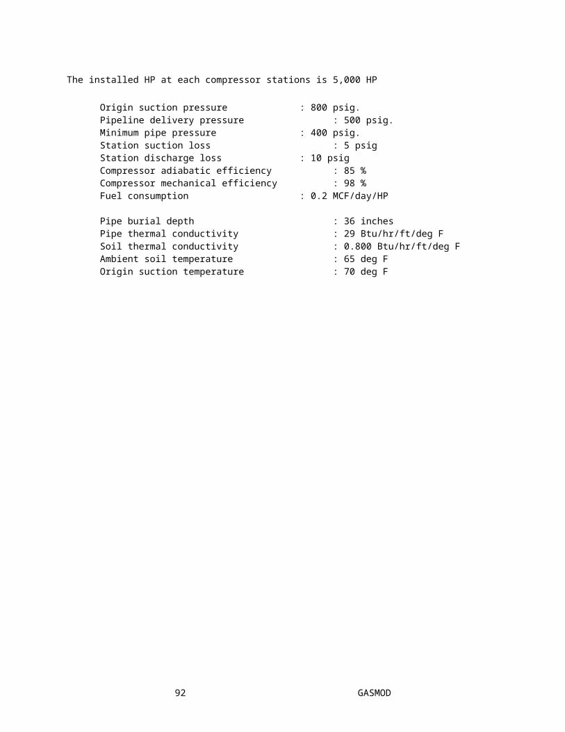
Total line pack in main pipeline = 6.4452 million std.cu.m

92 GASMOD