1: television signal transmission standards chapter 2
TRANSCRIPT

:11=1.110171.1-
Chapter 1: Television Signal Transmission Standards Chapter 2: Microwave Engineering for the Broadcaster Chapter 3: Satellite Earth Stations Chapter 4: Fiber Optic Video Transmission Systems Chapter 5: Aural Broadcast Studio Transmitter
and Intercity Relay Service

-

4.1
Television Signal Transmission Standards
INTRODUCTION
This chapter is intended to assist the broad- cast engineer in evaluating the quality of televi- sion program transmissions. It consists primari- ly of the text of NTC Report No. 7, with addi- tional material on audio signal measurements from EIA RS- 250 -B.
NTC Report No. 7 (1976) was prepared by the Network Transmission Committee of the Video Transmission Engineering Advisory Committee, a joint committee of television network broad- casters and the Bell System. It defines transmis- sion parameters, test signals, measuring methods, and performance objectives. The performance ob- jectives are applicable to an overall transmission system, including both local and inter -city relay facilities.
Since NTC -7 does not include audio channel standards, the audio section of the Electronic In- dustries Association Standards RS -250 -B (1976) has been included.
EIA RS -250 -B differs from NTC -7 primarily in that it includes performance objectives agreed upon by the television networks and AT &T for guaranteed performance for the coast to coast video networks. Since measuring methods and test signals are otherwise the same for the two stan- dards, the performance objectives may be com- pared, as on the following chart. In general, RS -250 -B is considered a more rigorous standard, reflecting industry -wide measures of performance, which may be used, for example, to test short, medium, satellite and long haul systems. NTC -7 is usually considered a standard for checking day-
to -day operation of a network television inter- connection system.
A third standard, said to be compatible with those EIA and NTC, is the AT &T Communica- tions "Commercial Television Transmission Spe- cification" (1984). As with RS- 250 -B, perfor- mance objectives are specified for short haul, medium haul, satellite, long haul, and end -to -end. AT &T also publishes similar standards for non- commercial television, premium grade audio and standard grade audio transmission.
A revised and updated version of EIA RS -250 has been in preparation and should be available some time in 1985.
Further information on acquiring complete copies of all three standards follows at the end of this chapter.
Using This Chapter The three -page chart presents a summary of
the tests and performance objectives of RS -250 -B and NTC -7. They are listed in the order consis- tent with RS- 250 -B, but there are references to the NTC -7 sections which follow. By referring to the chart and the complete test procedure, the reader may select the tests and performance objectives for a particular application.
For those familiar with NTC -7, the original order and numbering have been preserved.
To supplement NTC -7, the audio section of RS -250 -B has been included. These tests, Section 6, appear between NTC -7 Section 5 and the two Appendices.
4.1 -1

4.1 -2 Section 4: Program Transmission Facilities
TEST
NUMBER
VIDEO
PERFORMANCE TEST
TELEVISION PERFORMANCE STANDARDS FOR RELAY FACILITIES DISPLAYED
NTC -7 EIA RS 250 B VISUAL
SHORT HAUL MEDIUM HAUL SATELLITE LONG HAUL I
END
-TO-END EFFECT
AMPLITUDE
VS.
FREQUENCY
CHARACTERISTIC
WHITE FLAG
AMPUTUDE
ADJUSTED TO
1001RE UNITS
a) ALL FRE
QUENCY BURSTS
AMPLITUDES
SHALL BE:
SO5 IRE UNITS
hl COLOR BURST
AMPLITUDE
SHALL BE:
40 14 IRE UNITS
IRHBBBIBII THE MUST COMMON AND MOST OBVI- GUS LUMINANCE EFFECT RELATED TO LOW HIGH FREQUENCY RESPONSE IN THE VIDEO PASSBAND IS POOR RESOLU TION OR SOFTNESS OBSERVED IN THE DISPLAYED PICTURE. IT SHOULD ALSO BE NOTED THAT NONLINEAR PHASE CHARACTERISTICS ERISTICS CAN APPEAR AS A CONSEQUENCE OF THE FREQUENCY ROLL RESPONSE OF THE VIDEO PASS. BAND.
IN THE EVENT THAT THE VIDEO PASS - IS PEAKED AT THE UPPER LIMIT,
THIS WILL DISPLAY AN UNUSUAL CRISP. NESS OR ENHANCEMENT IN THE OIS. PLAYED PICTURE. THE USE OF HIGH FREQUENCY PEAKING CIRCUITS IN VIDEO EQUIPMENT, AND TRANSMISSION CHANNELS IS REFERRED TO AS "IMAGE ENHANCEMENT 'S
BIII E ¡;, I
"Eá "` "` ÌL
oW + "" l w
' - -
_ .or EYy
"' '- - - "ui - MMpI1IIII,`i1 YA LN
oz
0,
wiZ1.11ri:.%üa- = N
1 ii..uaaaaawaypp aaBE
Zg.:pFdB s NM oar
=_ "p¡: NTC 3.S iÌiiNi:! IBAND
r I I III "`°
e
NTC 3.6
CHROMINANCE TO
LUMINANCE
GAIN INEQUALITY
CHROMINANCE
AMPLITUDE
REFERENCED TO
UNE BAR SHALL
6E:
100 +3 IRE UNITS
1.ó,c1
+1 IRE UNITS -F4 IRE UNITS +4 IRE UNITS ±7 IRE UNITS ±7 IRE UNITS
THIS PROBLEM WILL AFFECT THE SATURATION LEVELS IN RECEIVED PIC.
UNDER SATURATED ATEACOLRS OVER OR
UNDER SATURATED COLORS.
THIS DISTORTION IS SOMETIME RE FERRED TO AS ''SATURATION ERRORS "'
NTC 3.7
CHROMINANCE
TO TO LUMINANCE
INEQUALITY
±75 RSEC ±20 RSEC ±33 RSEC +26 FISEC + 54 nSfC +60 nSfC
THIS DISTORTION IS MOST NOTICEABLE WITH RED LETTERING SMEARING INTO A NEUTRAL BACKGROUND. IN MORE SEVERE EXAMPLES OF THIS TION. THE EFFECT OF COLOR GHOST. LNG OR MISRE
RECEIVED IS DIS.
PLAYED ON THE RECEIVED PICTURE.
4 NTC 3.3
FIELD TIME
WAVEFORM
DISTORTION
<4 IRE UNITS
PEAK- TO-PEAK 3 IRE UNITS
PEAK -TO -PEAK
3 IRE UNITS
PEAK-TO-PEAK 3 IRE UNITS
PEAK-TO-PEAK 3 IRE UNITS
PEAK -TO PEAK
3IRE UNITS
PEAK -TO PEAK
OBVIOUS FIELD TIME ERRORS DIS. PLAY OBJECTIONAL VERTICAL SHAD -
MG RECEIVED
TOP TO BOTTOM IN THE RECEIVED PICTURE.
5 NTC 3.4
UNE TIME
DISTORTION
<4 IRE UNITS
PEAK -TO -PEAK
0.5 UNIT
PEAK-TO-PEAK 1 IRE UNIT
PEAK-TO-PEAK 1 IRE UNIT
PEAK-TO-PEAK 1.5 UNITS
PEAK-TO-PEAK 2 UNITS
PEAK -TO -PEAK
APPEARS AS SMEARING OR STREAKING FROM LEFT TO RIGHT IN RECEIVED PICTURE.
ALSO, UNEVEN SHADING MAY BE NO- TICED TILED FROM LEFT TO RIGHT. POOR CONTRAST NOTED.
6 NTC 3.5
SHORT TIME
WAVEFORM
DISTORTION
IT PULSE AMPS]. TODE SHALL BE:
100 +5 IRE UNITS
UNE-BAR EDGE
OVERSHOOT
SHALL NOT
EXCEED
10 IRE UNITS
IPEAK-TO -PEAK)
4 IRE UNITS
PEAK -TO -PEAK
4 IRE UNITS
PEAK -TO -PEAK
4 IRE UNITS
PEAK -TO -PEAK
6.5 IRE UNITS
PEAK- TO-PEAK
7 IRE UNITS
PEAK -TO -PEAK
THIS TYPE OF DISTORTION AFFECTS HORIZONTAL RESOLUTION :SOMETIMES REFERRED TO AS DEFINITION. ALSO, CONTOURING OR RINGING CAN BE OBSERVED WHEN
RESPONSE OF THEEVIDEO PASSBANO IS PRESENT.
NTC 3.12
LONG TIME
WAVEFORM
DISTORTION
(BOUNCE)
PEAK OVERSHOOT
AT BLANKING
SHALL NOT
EXCEED 5IRE
UNITS, SETTLING
TIME LESS
THAN 1 SEC
8 IRE UNITS
PEAK
3 SEC SETTLING
TIME
DIRE UNITS
PEAK
3 SEC SETTLING
TIME
B IRE UNITS
PEAK
3 SEC SETTLING
TIME
8 IRE UNITS
PEAK
3 SEC SETTLING
TIME
8 IRE UNITS
PEAK
3 SEC SETTLING
TIME
INTERMITTENT AND SLOW VARIATION IN PICTURE BRIGHTNESS.
THESE DISTORTIONS ARE USUALLY VIEWED OVER LONG PERIODS OF TIME. FLICKER IS AN EXAMPLE OF A LONG TIME DISTORTION.
8 NTC 3.2
INSERTION GAIN
VARIATION
SHALL NOT
EXCEED ZERO
+3 IRE UNITS
SHORT PERIOD
eq. 5 DEC.)
+1 IRE UNIT
MEDIUM PERIOD
(A9. 1 HR.)
+2 IRE UNITS
0.15 DB HOURLY
+0.1 OR OVER
ONE SEC
+0.3 DB HOURLY
+0.15 DB OVER
ONE SEC
01 DB HOURLY +0.15 DB OVER
ONE SEC
+0.45 OB HOURLY +0.25 08 OVER
ONE SEC
+0.5 DB HOURLY
+0.3 DB OVER
ONE SEC
MAY BE NOTED BY OVER OR UNDER CONTRASTED PICTURES IN MONO. CHROME TRANSMISSIONS ALSO, OVER OR UNDER CONTRASTED AND SAT URA7ED PICTURES IN COLOR TRgNS MISSIONS.
9 NTC 3.9
LUMINANCE
NON -LINEARITY
LARGEST DIP
FERENTIATED
PULSE REF AT
LOO IRE.
SMALLEST PULSE
NO LESS THAN
90 IRE UNITS
10% 50%
OIL 90 %APL
2% 4% 6% 8% 10%
NON LINEAR TRANSFER CHARAC TERISTICS IN A VIDEO CHANNEL WILL RESULT IN CONTRAST TTED
PICTURE U
TIVE TO THE TRANSMITTED PICTE IN SERIOUS PROBLEMS OCCUR COLOR SYSTEMS, SUCH AS HUE ANDSATURA. TION ERRORSRESULTING FROM NON UNIFORMITIES IN THE LUMINANCE
CHROMIINANCERINFORMATION. THE
NTSCM color television performance measurements for communication systems. (Page 1 of 3.)

Chapter 1: Television Signal Transmission Standards 4.1 -3
TEST
NUMBER
10 NTC 3.13
VIDEO PERFORMANCE
TEST
11 NTC 3.14
12 NTC 3.15
TELEVISION PERFORMANCE STANDARDS FOR RELAY FACILITIES
NTC-7 EIA RS-250-B
SHORT HAUL MEDIUM HAUL SATELLITE LONG HAUL END TO-END
DISPLAYED
VISUAL
EFFECT
DIFFERENTIAL Is%
GAIN I IS ME UNRSI 5% 4% 10%
THE VISUAL OBSERVATIONS NOTED AS A RESULT OF THIS DEGRADATION. ARE SATURATION ERRORS IN THE RECEIVED PICTURE INFORMATION.
DIFFERENTIAL
PHASE
CHROMINANCE TO
LUMINANCE
INT ER MO OULATION
13 NTC 3.10
CHROMINANCE
NON LINEAR GAIN
14 NTC 3.11
15 NTC 3.12
1.30 1.50 2.50 3.00
THE VISUAL OBSERVATIONS DIS PLAYED ON THE RECEIVED PICTURE ARE CHANGES OR ERRORS IN HUE AS
A FUNCTION OF LUMINANCE AMPLI TUDE VARIATIONS
3 IRE UNITS 1.0% 2.0%
SMALLEST SUR
CARRIER
AMPUTUOE
7R r211M: UNITS
LARGEST SUN.
CARRIER
AMPLITUDE
M !t ME UNITS
1.0%
2.0% 4.0% 4.0%
INCORRECT REPRODUCTION OF THE INCREASED SATURATED COLORED AREAS OF THE RECEIVED PICTURE
2.0% 2.0% 4.0% 5.0%
THE VISUAL EFFECT FOR THIS VIDEO IMPAIRMENT COULD ALSO BE THE IN-
CORRECT REPRODUCTION OF IN
CREASES SATURATED AREAS. HOW.
EVER, THIS MAY NOT BE APPARENT NY JUST OBSERVING THE RECEIVED PICTURE WITHOUT COMPARING IT TO
THE TRANSMITTED INFORMATION,
CHROMINANCE
NON- LINEAR PHASE
DYNAMIC GAIN
OF THE
PICTURE SIGNAL
<50 10 50
THE VISUAL OSSERVATION NOTES AT THE RECEIVER WOULD SE HUE
SHIFTING IN HIGHLY SATURATED AREAS.
DYNAMIC GAIN
AT 10% OR 90%
APL. REF 50%
API.
3 IRE UNITS
4%
16 NTC 3.12
17
18 NTC 3.16
19
DYNAMIC GAIN
OF THE
SYNCHRONIZING
SIGNAL
TRANSIENT
SYNCHRONIZING
SIGNAL
NON LINEARITY
DYNAMIC GAIN
AT 10% OR 90Y
APL. REF 5O%
APE
t1 IRE UNITS
3% 4%
SIGNAL TO -NOISE
RATIO
(10 KHZ 5.0 MHZ)
1%
>SI GS
ON MNi - 112 WIZ
7%
IF THE SYSTEM GAIN IS REDUCED AS
A FUNCTION Of APL, THE DYNAMIC RANGE OF THE VIDEO SIGNAL WILL
TYPICALLY BE COMPRESSED THIS
WILL CONTRIBUTE TO ALL NON-
LINEAR DISTORTIONSWITH REDUCED
CONTRAST RATIOS OIBPLAYED ON
THE RECEIVER PICTURE.
NONLINEAR TRANSFER CHARAC- TERISTIC OF THE VIDEO CHANNEL. THIS PROBLEM CONTRIBUTES TO
ALL NON-LINEAR DISTORTIONS AS A
FUNCTION Of APL.
SEE ABOVE DISCUSSION.
TYPICALLY A REDUCTION IN SYN CHRONIZING PULSE AMPLITUDE SE LOW A DEFINES THRESHOLD WILL RESULT IN LOSS OF PICTURE LOCK
HORIZONTAL, VERTICAL. OR 10TH.
4%
67 DB i 60 DB
SIGNAL TO -LOW
FREQUENCY NOISE
RATIO
10 10 KHZ)
53 DB
56 DB
5%
54DB 54DB
48 DB 50 DB 44 DB
SNOWEY PICTURE DISPLAYED ON
MONOCHROME MONITORS
ON COLOR MONITORS THE EFFECT
NOTED IS COLORED SNOW, ALSO
REFERRED TO AS "CONFETTI °.
43 DB
TYPICAL SOURCES of LOW ERE
DUENCY NOISE ARE POWER LINE OR
POWER SUPPLY RELATED.
OBSERVED VISUAL EFFECT FOR
POWER LINE OR SW MOSLEMS WOULD APPEAR AS ONE WIDE HORI ZONTAL AAR ACROSS THE SCREEN.
THE APPEARANCE OF TWO NARROW.
ER BARS INDICATES 111HZ RIPPLE
LEAKING IN FROM POWER SUPPLIES.
NTSC -M color television performance measurements for communication systems. (Page 2 of 3.)

4.1 -4 Section 4: Program Transmission Facilities
TEST
NUMBER
VIDEO PERFORMANCE
TEST
TELEVISION PERFORMANCE STANDARDS FOR RELAY FACILITIES DISPLAYED
NTC -7 EIA RS-250B
VISUAL
SHORT HAUL MEDIUM HAUL SATELLITE LONG HAUL END -TO-END EFFECT
20 / NTC
3.18
SIGNAL-TO-PERIODIC
NOISE RATIO
(300 HZ - 4.2 MHZ)
250 DB
1 KHZI
250 DB
It KHZ - 4.2 MHZ)
67 DB 62 DB 64 DB 58 DB 57 DB
OBSERVED VISUAL EFFECT OF EXTRANEOUS TONE IN THE DESIGNATED PASSIANO (ODON2
4.2 MHZ),
NOTES
WITH THE TUNE COUID BE FIVE OR MORE HORIZONTAL LINES NOTED ACROSS THE SCREEN OF VARY
INC INTENSITY THIS WOULD TYPICALLY OCCUR BELOW LINE FREQUENCY 1517/INHZ AT OR MULTIPLES OF LINE FREQUENCY. THE DISPLAYED VIDEO COULD INCLUDE FROM ONE WIDE VERTICAL COLUMN TO SEVERAL LINES URF.
NOTED HOWEVER
ACROSS THE SIGNALS
ARE SELDOM AT LINE FREQUENCY THERE. FORE
D. DIAGONAL LINES RACING WOULD BE
VIEWE
NTC 3.17
SIGNAL -TO- IMPULSE
NOISE RATIO
_> 23 D8
leg. IMPULSE
NOISE <1 IRE
PEAK -TD -PEAK,
FREQUENCY OF
OCCURENCES
1 PER MINUTE).
NOT SET NOT SET NOT SET NOT SET NOT SET
THE VISUAL EFFECT NOTED FOR IMPULSE NOISE DISPLAYED ON A MONOCHROME SYSTEM WOULD BE BLACK AND WHITE 0075 -RACING
ACROSS THE SCREEN IN A ZARO ANT. IN COLOR SYSTEMS'. BLACK AND WHITE, AND COLOR SPECKLES WOULD BE VIEWED.
22 NTC 3.19
SIGNAL -TO
CROSSTALK
NOISE RATIO ) 60 DB
THIS DISTORTION COULD TYPICALLY PRODUCE MANY DIFFERENT TYPES OF ERRATIC PATTERNS DISPLAYED
THE ON THE RECEIVED PICTURE. THE
OF NDOTHER DU
VIDEO SOURCES OR EXTRANEOUS TONES IN DISPLAYED PICTURE.
23 CONTINUITY OF
VIDEO SERVICE 99.99%
OBJECTIVE
99.99%
OBJECTIVE
99.99%
OBJECTIVE
99.99%
OBJECTIVE
99.99%
OBJECTIVE
24 K- FACTOR
K-FACTORS SPECIFICALLY RELATE TO THE MONOCHROME OR LUMI NANCE COMPONENT IN VIDEO SYS TEMS. THE PARTICULAR DISPLAYED VISUAL EFFECT WOULD BE OB. TAMED UNDER TEST NUMBER 5, (LINE TIME DISTORTION) AND TEST NUMBER 6, (SHORT TIME DISTOR.
SQUARE ASYMMETRY IN THE 2T SINE
RE PUISE DENOTE GROUP EN- VELOPE DELAY IN THE 1.3 MHZ REGION.
25 COLOR BURST
AMPLITUDE 40 IRE UNITS
±4 IRE UNITS
40 IRE UNITS
±0.5 IRE
BASED ON GAIN/ FREQUENCY
SPECIFICATION
40 IRE UNITS ±2.0 IRE
BASED ON GAIN/ FREQUENCY
SPECIRCATION
90 IRE UNITS ±20 IRE
BASED ON GAIN / FREQUENCY
SPECIFICATION
90 IRE UNITS ±3.0 IRE
BASED ON GAIN/ FREQUENCY
SPECIFICATION
40 IRE UNITS +3.0 IRE
BASED ON GAIN/ FREQUENCY
SPECIFICATION
LOW AMPLITUDE OF THE COLOR BURST WILL RESULT IN LOSS OF COLOR SNYCHRONINATION. LOSS OF
FIRST BE NOTICED NI WITH NA REDI
EFFECT ACROSS THE ENTIRE VIEW 1
DISPLAY. THIS IS SOMETIMES RE-
EFFECT). TFURTHERE REDUCTION 0OF THE REFERENCE BURST WILL TURN A COLOR TRANSMISSION INTO A
- MONOCHROME DISPLAY.
M.(' 5.1
RELATIVE BURST
GAIN ERROR
/0 IRE UNITS ±1 IRE UNIT
- - --
HIGH OR LOW COLOR SATURATION OBSERVED IN THE RECEIVED PIC- TURE ADJUSTED
AS A CONSEQUENCE MIR OU CONSEQUEN AMPLIFIER INSERTED IN THE SIGNAL CHANNEL. NOTE, THE EXISTENCE OR NON. EXISTENCE OF A PROCESSING AMPLI- FIER IN THE SIGNAL CHANNEL, MAY NOT BE APPARENT BY VISUAL OBSER NATION ALONE. - - - -- - -- --
27 NTC 5.2
RELATIVE BURST
PHASE ERROR ±10
A CHANGE OR VARIATION IN HUE OBSERVED IN THE RECEIVED PIC- ADJU ADJUSTED
CONSEQUENCE OFAMIS AMPLI-
FIER, INSE IN THE SIGNAL INSERTED VIDEO
IN THE
SIGNAL CHANNEL.
NOTE, THE EXISTENCE OR NON -
EXISTENCE OF A PROCESSING AMPII- FIER IN THE SIGNAL CHANNEL, MAY NOT BE APPARENT BY VISUAL OB- SERVATION ALONE.
Credit: Michael J. Shumila Member, Technical Staff RCA Laboratories David Sarnoff Research Center Princeton, NJ
NTSCM color television performance measurements for communication systems. (Page 3 of 3.)

Chapter 1: Television Signal Transmission Standards 4.1 -5
Section 3 *: Parameters, Measuring Techniques and Performance Objectives
GENERAL AND WAVEFORM TECHNOLOGY
This section describes the transmission para- meters, measuring techniques and performance objectives that are applicable to all video trans- mission facilities leased from the Bell System.
It should be noted that except where full -field test signals are essential to the measurement of a particular transmission parameter, e.g., field - time waveform distortion, the measuring tech- nique and its associated performance objective specified for each transmission parameter apply equally to both vertical interval test signals (VITS) and full -field test signals. Furthermore the per- formance objectives apply irrespective of the average picture level (APL) within the APL range 1007o to 90 %. This is an important point to re- member when making VITS measurements, par- ticularly during program transmission periods where control cannot be exercised over the APL value of picture signal. Many of the transmission parameters can be markedly affected by APL variations. Acordingly, the operator should allow sufficient time when making VITS measurements to ensure a good portion of the APL range is
explored by the picture signal before recording the test signal measurement. In every case the highest distortion measurement observed during this period should be recorded and then compared
'Section and test numbers are original NTC -7 numbers.
with the performance objective to determine whether or not the facility is within the stated objective.
Waveform measurement techniques described in this report are based on the IRE scale units of measurement (see Fig. 1) except where specif- ically noted otherwise. The waveform technology used throughout the report is in accordance with the definitions shown in Fig. 2 wherein the stan- dard composite color video signal is defined.
The two principal test signals that are required to conduct the various measurements described in this report are:
A. The composite test signal shown in Fig. 3, which consists of a line bar, a 2T pulse, a chrominance pulse, and a 5 -riser staircase signal.
B. The combination test signal shown in Fig. 4, which consists of a white flag, a multiburst and a 3 -level chrominance signal.
When conducting in- service VITS measurements the composite test signal shall be inserted on line 17, field 1, and the combination test signal shall be inserted on line 17, field 2.
NOTE: The performance objectives specified in this report pertaining to television transmission facilities, apply only when the recommend- ed test signals are originated directly at the designated broadcaster/ TELCO interface. No broadcaster maintained and operated equip- ment shall be used between the test signal generator output and the interface point.

4.1 -6
IRE unit s
120 -
100
80
60 -
40
20
0
-20
To
100
80 - 60 - 40 - 20
0-
20 - 40
.714 volt
.286 volt
Section 4: Program Transmission Facilities
Fig. 1. The IRE scale units. (For a 1V PP composite signal)
I VOLT
B
WAVEFORM TERMINOLOGY
A: The peak -to -peak amplitude of the composite color video signal
B: The difference between black level and blanking level (set- up)
C: The peak -to -peak amplitude of the color burst
L: Luminance signal -nominal value
M: Monochrome video signal peak - to -peak amplitude (M = L +S)
S: Synchronizing signal- ampli- tude
Tb: Duration of breezeway Ts1: Duration of line blanking period Ts y: Duration of line synchronizing
pulse Tu: Duration of active line period
Fig. 2. The standard composite color video signal.

Chapter 1: Television Signal Transmission Standards
IRE scale JMt!
'C:
6C
60
40
20
0
-20
40
12
4.1 -7
1 I 1
30 34 37 42 46 52 58 62
NOMINAL TIMING - MICROSECONDS
Fig. 3. The composite test signal.
IRE scale ,x,m
100 -
80 - 0 5 MHz
I
NH 2 3 358 4 2
MHz MHz MHz MHz
60 -
40 -
20 -
0
-20
40 I 1 T T 1
0 12 16 18 24 28 32 36 40 43 46 50 54 6062
NOMINAL TIMING - MICROSECONDS
Fig. 4. The combination test signal.

4.1 -8 _ Section 4: Program Transmission Facilities
3.2 INSERTION GAIN Definition: Insertion gain is defined as the difference, in
IRE units, between the peak -to -peak amplitude of a specified test signal at the receiving end of a television facility and the nominal amplitude of the test signal at the sending end.
Measurement: The line bar portion of the composite test signal
shown in Fig. 5 is used when measuring inser- tion gain. The test signal's amplitude must be ac- curately adjusted at the sending end prior to the commencement of the test. Similarly, the wave- form monitor at the receiving end should be prop- erly calibrated.
Following the above, the peak -to -peak ampli- tude of the test signal should be measured, in IRE units, at the receiving end using the points ap- proximating to b1 and b2 as shown in Fig. 5. The difference between the measured amplitude of the test signal and its nominal amplitude of 100 IRE units is the insertion gain of the televi- sion facility. If the measured amplitude is less than 100 IRE units then the insertion gain should be recorded with a negative sign. Such an exam- ple is shown in Fig. 6.
Performance Objectives: a. The insertion gain shall not exceed zero ± 3
IRE units. b. Variations in insertion gain shall not exceed
i. Short period (e.g., 5 seconds): ± 1 IRE unit.
ii. Medium period (e.g., 1 hour): ± 2 IRE units.
These variations in gain are permissible only with- in the range specified in objective a.
NOTE 1: The performance objectives shown above apply equally to full -field and in- service VITS measurements.
NOTE 2: Insertion gain may also vary as a function of APL. This is termed dynamic gain, and is covered in section 3.12.

Chapter 1: Television Signal Transmission Standards 4.1 -9
bi
I8us
Fig. 5. The line bar test signal.
Generator Output Specifications
b2
1. TIME OF RISE
Peak amplitude 100 ± 0.5 IRE units (reference white amplitude)
Line -time waveform less than 0.3 IRE units distortion
Time of rise and time of fall of bar edges (10 % -90 %)
t = 125 ± 5 nanoseconds with integrated sine - squared shape
Fig. 6. An example of negative insertion gain.
Insertion gain is
-3 IRE units.
IRE units -100
80
60
40
20
0
4.1 -10 Section 4: Program Transmission Facilities
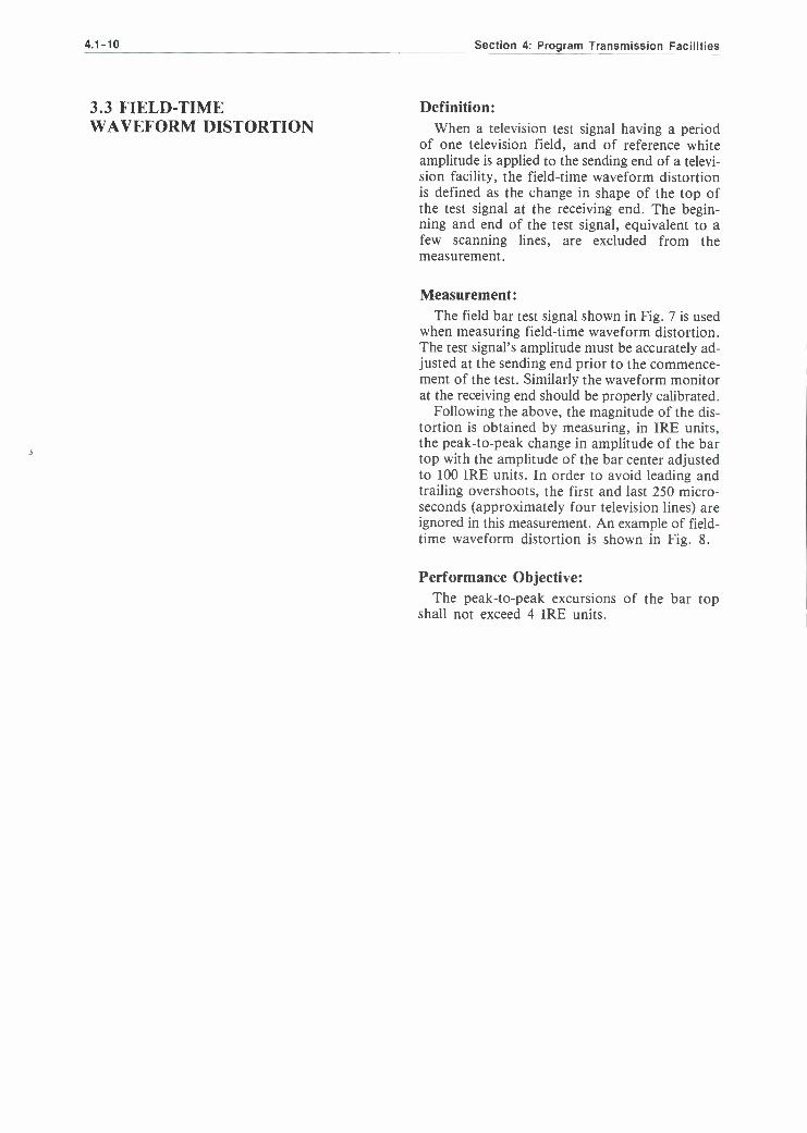
3.3 FIELD -TIME Definition: WAVEFORM DISTORTION When a television test signal having a period
of one television field, and of reference white amplitude is applied to the sending end of a televi- sion facility, the field -time waveform distortion is defined as the change in shape of the top of the test signal at the receiving end. The begin- ning and end of the test signal, equivalent to a few scanning lines, are excluded from the measurement.
Measurement: The field bar test signal shown in Fig. 7 is used
when measuring field -time waveform distortion. The test signal's amplitude must be accurately ad- justed at the sending end prior to the commence- ment of the test. Similarly the waveform monitor at the receiving end should be properly calibrated.
Following the above, the magnitude of the dis- tortion is obtained by measuring, in IRE units, the peak -to -peak change in amplitude of the bar top with the amplitude of the bar center adjusted to 100 IRE units. In order to avoid leading and trailing overshoots, the first and last 250 micro- seconds (approximately four television lines) are ignored in this measurement. An example of field - time waveform distortion is shown in Fig. 8.
Performance Objective: The peak -to -peak excursions of the bar top
shall not exceed 4 IRE units.

Chapter 1: Television Signal Transmission Standards 4.1 -11
8.33ms
Fig. 7. The field bar test signal.
Generator Output Specifications
Peak amplitude of 100 ± 0.5 IRE units luminance signal
Peak amplitude of synchronizing signal
40 ± 0.5 IRE units
Field -time waveform : less than 0.3 IRE units distortion
IRE units - 100
- 80
- 60
- 40
- 20
- - -20
-x'40
Horizontal component 100 IRE unit flat field of 52.45 microsecond nominal duration
NOTE: This signal should be generated with field and line synchronizing pulses.
Fig. 8. An example of fieidtime distortion.
Field -Time Distortion is 3 IRE units. ( +1, -2)

4.1 -12 Section 4: Program Transmission Facilities
3.4 LINE -TIME Definition: WAVEFORM DISTORTION When a television test signal having a period
of one television line and of reference white amplitude is applied to the sending end of a televi- sion facility, the line -time waveform distortion is defined as the change in shape of the top of the test signal at the receiving end. The begin- ning and end of the test signal, equivalent to a few picture elements, are excluded from the measurement.
Measurement: The line bar test portion of the composite test
signal shown in Fig. 9 is used when measuring line -time waveform distortion. The test signal's amplitude must be accurately adjusted at the sending end prior to the commencement of the test. Similarly the waveform monitor at the receiv- ing end should be properly calibrated.
Following the above, the magnitude of the dis- tortion is obtained by measuring, in IRE units, the peak -to -peak change in amplitude of the bar top with the amplitude of the bar center adjusted to 100 IRE units. The first and last one micro- second are ignored in this measurement. An ex- ample of line -time waveform distortion is shown in Fig. 10.
Performance Objective: The peak -to -peak excursions of the bar top
shall not exceed 4 IRE units.
NOTE: The performance objective shown above applies equally to both full -field and in- service VITS measurements.
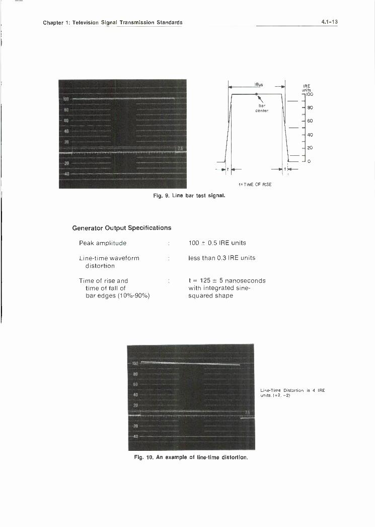
Chapter 1: Television Signal Transmission Standards 4.1 -13
Fig. 9. Line bar test signal.
IBus
bar center
D TIME OF RISE
Generator Output Specifications
Peak amplitude : 100 ± 0.5 IRE units
Line -time waveform : less than 0.3 IRE units distortion
Time of rise and time of fall of bar edges (10 % -90 %)
t = 125 ± 5 nanoseconds with integrated sine - squared shape
Fig. 10. An example of line-time distortion.
IRE units -'100
80
60
40
- 20
- 0
Line -Time Distortion is 4 IRE units. ( +2, -2)

4.1 -14 Section 4: Program Transmission Facilities
3.5 SHORT -TIME Definition: WAVEFORM DISTORTION If a short pulse or rapid step function of refer-
ence white amplitude and defined shape is ap- plied to the sending end of a television facility, the short -time waveform distortion is defined as the departure of the output pulse or step from its original shape. The choice of the half ampli- tude duration of the pulse or the rise -time of the step is determined by the nominal cutoff frequen- cy of the television facility.
Measurement: The line bar portion of the composite test signal
shown in Fig. 9 and the 2T pulse test signal shown in Fig. 11 are used when measuring short -time waveform distortion. The test signal's amplitude must be accurately adjusted at the sending end prior to the commencement of the test. Similarly the waveform monitor at the receiving end should be properly calibrated.
Following the above, the amplitude of the 2T pulse test signal is measured, in IRE units, hav- ing previously adjusted the amplitude of the line bar test signal to exactly 100 IRE units.
The peak -to -peak variations within the 1 micro- second intervals on either side (preceding and following) the T -step transitions (rise and fall) are then measured with the amplitude of the line bar test signal adjusted to 100 IRE units as measured between blanking and a point approximately 2 microseconds from the bar edge. (A graticule method of measuring short-time waveform distor- tion is currently under study by IEEE.) Examples of short -time waveform distortion are shown in Figs. 12 and 13.
Performance Objective: a. The 2T pulse amplitude shall be 100 ± 6
IRE units. b. The peak -to -peak amplitude variations pre-
ceding or following the T -step transitions to the line bar test signal shall not exceed 10 IRE units.
NOTE: The performance objectives shown above apply equally to both full -field and in- service vITS measurements.

Chapter 1: Television Signal Transmission Standards 4.1 -15
80
40
70
Fig. 11. The 2T pulse test signal.
Generator Output Specifications
Peak amplitude 100 ± 0.5 IRE units
Half amplitude 250 ± 10 nanoseconds duration (HAD)
2T Amplitude is 92 IRE units.
IRE units
-100
- 80
- 60
- 40
- 20
Amplitude variations following the T -step transition are 10 IRE units peak -to -peak.
Fig. 12. An example of short -time distortion as it affects the 2T pulse amplitude.
Fig. 13. An example of short-time distortion as it affects the edge response of the line bar.

4.1 -16 Section 4: Program Transmission Facilities
3.6 CHROMINANCE -LUMINANCE Definition: GAIN INEQUALITY When a test signal having defined luminance
and chrominance components is applied to the sending end of a television facility, the chromi- nance- luminance gain inequality is defined as the change in amplitude at the receiving end of the color component of the test signal relative to the luminance component.
Measurement: The chrominance pulse portion of the com-
posite test signal shown in Fig. 14 is used when measuring chrominance -luminance gain inequal- ity.* The test signal's amplitude must be accurate- ly adjusted at the sending end prior to the com- mencement of the test. Similarly the waveform monitor at the receiving end should be properly calibrated.
Following the above, the amplitude of the Chrominance Pulse Test Signal is measured in IRE units, having previously adjusted the ampli- tude of the line bar test signal to exactly 100 IRE units. This method is accurate to within 2% with up to 300 nanoseconds of chrominance -to -lumi- nance delay present. The convention of Fig. 17B shows how the chrominance pulse will look with different types of gain and delay distortion. If harmonic distortion is present on the chroma pulse, as evidenced by multiple irregularities of the baseline, this method is invalid and an ac- curate measurement cannot be made. Methods to make measurements in the presence of har- monic distortion are presently under study.
An example of low chrominance amplitude is shown in Fig. 15.
Performance Objective: The amplitude of the chrominance pulse shall
be 100 ± 3 IRE units.
NOTE: The performance objective shown above applies equally to both full -field and in- service VITS measurements.
This parameter is also called Realtive Chroma Level (RCL), and is expressed as a percentage of P -P chrominance referenced to the line bar amplitude, as shown in Fig. 15. Hence, the performance objec- tive expressed as RCL would be ± 6%.

Chapter 1: Television Signal Transmission Standards 4.1 -17
Fig. 14. The chrominance pulse test signal.
Generator Output Specifications
Peak amplitude
Half amplitude duration
Inherent chrominance luminance
a) gain inequality (RCL) b) delay inequality (RCT)
Subcarrier harmonic distortion
Irregularities in the pulse base line
100 ± 0.5 IRE units
t = 1562.5 ± 50 nanoseconds
less than ± 0.5 IRE (± 1 %) less than 5 nanoseconds, delayed or advanced
less than 1%
less than ± 0.5 IRE units
RE units -100
80
60
40
20
0
Chrominance Pulse Amplitude is 94 IRE units (RCL = - 12%) no delay inequality is present.
Fig. 15. An example of chrominanceIuminance gain inequality.

4.1-18 Section 4: Program Transmission Facilities
3.7 CHROMINANCE -LUMINANCE Definition: DELAY INEQUALITY When a test signal having defined luminance
and chrominance components is applied to the sending end of a television facility, the chrom- inance- luminance delay inequality is defined as the change in relative timing, at the receiving end, of the chrominance component of the test signal relative to the luminance component.
Measurement: The chrominance pulse portion of the corn -
posite test signal shown in Fig. 14 is used when measuring chrominance -luminance delay inequal- ity.* The test signal's amplitude must be acurately adjusted at the sending end prior to the com- mencement of the test. Similarly the waveform monitor at the receiving end should be properly calibrated.
Following the above, the amplitude of the chrominance pulse test signal should be adjusted to exactly 100 IRE units. The nomogram shown in Fig. 17A should be used to compute the magnitude of the chrominance -luminance delay inequality. If the chrominance component of the test signal starts with a positive going lobe then the chrominance -luminance delay inequality should be recorded as delayed chroma. The delay inequality can also be computed by the formula: CLDI (RCT) in ns = 20 fYl Y2. If harmonic distortion is present, as evidenced by multiple ir- regularities of the baseline, this method is invalid and an accurate measurement cannot be made. Methods to determine chrominance -luminance delay inequality in the presence of harmonic distortion are currently under study.
An example of chrominance -luminance delay inequality is shown in Fig. 16 below.
Performance Objective: The chrominance -luminance delay inequality
shall be no greater than 75 nanoseconds, ad- vanced or delayed chroma.
NOTE: The performance objective shown above applies equally to both full -field and in- service VITS measurements.
This parameter is also called Relative Chroma Time.

Chapter 1: Television Signal Transmission Standards 4.1-19
100 IRE
CLDI(RCT) is 240 Nanoseconds Delayed Chroma with no gain inequality present.
Fig. 16. An example of chrominance -luminance delay inequality.
PULSE AMPLITUDE NORMALIZED
Y2
DELAYED CHROMA ADVANCED CHROMA (WHEN YI IS (WHEN YI IS -)
t l' l'I'I Illll I' I'l'1 2 3 4 5 6 8 10 20 30 40 50
YI IRE unita
I I I I I} I II IIItIt+ I I I I I ( I I I I I CLDI (RCT)
20 30 40 5060 80 100 200 300 403 500 (nt)
Y2 IRE units
,1,11? 5° 10,410,T
NOMOGRAM COURTESY IEEE
Fig. 17A. Chrominance -luminance delay nomogram with measurement convention.
IRE _- (RCLin %.2o) units TOP OF LINE BAR AS REFE RENCE AMPLITUDE +o
100
o
_o
DELAYED(CHROMIA) ADVANC ED 1...---NO DELAY
LOW CHROMA (- RCL)
IF
Fig. 17B. Chrominance -luminance gain measurement convention.
1
41; 2
DELAYED(CH OMA) ADVANCED
HIGH CHROMA(+RCL)

4.1 -20 Section 4: Program Transmission Facilities
3.8 GAIN /FREQUENCY Definition: DISTORTION The gain /frequency distortion of a television
facility is defined as the variation in gain over the frequency band extending from the television field repetition frequency to the nominal cutoff frequency of the facility, relative to the gain at a suitable reference frequency.
Measurement: The multiburst portion of the combination test
signal shown in Fig. 18 is used when measuring gain /frequency distortion in the range from 500 kHz to 4.2 MHz. The test signal's amplitude must be accurately adjusted at the sending end prior to the commencement of the test. Similarly the waveform monitor at the receiving end should be properly calibrated.
Following the above, the amplitude of the white flag should be adjusted to exactly 100 IRE units and then the peak -to -peak amplitude of each burst frequency should be measured and record- ed. An example of gain /frequency distortion is shown in Fig. 19.
Performance Objective: With the white flag amplitude adjusted to 100
IRE units:
a. All frequency burst amplitudes shall be 50 + 3, -5 IRE units.
b. Color burst amplitude shall be 40 ± 4 IRE units.
NOTE: The performance objective shown above applies equally to both full -field and in- service VITS measurements.

Chapter 1: Television Signal Transmission Standards 4.1 -21
ill lit trttm1t
0.5 MHz MHz
RE unite
-100
75
2 3 MHz
3.58 4.2 50 MHz MHz MHz
25
I I I I I I 1 1 1
0 4 6 12 16 20 24 28 31
microseconds
Fig. 18. The multiburst test signal.
Generator Output Specifications
A) White Flag
Peak amplitude
Time of rise and time of fall of flag edges
Overshoot
Tilt
B) Multiburst Frequencies
All half -amplitude points of all burst frequencies
100 ± 1 IRE unit.
derived from the shaping network of the 2T sine - squared pulse.
less than ± 1 IRE unit.
less than ± 1 IRE unit.
50 ± 1 IRE unit.
(The starting point of each burst frequency shall be at zero phase of each sinewave.)
Peak -to -peak amplitude of all bursts 50 ± 0.5 IRE units.
d0
(4 ,Wiliïfl ll1 ár.
Fig. 19. An example of gain /frequency distortion.
-0
In this example, high frequency roll -off is shown. The burst am- plitudes vary from 50 IRE units in the 500 kHz burst to 42 IRE units in the 4.2 MHz burst.

4.1-22 Section 4: Program Transmission Facilities
3.9 LUMINANCE NON -LINEAR Definition: DISTORTION For a particular value of average picture level
(APL), the non -linear distortion of the luminance signal is defined as the departure from propor- tionality between the amplitude of a small unit step function at the sending end of a television facility and the corresponding amplitude at the receiving end, as the level of the step is shifted from blanking level to white level.
Measurement: The modulated 5 -riser staircase portion of the
composite test signal shown in Fig. 20 is used when measuring luminance non -linear distortion. The test signals amplitude at each step level must be accurately adjusted at the sending end prior to the commencement of the test. Similarly the waveform monitor at the receiving end should be properly calibrated.
Following the above, the test signal is passed through a differentiating and shaping network of the type shown in Fig. 21 with the output of the network connected to the waveform monitor being used for the measurement. The function of the network is that of transforming the test signal into a train of 5 pulses of equal amplitude under zero distortion conditions. The gain of the waveform monitor should be increased to the point where the largest pulse amplitude is 100 IRE units and then the amplitude of the smallest pulse can be measured and recorded. This is the Lumi- nance non -Linear Distortion at 50% APL. The above measurement procedure should be repeated using the same test signal transmitted on every fifth television line with intermediate lines set at blanking level for a 10% APL value and then at peak white for a 90% APL value.*
An example of Luminance non -Linear Distor- tion is shown in Fig. 22.
Performance Objective: With the largest pulse amplitude adjusted to
100 IRE units, the difference between it and the smallest pulse amplitude shall not be greater than 10 IRE units at 10 %, 50 %, or 90% APL.
NOTE: The performance objectives above also apply to in- service VITS measurements.
*For in- service VITS measurements the procedures outlined in Sec- tion 3 introduction should be followed.

Chapter 1: Television Signal Transmission Standards 4.1 -23
IRE unit
120 - 100
BO
60
40
20
0
-20
4 7 10 13 16 19 20 miaoNCmrtt
Fig. 20. The modulated 5 -riser staircase test signal (see section 3.13 for chrominance specifications).
Generator Output Specifications Peak amplitude of
each riser
Rise time of each riser
Step duration
Tilt on any step
Overshoot on any step
24.56
6265 11.19
601.1 KHz
1551.8 KHz
428.3 INPUT OUTPUT
n
8305 1471 35.23 t980
601.1 KHz
Inductances on given F uH, ccpacitomes in pF.
Fig. 21. Differentiating and shaping network for luminance non -linearity measurement.
shall be such that the luminance non -linear distortion shall be greater than 99.5 IRE units.
250 ± 10 nanoseconds
3.0 ± 0.1 usecs; final step 4.0 ± 0.1 microseconds (4.0 ± 0.1 microseconds at blanking level).
less than 0.3 IRE units
less than 0.3 IRE units
Luminance Non -Linear Distortion is 4 IRE units.
Fig. 22. An example of luminance non-linear distortion.

4.1 -24 Section 4: Program Transmission Facilities
3.10 CHROMINANCE NON -LINEAR Definition: GAIN DISTORTION
For fixed values of luminance level and average picture level, the non -linear gain distortion of the chrominance signal is defined as the departure from proportionality between the amplitude of the chrominance subcarrier at the sending end of a television facility and the corresponding ampli- tude at the receiving end as the amplitude of the subcarrier is varied from a specified minimum value to a specified maximum value.
Measurement: The 3 -level chrominance portion of the com-
bination test signal shown in Fig. 23 is used when measuring chrominance non -linear gain distor- tion. The test signal's amplitude at each chrominance level must be accurately adjusted at the sending end prior to the commencement of the test. Similarly the waveform monitor at the receiving end should be properly calibrated.
Following the above, the test signal is passed through a high -pass filter network* and the out- put of the network is connected to the waveform monitor being used for the measurement. The gain of the waveform monitor is adjusted to the point where the middle subcarrier amplitude is exactly 40 IRE units and then the amplitude of the largest and smallest subcarrier levels are measured and recorded. An example of chromi- nance non -linear gain distortion is shown in Fig. 24.
Performance Objective: With the middle subcarrier amplitude adjusted
to 40 IRE units the amplitude of the other two subcarrier levels shall be:
a . The smallest subcarrier amplitude shall be 20 ± 2 IRE units.
b. The largest subcarrier amplitude shall be 80 ± 8 IRE units.
NOTE: The performance objective shown above applies equally to both full -field and in- service VITS measurements.
*The chroma filter network incorporated into most television wave- form monitors is suitable for this test.

Chapter 1: Television Signal Transmission Standards 4.1 -25
00
lU
10
40 -
IRE
unit 100 - 90
80
70
60
50
40
30
20
10
0-
4 8 microseconds
Fig. 23. The 3-level chrominance test signal.
Generator Output Specifications
Peak -to -peak ampli- tudes of the 3- levels
Sub -carrier fre- quency phase
Rise and fall of chrominance envelopes
Duration of entire signal
20,40 and 80 IRE units 0.5 IRE units
14
90° ± 1° relative to reference burst; 0° ± 0.2° any one
relative to the other two.
400 ± 25 nanoseconds
14 ± 0.5 microseconds
The chrominance non -linear gain distortion is evidenced by the largest burst being equal to 64 IRE units.
Fig. 24. An example of chrominance non-linear gain distortion.

4.1 -26 Section 4: Program Transmission Facilities
3.11 CHROMINANCE Definition: NON -LINEAR For fixed values of luminance signal level and PHASE DISTORTION average picture level, the non -linear phase distor-
tion of the chrominance signal is defined as the variation in phase of the chrominance subcarrier at the receiving end of a television facility as the amplitude of the subcarrier is varied from a specified minimum value to a specified maximum value.
Measurement: The 3 -level chrominance portion of the com-
bination test signal shown in Fig. 23 is used when measuring chrominance non -linear phase distor- tion. The test signal's amplitude and phase at each chrominance level must be accurately adusted at the sending end prior to the commencement of the test. Similarly the waveform monitor and phase comparator (e.g., vectorscope) at the receiv- ing end should be properly calibrated.
Following the above, the test signal should be fed through a high pass filter network to the phase comparator (or directly to the vectorscope). Under zero distortion conditions the phase at each level of the 3 -level chrominance test signal should be - 90 ° relative to the phase of the color burst (see Fig. 25).
The phase of the three levels of the test signal should be measured relative to the phase of the color burst and recorded.
The peak -to -peak variation of the phase of the 3 -level chrominance test signal is the difference between the largest and smallest readings obtained.
It should be noted that processing amplifiers can change the phase of the test signal chromi- nance information relative to the phase of the col- or burst. Care should be taken to ensure a pro- cessing amplifier is not in the circuit during tests of this kind on television facilities.
An example of chrominance non -linear phase distortion is shown in Fig. 26.
Performance Objective: The peak -to -peak phase variation of the 3 -level
chrominance test signal shall not exceed 5 °.
NOTE: The performance objective shown above applies equally to both full -field and in- service VITS measurements.

Chapter 1: Television Signal Transmission Standards 4.1 -27
0°
Fig. 25. Chrominance non -linear phase distortion display showing zero distortion.
The chrominance non -linear phase distortion is 6 °.
Fig. 26. An example of chrominance non -linear phase distortion.
4.1 -28 Section 4: Program Transmission Facilities
3.12 DYNAMIC GAIN Definitions: DISTORTIONS If, at the sending end of a television facility,
the average picture level (APL) of a video signal is stepped from a low value to a high value, or vice versa, the operating point within the transfer characteristic of the system may be affected and introduce various distortions on the receiving end. This section covers two such distortions known, respectively, as long -time waveform distortion and dynamic gain.
Long -Time Waveform Distortion (Bounce)*
Measurement: The flat -field `bounce' test signal, as shown in
Fig. 27, is used when measuring long -time wave- form distortion. The test signal is switched be- tween 10 and 90 IRE units, at an appropriate rate, while the following measurements are made on a properly calibrated dc- coupled oscilloscope or waveform monitor, with any internal clamp in the instrument disabled.
With the waveform monitor on the field rate, observe any instantaneous peak excursion of the blanking level when the switch from 10 to 90 IRE, or vice versa, is made and record in IRE units. Also, observe the time necessary for blanking to settle to within 1 IRE unit of its final position. This may be as long as several seconds and the blanking level may undergo several peak -to -peak changes before stabilizing.
If an oscilloscope is used, a sweep time of 1
sec. /cm will generally enable the entire transient to be observed. The Tektronix 1480 MOD. 6 or 7 is presently the only waveform monitor with a slow sweep feature.
A photograph of this slow sweep is the best method of observing these distortions.
An example of long -time waveform distortion is shown in Fig. 28.
Performance Objectives: Peak overshoot at blanking shall be no greater
than 5 IRE units and the time for blanking to settle to within 1 IRE unit of its final level shall be less than 1 sec.
NOTE: This distortion only occurs when the APL change is accom- panied by a change in dc component.
*For in- service measurement of long -time waveform distortion the pro- cedure outlined in Section 3 introduction should be followed.

Chapter 1: Television Signal Transmission Standards
40 .,_
IRE units
100 - 90 80
60
40
20
o
-20
-40 52.45 us
Fig. 27. The flat-field bounce test signal (90% APL value shown).
Generator Output Specifications
Time of rise and fall of bar edge
Bar Duration Bar Amplitude
Tilt
Time of Transition (10 -90 or 90 -10)
Rate of Transition
Peak overshoot is 50mV (7 IRE), settling time .75 sec. sweep = 1 sec. /CM gain = .2V /CM (DC- Coupled)
derived from the shaping network of the sine -squared pulse. nominally 52.45 microseconds (High) 90 ± 1 IRE unit (Low) 10 ± .5 IRE units
Less than 1 IRE unit (10 -90 IRE units)
Less than 10 microseconds
5 sec.
Fig. 28. An example of long-time waveform distortion.
4.1 -29

4.1 -30 Section 4: Program Transmission Facilities
Dynamic Gain* Measurement: Switch the flat -field test signal out of the
`bounce' mode and select 50% APL (Fig. 29A). Next, switch the waveform monitor to display the composite test signal on line 17, field one (Fig. 3). If necessary, normalize the gain of the wave- form monitor for 100 IRE units at bar center. This is the reference amplitude for the following measurements.
Next, switch the test signal to 10% APL and observe and record, in IRE units, any change in amplitude of the line bar and /or synchronizing pulses. Finally, select 90% APL and record again any change in amplitude of the line bar and /or synchronizing pulses from the reference amplitude at 50% APL.
Examples of dynamic gain distortion are shown in Fig. 29B and C.
Performance Objectives: At 10% or 90% APL, dynamic gain -picture
shall not exceed ± 3 IRE units and dynamic gain - sync shall not exceed ± 2 IRE units referenced to the amplitude at 50% APL.
NOTE: This distortion may occur with or without a change in dc com- ponent accompanying the APL change.
For in- service measurements of dynamic gain the procedure outlined in Section 3 introduction should be followed.

Chapter 1: Television Signal Transmission Standards 4.1 -31
Full field test signal at 50% APL Fig. 29A.
Full field test signal at 10`,. APL
Line 17 field one, reference amplitude Picture 100 IRE units
Sync 38 IRE units
80
20 -
20
Fig. 29B. Dynamic gain distortion at 10% APL is
Picture: -3 IRE units Sync: +2 IRE units
Full field test signal at 90% APL Fig. 29C.
Dynamic gain distortion at 90% APL is Picture: +3 IRE units
Sync: 0 IRE units

4.1 -32 Section 4: Program Transmission Facilities
3.13 DIFFERENTIAL GAIN Definition: If a small constant amplitude of chrominance
subcarrier, superimposed on a luminance signal, is applied to the sending end of a television facili- ty, the differential gain is defined as the change in amplitude of the subcarier at the receiving end as the luminance varies from blanking level to white level, the average picture level being main- tained at a particular value.
Measurement: The modulated 5 -riser staircase portion of the
composite test signal shown in Fig. 30 is used when measuring differential gain. The test signal's amplitude at each step level must be accurately adjusted at the sending end prior to the corn- mencement of the test. Similarly the waveform monitor at the receiving end should be properly calibrated.
Following the above, the test signal should be fed through a high -pass filter network* and the output of the network connected to the waveform monitor being used for the measurement. The gain of the waveform monitor is then adjusted until the highest subcarrier peak -to -peak ampli- tude is exactly 100 IRE units. The peak -to -peak amplitude of the lowest subcarrier is then mea- sured. The difference between the highest sub - carrier amplitude and the lowest subcarrier amplitude is the differential gain distortion at 50% APL. The above measurement procedure should be repeated using the same test signal transmitted on every fifth television line with in- termedite lines set at blanking level for a 10% APL value and then at peak white level for a 90% APL value. The maximum differential gain dis- tortion measured should be recorded. **
An example of differential gain distortion is shown in Fig. 31.
Performance Objective: At 10 %, 50 %, and 90% APL, the differential
gain shall not exceed 15 percent (15 IRE units).
NOTE: The performance objective shown above also applies to the in- service VITS measurement.
The chroma filter network incorporated into most television waveform monitors is suitable for this test.
"For in- service VITS measurement of differential gain the procedure outlined in Section 3 introduction should be followed.

Chapter 1: Television Signal Transmission Standards 4.1 -33
IRE sent.
120-
100 -
80 -
60 -
40
20
0-
-20 -
Fig. 30. The modulated 5-riser staircase test signal.
I 1
4 7 10 13 16 19 20 microseconds
Generator Output Specifications
(In addition to the luminance specifications shown with Figure 20 in Section 3.9)
Chrominance ampli- 40 ± 0.5 IRE units tude
Inherent differential gain
and differential phase
Rise and fall times of the modulation envelope
Phase of chromi- nance signal rel- ative to reference burst phase
less than 0.5 percent
less than 0.2°
400 ± 25 nanoseconds
0° ± 1.0° over the range 10% to 90% APL
Fig. 31. An example of differential gain distortion.
Differential gain is 16 percent.

4.1 -34 Section 4: Program Transmission Facilities
3.14 DIFFERENTIAL PHASE Definition: If a constant amplitude of chrominance sub -
carrier without phase modulation, superimposed on a luminance signal, is applied to the sending end of a television facility, the differential phase is defined as the change in the phase of the sub - carrier at the receiving end as the luminance varies from blanking level to white level, the average picture level being maintained at a particular value.
Measurement: The modulated 5 -riser staircase portion of the
composite test signal shown in Fig. 30 is used when measuring differential phase. The test signal's amplitude and its subcarrier phase at each step level must be accurately adjusted at the send- ing end prior to the commencement of the test. Similarly the waveform monitor and phase corn - parator (e.g., vectorscope) at the receiving end should be properly calibrated. A vectorscope dis- play of differential phase with zero distortion is shown in Fig. 32.
Following the above, the test signal should be fed through a high -pass filter network to the phase comparator (or directly to the vectorscope). The differential phase distortion is the measured peak -to -peak change in subcarrier phase at 50% APL. The above measurement procedure should be repeated using the same test signal transmit- ted on every fifth television line with intermediate lines set at blanking level for a 10% APL value and then at peak white level for a 90% APL value. The maximum differential phase distortion should be recorded.*
An example of differential phase distortion is shown in Fig. 33.
Performance Objective: At 10 07o, 50% and 90% APL the differential
phase shall not exceed 5 degrees.
NOTE: The performance objective shown above also applies to the in- service VITS measurement.
For in- service VITS measurement of differential phase the procedure outlined in Section 3 introduction should be followed.

Chapter 1: Television Signal Transmission Standards 4.1 -35
Fig. 32. Vectorscope display of differential phase showing zero distortion (between arrows).
Fig. 33. Vectorscope display showing differential phase distortion (between arrows).

4.1 -36 Section 4: Program Transmission Facilities
3.15 CHROMINANCE -TO- Definition: LUMINANCE INTERMODULATION If a luminance signal of constant amplitude is
applied to the sending end of a television facili- ty, the intermodulation is defined as the varia- tion of the amplitude of the luminance signal at the receiving end resulting from the superimposi- tion on the luminance signal of a chrominance signal of specified amplitude.
Measurement: The 3 -level chrominance portion of the com-
bination test signal shown in Fig. 34 is used when measuring chrominance -to- luminance distortion. The test signal's amplitude at each chrominance level must be accurately adjusted at the sending end prior to the commencement of the test. Similarly the waveform monitor at the receiving end should be properly calibrated. A waveform monitor display of chrominance -to- luminance in- termodulation with zero distortion is shown in Fig. 35.
Following the above, the test signal is passed through a low -pass filter network* the output of which is connected to the waveform monitor being used for the measurement. The chromi- nance-to- luminance intermodulation is the max- imum amplitude departure in IRE units of the filtered luminance pedestal from the amplitude of that portion of the luminance pedestal which did not contain the superimposed subcarrier, with the pedestal adjusted to exactly 50 IRE units.
An example of chrominance -to- luminance in- termodulation is shown in Fig. 36.
Performance Objective: Chrominance -to- luminance intermodulation
shall displace the luminance component no more than 3 IRE units from the 50 IRE unit reference level.
NOTE: The performance objective shown above applies equally to both full -field and in- service VITS measurements.
*The low -pass filter network incorporated into most television waveform monitors is suitable for this test.

Chapter 1: Television Signal Transmission Standards 4.1 -37
RE unit.
100- 90
80 -
70
60 - 50
40 - 30
20 - 10
o
Fig. 34. The 3-level chrominance signal.
Generator Output Specifications
Peak -to -peak ampli- tudes of the 3- levels
Sub -carrier fre- quency phase
Rise and fall of chrominance envelopes
Duration of entire signal
2ä;
40
Fig. 35. Waveform monitor display showing zero chrominanceluminance intermodulation.
8 14
mcroeaconaa
20,40 and 80 IRE units 0.5 IRE units
90 °±- 1° relative to reference burst; 0° ± 0.2° any one relative to the other two.
400 ± 25 nanoseconds
14 ± 0.5 microseconds
The chrominance -to- luminance intermodulation is + 3 IRE units.
Fig. 36. Waveform monitor display showing chrominance luminance
intermodulation distortion.

4.1 -38 Section 4: Program Transmission Facilities
3.16 RANDOM NOISE -WEIGHTED Definition: The signal -to- weighted noise ratio of a televi-
sion facility is defined as the ratio, expressed in decibels, of the nominal amplitude of the lumi- nance signal (100 IRE units) to the RMS ampli- tude of the noise measured at the receiving end after band -limiting and weighting with a specified network. The measurement should be made with an instrument having, in terms of power, a time constant or integrating time of 0.4 seconds.
Measurements: In general, the random noise -weighted mea-
surement should be made with an RMS reading instrument with the video signal removed from the television facility and the input to the facility terminated in its characteristic impedance. However, the measurement can also be made either with a flat -field test signal as shown in Fig. 37 or using a specified line in the vertical blank- ing interval which is kept free of picture infor- mation, provided the measuring instrument ac- curately integrates the measured noise over the full -field period. In all of the above measurements the band -limiting and weighting networks shown in Fig. 38 shall be inserted at the receiving end of the television facility prior to the noise measur- ing instrument.
The signal -to- weighted noise ratio in decibles can be computed using the following formula:
Signal -to- weighted noise (dB) =
20 loglo P -P signal amplitude RMS weighted noise
An example of random noise is shown in Fig. 39.
Performance Objective: The signal -to- random noise ratio shall be
greater than or equal to 53 dB.
NOTE: Appendix II describes a technique for approximating weighted video random noie.

Chapter 1: Television Signal Transmission Standards 4.1 -39
80
40 _
40
IRE unts
100
80
Fig. 37. The 100% flat field test signal.
Generator Output Specifications
Time of rise and fall
52.45 us
derived from the shaping network of the sine - squared pulse.
Amplitude : 100 ± 1 IRE unit.
Tilt : less than 1 IRE unit.
Time of bar duration nominally 52.45 microseconds.
VIDEO
FACILITY
SEE FIG. 38A SEE FIG. 38B SEE FIG. 38C
4.2 MHz LPF 10 KHz HPF WEIGHTING
NETWORK
Fig. 38 Band limi ing and weighting network for measurement of random noise -weighted.
Fig. 39. An example of random noise.
75 RMS OHMS

4.1 -40 Section 4: Program Transmission Facilities
o
75n
3.42
7.903 MHz
tt
118
11-13-41
1.82 2.04 1YY71_ YYYL
4.625 10-9-0 MHz
646
T509 T 670 T 551
5.162 MHz
464
4*-41,--43
75n
309
o Inductances are given in uH, and capacitances in pF. Q
measured at 5 MHz is between 80 and 125 for all inductors.
Fig. 38A. Low -pass filter for use in noise measurements (lc = 4.2 MHz).
.139 .196
INPUT 0757 3.12 OUTPUT
75n 75n r
0 4 o Inductances are given in MH, capacitances in pF. Q measured at
10 kHz should be 100 or more.
Fig. 38B. High -pass Filter (fc = 10 kHz).
23.esn
Capacitances are Oven in pF, inductances in W. Capacitor and resistor tolerance 1%.
Insertion loss (d8) = IO[I(f /f,)2][I(f /f2 lop,o
[1 *(f/13)21 where f, = 0.270MHz, f2 =1.37MHz,and f3= 0.390 MHz.
Fig. 38C. Random noise weighting network.

Chapter 1: Television Signal Transmission Standards 4.1 -41
3.17 IMPULSIVE NOISE
Definition: The signal -to- impulsive noise ratio of a televi-
sion facility is defined as the ratio, expressed in decibels, of the nominal amplitude of the lumi- nance signal (100 IRE units) to the peak -to -peak amplitude of the noise.
Measurement: The flat -field test signal shown in Fig. 37 is
used when measuring impulsive noise. The test signal's amplitude must be accurately adjusted to 100 IRE units at the sending end prior to the com- mencement of the test. Similarly the waveform monitor at the receiving end should be properly calibrated.
Following the above, the test signal's amplitude should be adjusted to be exactly 100 IRE units at the receiving end and the waveform display then examined closely to determine if impulsive noise interference (occasional random spikes or transients) is present. The peak -to -peak amplitude of the interference is then measured, in IRE units,
and recorded. To compute the signal -to- impulsive noise ratio in decibels, the following formula can be used:
Signal -to- impulsive noise (dB) =
20 logro peak -to -peak amplitude
of impulsive noise
100 IRE units
Alternatively, the actual peak -to -peak amplitude of the impulsive noise, in IRE units, can be used directly to determine if the television facility meets the performance objective stated below.
An example of impulsive noise interference is shown in Fig. 40.
Performance Objective: The impulsive noise shall be no greater than
7 IRE units peak -to -peak which equals a signal - to- impulsive noise ratio of no greater than 23 dB. The frequency of occurrence of noise impulses shall not exceed one per minute.
Fig. 40. An example of impulsive noise interference.
Impulsive noise is 12 IRE units peak -to -peak.

4.1 -42 Section 4: Program Transmission Facilities
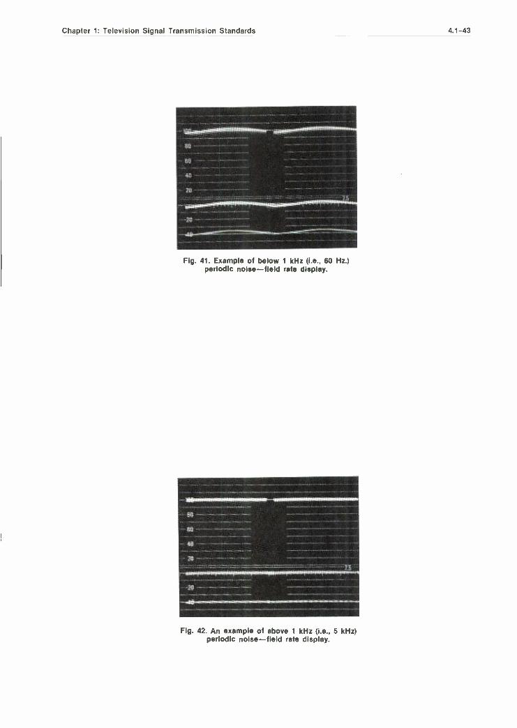
3.18 PERIODIC NOISE Definition: The signal -to- periodic noise ratio is defined as
the ratio in decibels of the nominal amplitude of the luminance signal (100 IRE units) to the peak - to -peak amplitude of the noise. Different per- formance objectives are sometimes specified for periodic noise (single frequency) between 1 kHz and the upper limit of the video frequency band and for power supply hum, including low -order harmonics.
Measurement: The flat -field test signal shown in Fig. 37 is
used when measuring periodic noise. The test signal's amplitude must be accurately adjusted to 100 IRE units at the sending end prior to the com- mencement of the test. Similarly the waveform monitor at the receiving end should be properly calibrated.
Following the above, the test signal's amplitude should be adjusted to be exactly 100 IRE units at the receiving end and the waveform display then examined to determine if periodic noise in- terference is present. The peak -to -peak amplitude, in IRE units, of periodic noise which is low - frequency in nature (power -supply hum, etc.) should be measured and recorded separately from the periodic noise in the nominal frequency range 1 kHz to 4.2. MHz.* Examples of periodic noise interference are shown in Figs. 41 and 42. To compute the signal -to- periodic noise ratio in decibels the following formula can be used:
Signal -to- periodic noise (dB) =
20 logro peak -to -peak amplitude
of periodic noise
100 IRE units
Performance Objective: The signal -to- periodic noise ratio, a. below 1 kHz (including power -supply hum
and lower order harmonics) shall be greater than or equal to 50 dB.
b. between 1 kHz and 4.2 MHz ** shall h greater than or equal to 50 dB.
NOTE: In specific instances where an exact measurement must be made, a spectrum analyzer or a frequency -selective voltmeter should be used. As these devices are normally RMS reading instruments, 9 dB should be substracted from the performance objective (to convert from peak -to -peak noise to RMS noise).
9t may be necessary to use the high -gain setting on the waveform monitor when making this measurement. If so, care should be taken to ensure that it is properly calibrated.
The low -pass filter network shown in Figure 38A should be used when measuring periodic noise interference in the range 1 kHz to 4.2 MHz.
Chapter 1: Television Signal Transmission Standards 4.1 -43
Fig. 41. Example of below 1 kHz (i.e., 60 Hz.) periodic noise -field rate display.
Fig. 42. An example of above 1 kHz (i.e., 5 kHz) periodic noise -field rate display.

4.1 -44 Section 4: Program Transmission Facilities
3.19 CROSSTALK NOISE Definition: The signal -to- crosstalk ratio is defined as the
ratio, in decibels, of the nominal amplitude of the luminance signal (100 IRE units) to the peak - to -peak amplitude of the interfering waveform.
Measurement: The flat -field test signal shown in Fig. 37 is
used when measuring crosstalk. The test signal's amplitude must be accurately adjusted to 100 IRE units at the sending end prior to the commence- ment of the test. Similarly the waveform monitor at the receiving end should be properly calibrated.
Following the above, the test signal's amplitude should be adjusted to be exactly 100 IRE units at the receiving end. The waveform display and a suitable broadcast -quality picture monitor can then be examined to determine if crosstalk in- terference is present. The peak -to -peak amplitude of the interfering waveform is then measured, in IRE units, and recorded.*
To compute the signal -to- crosstalk ratio in decibles the following formula can be used:
Signal -to- crosstalk (dB) =
20 logro peak -to -peak amplitude
of crosstalk
100 IRE units
Performance Objective: The signal -to- crosstalk ratio shall be greater
than or equal to 60 dB. **
*It may be necessary to use the high gain setting on the waveform monitor when making this measurement. If so, care should be taken to ensure that it is properly calibrated.
* *The low -pass filter network shown in Figure 38A should be used when measuring crosstalk noise interference.

Chapter 1: Television Signal Transmission Standards 4.1 -45
Section 4: Interconnection Requirements
INTRODUCTION This section defines the accepted standard in-
terconnection requirements that both the Bell System and the major television networks must comply with at their common interface points. Deviations from these requirements are permit- ted only if mutually agreed upon prior to the pro- vision and acceptance of the service.
IMPEDANCE At the points of interconnection between the
customer and the telephone company, the input and output impedance (Z4), of each link shall be specified as unbalanced to ground.
Performance Objective: Nominally 75 ohms resistive, unbalanced to
ground.
SIGNAL AMPLITUDE The nominal video signal amplitude shall be
1.0 volt peak -to -peak (140 IRE units).
SIGNAL POLARITY The polarity of the signal shall be "positive,"
i.e., such that black -to -white transitions are positive going.
NON -USEFUL DC COMPONENT The non -useful dc component present across
the interface point with or without the load im- pedance connected shall be zero ± 50mv. (Non - useful dc component is that which is produced by the transmission equipment and is not related to picture content.)
RETURN LOSS Definition:
The return loss , relative to Zo, of an im- pedance Z, in the frequency domain is
Zo +ZU) 20 logro
Zo - Z(f)
and in the time domain
20 logro A1
A2 dB
dB
Where A 1 is the peak -to -peak amplitude of the incident signal and A2 is the peak -to -peak amplitude of the reflected picture signal. Numer- ically, the result is the same as that obtained by the frequency domain method if the return loss is independent of frequency.
Performance Objective: Greater than 30 dB from 0 to 4.2 MHz at the
point of interconnection.


Chapter 1: Television Signal Transmission Standards 4.1 -47
Section 5: Processing Errors
INTRODUCTION This section describes two types of signal pro-
cessing errors that can arise when a video signal is fed through a processing amplifier that has been incorrectly adjusted. It should be noted that while it is not the practice of the Bell System to use processing amplifiers in the provision of televi- sion facilities and therefore processing errors will not arise on these facilities, these errors can and do significantly affect the technical quality of col- or television transmission. Accordingly, it was felt that the two most commonly encountered process- ing errors should be included in this document.
5.1 RELATIVE BURST GAIN ERROR
Definition: Relative burst gain error is defined as the
change in gain (amplitude) of the color burst signal relative to the gain (amplitude) of the chrominance subcarrier, in the active line time, caused by processing the video signal.
Measurement: The 5 -riser modulated staircase signal shown
in Fig. 30 is used when measuring relative burst gain error. The test signal's amplitude must be accurately adjusted prior to the commencement of the test. Similarly, the waveform monitor to be used for the measurement should be properly calibrated.
Following the above, the test signal is fed to the processing amplifier input and the output of the processing amplifier is fed to the waveform monitor via a high -pass filter network.* The gain of the waveform monitor is then adjusted until the blanking level burst of the 5 -riser staircase signal is exactly 40 IRE units. The amplitude of color burst is then measured and recorded.
The high pass filter network incorporated into most television wave- form monitors is sufficient for this purpose.
Performance Objective: The amplitude of the color burst shall be 40
± 1 IRE units with respect to the amplitude of the blanking level burst of the 5 -riser modulated staircase.
5.2 RELATIVE BURST PHASE ERROR
Definition: Relative burst phase error is defined as the
change in phase of the color burst signal relative to the phase of the chrominance subcarrier, in the active line time, caused by processing the video signal.
Measurement: The 5 -riser modulated staircase signal shown
in Fig. 30 is used when measuring relative burst phase error. The test signal's amplitude and phase must be accurately adjusted prior to the com- mencement of the test. Similarly, the phase com- parator (e.g., vectorscope) to be used for the measurement should be properly calibrated.
Following the above, the test signal is fed to the processing amplifier input and the output of the processing amplifier is fed to the phase com- parator. The phase of the color burst signal is then measured relative to the phase of the blank- ing level chrominance burst of the 5 -riser stair- case signal and recorded.
Peformance Objective: The relative phase of the color burst signal shall
be zero ± 1 ° with respect to the phase of the blanking level burst of the 5 -riser modulated staircase.

I

Chapter 1: Television Signal Transmission Standards 4.1 -49
Section 6: Performance Characteristics of the Audio Signal Channel
The following is from EIA RS- 250 -B *, for sin- gle channel audio. NTC -7 does not cover audio transmission.
6.1 AMPLITUDE VS. FREQUENCY RESPONSE
Definition: The audio amplitude versus frequency charac-
teristic of a television relay system is an expres- sion of amplitude variation as a function of audio frequency of a sine -wave voltage when applied to the system audio input and measured at the system audio output. The amplitude variation is expressed in decibels.
Standard: The audio amplitude versus frequency charac-
teristic shall be within the applicable limits spe- cified in Figure 43. This standard applies equally to short haul, medium haul, satellite, long haul, and end -to -end performance on the assumption that audio will be demodulated from its subcar- rier only once in any system or interconnection.
Method of Measurement: The measuring equipment shall terminate the
output of the audio channel under test in a stan- dard load impedance. The grounded or balanced - to- ground connection normally used shall be maintained. Standard test tone of 1000 Hz shall be applied to the input of the system and rated modulation shall be established. The output level control shall be set to deliver standard output. If no preemphasis and no deemphasis are used, the response shall be measured under the above conditions while maintaining constant input to the system and measuring output variations. If preemphasis and deemphasis are used, after ad- justing the circuit as described above, the input to the system shall be decreased approximately 20 dB, and maintained at this level during the complete frequency response measurement. The output level control shall not be reset. This re- quirement is necessary to prevent overload of the audio system at the higher audio frequencies due to the "boost" provided by the preemphasis net- work.
*Reprinted with permission of the Electronics Industries Asso- ciation, Washington, D.C.
6.2 HARMONIC DISTORTION
Definition: Audio frequency harmonic distortion is the
production of harmonic frequencies at the out- put of the system caused by nonlinearities, when a non -distorted sinusoidal voltage is applied to the input of the system.
Standard: The harmonic distortion of the audio frequen-
cy signal, including all harmonics up to 30 kHz, shall not exceed the values given in the following table.
Frequency Range 50- 15,000 Hz
Limit Distortion in %
1.0
This standard applies equally to short haul, medium haul, satellite, long haul and end -to -end performance on the assumption that audio will be demodulated from its subcarrier only once in any system or interconnection.
Method of Measurement: The audio channel shall be operated at stan-
dard input and output test tone level and the measuring equipment shall terminate the circuit in a standard load impedance. A test tone of 1000 Hz, having less than 0.107o RMS harmonic distor- tion, shall be applied to the audio input of the system and rated maximum modulation estab- lished. If no preemphasis and no deemphasis are employed, distortion shall be measured at this level, with readings taken on as many frequen- cies as necessary to ensure compliance. If preem- phasis and deemphasis are employed, the input level to the system shall be adjusted at each measurement to operate the system at rated max- imum modulation. This will require dropping the input voltage level with increasing frequency as many dB as the preemphasis curve rises. The in- put and output level controls shall not be read- justed during this procedure.
6.3 SIGNAL -TO -NOISE RATIO
Definiton: The audio signal -to -noise ratio of the system
is the ratio of RMS standard test tone voltage

4.1 -50 Section 4: Program Transmission Facilities
to the RMS noise voltage at the system output terminals. Noise is any extraneous output voltage in the frequency band from 50 Hz to 15 kHz.
Standard: The signal -to -noise ratio for the systems listed
shall be at least:
Short Haul Medium Haul Satellite Long Haul End -to -End
66 dB
65 dB 58 dB 57 dB
56 dB
Method of Measurement: The system shall be operated at standard in-
put and output test tone levels, and the measur- ing equipment shall terminate the system in a standard load impedance. A test tone of 1000 Hz shall be applied to the audio input of the system and rated maximum modulation established. The system output shall be measured with an RMS indicator. The test tone shall then be removed, the system input terminated with a standard im- pedance, and the noise output of the system measured with the RMS indicator.
NOTE Should the system utilize circuits that are common to the audio and video signals, the audio signal -to -noise measurements shall be made in the presence of a standard com- posite picture under standard input and out- put conditions. The staircase signal of Figure 9, shall be used for this purpose at 50% APL.
6.4 INSERTION GAIN
Definition: The audio signal insertion gain of a relay
system is the ratio in dB of the output signal level with respect to the input signal level.
Standard: The preferred standard of insertion gain is 0
dB ± 0.5 dB. In order to accommodate the input level and output level *, equipment may have in- put and output level adjustment capability to allow insertion gains of up to ± 18 dB.
Method of Measurement: The audio signal input and output levels shall
be measured as described below* and the dif- ference expressed in dB. Generally accepted audio measuring equipment, shall be used.
6.5 CONTINUITY OF AUDIO SERVICE
Definition:
The performance tolerances designed into a television relay system as detailed in this standard are not only system objectives describing the in- itial performance of such a system but also describe the performance of that system with time to the extent indicated in the standards that follow.
Standards: a)
b)
The objective for continuity of audio service is 99.99% of the annual operating time. The continuity of audio service will be deemed as interrupted if one or more of the following conditions exist:
(1) There is a total loss of the desired audio signal.
*INPUT SIGNAL LEVEL
Definition: The audio signal level is the test tone level which produces rated maximum modulation of the audio signal channel at test tone frequency. It is expressed in dBm.
NOTE Nominal program transmission level should be at least 10 dB and preferably as much as 18 dB below test tone level.
Standard: The audio test tone input level for rated max- imum modulation shall be in the range from 0 dB to + 18 dBm. The frequency of the test tone signal shall be 1000 Hz.
Method of Measurement: The audio input level shall be measured directly across the audio input terminals of the relay system. Generally accepted audio measuring equipment shall be used.
OUTPUT SIGNAL LEVEL
Definition: The audio output signal level is the test tone level which results from rated maximum modulation of the audio signal channel at the test tone frequency. It is expressed in dBm.
NOTE Nominal program transmission level should be at least 10 dB and preferably as much as 18 dB below test tone level.
Standard: The audio test tone output level for rated max- imum modulation shall be in the range from 0 dBm to + 18 dBm. The frequency of the test tone shall be 1000 Hz.
Method of Measurement: The audio output level shall be measured directly across the audio output terminals of the relay system. Generally accepted audio measur- ing equipment shall be used.

Chapter 1: Television Signal Transmission Standards 4.1 -51
(2) The signal -to -noise ratio is less than 25 dB.
(3) The performance standards are exceeded to the extent that the audio signal is not usable.
Method of Measurement: Parameters of paragraph b. provide guidelines
for the calculation of system statistical perfor- mance. Methods of measurement for real systems cannot be readily established at this time.
6.6 AUDIO -VIDEO TIME DIFFERENTIAL
Definition: Audio -video time differential is the departure
from equality in the transmission time of associated audio and video signals. It is usually
+ 1.5
+ 1.0
+ 0.5
0
- 0.5
- 1.0
- 1.5
- 2.0
exhibited as a delay of the audio signal with respect to the video signal.
Standard: The time differential between the audio signal
with respect to its associated video signal shall not exceed 25 ms lead or 40 ms lag for all systems.
REF: CMTT Report 412 -1 (Geneva 1974)
Method of Measurement: The system shall be operated at standard in-
put and output levels of both audio and video signals and terminated in standard load im- pedances. The measurement shall be made with a storage oscilloscope with a dual trace ampli- fier. Provisions shall be made at the system in- put to simultaneously initiate or interrupt the audio and video signals. The time differential is
read on the oscilloscope display at the system output.
10 50 100 500 1,000
FREQUENCY IN HZ
5,000 10,000 15,000
Fig. 43. Audio amplitude vs. frequency response.
50,000


Chapter 1: Television Signal Transmission Standards 4.1 -53
Appendix I. Example of a Weekly VITS Log
WEEKLY VITS LOG
WEEK BEGINNING SUNDAY
STATION LOCATION
PARAMETER SIGNAL_ LIMIT SUN MON TUES WED THUR FRI SAT
INSERTION GAIN (See Sec. 3.2) BAR ! 3 IRE
LINE TIME DISTORTION
(See Sec.3.4) BAR 4 IRE
PK -PK
SHORT TIME DISTORTION
(See Sec.3.5)
2T *61RE%
BAR EDGE
10 IRE PK -PK
CHROMA- LUMINANCE GAIN INEQUALITY
(See Sec. 3.6) PULSE
100 s3 IRE
CHROMA- LUMINANCE DELAY INEQUALITY
(See Sec. 3.7) °° PULSE
(CHROMA),
75nSec ADV a
LY
GAIN - FREQUENCY
(See Sec. 3.8)
MULTI- BURST
45
53 IRE
zr zr
DIFFERENTIAL GAIN
(See Sec. 3.13)
STAIR- CASE
15
DIFFERENTIAL PHASE
(See Sec. 3.14)
STAIR- CASE
50
CHROMA NON- LINEAR GAIN DISTORTION
(See Sec. 3.10)
3 LEVEL
CHROMA
40 REF:
20t21RE 80i8 RE
CHROMA NON- LINEAR PHASE DISTORTION
(See Sec 3.11)
3 LEVEL
CHROMA 5°
CHROMA- LUMINANCE INTERMODULATION
(See Sec. 3.15)
3 LEVEL
C!ROA 3 IRE
RANDOM NOISE
(See Appendix II) ,tRA EST(- MATE
53 dB
NOTES: OBSERVATIONS TO BE MADE AHEAD OF ANY STATION EQUIPMENT.
THESE NETWORK TRANSMISSION OBSERVATIONS SHOULD BE SUPPLEMENTED, AS
APPROPRIATE , BY OBSERVATIONS OR MEASUREMENTS OF THE OTHER PARAMETERS
COVERED IN NTC REPORT NO. 7.
SECTION NO. UNDER PARAMETER REFERS TO APPROPRIATE SECTION OF NTC REPORT NO. 7.


Chapter 1: Television Signal Transmission Standards 4.1 -55
Appendix II.
TECHNIQUE FOR APPROXIMATING WEIGHTED VIDEO RANDOM NOISE
When an RMS reading noise meter is not available, an alternate method of determining video S/N should be used. The one suggested here is accurate to within 2 dB if care is taken in setting scope brightness and operator estimation of the peak -to -peak noise is done in a consistent manner.
This procedure uses the low -pass filter and video weighting networks shown in Fig. 38A and 38C, respectively, of Sect. 3.16. Place these two networks in tandem between the video facility and the waveform monitor. After noting the ampli- tude of the line bar (for VITS) or the 100% flat
X5
(14 dB)
IRE SCALE UNITS
10
9
8
7
6
5
4
3
QUASI PK - PK NOISE 2
(WFM ON 2 VOLT SCALE)
1
40
field (for a full -field test) place the waveform monitor vertical gain to the 0.2 volt range* and estimate the quasi peak -to- peak ** amplitude of the grass at blanking level. Transfer this read- ing to the S/N nomograph and determine the weighted video S/N ratio.
The objective is 53 dB or greater as shown by the heavy line.
*14 dB gain.
* *Quasi peak -to -peak is the average level ignoring large occasional spikes of noise.
NOTE: The network of Fig. 38B, 10 kHz high -pass filter, is not needed as the line selector acts as a digital filter and cuts off frequencies below 15 kHz.
REFERENCE WHITE LEVEL (IN IRE UNITS) 90 100 110
N\\,
X4 (12 dB)
44 48 52 56
DECIBELS WEIGHTED S/ N RATIO
60 64
8.0
68
4.8
4.0
3.2
2.4
2.0
16
1.2
0.8
IRE SCALE UNITS
(WFM ON 12 dB GAIN SCALE)


Chapter 1: Television Signal Transmission Standards 4.1 -57
STANDARDS AND SOURCES
ANSI /EIA Standard RS -250 -B "Electrical Per- formance Standards for Television Relay Facili- ties" September 1976.
For further information, contact:
Electronic Industries Association Engineering Department 2001 Eye Street, NW Washington, DC 20006
NTC Report No. 7 "Video Facility Testing Tech- nical Performance Objectives"
For further information, contact:
Public Broadcasting Service Engineering Services 475 L'Enfant Plaza, SW Washington, DC 20024
The following four Technical References are from AT &T Communications.
"Commercial Television Transmission Specifica- tion" January 1984, 326 -031, PUB 62600.
"Noncommercial Television Transmission Speci- fication" January 1984, 326 -032, PUB 62601.
"Premium -grade Program Audio Transmission Specification" January 1984, 326 -033, PUB 62602.
"Standard -grade Program Audio Transmission Specification" January 1984, 326 -034, PUB 62603.
For further information, contact:
Engineering Director Network Capabilities Planning AT &T Communications 295 North Maple Avenue Basking Ridge, NJ 07920

4.2
Microwave Engineering for the Broadcaster J. C. Carroll E. M. Hickin D. J. McCarthy M /A -COM MAC, Inc. Burlington, Massachusetts
INTRODUCTION Microwave transmission has become increas-
ingly important in the broadcast engineer's opera- tion. The Studio -to- Transmitter Link (STL) has been the backbone of the industry for decades. Equipment design today allows for essentially transparent, full color video transmission, as well as subcarriers capable of full FM audio band- width and multiple voice and remote control func- tions.
The more recent development of Electronic News and Field Production- as well as Satellite Earth Stations (TVRO's) which require local back -haul, Satellite Studios and Regional News Networks -has demanded a continuous aware- ness on the part of the broadcast engineer.
In most cases, microwave equipment suppliers are prepared to support broadcast engineers in their design needs. Path profiling, surveying and predicting path performance, are services avail- able from consultants and suppliers.
The following discussions are presented to aid broadcast engineers in their own understanding of this techonology.
*The authors gratefully acknowledge the assistance of Mrs. Rosemary MacKay in the preparation of this section.
PATH PERFORMANCE
Free Space Path Loss Free space path loss for any electromagnetic
wave arises from the spreading of the wavefront radiating from the source, like ripples on a pond after a stone has been thrown in. The loss in- creases by 6 dB (4:1 in power) every time the range doubles once outside the near field of the antenna. Since a 2:1 increase in range gives
4:1(22:1) [1]
reduction in power, this relationship is sometimes referred to as the inverse square law.
Free -space loss (i.e. the loss which is indepen- dent of ground or atmospheric effects) is given by:
L ff(dB) = 36.6 + 20 log F (MHz) + 20 log D (miles) or 96.6 + 20 log F (GHz) + 20 log D (miles)
This loss is expressed between isotropic anten- nas (a theoretical antenna which radiates equally in all directions). The gain (G) of a microwave antenna is then expressed in dBi (gain relative to isotropic). Below about 1000 MHz it is usual to express gain as dBd (gain relative to a dipole): OdBd = 2.2 dBi. Strictly the "gain" is the amount by which the directional properties of the
4.2 -59

4.2 -60 Section 4: Program Transmission Facilities
antenna reduce the coupling loss (20 log F in the above formula). Thus the ratio of received power to transmitted power between two antennas of gain G, D miles apart will be:
+ GI - 36.6 - 20 log F - 20 log D+ G2 = Lp
This number will be negative; the numerical value is referred to as "path loss ".
If the antennas are 6 -foot diameter parabolic type and D is 30 miles then:
At 2 GHz + 28.6 - 132.2 + 28.6 = - 75.0 dB path loss
7 GHz +39.8 - 143.0 +39.8 = -63.4 dB path loss
13 GHz +45.1 -148.4 +45.1 = -58.2 dB path loss
If the antennas are 4 -foot diameter parabolic type and D is 10 miles then:
At 13 GHz +41.7- 138.9 +41.7 = -55.5 dB path loss
18 Ghz +44.4 - 141.7 +44.4 = -52.9 dB path loss
23 GHz+ 46.5 - 143.8 + 46.5 = -50.8 dB path loss
dB 160 Loss
140
120
100
80
60
40
20
Fig. 1 shows path loss for free space and be- tween pairs of antennas of various sizes for 2, 6.8, 13, and 23 GHz.
Other Sources of Path Loss As shown in Fig. 1 below, the free space loss
is easily calculated, and antenna manufacturers issue slide rules from which the loss and antenna gains can be read.
However, atmospheric and other changes will cause the loss to vary from time to time and the effects must be considered when planning a system.
Multipath (i.e. signals arriving at the receiving antenna by reflections from water, hills, buildings or atmospheric discontinuities as well as by the direct path) can add to or cancel the signal caus- ing an increase up to 6 dB or a decrease of more than 50 dB. Atmospheric bending of the wavefront due to ab- normal changes of temperature and /or humidity with height can cause loss of signal due to diver- sion from the desired direction. This effect is discussed below under "K factor ".
Rainfall, and to a lesser extent snowfall, can attenuate the signal, an effect which increases markedly with increasing frequency.
1so. ;opts
13 GHz - 2 GHz
6.8 GHz 6'
23 GHz
0.2 0.5 I I
10 I
20 45 I I
4 6 10 I I I
2 3 5 I 1 I
1 2 3 5 I i I 1
100
20
10
2 GHz
40 60 6.8 GHz I I
20 30 13 GHz I
l
10 20 23 GHz I I
MILES
Fig. 1. Path loss versus distance between antennas of various sizes at 2, 6.8, 13 and 23 GHz.

Chapter 2: Microwave Engineering for the Broadcaster 4.2 -61
To offset these effects a system is designed to have a more than adequate signal level at the receiver under free space loss conditions (which is the norm for at least 90% of the time). The excess of signal over the minimum required is called the fade margin. Typical fade margins are in the range 26 to 46 dB and ideally will be larger for higher frequencies, longer paths and over - water or similar difficult paths.
The choice of fade margins may involve com- promises for example when existing towers of masts limit the size of the antenna. It should also be influenced by the environment, more being desirable in humid, flat country and less in dry mountainous areas.
Outages Outage time (time out of service due to pro-
pagation), or availability, equals 100x (1- outage) when the latter is expressed as a fraction of time, can be calculated from an accepted formula. This assumes the path has adequate clearance for the area, and is based on frequency, path length and two factors related to terrain roughness (the rougher the better as this breaks up the at- mosphere) and humidity (the lower the better as moisture can cause discontinuities).
The formula, derived by Barnett and Vigants from the average of many Bell paths, is
aXbX2.5 x 10-6xfxD3x lO-0.1F [2]
a = 4: for very smooth terrain, including over water
1: for average terrain with some roughness 0.25: for mountainous, very rough or very dry
areas b = 0.5: Gulf Coast or similar low, humid areas
0.25: normal, interior, temperate or northern 0.125: mountainous or very dry
f = frequency in GHz D = path length in miles F = fade margin to minimum acceptable point
in dB
However, rainfall is not covered by this formula and can be more or less important depending on the area.
Figs. 2 and 3 show outage time in hours per year for 30 mile paths at 2 GHz and 20 mile paths at 13 GHz, in both Wyoming and Alabama (ex- tremes of rainfall).
The vertical scale is fade margin, i.e. the amount by which the "free- space" receiver in- put signal exceeds the threshold or minimum ac- ceptable input level.
A third figure (Fig. 4) shows (for the Wyoming case) how the performance varies with path length for various fade margins.
K Factor The pressure and hence the density of the at-
mosphere surrounding the earth varies with height, getting less as the height increases and the weight of air above decreases.
As a result, the dielectric constant also de- creases with height and thus has a prismatic ef- fect causing microwaves (and light waves) to bend towards the earth. Under normal conditions the bending is less than the curvature of the earth, but nonetheless the microwaves will go further than simple geometry would suggest. A con- venient radius way in which to allow for this is to increase the effective radius of the earth until the microwaves appear to be travelling in straight lines.
The ratio of the effective to the true earth radius is called K and is approximately 4/3 or 1.33 for over 90% of the time in most parts of the world. However, there are times when K can be anything from infinity to as low as 0.45. K = infinity (flat earth) is a condition where mirages will be seen and radar echoes received from hundreds of miles away. It is an embarrass- ment as interference between systems is increased; fortunately, it is relatively rare.
K values between 1 and 0.5 can occur for a few percent of a year and it is necessary to design a link to take this into account if a reliable system is to be achieved. Within the USA a map show- ing contours of minimum K factor is available (Fig. 5) and should be consulted before settling on the necessary antenna heights.
Clearance Requirements Fig. 6 shows the way in which the microwave
signal is attenuated when the path is close to an obstruction. Clearance is stated as a ratio of the first Fresnel zone, a function of frequency.
First Fresnel zone (feet) is given by:
FZC = 2280 V d. (D - d.) FD
[3]
Where: F = frequency (MHz) D = path length (miles) d. = distance of obstruction from either end
of path (miles)
From Fig. 6 it will be seen that the attenuation with a clearance 0.6 FZC is equal to the free space attenuation. However, as noted in the figure above, K factor variation will mean that more clearance must be built in to allow for values less than 4/3, and a typical design parameter is to plan for 0.3 FZC for the lowest K value expected on the path (taken from Fig. 5). While such a

4.2 -62
FADE MARGIN dB
50
40
30
20
0.
Section 4: Program Transmission Facilities
\ \\ \\ \ \yg lyy
Oti G ?
Gti
qq 99
\wy \iyG iy2 d1(
`? Gy?\ \M 9
c qTiy \\ \ Tjp
99i ti
9 -y \ \ ̀ \ \ r. ` ' \` 0.02 0.05 0 1 0 2 0 5
(OUTAGE HOURS /YEAR)
10 20 50 10.0
Fig. 2. Outage time in hours for differing fade margins on 2GHz, 30 mile path in Wyoming and Alabama.
FADE MARGIN dB
50
40
30
20
`\\\\ \ q ge
.4
7i
Y 17
1'
4%2'04//k ----44t4 \ \G
\3 r3 Gz ,y Gy <Tip \`MU<
TgTy\ \h
--,
ç
...,,,
, G
ÿ
\
v 'w 0 Ñ
Z \ \ .....
\......`
It.
0.01 0.02 0.05 01 02 05 10 20 5.0
Fig. 3. Outage time in hours for differing fade margins on 13GHz, 20 mile path in Wyoming and Alabama.
100

Chapter 2: Microwave Engineering for the Broadcaster
PATH LENGTH IN MILES
50
40
30
20
4.2 -63
te /
0 Q/ QP
/ /
0 r / /----
/ /
/ ti0/
/ //
/ /
P %/ .Q/
/ V. 4:Z%
`y
/ ,.j` /
7.1_
I/ / /
//
/ / / /
4, //
//
,Q
/// / Q, /
0.01 0.02 0.05 01 02 05 10
(OUTAGE HOURS /YEAR)
20 50
Fig. 4. Outage time in hours as a function of path length and fade margin for 2 GHz path in Wyoming.
Fig. 5. Estimated minimum K- factor for the Continental United States.
10.0

4.2 -64 Section 4: Program Transmission Facilities
+10
0
- 10
- 20
-30
-40
FRESNEL ZONE NUMBERS 2 3 4 5 6 i
Obstruction Zone Interference Zone
1
_ ,'
- -
. i i . +},
/ P
i,
Q
N
r
--;
I
-0.5 0 05 10
R = Reflection Coefficient CLEARANCE
15 2.0
FIRST FRESNEL ZONE
Fig. 6. Behavior of attenuation vs. path clearance for various types of obstruction.
clearance will introduce 2 to 8 dB of loss, this is well within the fade margin of a well- designed link.
Path Profiles Sites for microwave link terminals are likely
to be studios, earth stations or TV transmitters, all of which are pre- determined. Choice of sites for repeaters, if they are necessary, may be con- strained by availability and access.
To see if any combination of sites is viable, and to determine the antenna heights at each end of the chosen path, will require the plotting of a profile.
The profile, a plot of ground height against distance, can be drawn on simple squared or special K factor paper (usually K = 4/3). Squared paper has the advantage that any convenient scales can be used for x and y axes; 4/3 paper has the advantage that potential obstructions are more obvious and the effect of path length on necessary clearance stands out. Whichever paper is used, the next step after plotting the profile is to add an allowance to high points for trees on buildings. Then the effect of low values of K must be added to any potential obstruction point, using the following formulae:
a) If using squared paper: To each obstruction point add
1) 0.6 FZC + d(D - d.) /2 + T 2) 0.3 FZC + d(D - d.)3K /2 + T
Where:
2.5
T is height of trees or buildings in feet.
or b) if using 4/3 paper:
1) 0.6 FZC +T 2) 0.3 FZC + d(D - d)3K /4+ T
Then a straight line clearing the upper values at each point will pass through the terminals at the minimum antenna height for adequate clear- ance. If most obstructions are near one end of the path, it may be more economic to raise the antenna at that end and save more height at the other end.
Figs. 7 and 8 show an example of the same profile plotted on rectangular and 4/3 paper and the final selection of antenna height; the worst - condition K factor assumed was 2/3 (- 2 on each profile at the main obstruction point at 8 miles).
ANTENNA AND WAVEGUIDE CONSIDERATIONS
Antenna Systems Several different types of antenna are used in
a TV microwave system. Omnidirectional vertical and directional horizontal stacked arrays are used for portable and vehicular applications. Parabolic

Chapter 2: Microwave Engineering for the Broadcaster 4.2 -65
FT
500
250
2)
0o o 10 20 30 MILES
8 1)40' + 88' + 50' = 178' MILES 2)20' + 176' + 50' = 246'
Fig. 7. Example of profile plotted on squared paper, with required clearances for (1) 0.6 x first Fresnel Zone when K = 4/3 and
(2) 0.3 x first Fresnel Zone when K = 213 (50 foot tree allowance).
8 1) 40' + 50' = 90' MILES 2)20' +88' +50' =158'
Fig. 8. Example of the profile of Fig. 7. plotted on K = 4/3 paper: (1) and (2) marked as on that figure.
reflector antennas are used for STL, intercity, ETV, and CARS systems. Corner reflectors and modified parabolas are sometimes used for 950 MHz STLs. Horn or shrouded parabolic anten- nas may be used for high front -to -back isolation ratios. Simple dipoles are often used for back pack and wireless microphone equipment. Selec- tion of the antenna is usually based upon the ap- plication and the antennas available. The reader is referred to EIA Standard RS 195A for mechanical and electrical specifications.
Isotropic As noted above, the isotropic antenna is a
hypothetical antenna used as a reference against which the gain of other microwave antennas is
30 MILES
measured. The term dBi denotes gain over an isotropic antenna. The isotropic antenna by definition has a radiation pattern which is a perfect sphere. The power density per unit area at a point in space due to the power PT radiated by an isotropic antenna is
PT P= 4nd2 [4]
Where: d = Distance from radiator. 4 n d2 = Surface area of a sphere with
radius d.
By definition, the effective area of an isotropic antenna is Ut2/4n and the power received P, is
Equation 4 times the isotropic area, or

4.2 -66 Section 4: Program Transmission Facilities
Where:
pr2 P` (4n)2 d2
A = wavelength
[5]
Other Antennas For other antennas of effective area A, the
power received PR is from Equation 4,
PT `4ef PR - 4rrd2 [6]
The gain of an antenna is defined as the ra- tion of its radiated or received power to that of an isotropic antenna. The ratio of Equation 6 to Equation 5 gives the gain (G) as,
4rtAef G - [7]
Where: A and A are in same units of measure- ment.
G = 12.77 Aeff2 [8]
Where: G = Gain
Aef = Effective area in square feet f = Frequency in Ghz.
Using Equation 8, the gains of various types of antennas are listed below:
Type Gain (dBi)
Parabola 10 log 5.5 D2f2 [9] Horn (optimum) 10 log. 10.3 Aft [10] Omnidirectional
(stacked array) 10 log 2 Lf2 [11]
Where: D= A= L= f=
Diameter of parabola -feet Mouth area of horn -feet2 Length in feet Frequency in GHz.
Parabolas The parabolic antenna is available with several
useful refinements. Radomes, heated and un- heated, are available to prevent icing which rapid- ly reduces efficiency, especially at the higher fre- quencies. Special shrouds are available to improve the radiation pattern and increase front -to -back gain ratios. Dual cross -polarized feeds are available which provide 25 dB or so of isolation between two signals using the same reflector.
Antennas at 1 and 2 GHz normally use coaxial dipole feeds while those at 7 and 13 GHz usually use waveguide horn feeds. Standard mounting structures are available for attaching the antenna to a 4.5 -inch OD pipe, along with clamps which can be loosened for aiming the antenna after in- stallation on a tower. Special light weight 950 MHz antennas sometimes mount to a 2 -inch pipe. Special roof mounts are available for aiming the antenna upward when passive reflectors are used on the tower. Feeders must be airtight so that when pressurized moisture will not enter and reduce feed efficiency. At the lower frequencies, grid and mesh construction is often used to reduce weight and wind loading on the towers. Grid antennas cannot be used with cross -polarized feeds as they will only reflect signals which are polarized in parallel with the grids.
Horns Several variations of the horn antenna are
available for microwave use. They are character- ized by better radiation patterns than parabolic reflectors but their weight and windage requires heavy towers and their use is limited to severely congested areas.
Omni The omnidirectional antenna is characterized
by a radiation pattern resembling a doughnut. Gain is achieved by reducing radiation in the ver- tical direction. They are often used to eliminate the need for tracking in mobile systems with typical gains of 6 dB on the vehicle or 10 dB at fixed points. The higher gain antenna is not used on helicopters or motor cycles as the signal loss when the vehicle banks during turns would be excessive.
Passive Reflectors Passive reflectors are often used at 7 and 13
GHz instead of feeder waveguide to effect radia- tion at the top of the tower. The advantage of passive reflectors is the elimination of waveguide feeder loss and cost; the disadvantage is stray re- radiation from the tower structure which limits frequency re -use by degrading the radiation pat- tern. The installation consists of a parabola near the equipment aimed at a reflector tilted about 45 degrees with the earth which reflects the energy away from the tower in a horizontal line. The efficiency of the reflector depends upon how well it is illuminated by the parabola. Curved reflec- tors are sometimes used to improve efficiency by 2 dB or so. All installations must meet FCC A standards.
Analysis of the "gain" of a parabola /reflec- tor antenna system is complex, but useful rela- tionships have been determined empirically which are shown on the transmission work sheet in Fig.

Chapter 2: Microwave Engineering for the Broadcaster 4.2 -67
52-
40ZI3 -96--150
40-
26-
5
52 20 - IO - 6 - 4 -
él
:
40
20
-1000 - BOO - 600
400 7. 300
-200
72 _10 -36
-6 - -µ =- 4
-..- _ 2 -56 _ -2 8 - - -
2 4 , 4B- -24- - 0.5
COLUMN NUMM4EERS
-20 - -16
6 0 = 50
40
30-
02-
01 = 006 - 004
0.02
oa -
O 0
- 60 - 40 30 - 20
- IO 8
ág
-22 - 20 - IB - 16 - I4 -12
- - 6
4 - 2
0
- 6
-4 10 Q
3 40
0
B
nC MMMMM MM
minimrAsomosow
4
3
0
4
=ar,naiaeeea.. BD21 lielpernMEMO
00 -80 -60 -40 RECEIVER LEVEL am
e
3 10 3 IO
OGO 0 L1
052 00=A
PERISCOPE ANTENNA GAIN
ANTENNA COUPLING a OTHER LOSSES OR GAINS
FEEDER -TYPE F5A3 COAX LENGTH 225 2 7
FEEDER -TOPE I -5/8 COAX LENGTH 310 37 PERISCOPE ANTENNA T.. SIZE a 0 PERISCOPE ANTENNA Rs. SIZE 0
QS DIPLEXER LOSS 13 PASSIVE REPEATER- _.- 8_el_E2_ O
FIELO ALLOWANCE 2
OTHER LOSSES - _ _ - 0 TOTAL 9 7 dB
Fig. 9. Transmission calculation worksheet.
9. These curves may be used to determine gain of any size combination for use in system calcula- tions. Gain here is defined as the increase in ef- fective radiated power of the antenna /reflector combination over that of the primary antenna alone, had it been mounted at the same point; it can be positive when the reflector has sig- nificantly greater surface area than the primary antenna.
Adjustment of reflectors in the field requires skill but is accomplished with the assistance of surveying equipment for initial adjustment and trial and error for best received signal after the equipment is installed. Most popular sizes are 6 x 8, 8 x 10, 8 x 12, and lO x 15 feet fed by 4, 6, 8, and 10 foot parabolas. The larger the antenna -reflector spacing the larger the antenna needed to concentrate the energy onto the reflec- tor; over or under concentration leads to ineffi- cient illumination of the reflector and loss of performance.
Antenna Feeders Microwave equipment is connected to the
antenna with either coaxial cable or waveguide. Coax is used for 1 and 2 GHz and may be either foam filled or air dielectric. Waveguide is used for 7 and 13 GHz and may be either rigid rec- tangular waveguide, elliptical flexible waveguide, or circular waveguide. Short sections of flexible rectangular waveguide are often used to simplify installation. In addition to the lines, various
hangers, clamps, bending tools, hoisting grips, and pressuring equipment are required for in- stallation. It is recommended that transmission lines be installed in continuous lengths to avoid potential problems with splices or joints.
The Andrew Corporation, Orland Park, Il- linois, provides a wealth of information in its standard catalogue on the characteristics of feeder systems. Typical losses vary from 1.0 to 10.0 dB per hundred feet, depending upon the type of feeder used. Rather than list all characteristics here the reader is referred to vendor catalogues.
Care must be taken during installation to avoid pressure leaks, dents, and discontinuities, all of which will affect the system performance. Pro- fessional, experienced riggers are normally used with supervision by the equipment manufacturer. Foam -filled coax is the easiest line to install but has higher loss than air dielectric: it must only be used in conjunction with a foam -filled (non - pressurized) antenna.
When waveguide, or air -filled coaxial cable, is
being used it must be maintained at a positive pressure (0.5 -5.0 lb/ square inch) above at- mospheric with dry air or nitrogen. Com- pressor /dehydrator units to supply regulated dry air can be fully automatic (the dessicant is dried out periodically by the unit) or semi -automatic (where the dessicant must be replaced or dried out by an operator). To avoid rapid cycling of the compressor the volume of air in the system should not be less than 1.5 cubic feet; this can

4.2 -68 Section 4: Program Transmission Facilities
be achieved in small systems by fitting a regulating tank.
The typical loss per hundred feet of several types of feeder is listed below:
At 950 MHz Loss per 100 feet
Foam dielectric (aluminum) coax: 1/2 inch diameter 3.7 dB 7/8 inch diameter 2.0 dB Air dielectric coax: 7/8 inch diameter 1.6 dB 1 -5/8 inch diameter 0.8 dB
At 2 GHz Foam dielectric (copper) coax: 1/2 inch diameter 7/8 inch diameter 1 -5/8 inch diameter Air dielectric coax: 7/8 inch diameter 1 -5/8 inch diameter
At 7 GHz Elliptical waveguide-
Andrew type EW -63 Rigid rectangular waveguide
WR 137
At 13 GHz Elliptical waveguide-
Andrew type EW 127A Rigid rectangular waveguide
WR 75
At 18 GHz Elliptical waveguide-
Andrew type EW 180 Rectangular waveguide
WR 42
3.5 dB 1.9 dB 1.4 dB
1.9 dB 1.0 dB
1.4 dB
1.8 dB
3.6 dB
G = Gain in dB O = Angle between microwave beams
extending to both adjacent sta- tions.
Equation 12 is squared because the passive repeater has equal gain receiving and transmit- ting. Gain here is defined as the ratio of the power at a given (far -field) point relative to that which would be received at that point if the passive were replaced by a matched isotropic antenna fed with the same RF power. (This is the same definition as is used for a parabolic antenna.)
The performance of the hop may be calculated by considering 2 hops with a passive repeater with gain given in Equation 12.
When O is too large to realize practical gain, a double billboard is often used, with one reflec- tor illuminating the other. A loss of 1 to 3 dB is normally used for reflector -reflector coupling loss. The path is analyzed the same way as a single reflector except for the extra loss.
For transmission calculations it is simpler to consider a single hop equal in length to the sum of the two legs extending to the passive repeater. In this case the passive repeater is considered to have a loss given by:
a = 2.9 x 10⁷ d12 d22
(d2 + d2)2 f2 A2 (cos 6
) 2
4.2 dB \ 2
and in dB,
a = 74.6 + 20 log d1 + 20 log d2
20 log (d1 + d2) 20 log f 14.0 dB 20 log A 20 log cos [14]
5.9 dB
[13]
Passive Repeaters On some hops a passive repeater is used to clear
an obstacle rather than an active repeater. The passive repeater may be either a billboard type or two parabolas back to back. The flat billboard type has an efficiency near 55 percent.
Because the "gain" of a passive repeater of a given size is proportional to the square of the frequency, their use is mostly limited to frequen- cies of 6 GHz and above. The gain of a flat billboard is derived from Equation 8 as:
G = (12.77 Afe cos 2 ¡2 [12]
Where: A = Area of reflector in square feet
(width x height) f = Frequency in GHz
A solution to Equation 14 is given in Fig. 10.
When back -to -back antennas are used a cou- pling loss of 3 dB is included. To increase the gain of the two dishes a low noise amplifier is sometimes used between the antennas. Perfor- mance calculations are best left to the manufac- turer because of possible overloading of the LNA. The path is analyzed in the same manner using Fig. 10 as a passive repeater except the nr2 area of the parabola used is multiplied by 55 percent efficiency, and 0/2 is zero degrees. It is impor- tant to ensure a good impedance match between the two antennas; failure to do this can lead to frequency- dependent performance.
The beam width of the flat billboard passive reflector repeater is given by:
58.7 y fL [15]

Chapter 2: Microwave Engineering for the Broadcaster 4.2 -69
Where:
10- 8 - - 6 - _
4 - 3 -
0 1 -
02- 04--
07- =
2- I ^
07
05 - 03-
02- 013 -
01-
10
20 - 40
60
100 -
dl d2
MILES MILES
LOSS FROM GRAPH
el 7GH: 11.546
of 13GH: 646 RI 2OH:22d8
3
6= 10=
PASSIVE REFLECTOR
A. 400 e d,2
AO - 60 - 100
dl .d2 MILES
60- 110- 40 - 160 -
- 12
- 150
- 170
6 DEGREES
42.10
20 - 30
50
70 - 100 - 200
© 300 -
205 GH:
26- 20 36
22-_ 16
18-- 12 28
32
14 - -6
600E 1000= 1200 -
10 Z 24
20
-0 16
Z_
SQUARE RE 7 6H 13tH: FEET LOSS
46
Fig. 10. Passive repeater loss relative to direct transmission over DI + D2
y = Beam angle in degrees f = Frequency in GHz L = Projected length of a side in
feet
(width x cos ) 2
Because the passive repeater does not require maintenance or operating costs, its use should not be overlooked when designing microwave sys- tems. Passive repeaters are available in a wide range of areas from about 8 x 10 to 40 x 60 feet.
RADIO CONSIDERATIONS Transmission of video and audio signals over
the last 40 years has been almost exclusively car- ried out by frequency modulation of the micro- wave carriers by an analog signal (i.e. the exact waveform to be transmitted rather than a sampled and coded version of that waveform).
Since the broadcast television transmitter uses the analog signal it is probable that analog video transmission will predominate for at least another decade. Audio information also is usually fre- quency modulated onto a subcarrier, though digital modulation in the sync period or on a sub - carrier is also used.
The microwave transmitter terminal thus com- prises a baseband processor and frequency modulator (directly to microwave or via an in- termediate frequency). The receiver terminal corn- prises a down -convertor, frequency demodulation
(invariably at intermediate frequency) and base - band processing.
Repeaters In a multi -hop system, two approaches can be
taken at the intermediate repeater sites: The received signal may be demodulated to
baseband using a conventional terminal receiver and then this baseband applied to a conventional terminal transmitter thus regenerating the micro- wave signal at the desired output level. This is the remodulation approach. The second approach is to take the 70 MHz IF off the receiver and apply this to a transmitter, where it is mixed with a local oscillator 70 MHz away from the desired RF output. The correct side band is extracted by filtering, amplified at microwave and forms the desired repeater output signal. This is the heterodyne approach. The basic advantage to a remodulating system is cost. The heterodyne ap- proach involves both microwave power amplifiers and tight RF (microwave) filters to reject the up- conversion LO and unwanted sideband. Both these items are costly.
Heterodyne systems have a significant advan- tage in preserving the purity of the video signal. Because the video is not demodulated and remod- ulated, no extra low- frequency corners are added to the video path. This improves the tilt and bounce performance, particularly over a large number of hops. Another feature is video gain stability. Since the signal is never demodulated and remodulated, the 4 MHz peak deviation is invarient over any number of hops. This directly
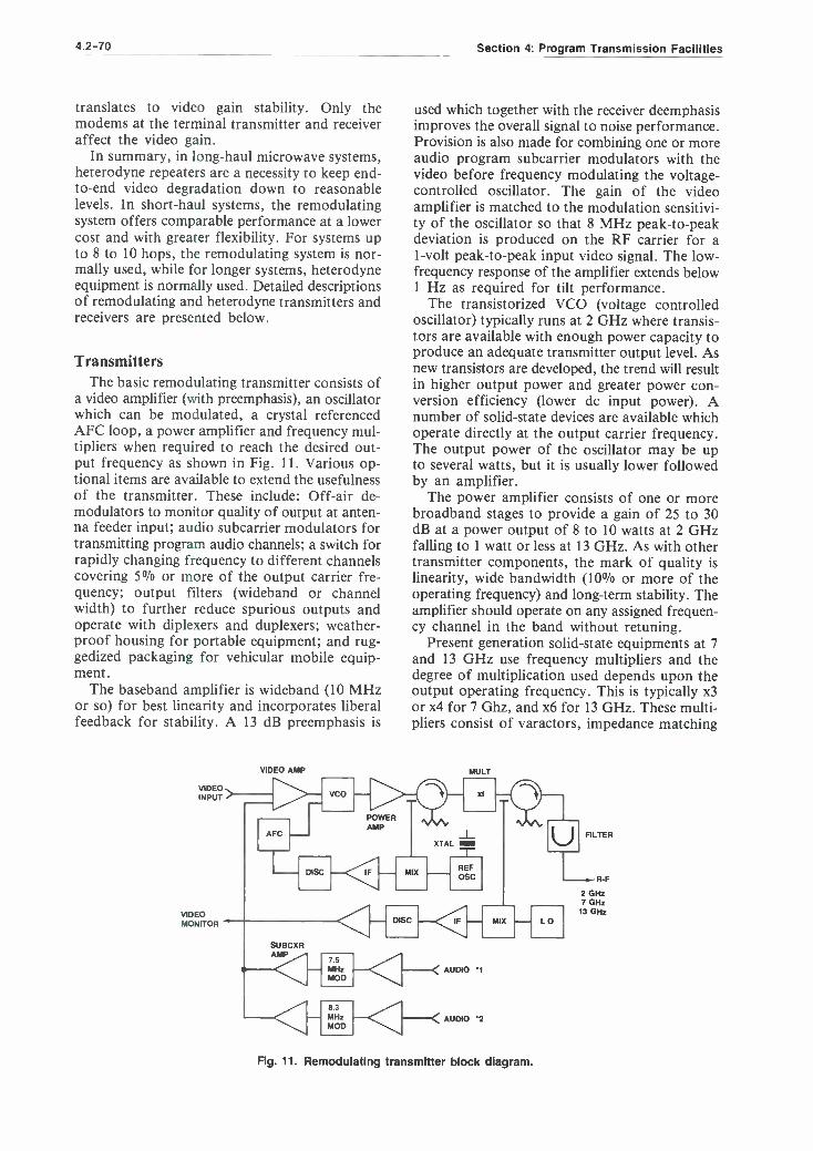
4.2 -70 Section 4: Program Transmission Facilities
translates to video gain stability. Only the modems at the terminal transmitter and receiver affect the video gain.
In summary, in long -haul microwave systems, heterodyne repeaters are a necessity to keep end - to -end video degradation down to reasonable levels. In short -haul systems, the remodulating system offers comparable performance at a lower cost and with greater flexibility. For systems up to 8 to 10 hops, the remodulating system is nor- mally used, while for longer systems, heterodyne equipment is normally used. Detailed descriptions of remodulating and heterodyne transmitters and receivers are presented below.
Transmitters The basic remodulating transmitter consists of
a video amplifier (with preemphasis), an oscillator which can be modulated, a crystal referenced AFC loop, a power amplifier and frequency mul- tipliers when required to reach the desired out- put frequency as shown in Fig. 11. Various op- tional items are available to extend the usefulness of the transmitter. These include: Off -air de- modulators to monitor quality of output at anten- na feeder input; audio subcarrier modulators for transmitting program audio channels; a switch for rapidly changing frequency to different channels covering 5% or more of the output carrier fre- quency; output filters (wideband or channel width) to further reduce spurious outputs and operate with diplexers and duplexers; weather- proof housing for portable equipment; and rug - gedized packaging for vehicular mobile equip- ment.
The baseband amplifier is wideband (10 MHz or so) for best linearity and incorporates liberal feedback for stability. A 13 dB preemphasis is
VIDEO INPUT
VIDEO MONITOR
VIDEO AMP
used which together with the receiver deemphasis improves the overall signal to noise performance. Provision is also made for combining one or more audio program subcarrier modulators with the video before frequency modulating the voltage - controlled oscillator. The gain of the video amplifier is matched to the modulation sensitivi- ty of the oscillator so that 8 MHz peak -to -peak deviation is produced on the RF carrier for a 1 -volt peak -to -peak input video signal. The low - frequency response of the amplifier extends below 1 Hz as required for tilt performance.
The transistorized VCO (voltage controlled oscillator) typically runs at 2 GHz where transis- tors are available with enough power capacity to produce an adequate transmitter output level. As new transistors are developed, the trend will result in higher output power and greater power con- version efficiency (lower dc input power). A number of solid -state devices are available which operate directly at the output carrier frequency. The output power of the oscillator may be up to several watts, but it is usually lower followed by an amplifier.
The power amplifier consists of one or more broadband stages to provide a gain of 25 to 30 dB at a power output of 8 to 10 watts at 2 GHz falling to 1 watt or less at 13 GHz. As with other transmitter components, the mark of quality is linearity, wide bandwidth (10% or more of the operating frequency) and long -term stability. The amplifier should operate on any assigned frequen- cy channel in the band without retuning.
Present generation solid -state equipments at 7 and 13 GHz use frequency multipliers and the degree of multiplication used depends upon the output operating frequency. This is typically x3 or x4 for 7 Ghz, and x6 for 13 GHz. These multi- pliers consist of varactors, impedance matching
MULI
AFC
DISC
POWER AMP -I-
XTAL NM T H REF OSC
AUDIO '1
AUDIO '2
LO
FILTER
Ths.- R-F
2 GHz 7 GHz
13 GHz
Fig. 11. Remodulating transmitter block diagram.

Chapter 2: Microwave Engineering for the Broadcaster 4.2 -71
circuits, cavities, and filters to efficiently operate over a wide band of frequencies with minimum spurious output signals. No tuning is required to cover up to 10 assigned frequency channels in one of the three operating bands. Typical power out- put from the varactor multiplier is 1 to 2 watts at 7 GHz and 0.8 watts at 13 GHz. At the pres- ent time, operating frequencies of solid -state com- ponents are increasing so that the need for fre- quency multipliers will not exist for any frequen- cy band in the near future, as they are not now required at 2 GHz.
Two approaches for AFC are common: Fig. 11 illustrates a crystal -controlled source which feeds one side of a mixer. The other side of the mixer is fed with a sample of the transmit- ter frequency. The mixer output is an IF signal which is amplified and demodulated by a tern - perature compensated discriminator. The dc out- put from the discriminator is the carrier frequency error voltage which, when applied through a dc amplifier to the VCO, keeps it on its assigned frequency. A more state -of -art approach uses a phase -locked oscillator as the microwave source. Here a microwave IC divider samples the oscil- lator output directly at 2 GHz. The output of the divider is at a frequency where standard PLL IC's and techniques can be used to lock the oscillator to a crystal reference. The phaselock approach involves less hardware and is thus less expensive.
The off -air monitor is essentially a microwave receiver which demodulates a sample of the trans- mitter output signal for monitoring. To be of maximum value as a transmitter test tool, the monitor signal should be of high quality even though this approach is slightly more expensive than slope detectors and other lower cost devices which are sometimes used.
The frequency switcher shifts the operating bias on the oscillator to change its frequency and, when AFC is used, switches crystals in the reference oscillator. Since all circuits are wideband, no tun- ing is necessary when frequency is changed.
The transmitter output filter is used when the transmitter is diplexed with another transmitter or duplexed with a receiver, or to reduce spurious levels. The filter may be broadband covering 5% or more of the spectrum, or narrow band cover- ing a single assigned channel.
For portable applications, a weatherproof housing is required which is easily fitted, with an antenna, to a tripod. If remote control is used, special wiring and a connector are installed for mating with the remote control cable.
Equipment for mobile applications must be packaged in a rugged manner to withstand the high degree of shock and vibration experienced in most vehicles. Also size and weight become more important so special precautions must be taken to keep the high density packaged corn-
ponents from overheating. To prevent interference to or from broadcast
microwave equipment, special precautions must be taken for RFI filtering and shielding. The total unit is usually enclosed in an RFI resistant case with critical circuitry completely shielded. Addi- tionally, all input and output electrical connec- tions must be RFI filtered. Without these pre- cautions, considerable difficulty can be expected, since broadcast microwave equipment often oper- ates in close proximity to high powered trans- mitters.
Receivers All TV microwave receivers are typically super-
heterodyne with a 70 MHz IF amplifier as shown in Fig. 12. For broadcast work, the local oscillator and mixer should be broadband to eliminate the need for tuning when switching to a variety of different frequencies.
Mixers are usually balanced mixers and often double balanced. If no low -noise amplifier (LNA) is used, the mixer determines the noise figure of the receiver which is in turn largely dependent on the diodes used. Noise figures of 8 dB at 2 GHz rising to 9 dB at 13 GHz are common. The mixer function is to produce an IF frequency by generating the difference between the local oscillator frequency and the received carrier frequency.
For superior noise performance and fade margin, a low -noise amplifier may be added to the receiver design (as in the figure). Using a LNA, receiver noise figures of 1.5 dB at 2 Ghz rising to 3 dB at 13 GHz are achieveable. Modern LNA designs are based on Ga -As (Gallium Arsenide) FETS. Previously, tunnel diode designs were used at 7 and 13 GHz while bipolar tran- sistors were used at 2 GHz. The gain of these LNA's is typically 15 to 20 dB.
LNA's are also available separately for use out- side the receiver. In this case, they are often mounted near the antenna and are provided with a weatherproof housing. In this case, the loss of the transmission line is eliminated and the system improvement is further increased. Another poten- tial application of the low noise amplifier is be- tween two back -to -back dishes operating as an active repeater. FCC action on this configuration is imminent. The low noise amplifier is a useful tool to the microwave design engineer, and its use in the system should not be overlooked.
The local oscillator carrier is usually crystal controlled to 0.005% or better of the output fre- quency. This eliminates the need for receiver AFC. Fundamental oscillators are usually used, but lower frequency oscillators followed by multipliers are occasionally used as well. For fre- quency agile equipment, up to 10 switch -selectable

4.2 -72 Section 4: Program Transmission Facilities
DISC EO
VIDEO .AMPP
VIDEO
AUDIO ' 1
AUDIO 2
MAIN
U SUBCXR AMP
PRE
IF
I F FILTER
V NOTCH FILTERS
75 MHz
DEMOD
AUDIO AMPS
8.3 MHz
DEMOD
_L XTAL T
Fig. 12. Receiver block diagram.
crystal references may be used, or a suitable syn- thesizer employed.
The 70 MHz IF preamplifier is often mechan- ically integrated with the mixer to achieve best overall noise figure of the receiver. The pream- plifier typically has 25 dB gain and is 50 to 60 MHz wide.
Optimum receiver noise performance is achieved when the minimum necessary bandwidth is used. This is typically 30 MHz to the 3 dB points for TV transmission. However in many metropolitan areas, frequency congestion is pushing usage to 20 MHz wide IF band widths. Since the basic IF amplifier circuits are 50 to 60 MHz or more wide, a lumped constant filter located between the preamplifier and the main IF is employed to reduce the noise bandwidth of the receiver to 30 MHz. The characteristics of this filter must be carefully controlled for good phase and amplitude linearity.
The main IF amp follows the filter and pro- vides typically 65 dB of gain. In both pre and main IFs, discrete common -base transistor design had previously been used. This effectively isolates the transistor characteristics from the overall amplifier performance characteristics which are determined primarily by the interstage coupling circuits. With this design approach, the receiver characteristics are essentially independent of the transistor characteristics which may vary widely with temperature. However, current approach is to use special purpose IC's or RF modules to pro- vide IF gain. The output level of the IF is typically + 5 dBm. The input microwave level to a typical receiver may vary from - 25 to - 80 dBm dur- ing fading conditions. Since + 5 dBm output is required, the gain needed varies from 30 dB to 85 dB. In order to keep the output constant, 60 dB of AGC is typically used to regulate the 90 dB gain in the two IF amplifiers between 40 and
IMAGE FILTER
LOW NOISE AMP (OPTION)
CHANNEL FILTER
< R F
2 GHz 7 GHz
13 GHz
90 dB. Since portable and mobile equipment operate over wide ranges of distance, it is impor- tant that receivers have at least 60 dB of AGC.
The limiters are an essential part of an FM receiver because they effectively eliminate the ef- fects of AM variations on threshold performance. Typically 20 dB of limiting is used.
The discriminator demodulates the FM signal back to video. In a wideband TV system, it is important to keep the discriminator linear over a wide bandwidth, typically ± 5 MHz or more about the center 70 MHz IF frequency. Non - linearity will produce distortion and noise on the signal by increasing intermodulation between various components of the TV signal.
The video amplifier brings the discriminator output signal back up to one volt. It also includes a deemphasis network which is exactly matched to the transmitter preemphasis network so that an overall flat frequency response is achieved through the system. The video amplifier includes a low pass filter to reduce the level of the audio subcarriers at the video output. While the degree of audio subcarrier rejection is not extremely im- portant in TV microwave signals, it is typically 30 to 40 dB below peak video levels. A high degree of feedback is used in the video amplifier to achieve maximum stability.
The preselect filter at the receiver input is used to improve selectively, prevent local oscillator radiation, and suppress image frequencies. It typically consists of five or more filter selections designed and tuned to cover several channels in switch tunable systems or a single channel in fixed signals. The passband characteristics must be closely controlled to avoid phase non -linearities in the system.
The same comments made for the transmitter regarding portable and vehicular applications apply to the receiver.

Chapter 2: Microwave Engineering for the Broadcaster 4.2 -73
Basic Heterodyne TV Microwave The receiver in a heterodyne system is almost
identical to the remodulating receiver already discussed, the only difference being that the out- put is taken at 70 MHz from the IF amplifier and connected to the heterodyne transmitter. A second IF output may be used to feed an optional 70 MHz demodulator (limiter, discriminator and video amplifier) if a video drop is desired at the hop.
The heterodyne transmitter block diagram is shown in Fig. 13. It consists of an IF amplifier and a microwave source both of which feed an up converter mixer. The source is similar to that used in the remodulating transmitter except it need not be modulated. The mixer heterodynes the 70 MHz IF input signal up to a microwave signal ± 70 MHz different from the source fre- quency depending upon the sideband selected. The sideband select filter passes the desired side - band while rejecting the undesired sideband and source frequency.
VIDEO
AUDIO
AUDIO
VIDEO
MICROWAVE RECEIVER
70 MHz
FM DEMOD
FOR REPEATER
70 SERVICE MHz - -
\ TERMINAL
70 MHz F -M MOD
HP LP FILTER
IF AMP
A microwave power amplifier is then used to restore the level of the signal to its desired value. Impatt diode (Avalanche diode) reflection ampli- fiers have been the norm and are still being pro- duced, but the current move appears to be to Ga- As FET power amplifiers.
At a repeater the 70 MHz IF input to the trans- mitter comes from the receiver IF output at a level of + 5 dBm. If the heterodyne transmitter is used at a terminal station, the video signal first modulates a 70 MHz FM transmitter (modulator) which then feeds the transmitter.
Power Supplies Whether remodulating or heterodyne, micro-
wave equipment uses several different voltages to power the various active circuit components. These are usually low voltages in the 12 to 35 range that must be highly regulated and filtered for best performance. The power supply func- tion is to convert the ac or dc main supply voltage to those required in the equipment.
UP CONVERTER
FREQUENCY MULTIPLIERS
SIDE BAND SELECT FILTER
XTAL OSCILLATOR- MULTIPLIER
ALARM! CONTROL
Fig. 13. Heterodyne transmitter block diagram.
BATTERY EQUIPMENT
OPERATED
LOW VOLTAGE
ALARM
CHARGER ALARM
AC }- CHARGER 1_40_, PRE- REGULATORr INVERTER LINE
A -C LINE
24 OR 48V BATTERY
TRANSFORMER
-r
DIRECT A -C LINE OPERATED EQUIPMENT
)--1 RECTIFIER
REGULATOR
REGULATOR
RECTIFIER
Fig. 14. Power supply block diagram.
RF
POWER AMP
D -C OPERATING VOLTAGES

4.2 -74 Section 4: Program Transmission Facilities
Fig. 14 is a block diagram of a typical power supply system. AC units consist of a transformer and rectifiers to obtain the unregulated operating voltages. Various types of transistor regulators are used to keep the operating voltages within a narrow range of variation. In dc units, the bat- tery voltage is first converted to ac by a chopper or inverter after which operation is similar to the ac. Good designs usually employ protection cir- cuits on both input and outputs to protect the power supply from surges, load short circuits, and lightning. The power supply may be separate from the transmitter or receiver or it may be built in.
Subcarriers In addition to carrying the video traffic, a
microwave link can carry additional information above the video portion of the baseband. As the NTSC video bandwidth extends to 4.2 to 4.5 MHz, the area above 4.5 MHz, after allowing a suitable guard band, is available for other use. Four different uses are made of this baseband spectrum: Program audio subcarriers (multiple); engineering order wire; supervisory signals (alarms); and continuity pilot. In all uses, the deviation is generally 20 dB below the peak video deviation of 4 MHz.
The program audio subcarriers are generally modulated 75 kHz peak deviation at a 1 kHz test tone. Maximum audio bandwidth is almost uni- versally 15 kHz. From Carson's rule the in- formation bandwidth is thus 180 kHz. To allow adequate filtering of one subcarrier from the next, subcarriers are generally spaced at least 600 kHz apart (though occasionally a 400 kHz spacing is used.) Moreover, successive subcarriers are spaced at successively larger distances apart. This avoids a multiple difference beat of 600 kHz in the video baseband.
Up to four audio subcarriers are commonly used. But the more subcarriers used, the greater receiver bandwidth required, with its trade -offs. When 25 MHz wide channels (7 and 13 GHz bands), the four subcarriers are often located at 6.2, 6.8, 7.5 and 8.3 MHz. If 17 MHz wide chan- nels are used, (2 GHz band) the four subcarriers might be located at 5.8, 6.2, 6.8 and 7.5 MHz. However, such a four subcarrier system in a 17
MHz bandwidth will show compromises in audio and video quality. Occasionally a subcarrier at 4.83 MHz will be used. However, this generally requires more severe video filtering, and the resul- tant degradation of video performance. The 4.83 MHz subcarrier is generally used in ENG systems (see Section 6), where a narrow IF filter is desirable due to transmitter power limitations and band congestion.
Often a single- side -band suppressed- carrier supervisory and control system is added to the baseband. If less than four subcarriers are used, this SSB system might be located at one of the above mentioned subcarrier frequencies. In four subcarrier systems, the SSB system might be located at 8.59 or 9.023 MHz. The supervisory and control system can include both an engineer's order wire and remote repeater alarming. The order wire allows two way communication among the terminals and the repeaters. The alarming allows automated fault reporting from these unat- tended repeater locations. The requirements for "partyline" transmission from multiple sites forces the use of a suppressed carrier, avoiding carrier beats which would otherwise occur.
In addition, a continuity pilot may be includ- ed in the baseband spectrum. Generally the pilot is the highest frequency in the baseband; 8.59 and 9.023 MHz are commonly used.
Descriptions of program audio modulators and demodulators are next presented. Note that depending on manufacturers and model, the pro- gram audio modulator and demodulator might be packaged separately or be integral to the microwave transmitter or receiver.
The subcarrier modulator is actually an FM transmitter operating in the range of 4.83 to 8.3 MHz. The subcarrier oscillator is generally fre- quency stabilized. Previous techniques had in- cluded AFC for the oscillator using a built -in FM discriminator as the frequency reference. Current practice is to phase lock the oscillator to a crystal reference using IC phase -lock components. Usual- ly 75 µs preemphasis is employed in the audio circuit.
The subcarrier demodulator is similarly a FM receiver operating in the range of 4.83 to 8.3 MHz. These demodulators are available fixed tuned to one subcarrier frequency (analogous to a TRF receiver) or frequency agile, able to be tuned to several subcarrier frequencies (the super- heterodyne approach). In either case, the "RF" or "IF" filters must be sharp enough to reject adjacent subcarriers as well as the 20 dB stronger video signal.
Due to residual non -linearity in the microwave modulator and demodulator, as well as in the path, sometimes cross modulation of the video appears on the demodulated audio. The most an- noying characteristic is a 15.7 kHz buzz caused by the video horizontal scanning frequency. Sub - carrier demodulator manufacturers often include a 15.7 kHz notch in their audio processing cir- cuitry to suppress this tone. This notch require- ment is difficult, as little attenuation at 15.0 kHz (top of the audio band) is allowed. In addition, 75 µs deemphasis and perhaps, noise low -pass filtering above 15 kHz is included in the audio circuitry.

Chapter 2: Microwave Engineering for the Broadcaster 4.2 -75
Audio output level is generally + 9 to + 18 dBm, at a balanced 600 ohms; for multiple out- puts a low- impedance option is sometimes available.
POWER PLANTS
Primary Power and Back -up With improvements in equipment and systems
engineering, the reliability of the main power source becomes more important. With solid state equipment which requires low power and voltages, batteries are the most popular form of standby power. If prolonged commercial power failures are anticipated, engine -generator sets are used to recharge the batteries. In some remote areas, gas fueled thermoelectric generators are used and solar power is now becoming an eco- nomic alternative except in the most northerly states where the necessary standby battery capaci- ty becomes prohibitive.
Industrial lead -acid batteries are most often used. To give strength to the plate structure the lead is alloyed with calcium, antimony or sele- nium, and this gives each cell certain advantages or disadvantages depending on application.
Currently, industrial lead- calcium or lead - antimony acid batteries are most often used. Both types are reliable and the choice is often one of personal preference. The one advantage of lead calcium is that equalizing charges are not required which reduces maintenance. The float charge volt- age is 2.15 volts per cell for lead- antimony, 2.2 volts per cell for lead -calcium, and 2.23 volts per cell for lead -selenium. Batteries should be in- stalled in well -ventilated areas to reduce the pos- sibility of explosion from escaping hydrogen gas. Battery banks usually consist of 12 to 24 cells (24 to 48 volts) and the positive terminal is grounded. Cell voltage typically varies over a range of 1.75 to 2.35 volts when completely discharged and when at maximum charging rate. The communi- cation equipment must be capable of accepting this variation. Battery size is usually selected for a minimum 8 -hour capacity with 24 -hour capacity being about the economic limit. To arrive at the minimum ampere -hour capacity (AH) for a given standby period, the average station load (A) should be multiplied by the hours of standby re- quired (H), typically 8 -12.
To arrive at the minimum charger capacity (C) to recharge in R hours, the average station load should be multiplied by the factor:
A + H x A x 1.1 C amperes [16]
R
When H = 8 and R = 24 this factor is 1.37. R should not be less than 2.5 times H.
Since charger failure would lead to station failure after H hours, a key repeater could re- quire a duplicated charger for full protection. In this case each charger need only have a capacity equal to the station load A rather than C as de- rived above.
Present day batteries are quite reliable and re- quire little attention for many years. Batteries are also effective filters to protect solid state equip- ment from power line surges, and act as a very large capacitor, so reducing ripple from the charger.
Battery chargers operate from standard com- mercial power and actually provide the power to the equipment with the battery floating as a stand- by device. Good chargers should incorporate pro- tective devices to limit charging current and to protect against line surges and duplicated chargers should be designed to share the load. Alarms for charger and line voltage failure should also be available. Purchase of batteries and chargers from the same source of supply is recommended to in- sure compatibility.
Batteries and charges are sound investments which will add many hours of operating time to the average microwave system.
When diesel generators are the primary source of power they should not be run at less than 75% of rated load (after allowing for any de- rating
Fig. 16. A fixed solar powered TV station in Oman with a wind powered generator.
(Courtesy of Solarex Corporation)

4.2 -76 Section 4: Program Transmission Facilities
due to altitude). This prevents oiling -up of the engines.
Solar power using photo -voltaic cells is attrac- tive as there are no moving parts requiring maintenance. However the batteries required to maintain the supply during periods of darkness or heavily -clouded weather (which could be several days in some areas) can be the most ex- pensive item in a solar installation. It may pay to have a small generator which can be cut in after 48 hours rather than a battery to give, say, six days standby when that capacity may only be required once or twice a year. The small generator can also power lighting and test gear during a maintenance visit to the site.
FREQUENCY PLANNING Frequency coordination has been primarily a
local case -by -case selection process through cooperation of the respective chief engineers. Most areas, through the local chapter of the Society of Broadcast Engineers (SBE), maintain an up -to -date log of existing licences.
Ideally, frequency planning for future growth should follow the following basic parameters:
A. Multi -Hop System: High -Low Plan
Tx @Ch 1 Tx @Ch IO Tx @Ch 1
Site I Site II Site III
Simplex System -One Way
B. Multi -Hop System: Duplex -Two Way
Tx @ Ch 1 Rx @ Ch 1 Tx @ Ch 10 Rx @ Ch 10
1 Tx@ChIO Rx @ Ch ]0 Rx@Chl Tx @ Ch
Site I Site II Site III
Future growth allows a second channel addi- tion, diplexed on the same antenna system, with alternate channel selections.
With the High /Low Plan, channel additions can expand up from low end and down from high end.
Basic rules with standard transmitter and receiver designs sharing the same antenna network are:
Diplex- Channel Expansion -Same Direction - Alternate Channels
Duplex -Channel Expansion -Two Directions - Minimum two clear channels between transmit- ter and receiver at same end. When more than one transmitter is multiplexed onto a feeder, any receiver on that feeder must avoid 2A -B inter - modulation products; this can be done by using even channels for transmitters and odd channels for receivers.
Cross polarization can be employed to inter- leave the channel plan, but care must be exer- cized in controlling the respective bandwidths through modulation control and RF /IF response.
Frequency Re -Use Microwave antenna discrimination provides a
degree of isolation that very often allows the re- use of the same channel as the same or a nearby site a number of times.
The EIA Interference Criteria, "Telecom- munications Systems Bulletin 10D," specifies a carrier to interference (C /I) ratio of 60 dB. This is ideal, but in many cases very difficult to realize. Acceptance of a lesser C/I ratio has worked suc- cessfully in many cases.
Lowering the C/I ratio will raise the effective noise level and hence reduce the fade margin. Given a threshold of 80 dBm, say, the noise level will be appropriately 90 dBm and in- terference at 90 dBm will raise the threshold to 77 dBm. This may be acceptable in many cases.
Assume a well- designed path from Site A to Site B has, by design, a 40 dB fade margin from normal receive carrier level to Threshold- defined as 37 dB Video S /N. If another co- channel (same frequency) transmitter with same power output and antenna size is located at Site A, but aimed in another direction and the side lobe of the new antenna is only 50 dB down, relative to main beam, a 3 dB increase in the noise floor of the original receiver would be expected and undesir- able. If, however, the side lobe can be made greater than 50 dB down, a lesser noise floor in- crease would be expected. Antenna patterns typically describe a worst -case peak envelope and in practice, the nulls can be well below the envelope and provide essentially no contribution to the original system noise floor. Many systems have been successfully built along this line. Fading over respective paths would be identical and the two systems could exist on the same frequency.
Same site re -use of receiver frequency can be considered in the same fashion with care exer- cized relative to fading differential.

Chapter 2: Microwave Engineering for the Broadcaster 4.2_77
FCC LICENSING
FCC Application All broadcast microwave systems, portable or
in fixed station operation, must be licensed through the FCC. The application is filed on FCC Form 313, with the pertinent characteristics and Type Acceptance Identification Number provided by the respective manufacturer.
Frequency coordination for clearance of the ap- plied for frequency is the responsibility of the local area engineers. In contrast, licensing by Common Carriers, Industrial Service and CARS Band operators is supported by formal frequen- cy coordination studies. The applicant provides detail analysis of use of the applied for frequen- cy in the area with supporting technical details as to the acceptance of the use.
Broadcast engineers should be aware and care- ful when applying for channels in the 12.7 to 13.25 GHz Band. This band is shared with CARS -Cable TV Operations, and is in wide ser- vice in most areas.
The details in Form 313 are straight forward. However, some confusion may arise on Item 8 treating transmitter output. Subsection 8.B.1 is the typical output of the specific transmitter. Subsection 8.B.2 is the antenna input power and represents the actual typical power expected to reach the transmitting antenna after subtracting the losses expected from the length of connect- ing coaxial or waveguide transmission line. Subsection 8.B.3 is the Effective Radiated Power (ERP) actually transmitted and is the input power raised by the antenna gain. Subsection 8.0 is the Emission Designator, 17,000 F9 at 2 GHz and 25,000 F9 at 7 and 13 GHz.
Portable frequency agile transmitters are typ- ically licensed for all the channels that they can provide. For example, at 2 GHz, all seven chan- nels are submitted on the single license applica- tions.
Broadcasters and others using this Handbook should refer to the FCC Rules and Regulations and to their attorneys for complete, up -to -date information.
REFERENCES 1. Alvira, A., & Corbell, I. T., "Reliable Micro-
wave System Parameters," Power Apparatus and Systems, Institute of Electrical and Elec- tronics Engineers, December 1955, pp. 110- 1107.
2. EIA Standard RS- 250 -B, Electrical Perfor- mance Standards for Television Relay Facili- ties, Electronics Industries Association, Washington, D.C., September 1976.
3. Television Signal Analysis, Second Edition, American Telephone and Telegraph Com- pany, Long Lines Department, April 1963.
4. C.C.I.R. Documents of the Fifteenth Plenary Assembly, Geneva, Switzerland, 1982.
5. The Lenkurt Demodulator, Second Edition, Lenkurt Electric Company, San Carlos, Cal- ifornia, 1966.
6. Reference Data for Radio Engineers, Fifth Edition, International Telephone and Tele- graph Corporation.
7. Planning and Engineering of Radio Link Paths, Sixth Edition, Siemens and Halske Aktiengesellschaft, Munich, Germany, March 1961.
8. Egli, J. J., "Radio Relay System Engineer- ing," Proceedings of the IRE, January 1953.
9. Hogg, D. C., "Statistics on Attenuation of Microwave by Intense Rain," Bell System Technical Journal, November 1969.
10. Jakes, W. C., Jr., "A Theoretical Study of An Antenna -Reflector Problem," Proceed- ings of the IRE, February 1953.
11. Engineering Consideration for Microwave Communications Systems, by Lenkurt Elec- tric Company, San Carlos, California, 1981.
12 . N.A.B. Engineering Handbook, Sixth Edi- tion, Section 21, I.T. Corbell, 1975.


4.3
Satellite Earth Stations James Fitzgerald Vice President, Earth Station Services Comsearch, Inc. Reston, Virginia
INTRODUCTION In less than a decade, satellites have become
an essential part of the broadcasting industry. The rapid fall in the cost of satellite transmission has made satellites the vehicle of choice for program distribution. As the cost of satellite transmission continues to fall, we are fast approaching a time when many broadcasters will not only receive but also transmit programming by satellite as a natural extension of their role as communication centers. The local broadcaster may on a "shared use" basis transmit teleconferences for local cor- porations, distribute programming for LPTV net- works or distribute its own "superstation" pro- gram material.
There are at this time two major developments that are changing the nature of satellite broad- casting. One is the introduction of the 14/12 GHz transmission, which provides channels with less interference from terrestrial microwave systems. The other is the introduction of 2 ° satellite spac- ing in the 14/12 GHz band and eventually in the 6/4 GHz band as well.
Satellite communication still has two primary advantages over terrestrial distribution- commu- nication cost is independent of distance and many points can be served with a relatively small in- vestment in terminal equipment. These charac- teristics make satellites an ideal means for delivery of broadcast programming over vast areas, such as the United States.
SYSTEM DESCRIPTION A satellite communication system consists of
a transmitting earth station, a satellite, (with a receive antenna, transponder and transmit anten- na,) and a receiving earth station (Fig. 1 and 2). Since the characteristics of the satellite com- ponents determine the requirements of the earth systems, the analysis must begin with the satellite.
Satellite Frequencies, Channeling and Polarization
Satellites used for broadcast program relay are in an orbit 22,282 miles above the equator. In this orbit a satellite travels around the earth in exactly 24 hours, so that it appears stationary at a fixed point over the earth (geosynchronous).
Like a microwave relay on earth, the satellite receives and transmits at different frequencies to prevent interference between incoming and out- going signals. Current broadcast satellites oper- ate in the C band (also known as the 6/4 or 4/6 GHz band) or the Ku band (also known as the 12/14 or 14/12 GHz band). C band uses uplinks from 5.925 to 6.425 GHz and downlinks from 3.7 -4.2 GHz. Ku band uses uplinks from 14.0 -14.5 GHz and downlinks from 11.7 -12.2 GHz.
The satellite bandwidth is divided into chan- nels. In the C band, 36 MHz channels have been standard (with two 2 -MHz guard bands, so that
4.3 -79
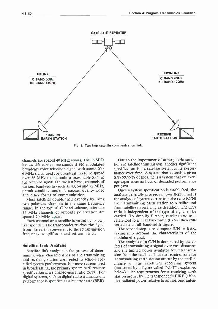
4.3 -80
UPLINK
C BAND 6GHz Ku BAND 14GHz
Section 4: Program Transmission Facilities
SATELLITE REPEATER
DOWNLINK
C BAND 4GHz Ku BAND 12GHz
TRANSMIT EARTH STATION
Fig. 1. Two hop satellite communication link.
channels are spaced 40 MHz apart). The 36 MHz bandwidth carries one standard FM modulated broadcast color television signal with sound (the 6 MHz signal used for broadcast has to be spread over 36 MHz to maintain a reasonable S/N in the received signal.) In the Ku band, channels of various bandwidths (such as 43, 54 and 72 MHz) permit combinations of broadcast quality video and other forms of communication.
Most satellites double their capacity by using two polarized channels in the same frequency range. In the typical C band scheme, alternate 36 MHz channels of opposite polarization are spaced 20 MHz apart.
Each channel on a satellite is served by its own transponder. The transponder receives the signal from the earth, converts it to the retransmission frequency, amplifies it and retransmits it.
Satellite Link Analysis Satellite link analysis is the process of deter-
mining what characteristics of the transmitting and receiving station are needed to achieve spe- cified system performance. For most systems used in broadcasting, the primary system performance specification is a signal -to -noise ratio (S /N). For digital systems, such as digital radio transmission, performance is specified as a bit error rate (BER).
RECEIVE EARTH STATION
Due to the importance of atmospheric condi- tions in satellite transmission, another significant specification for a satellite system is its perfor- mance over time. A system that exceeds a given S/N 99.99% of the time is a system that on aver- age experiences an hour of degraded performance per year.
Once a system specification is established, the analysis generally proceeds in two steps. First is
the analysis of system carrier -to -noise ratio (C /N) from transmitting earth station to satellite and from satellite to receiving earth station. The C/N ratio is independent of the type of signal to be carried. To simplify further, carrier -to -noise is referenced to a 1 Hz bandwidth (C /No) then con- verted to a full bandwidth figure.
The second step is to compute S/N or BER, taking into account the characteristics of the modulated signal.
The analysis of a C/N is dominated by the ef- fects of transmitting a signal over vast distances and the limited power available for retransmis- sion from the satellite. Thus the requirements for a transmitting earth station are set by the perfor- mance of the satellite's receiving system (measured by a figure called "G /T ", explained below). The requirements for a receiving earth station are set by the transponder's EIRP (effec- tive radiated power relative to an isotropic anten-

Chapter 3: Satellite Earth Stations
INPUT SIGNAL
MODULATOR
RF AMPLIFIER
OUTPUT SIGNAL
EXCITER
TRANSMIT EARTH STATION
TRANSLATOR
RF AMPLIFIER
SATELLITE REPEATER
RECEIVER
RECEIVER
LNA
RECEIVER EARTH STATION
0
Fig. 2. Simplified block diagram satellite communication system.
4.3 -81
ANTENNA
UPLINK
SATELLITE ANTENNA
DOWNLINK
ANTENNA

4.3 -82 Section 4: Program Transmission Facilities
na.) The G/T and the EIRP levels vary by loca- tion. "Footprint" maps (Fig. 3) show the con- tours of G/T and effective EIRP. These foot- prints vary by satellite and by transponder.
For either an unplink or a downlink, C /No is computed using an equation like the following:
(C/o) = EIRP + (G/T) + 228.6 - Lfs - La [11
Where: EIRP =
G/T = 228.6 =
Lfs = La =
effective isotropic radiated power from the transmitter (dBw) figure of merit (see below) (dB) Boltzmann's constant (dBw -Hz) Free space loss (dB) Atmospheric loss (dB)
Of these figures, EIRP is the sum of antenna power and antenna again. Power at the antenna is a specification of the amplifier feeding the antenna. In the case of the earth station, amplifier power is on the order of 500 W (27 dBW) from a high -powered amplifier (HPA) for video ser- vices. The satellite power, supplied by solar panels, is limited to 5 -10 W (7 to 10 dBW). Gain depends on the efficiency of the antenna and is proportional to the square of the frequency of transmission and the aperture area of the anten- na. The larger the antenna, the larger the gain. EIRP is easily computed for a transmitting sta- tion given the power at the feed flange and anten- na gain (from the manufacturer). Satellite EIRP is available from a footprint map.
G /T, also called "figure of merit ", is a measure of the ability of a receiving system to
amplify very weak signals, such as those of a transmitter 22,300 miles away, over background noise. The "G" is antenna gain. The "T" is a noise temperature, which is specified in degrees Kelvin for equipment used in satellite communica- tions. For purposes of satellite link analysis, all noise is referred to an equivalent level of ther- mal noise, that is, the noise caused by random motion of electrons. As noted above, a footprint map of G/T for the satellite transponder supplies the figure used in calculating uplinks.
For downlinks, the gain figure is obtained from manufacturing specifications. The noise temper- ature, T, of the receiving earth station is the sum of antenna noise temperature and the noise temperature of the system's electronics, as shown in the following equation:
Ts = Gfeed
Where: Ts =
Ta = Tina =
Treceiver =
Gfeed =
Gina =
Ta + Tina / Gfeed X Gina
+ Treceiver / [2]
total system noise temperature ( °K) antenna noise temperature ( °K) noise temperature of the LNA ( °K) noise temperature of the receiver ( °K) gain of the device coupling feed to LNA (dB) gain of the LNA (dB)
Antenna noise temperature, Ta, depends on the elevation of the antenna, since an antenna point- ing to cold space faces less noise than one angled
Fig. 3. Footprint showing assumed satellite EIRP in dBW at 4 GHz. (Figure actually shows average EIRP of RCA SATCOM f1 at 135 °W for transponders 3, 7, 11, 15, 19 and 23)
(Courtesy J. Searcy Hollis, Scientific Atlanta, Inc.)

Chapter 3: Satellite Earth Stations
50
40
30
20
10
0
COMPUTED DATA
0 10 20 30 40 50 60 70
ELEVATION ANGLE (DEGREES)
80 90
4.3 -83
Fig. 4. Typical variation of the noise temperature of a satellite antenna as a function of elevation angle. (Courtesy J. Searcy Hollis, Scientific Atlanta, Inc.)
closer to the warm earth. Fig. 4 shows a typical relationship between antenna noise temperature and elevation angle.
Of the remaining terms in equation [2], only Ti should make a difference. An LNA should be selected with a gain sufficient to overcome ef- fects of noise temperature in the components that follow it.
The constant 228.6 in equation [1] is Boltzmann's constant (1.38 x 10 23 W / °K -Hz) ex- pressed in decibels. This universal constant relates the noise temperature in G/T to power.
Free space loss, Lfs, can be expressed (in watts) as:
L f s = (4 x n x f x D / C)
Where: f = frequency, Hertz D = distance traveled, meters C = the speed of light (2.99 x 10⁸ meters/
second)
The final term in equation [1] refers to at- mospheric loss. This term can be neglected under most circumstances, particularly with C -band (6/4 GHz) systems. Ku band (14/12 GHz) systems are more likely to be affected by intense rain and heavy clouds. Atmospheric loss for all bands also increases with lower elevation of the earth sta- tion, since the station must look through more of the atmosphere.
Equation [1] calculates a single link from earth to satellite or from satellite to earth. To compute a two -hop link (earth to satellite to earth), the individual hops are calculated, then the two
figures are combined by power addition. For power addition, decibel figures are converted back to ratios and then summed using the formula:
C/No = 1
1 1
C/N + C/Nod
The result is then reconverted to decibels. In this type of summation, the resulting noise level is higher than either of the links considered alone.
Types of Signals Carried There are a number of types of signals that a
broadcaster will encounter on satellite:
Full transponder FM video. This is a standard broadcast signal, including color and sync tips, using 36 MHz of bandwidth, in C -band systems.
Half transponder FM video is a video signal that uses 18 MHz bandwidth (whether or not the transponder actually has a 36 MHz bandwidth). Both the terms full and half transponder video are misleading, since not all existing or planned satellite transponders use 36 MHz. Half trans- ponder video is used by Intelsat (the international satellite consortium) to transmit news video. It is not a broadcast -quality signal, but is used main- ly for news programming.
Audio subcarrier is an FM signal modulated onto the video baseband. Audio subcarriers con- tain the program audio for video signals. In ad- dition, audio subcarriers are used to distribute radio programming.

4.3 -84 Section 4: Program Transmission Facilities
Other subcarrier uses. Subcarriers can also be used to transmit slow scan video (still photo- graphs), teletext or other data.
Frequency Division Multiplexed /FM (FDM/ FM) is a system by which a large number of limited bandwidth signals (such as voice -grade 4 kHz signals) modulate a carrier of much higher frequency. Using FDM /FM a transponder with 36 MHz bandwidth can carry 1200 telephone con- versations.
Single -channel -per- carrier (SCPC) is an alter- native to FDM /FM for sharing transponder bandwidth. SCPC transponder frequencies are divided up and assigned to various users, all of which can be transmitting at the same time. By contrast, in FDM /FM all the signals have to be modulated together and sent on a single carrier from a single transmitting station at any one time. SCPC links use more bandwidth per signal (for example: 50 kHz to 200 kHz for a standard radio signal), but they permit higher power on transmis- sion and thus allow smaller, cheaper receiving antennas. News services are using SCPC to trans- mit audio feeds to radio stations using small an- tennas.
Digital radio The use of digital, time division multiplexing (TDM) techniques permits more ef- ficient use of satellite transponders than analog techniques, because analog signals can not be compressed as well as digital signals without distortion. Current technology permits twenty 15
kHz audio channels where analog techniques would allow just 16 with very high quality and 15 dB more dynamic range than analog transmis- sion. Digital signals can be sent by SCPC or as a subcarrier.
Data on blanking interval uses the vertical blanking interval in a television signal to send a burst of high -speed data.
SATELLITE EARTH STATION COMPONENTS
Antenna The purpose of the earth station antenna is to
concentrate the energy from a satellite signal at a single point. The critical characteristics of an antenna are its ability to increase the signal and its ability to exclude signals off the "main beam."
Gain is a measure of signal increase. Gain is typically given in dBi (decibels relative to isotropic). The gain of an antenna is dependent upon antenna size, frequency and its efficiency. In a given frequency range, the gain of the anten- na increases by the square of the area. Thus the larger the antenna, the greater the gain, other things being equal.
The beamwidth of an antenna measures its ability to exclude signals in any direction other than where it is pointed. It is sometimes specified by the radius at which it radiates at 3 dB and 15 dB down from the main beam gain. Other times it is presented graphically by showing gain across a plane that includes the antenna's main beam.
The licensing of a transmit /receive earth sta- tion facility requires that the antenna beamwidth pattern must satisfy Paragraph 25.209 of the FCC regulations pertaining to sidelobe performance, to prevent a transmitter from interfering with ad- jacent satellites. While this performance is not required of receive -only earth stations, some con- sideration of beamwidth and sidelobe perfor- mance should be made, especially since the FCC has authorized closer spacing of satellites in the popular C band.
What follows is a brief description of antenna types used in satellite broadcasting.
Prime -Focus Antenna A prime -focus antenna (Fig. 5) consists of a
main reflector that reflects the signal energy to a single point, known as the focal point. The antenna feed and amplifiers are located at the focal point. At this point the transmission line is connected to carry the signal to the electronic processing components.
\ \\ \ \ \ \ \ \
REFLECTOR
Fig. 5. Prime focus antenna.
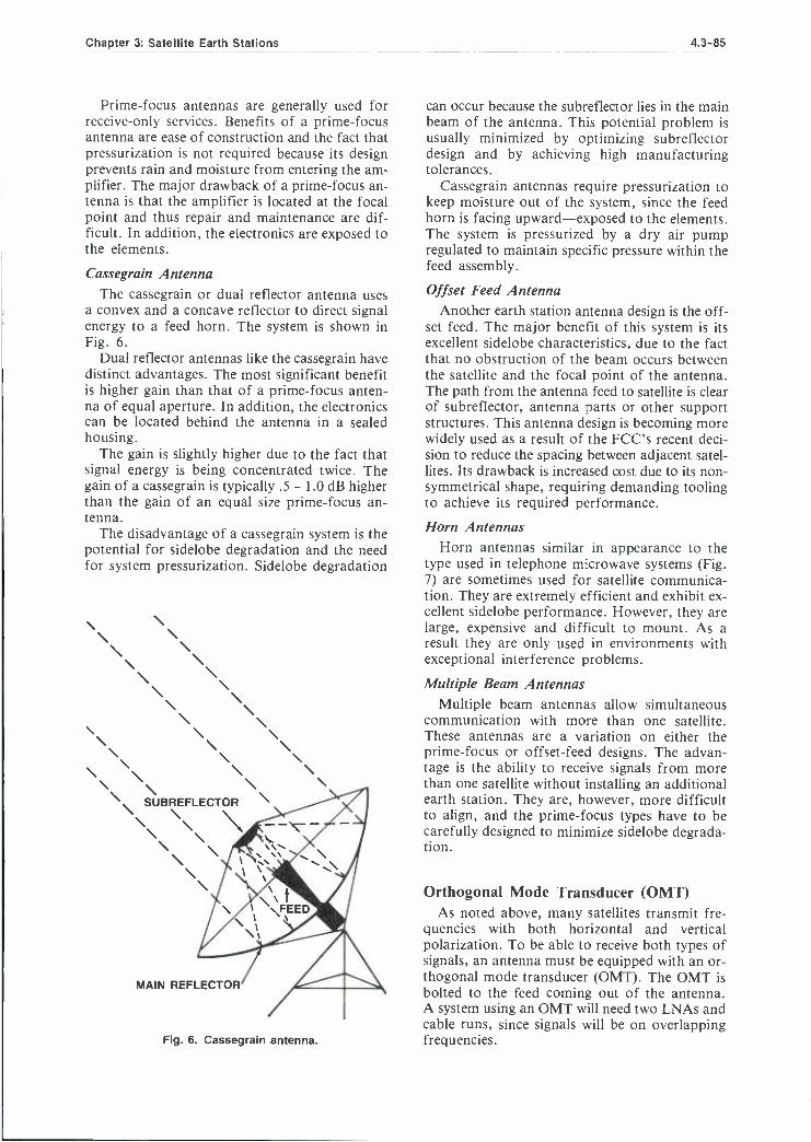
Chapter 3: Satellite Earth Stations 4.3 -85
Prime -focus antennas are generally used for receive -only services. Benefits of a prime -focus antenna are ease of construction and the fact that pressurization is not required because its design prevents rain and moisture from entering the am- plifier. The major drawback of a prime -focus an- tenna is that the amplifier is located at the focal point and thus repair and maintenance are dif- ficult. In addition, the electronics are exposed to the elements.
Cassegrain Antenna The cassegrain or dual reflector antenna uses
a convex and a concave reflector to direct signal energy to a feed horn. The system is shown in Fig. 6.
Dual reflector antennas like the cassegrain have distinct advantages. The most significant benefit is higher gain than that of a prime -focus anten- na of equal aperture. In addition, the electronics can be located behind the antenna in a sealed housing.
The gain is slightly higher due to the fact that signal energy is being concentrated twice. The gain of a cassegrain is typically .5 - 1.0 dB higher than the gain of an equal size prime -focus an- tenna.
The disadvantage of a cassegrain system is the potential for sidelobe degradation and the need for system pressurization. Sidelobe degradation
\ \ \ \ \ SUBREFLECTOR \ \
\ \ \ \ \ \
MAIN REFLECTOR
Fig. 6. Cassegrain antenna.
can occur because the subreflector lies in the main beam of the antenna. This potential problem is usually minimized by optimizing subreflector design and by achieving high manufacturing tolerances.
Cassegrain antennas require pressurization to keep moisture out of the system, since the feed horn is facing upward- exposed to the elements. The system is pressurized by a dry air pump regulated to maintain specific pressure within the feed assembly.
Offset Feed Antenna Another earth station antenna design is the off-
set feed. The major benefit of this system is its excellent sidelobe characteristics, due to the fact that no obstruction of the beam occurs between the satellite and the focal point of the antenna. The path from the antenna feed to satellite is clear of subreflector, antenna parts or other support structures. This antenna design is becoming more widely used as a result of the FCC's recent deci- sion to reduce the spacing between adjacent satel- lites. Its drawback is increased cost due to its non- symmetrical shape, requiring demanding tooling to achieve its required performance.
Horn Antennas Horn antennas similar in appearance to the
type used in telephone microwave systems (Fig. 7) are sometimes used for satellite communica- tion. They are extremely efficient and exhibit ex- cellent sidelobe performance. However, they are large, expensive and difficult to mount. As a result they are only used in environments with exceptional interference problems.
Multiple Beam Antennas Multiple beam antennas allow simultaneous
communication with more than one satellite. These antennas are a variation on either the prime -focus or offset -feed designs. The advan- tage is the ability to receive signals from more than one satellite without installing an additional earth station. They are, however, more difficult to align, and the prime -focus types have to be carefully designed to minimize sidelobe degrada- tion.
Orthogonal Mode Transducer (OMT) As noted above, many satellites transmit fre-
quencies with both horizontal and vertical polarization. To be able to receive both types of signals, an antenna must be equipped with an or- thogonal mode transducer (OMT). The OMT is bolted to the feed coming out of the antenna. A system using an OMT will need two LNAs and cable runs, since signals will be on overlapping frequencies.

4.3 -86 Section 4: Program Transmission Facilities
CONICAL HORN REFLECTOR
ANTENNA
Fig. 7. Conical horn reflector antenna.
Low Noise Amplifier (LNA) The low noise amplifier (LNA) amplifies the
signal at the output of the earth station antenna. The most commonly used LNAs use gallium arsenide field effect transistors (GaAsFETs). Typical noise temperatures for this amplifier range from 75 °K to 120 °K. A thermoelectrical - ly cooled amplifier reduces the noise temperature further, but at significantly higher cost. The selec- tion of an appropriate LNA depends on antenna size and overall system losses.
There is a basic tradeoff between LNA noise temperature and antenna size (that is, gain), ex- pressed by the system figure of merit G /T. Smaller antennas require a cooler LNA for equivalent system performance. A larger anten- na allows use of an LNA with a higher noise tem- perature and lower cost.
The LNA is powered either by dc or ac cur- rent. A dc powered LNA can be supplied power through the output signal cable from the receiver or through a separate cable.
The LNA is a weatherized unit that provides sufficient gain to transport the signal from the antenna to the receiver. The LNA usually has waveguide input to connect the antenna feed as- sembly and a coaxial output.
Low Noise Converter The low noise converter (LNC) combines the
functions of an LNA and a down converter. It is usually located at the antenna which feeds the receiver. The low noise converter changes one channel of the 3.7 to 4.2 GHz frequency to an
intermediate frequency. By downconverting first the LNC allows the use of low loss coaxial cable rather than waveguides to connect the LNC to the satellite receiver. However, local oscillator phase noise is introduced by the LNC, which makes it more difficult to maintain a broadcast quality signal. This along with the higher cost of an LNC means that LNAs tend to be the pre- ferred choice for broadcasters.
SITE SELECTION There are many factors that must be considered
in the selection of a site for a transmit /receive or receive -only earth station. These considerations include:
A clear view of the satellite arc
Future building plans in the area
Interference considerations
Soil conditions Zoning, building codes and related regulatory issues
Connection with ultimate destination of signals
The domestic satellite arc runs from 65 ° to 145 °
west longitude. For all practical purposes, an earth station used for broadcasting should have a clear view of the entire satellite arc, even if it may be receiving signals only from one or a few of the satellites now in use, to be able to make the most of the earth station in the future. No trees, buildings, terrain or other obstacles should obstruct the view. Even minor blockage can sig-

Chapter 3: Satellite Earth Stations 4.3 -87
nificantly reduce or obliterate the very weak sig- nal coming from a satellite.
When selecting the earth station location, fu- ture building plans near the earth station site should be researched and taken into considera- tion.
Rooftop locations are rarely desirable for a satellite earth station. The reduction in atmo- spheric attenuation is negligible and the station is not significantly closer to the satellite. The roof- top antenna faces a far greater likelihood of in- terference from terrestrial microwave systems which use the same 4 GHz and 6 GHz bands. Obviously, it also costs more to survey, plan, get permits for and construct a rooftop earth station.
Perhaps the most important consideration for a site after its unobstructed view of the satellite arc is its shielding from other signal sources. This issue is discussed in detail in the following section.
An additional consideration in site selection is its accessibility for maintenance and repair. It is desirable to have access by standard transporta- tion at all times during the year.
A review of the local planning, zoning, en- vironmental and building requirements should be made early in the evaluation process.
Finally, if a remote site turns out to be the on- ly feasible alternative, consider the availability and reliability of electrical and telephone service from the site.
INTERFERENCE Interference is a significant enough problem for
satellite system operating in the C band to merit separate consideration. The C band is shared be- tween satellite service and common carrier ter- restrial microwave (telephone companies). The FCC requires new transmitters in the band to notify current users within a coordination con- tour defined by FCC rule and provide them with technical data on their proposed operation. The current users make an independent study of in- terference potential and report their objections, if any. The applicant must respond and get the objector's agreement -in writing -that no inter- ference will result or if interference does result, it will be acceptable. After this process, called frequency coordination is complete, the new transmitter can apply for an FCC license.
For a receive -only earth station no prior fre- quency coordination is required. However, the interference potential affects receive stations as well as transmitters. The C band user has the right to license his receive -only earth station and thus the right to be heard when new microwave links are proposed.
The FCC will accept license application for transmit antennas of nine meters or greater for
broadband (video) applications. For narrowband transmission (for instance, SCPC or digital radio), there is no limit on antenna size. Receive stations of any size may be licensed, although antennas smaller than 4.5 meters are only pro- tected to the extent that a 4.5 meter antenna would require.
The 4 GHz band used for signals from satellite to earth is shared primarily with AT &T and the former Bell operating companies. They use horn reflector antennas with very good radiation char- acteristics, and thus only present a problem when they are nearby or if the receive station is direct- ly under a path. Unfortunately, that happens fair- ly often, due to the number of paths involved.
The situation is more complicated for the transmitting stations at 6 GHz. Non -Bell com- mon carriers and earth stations on this band generally use less discriminating antennas that allow more gain off the main beam of the anten- na. In addition, there are more paths and the margin of protection for the terrestrial system is 10 -16 dB greater than for an earth station.
Fundamental to an interference analysis is knowledge of how new and existing antennas emit and accept radiation off their "main beam." This information is available from the antenna manu- facturer or standard FCC specifications are sub- stituted. For any computation involving satellite earth stations, the analysis must take into account the fact that the antenna will be rotated to view a number of satellites and the fact that, unlike a terrestrial system, the earth station main beam usually points well above the horizon. The basic antenna gain chart in Part 25 of the FCC Rules is used as a basis for developing a horizon gain curve taking these factors into account.
Interference propagates along great circle paths. On unobstructed paths, free space loss is the primary factor reducing the interference level. If the path is blocked, diffraction or tropospheric scatter means that some interfering energy will nevertheless reach the antenna. The basic equa- tion for calculating interference level is:
Pr= Pt+Gt- L+Gr
Where:
Pr = received signal power (dBw) Pt = transmitted power (dBw) Gt = gain of the transmitter in the direc-
tion of the earth station (dBi) L = basic transmission loss (free space loss
or loss from diffraction and tropo- spheric scatter effects) (dB)
Gr = gain of the earth station antenna in the direction of the transmitter (dBi)

4.3 -88 Section 4: Program Transmission Facilities
This same equation determines interference caused by a transmitting earth station, with the role of transmitter and earth station reversed.
FCC rules establish the criteria that determine which microwave stations must be included in fre- quency coordination for a transmitting earth sta- tion. Similar criteria can be used to identify potential interference sources for a receive -only station.
Licensing for a transmitting or receiving earth station involves three steps. First, before coor- dination begins, the broadcaster conducts his own study of the interference environment. This can most easily be done using a computer study from one of the frequency coordination services with a data base of existing and approved microwave and earth station licenses. This study will include some consideration of terrain and may be augmented by field testing.
Second, once the user has satisfied himself that the station will operate without interference, he (or his frequency coordinator) issues the coordina- tion notice. Then he responds to the objections of existing users.
Finally, once all parties agree on interference considerations, an FCC license application can be filed.
Often more than just an office study is needed to clear a proposed site, because many of the figures used in calculating expected interference are conservative estimates and because topographic map data usually underestimates isolation provided by buildings and trees. A field test will often clear a case showing marginal in- terference. For receive -only stations, the field test directly evaluates interfering signals. For a trans- mitting station, the test measures the isolation be- tween the site and existing transmitters.
Field measurements are taken with a test anten- na and a spectrum analyzer. The test antenna is scanned 360 ° in both vertical and horizontal polarizations, while the spectrum analyzer is set to display the full 500 MHz of either the 4 GHz or 6 GHz bands. Typically a daytime and a night- time test is made and statistical models are used to estimate the results in the worst season and under the worst short -term conditions.
There are a number of things that can be done to prevent interference. Natural shielding remains the best and cheapest solution. If there is a choice between a hilltop site and a valley site with a view of the satellite arc, choose the valley. Trees can also reduce interference, but remember to take into account the loss of leaves.
Diffraction fences of hardware cloth, expand- ed metal or chain link fence with metal strips in- serted in the mesh can also be used to shield. Pre- fab shielding material is also available for this purpose. It is often difficult to calculate in ad- vance the precise effect of diffraction fences close
to the antenna, since the fence must be considered as part of the antenna itself.
Pit shielding (building earthen mounds around the earth station) can provide more than 25 dB of additional isolation. Drainage should be pro- vided if the pit completely surrounds the antenna.
A higher -performance (more directive) anten- na can sometimes solve interference problems.
Because of the differences in channeling be- tween terrestrial microwave and satellite systems, a good notch filter 10 MHz above or below the center of the desired receive frequency will sometimes resolve interference. This approach is only available for receive -only stations and only applies to interference from FDM /FM sources. It will not resolve interference from digital, single - sideband or FM video.
Finally, there is the option of choosing a com- pletely different location for the earth station.
Early in the planning stages for an earth sta- tion, it is possible to obtain an interference in- tensity map. This shows expected worst -case in- terference levels at a number of equally- spaced locations within a large target area. This map can be used as a guide in finding a location with the right topography, zoning and price. The chosen site will still require detailed interference analysis, but the potential for unpleasant surprises is sub- stantially reduced.
FCC LICENSE The FCC requires licensing of transmitting
earth stations and permits licensing of receive - only earth stations. It is desirable for a broad- caster to license a receive -only station, since licensing protects the station from future in- terference from domestic microwave systems.
The receive -only application is relatively sim- ple. It is a narrative (there is no standard form) with the following information:
1 . The nature of the proposed service.
2. A statement of public interest.
3. The name of a person to receive corre- spondence (usually includes a technical con- tact and counsel).
4. The applicant's technical qualifications.
5. A paragraph identifying that the application is a "minor" action for environmental con- siderations. Generally, the action is minor if the antenna dish is less than 30 feet in diameter and is not located in certain specific areas (e.g. historic districts, scenic areas, floodplains and some others listed in 47 CFR 1.1305(a)(6)).
6. Description of the site (plot plan) and its availability. This should include the eleva-
Chapter 3: Satellite Earth Stations 4.3 -89
tion of the antenna base above sea level and the maximum antenna height above the base.
7. A functional block diagram of the system.
8. Description of the antenna mounting and range.
9. A statement of compliance with the require- ments for antenna sidelobe performance.
10. A statement of FAA clearance, if required (the same rules apply as for any antenna).
11. The report of frequency coordination and interference analysis.
12. A technical showing that the antenna meets the performance criteria for a 4.5 meter an- tenna, if the antenna is less than 4.5 meters.
13. A completed FCC Form 403.
14. A technical summary of the proposed sta- tion including a description of the equipment to be used, major structures, the type of communication being received, the space segment being accessed, frequencies and polarities received, satellites and trans- ponders being used.
15. A statement that the applicant will only re- ceive program material for which it has ob- tained rights.
16. The applicant's certification.
17. The technical certification by a technically qualified person that the engineering data is complete and accurate.
These same items are required for transmitting stations, although naturally some of the items will be more involved (such as frequency coordina- tion and technical description of the system). There are a few additional requirements for trans- mitting stations:
1. A completed FCC Form 430 (legal and financial qualification). This form is re- quired if common carrier status is sought.
2. A statement of compliance with regulations for the protection of employees and the gen- eral public against excessive radiation.
3. A statement of compliance with FCC regula- tions regarding quiet zones.
INSTALLATION This section consists of a checklist of considera-
tions in constructing a satellite earth station.
Foundation In selecting the precise location for the anten-
na, it is important to choose a level site, well drained and free from underground obstructions
that might interfere with foundation construction. The foundation for the antenna will be substan- tial to maintain the pointing angle of the anten- na despite substantial wind loading and possible ice loading. An evaluation of soil type and frost penetration is necessary to establish the founda- tion required.
There are two common types of foundation. In the mat footing, the load is borne by a single, large reinforced concrete mat. The alternative, a drilled pier footing, requires much less concrete and are more cost -effective if soil conditions per- mit their use. Further economies can be achieved with earth anchors supplementing concrete piers. Pier kits are available for smaller earth stations.
The mat foundation may be required if the ground is too rocky or the soil too loose for drill- ing holes for piers. Sometimes it is too expensive to transport pier drilling equipment to the pro- posed site. In some areas small contractors may be able to build a mat foundation at less cost.
As mentioned above, rooftop locations are not recommended for earth stations. If a rooftop location is required, it is necessary to construct a load frame to connect the antenna mount to the building columns. As height increases, ex- pected wind load increases and the design of the antenna mount needs to be adjusted accordingly.
Note that a professional engineer may be re- quired to approve a foundation design in some states.
Finally, before the foundation is poured, be sure that provision has been made for supplying ac power and RF interfacing, if it will pass through the foundation.
Mounting There are a number of systems for mounting
and pointing earth stations, some with two mov- ing axes, some with one. As might be expected, the one -axis systems sacrifice some accuracy in the interest of simplicity.
The two -axis systems are elevation -over- azimuth (with one axis of rotation perpendicular to the plane of the horizon), X -Y (with one axis parallel to the ground) and polar (with one axis parallel to the earth's axis of rotation). Elevation - over- azimuth is an extremely flexible system, and initial mounting is not critical. It is more com- plicated than the other systems. X -Y requires that careful attention be given to the initial heading angle of the antenna.
The polar system has the advantage that it can maintain pointing at any point in the sky simply by rotating about its vertical axis. For this reason, the polar mount is the basis for the single -axis mounting systems. In a simple single -axis system, the vertical mount is exactly parallel to the earth's axis of rotation. In a declination- corrected polar mount system, a slight correction is made to ac-

4.3 -90 Section 4: Program Transmission Facilities
count for the fact that the antenna is not in the same plane as the satellite arc (that is, the plane of the equator). In most parts of the continental U.S., a declination- corrected polar mount anten- na can be made to point to any satellite between 70° and 135 ° west longitude with negligible error.
Heading Accurate heading of the antenna center line is
often essential for finding the desired satellites. With some mounting systems, an inaccurate foun- dation heading may require reconstruction, and the foundation contractor should be made aware of the importance of maintaining a surveyed heading. A competent surveyor can establish the proper heading by reference to known survey lines, by pole star observation or by compass. The last should take into account magnetic declina- tion from true north and, in any case, should not be used near large metal structures or strong elec- trical fields.
Shelters For receive -only earth stations in remote loca-
tions, the necessary electronics can often be located in a simple equipment shelter (8 ' x 8 '). Since the equipment generally does not generate a large amount of heat, it may be possible to avoid air conditioning.
Shelter requirements become significant for a transmitting earth station. Each HPA is about 2 ' wide, 3 ' deep and 7 ' high, and a typical sta- tion will have redundant HPAs for reliability. Control equipment will occupy two standard 19" racks. Sufficient space is needed for waveguides and cable runs. A 10' x 18' shelter is probably the minimum for accommodating the necessary equipment.
Any shelter should be as close to the earth sta- tion as possible to avoid long cable runs. If long runs cannot be avoided, additional amplifiers will be needed along the run.
Power Power requirements for a receive -only station
are modest, probably less than 1 kW for the LNAs, receiver and control equipment. Motorized antenna positioning would require additional power. For transmitting stations, HPAs demand large amounts of power, perhaps 12 kW of three - phase power for a 3 kW video amplifier. A hot backup HPA requires a doubling of the load. Antenna deicing represents the other major power requirement, with 3 kW for feed and subreflec- tor deicing (sufficient in milder areas) up to 51 kW for full reflector deicing. Air conditioning is an additional power consumer.
Two kinds of backup power should be con- sidered. Short outages can be bridged with an uninterruptible power system (UPS), a battery-
based system. It is impractical for a UPS to pro- tect anything but the electronics of the system. An engine and generator is needed for longer outages. This system should be sufficient to operate the entire system, with provision for enough fuel to maintain operation when condi- tions may hamper refueling.
Pressurization A pressurization unit must be installed to keep
moisture out of certain earth station antennas, notably cassegrains. Pressure may also be re- quired for air dielectric cabling.
OPERATION Operating an earth station antenna is above all
a matter of correct pointing. The process should be one of pointing to the correct azimuth and elevation of the desired satellite and then fine tun- ing, first with the meters of the satellite receiver and then with a video monitor.
For a transmitting station, a scenario for start- ing transmission might follow these lines:
1. Position antenna on satellite (can use receivers to insure accurate pointing).
2. Check null on adjacent transponders to verify polarization angle.
3. Tune exciter, HPA and Receiver to the trans- ponder frequency.
4. Check power levels with a dummy load. 5. Call the satellite technical operations center to
initiate transmission.
6. Transmit low -power CW to check polarization.
7. Operations center clears full -power transmis- sion.
8. Increase power.
9. Add modulation (test tone). 10. Check for interference on adjacent transpon-
ders.
11. Add source.
12. At the end of transmission, call operations cen- ter to inform them.
MAINTENANCE Maintenance will usually be specified by equip-
ment manufacturers. There are few moving parts or sensitive equipment with a receive -only station, so maintenance will not be a major item. Anten- na bolts should be checked and tightened periodically. Waveguides should be checked for

Chapter 3: Satellite Earth Stations 4.3 -91
leaks and kinks. Antenna motors should be checked and lubricated as required. Weekly in- spection should identify impending problems.
For a transmitting station, HPAs require dai- ly inspection. The klystron tube in an HPA will
need to be rebuilt every two to three years, so that a redundant system with two HPAs will re- quire 3 klystrons, two operating and one in repair.
A rule of thumb for maintenance is 3% to 5% of system cost per year.

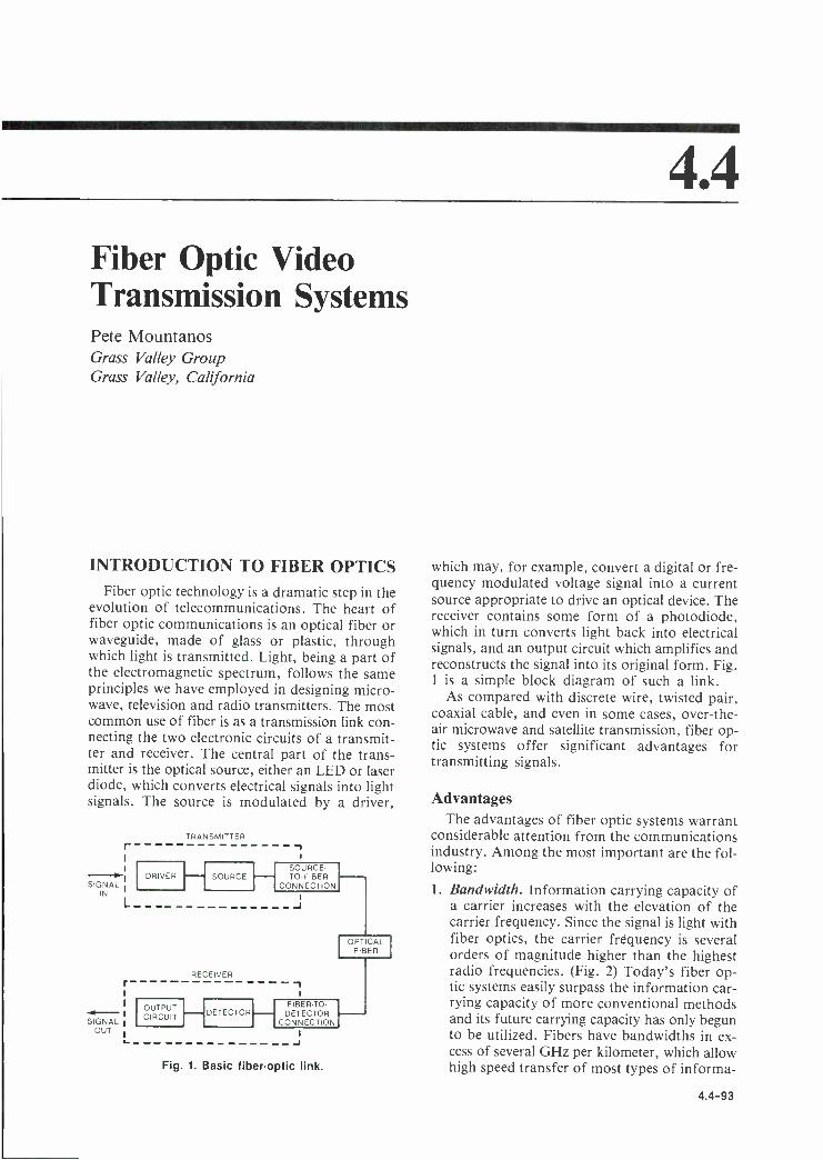
4.4
Fiber Optic Video Transmission Systems Pete Mountanos Grass Valley Group Grass Valley, California
INTRODUCTION TO FIBER OPTICS Fiber optic technology is a dramatic step in the
evolution of telecommunications. The heart of fiber optic communications is an optical fiber or waveguide, made of glass or plastic, through which light is transmitted. Light, being a part of the electromagnetic spectrum, follows the same principles we have employed in designing micro- wave, television and radio transmitters. The most common use of fiber is as a transmission link con- necting the two electronic circuits of a transmit- ter and receiver. The central part of the trans- mitter is the optical source, either an LED or laser diode, which converts electrical signals into light signals. The source is modulated by a driver,
r
SIGNAL IN
L
r
i
SIGNAL OUT
TRANSMITTER
DRIVER HSOURCE HSOURCE- TO-FIBER
CONNECTION
-J
RECEIVER
OUTPUT CIRCUIT DETECTOR
IOPT CAL FIBER
FIBER-TO- DETECTOR
CONNECTION,
J Fig. 1. Basic fiber -optic link.
which may, for example, convert a digital or fre- quency modulated voltage signal into a current source appropriate to drive an optical device. The receiver contains some form of a photodiode, which in turn converts light back into electrical signals, and an output circuit which amplifies and reconstructs the signal into its original form. Fig. 1 is a simple block diagram of such a link.
As compared with discrete wire, twisted pair, coaxial cable, and even in some cases, over -the- air microwave and satellite transmission, fiber op- tic systems offer significant advantages for transmitting signals.
Advantages The advantages of fiber optic systems warrant
considerable attention from the communications industry. Among the most important are the fol- lowing:
1. Bandwidth. Information carrying capacity of a carrier increases with the elevation of the carrier frequency. Since the signal is light with fiber optics, the carrier frequency is several orders of magnitude higher than the highest radio frequencies. (Fig. 2) Today's fiber op- tic systems easily surpass the information car- rying capacity of more conventional methods and its future carrying capacity has only begun to be utilized. Fibers have bandwidths in ex- cess of several GHz per kilometer, which allow high speed transfer of most types of informa-
4.4 -93

4.4 -94 Section 4: Program Transmission Facilities
FREQUENCY (Hz)
1022- -4-- Cosmic Rays
-.- -Gamma Rays
-4- X -rays
Ultraviolet Light
WAVELENGTH (nm)
Ultra- violet
400
1021--
1020-- 10i9- 1018 - 10" Violet
455
- e-- 10'
Blue 490 1015_
10'"-- Green f-- Visible Light 1013--
- _. _-4--
550 Yellow
580 f Infrared
Light
-4- Radar
Television and FM Radio
Shortwave Radio
(1 THz) 1012- Orange 620
Red 750
10"- 101°
GHz) Infrared 800
850
SPEED OF LIGHT
(1 109-.. 10° - 10'
MHz) 108 Radio -4- AM Radio Frequencies
-4- Sound
WAVELENGTH =
Subsonic
(1 - 10° -- 10° -
KHz) (1 10' - 102 --
FREQUENCY 10 - o
-.4-
Fig. 2. Electromagnetic spectrum.
tion. With multiplexing, many signals can be sent over a single fiber. For example, the phone industry now transmits thousands of voice channels simultaneously over a single optical waveguide.
2. Low Loss. Fibers provide substantially lower attenuation than copper wires and require no equalization. In premium cables attenuation can be below .5 dB /km for certain wave- lengths.
3. Electrical Isolation. Since the fiber cable is essentially dielectric material it is inherently isolated electrically. There is no spark hazard, and no risk of EMI emmissions. Fiber cable is a natural in hazardous environments, and its electrical isolation precludes ground loop problems. Fiber optic systems are immune to outside electrical noise as well.
4. Size and Weight. In general, the optical wave - guide is the size of a human hair. As a result an equivalent copper cable is always much larger, stiffer and heavier than an equivalent fiber cable. Thus, installation costs, ducting, handling costs and the like are typically much
lower for a fiber installation than for a similar coaxial system. This factor alone accounts for much of the rapid acceptance of fiber.
Disadvantages Optical fiber as a transmission medium does
have disadvantages, some of which are strictly due to the relative infancy of the technology. A major disadvantage is lack of fiber optic stan- dards from industry organizations such as EIA. This lack of standards in both specifications and testing procedures makes comparison of various manufacturers' products difficult. It is expected that these problems will be addressed in the near future. Another drawback, most significant to the broadcast industry, is the difficulty of adapting fiber optics to existing systems. Most intercon- nections rely on linear analog amplifiers such as distribution amplifiers. Fiber optics is not suited for such implementation as it is preferable to operate in a serial pulsed fashion. As the cost of fiber optic components declines, and the use of digital components in television increases, the technology will become increasingly appropriate.

Chapter 4: Fiber Optic Video Transmission Systems 4.4 -95
Economics The economics of using fiber optic systems is
a complex discussion. Direct comparisons be- tween copper based, microwave or satellite based systems are difficult and open to debate. Each evaluation must be based on the user's needs. It is clear that widespread application of any tech- nology depends upon providing superior perfor- mance at a lower cost to competing technologies. That fiber optics can meet such a criteria has been established by the telephony industry. As is the case with most new technologies, costs are rapidly dropping while more mature technologies con- tinue to increase. As a result, fiber optics becomes more attractive every day.
LIGHT AND FIBER CHARACTERISTICS
Light is similar to radio waves, x -rays, and gamma rays in that it is a part of the elec- tromagnetic spectrum. In general the frequencies of light used in fiber optic transmission are in the region of 300 -400 terrahertz (10xE14), or several orders of magnitude higher on the elec- tromagnetic spectrum than the highest frequen- cy radio waves. Light waves are more generally described in terms of wavelength rather than fre- quency (Fig. 2). The region extending from 800 -1600 nanometers is of greatest interest because today's fibers propagate these wave- lengths most efficiently.
What we refer to as "the speed of light" (300,000 km /sec) is the velocity of any electro- magnetic energy in free space or a vacuum. Light travels slower in all other media, and different wavelengths travel at different speeds in any single medium. When an electromagnetic wave crosses a boundary from one medium to the next it changes speed which results in a change of path called refraction.
The index of refraction, n. is a dimensionless number expressing the ratio of the velocity of
LIGHT PATH FRESNEL
REFLECTION
0= CRITICAL NORMAL ANGLE
n
n, n,
light in free space, c. to its velocity in a specific medium. Thus:
n = c/v
Refraction of a ray of light as it passes from one material to the next depends on the refrac- tive index of the material. When discussing refrac- tion three terms are used. The normal is the line perpendicular to the interface of the materials. The angle of incidence is the angle between the incoming ray and normal. The angle of refrac- tion is the angle between normal and the refracted ray.
When light passes from a high index of refrac- tion medium to a lower one the light is refracted toward the normal. Fig. 3 shows that as the angle of incidence increases, the angle of refraction ap- proaches 90 degrees with normal. This is called the critical angle. If the angle is increased past the critical the light is totally internally reflected.
Optical Fibers A basic optical fiber consists of two concen-
tric layers. The inner layer, the core, has a refrac- tive index higher than the outer layer, the clad- ding. Light injected into the core and hitting the boundary at an angle greater than critical is reflected into the core. Light striking the inter- face at less than the critical angle is passed into the cladding and lost. This total internal reflec- tion forms the basis for light propagation in op- tical fibers. The exact characteristics of light pro- pagation depend on fiber size, construction and composition. Maxwell's equations show that light does not travel randomly through a fiber; but rather that it is channeled into modes. A mode is a possible path through a fiber.
Types of Fibers There are many ways to classify fibers, however
the most informative are by refractive index pro- file and number of modes supported. The two
= 90
ANGLE OF _ ANGLE OF INCIDENCE REFLECTION
Fig. 3. When the refractive index. of the first medium (n.) is greater than that of the second, (n.) light is refracted away from the normal. If the angle
of incidence is greater than the critical. the light is totally reflected.

4.4 -96 Section 4: Program Transmission Facilities
main types of index profiles are step and graded. In a step index fiber, the core has a uniform in- dex with a sharp change at the boundary of the cladding. In graded index fiber, the core's index is not uniform; it is highest at the center and decreases until it matches the cladding. There is no sharp break. Fig. 4 shows the paths and pro- pagation characteristics of such fibers.
Multimode, Step Index A multimode step index fiber typically has a
core diameter in the 500 -1000 micron range. The large core permits many modes of propagation. Since light will reflect differently for different modes some rays follow longer paths than others. The lowest order mode travels down the center while higher modes strike the core -cladding in- terface at angles near the critical angle and as a result, follow longer paths through the fiber. As a result, a narrow pulse of light spreads out as it travels through this type of fiber. This "spreading" is called modal dispersion.
Single or Mono Mode, Step Index A way to limit modal dispersion is to make the
fiber core sufficiently small to insure the fiber propagates only one mode efficiently. A single mode fiber has a core diameter small enough that the fiber propagates only one mode, efficiently. A single mode fiber has a core diameter of the
INPUT OUTPUT PULSE PULSE
J. /
i
order of 5 -10 microns. This is of the order of 1 /6th the diameter of a human hair. Its small size makes it very difficult to work with, however it is very efficient and suitable for high speed, long distance transmission.
Multimode Graded Index A graded index fiber also limits modal disper-
sion. Its core is essentially a series of concentric rings, each with a lower refractive index. Since light travels faster in a lower index medium, light farther out from the axis travel faster. Since high order modes have a faster average velocity than low order modes, all modes tend to arrive at a point at nearly the same time. Rays of light are not sharply reflected by the core -cladding inter - face, they are refracted successively by different layers in the core.
Dispersion Dispersion relates to the spreading of a light
pulse as it travels down a fiber. A pulse measured at the output will be wider than it was at the in- put. This limits a fiber's bandwidth or informa- tion carrying capacity. Pulse rates must be slow enough that dispersion will not cause adjacent pulses to overlap. Consider the pulse shown in Fig. 5. Two trains of pulses, one faster than the other are injected into the same fiber. In both cases, the pulses are spread by dispersion. For
DISPERSION REFRACTIVE HIGH -ORDER INDEX MODE PROFILE
MULTIMODE STEP INDEX LOW -ORDER MODE
---7nz n,
SINGLE -MODE STEP INDEX
DISPERSION --
MULTIMODE GRADED INDEX
Fig. 4. The core size and refractive index determine the light propagation characteristics of the fiber.

a
Chapter 4: Fiber Optic Video Transmission Systems 4.4 -97
v_
---á 6---- EACH PULSE APPARENT
y PULSES MERGED
Fig. 5. Dispersion limits signal frequency.
the slower train, the interval between pulses is
sufficient to allow each pulse to be distinguished. In the faster train, however, the interval is so short that individual pulses merge into one long indistinguishable pulse. Dispersion, which can be related to pulse rise and fall times as in copper cable, therefore is the limiting factor in deter- mining a fiber's bandwidth.
There are basically two types of dispersion: modal, resulting from differing path lengths already discussed; and material, arising from dif- fering velocities of different wavelengths in the signal. In a single mode fiber there is no modal dispersion, only material dispersion limits its capacity for carrying information.
Material Dispersion is generally limited by either operating at lower frequencies, or using very narrow optical spectrum devices such as lasers.
Attenuation or Loss Attenuation is loss of power. During transit
some of the light is absorbed into the fiber or scattered by impurities. Attenuation for a fiber is usually specified in decibels per kilometer or dB /km. For commercially available fibers, at- tenuation ranges from around .5 dB /km for premium fibers to 100 dB /km for large core plastic fibers. It is important to remember that since we are measuring optical power, a 3 db loss represents 'A rather than the 6 dB we have be- come used to in dealing with voltages.
Fiber attenuation is closely related to light wavelength. Most fibers have a medium loss region in the 800 -900 nm range (3 -5 dB /km), a low loss region in the 1150 -1350 nm range (.6 -1.5 dB /km), and a very low loss region (less than .5
dB /km) in the 1550 nm area. As a result best per- formance is achieved by careful balancing of fiber, device and distance requirements.
OPTICAL DEVICE CHARACTERISTICS
Sources An optical source is generally either a light
emitting diode (LED) or an injection laser diode. The LED is an incoherent source, which when
compared with a laser, provides less power and operates at slower speeds, but also costs con- siderably less. It is however, quite suitable for most applications requiring transmission less than 10 km and speeds less than 100 Mbits per second. A laser requires more electronics to operate, is
more powerful, and costs more, however it can be used to transmit distances over 100 km before amplifiers are required. In general, an optical source must be evaluated to insure its speed is suitable to the bandwidth required, and that it provides enough optical power at a wavelength suitable to meet the distance requirement. Another important consideration is the fact that optical devices do not turn on with the linear characteristics we are accustomed to with elec- trical devices. Fig. 6 and Fig. 7 illustrate examples of characteristics for lasers and LED's. As a result, modulation techniques that rely on the linearity of the device are generally not suitable for fiber optic applications.
Detectors A detector performs a complimentary function
to the source: it converts incident optical energy back to electrical energy. Common detectors used in fiber optics are semiconductor photodiodes, including PIN and avalanche photodiodes.
The performance of a fiber optic system is generally limited by dispersion or attenuation. When a link is limited by attenuation distance, the detector must respond to weak incoming sig- nals and its sensitivity will determine link per- formance.
In an ideal PIN diode, each incident photon creates an electron -hole pair in the semiconduc- tor lattice. This in turn sets one electron flowing in the external circuit. If the received light is
weak, the generated current may not be strong enough to overcome noise inherent in the diode and receiver circuit. In such cases, it is desireable to increase the detector output before amplifica- tion by the receiver. Such gain is inherent in an avalanche photo diode or APD. A reverse bias provides several electron volts of energy increase to each liberated electron, providing inherent amplification of the received signal. Once again, such amplification is not linear with received levels.

4.4 -98
0
Section 4: Program Transmission Facilities
I
LAS ER
LED
0 20 40 60 80 100 120 140 160 180
D.C. LASER DRIVE CURRENT (MA)
0 2 .4 .6 .8 1 1.2 1.4 1.6 1.8
PIN CURRENT (MA)
Fig. 6. Semiconductor laser turn -on characteristics.
VIDEO AND AUDIO TRANSMISSION TECHNIQUES
Modulation Techniques In general there are three basic ways to
modulate information onto an optical carrier. These are intensity modulation (light amplitude carries the information), frequency modulation (pulse speeds directly correspond to input signal levels), and digital pulse code modulation.
Intensity Modulation Intensity Modulation (referred to as IM or AM)
is the simplest form of modulation. Here an in- coming signal such as video is used to directly drive an optical device. Thus, maximum ampli- tude of video being "white ", would result in the most output light and bottom of sync the least. Unfortunately, as shown in Figs. 6 and 7, op- tical devices do not turn on in a linear fashion. As a result, linear distortions are introduced to the video signal when such modulation techniques are implemented. In addition, the signal -to -noise
MODULATE IN THIS REGION FOR BEST LINEARITY /
i MODULATE IN THIS REGION FOR BEST
SMR
BIAS CURRENT
Fig. 7. Typical LED characteristics.
ratio of the signal is directly correlated to the op- tical power. As a result, attenuation in a system lowers signal to noise directly. Further, since most optical devices do not completely "turn off" (par- ticularly lasers) there is always an optical noise floor present. For broadcast applications (EIA RS- 250 -B) such systems are not widely used.

Chapter 4: Fiber Optic Video Transmission Systems 4.4 -99
Frequency Modulation Frequency modulation devices are often used
to help overcome the limitations of optical devices. In general, an FM approach is more com- plicated and costly but removes the problems of signal quality from the optical domain to the elec- trical domain. Here an input signal (video or audio) is frequency modulated prior to driving an optical device. All problems related to required SNR or linearity are solved by proper design of the frequency modulator. The desired output be- ing a square pulse train where the input signal information is carried in the time domain as pulse spacing. Audio information is generally contained as FM subcarriers added to the video; then the entire signal is remodulated to avoid non lineari- ties in the devices.
PCM or Digital As mentioned earlier, fiber optics is a
technology intended to be operated in a pulsed mode, thus it is particularly suited to FM and digital approaches. In telephony applications, the relatively narrow bandwidth of a single voice channel can be digitized and multiplexed with thousands of other similar channels. Video on the other hand, is a much higher bandwidth signal and results in very high bit rates. In evaluating digital systems a user must keep in mind analog performance requirements. As a result, digital systems are generally evaluated end to end on the basis of the specific application. Two major fac- tors affect digital systems performance: sampling rate and number of bits per sample. The Society of Motion Picture and Television Engineers (SMPTE) has done a very thorough job in cor- relating bits per sample (quantizing error) to equi- valent signal to noise ratio. It is perhaps, worth- while to provide a quick review.
In general, it has been shown that 8 -bit sam- pling can provide excellent television pictures. This will generally result in bit rates (depending on sampling frequency) of up to 115 Mbits. How- ever, this results in an equivalent signal -to -noise ratio of 56 dB. In general, most analog systems have allocations of performance to various por- tions of transmission that can require up to 67 db SNR. Unless the user can insure an entire digital transmission, higher sampling rates should be used. As a guide (again based on SMPTE digital publications), 9 bit sampling systems should be used where 60 dB SNR is required and 10 bit systems where 67 dB SNR is required. Such systems result in bit rates in excess of 150 Mbits per second.
Performance Requirements In general, fiber optic transmission require-
ments must continue to meet the needs of exist-
ing transmission parameters. The EIA RS -250 -B standard has served the industry well and con- tinues to be the bench mark by which transmis- sion systems are measured. It is a very compre- hensive document but in general requires short haul systems (most fiber optic systems today) to deliver 67 DB SNR with 20/o diff. gain and .5 degrees differential phase error. In applications for teleconferencing and CATV obviously lower specifications apply and cost -effective solutions exist for virtually all performance requirements.
Multiple Video Transmission Because of the large information carrying
capacity of fiber optic systems, they are frequent- ly asked to send multiple video signals over a single optical fiber. Where required, there are several methods for accomplishing this. These are Wavelength Division Multiplexing (putting dif- ferent wavelengths of light onto a single fiber), Frequency Division Multiplexing (putting multi- ple FM subcarriers through a single optical device), and Digital Multiplexing.
Wavelength Division Multiplexing This multiplexing technique is primarily used
to reduce the number of optical fibers required to meet a specific transmission requirement. Basically it requires two or more complete fiber optic transmission systems operating at different optical wavelengths. Utilizing a passive optical multiplexer (basically a prism) multiple optical wavelengths may be placed onto an optical fiber and then removed. Similar techniques can be used to accomplish bidirectional transmission. Several considerations are important in designing such systems.
First, adequate separation (measured in dB of each optical channel is required. Optical crosstalk between channels results in lowering the effec-
840mm VIDEO
TRANSMITTER FOL OPTICAL FOL
MUX 1300mm FOL VIDEO
TRANSMITTER
840mm VIDEO
RECEIVER FOL OPTICAL
DEMULTIPLEXER 1300mm j70r_ VIDEO
RECEIVER
Fig. 8. Typical WDM configuration (FOL = fiber-optic link).

4.4 -100 Section 4: Program Transmission Facilities
tive SNR of the link. Secondly, passive devices result in some optical attenuation when used (1 -5 dB per device). As a result, effective transmis- sion distances must be reduced when attempting to use WDM techniques. Lastly, most optical devices change output wavelength over tempera- ture and the band pass of such WDM devices must be wide enough to accommodate the range. In general, fiber costs have dropped sufficiently that WDM is only cost effective when used to add capacity to existing installations. Further- more, since optical separations are relatively poor, WDM techniques are only appropriate for FM and digital systems whose carrier -to -noise require- ments are equivalent to or less than the WDM components.
Digital Multiplexing As mentioned earlier, digital transmission rates
for video are very high, particularly with regard to short haul requirements in an analog domain. However, even rates of 180 Mbits (243 for serial digital components) are less than current tele- phony rates. Serial transmission of 565 Mbits are now commonplace with demonstrations in the gigabit range occuring by numerous manufac- turers. As a result such high speed transmission offers the promise of low cost high bandwidth channels. As these systems are proliferated it is increasingly obvious that multiple high quality video transmission will be most cost effective over fiber optics systems. In general, multiplexing ap- plies equally to ancillary signals. Audio and data channels are similarly multiplexed together or with video using one or more of the above mul- tiplexing techniques.
INSTALLATION CONSIDERATIONS Installation of fiber optic systems is rapidly in-
creasing. System design of each system requires numerous considerations, the following represents a guide to implementing a system.
Performance Requirements First, the system engineer must determine what
end to end performance requirements are need- ed. For video this can range from a very high performance entrance link to a low performance security camera. Determining performance re- quirements first can expedite equipment evalua- tion and insure the most cost -effective solution.
Once system performance of a link is deter- mined, optical loss budgeting must occur. This is governed by the distance required and the manufacturer's specifications. In general, fiber optic systems specify an optical loss budget at a
given wavelength. Subtracting from this number connector losses, splice losses, fiber losses, and future margins for additional splices and /or WDM components, will determine whether a par- ticular system is acceptable and whether repeaters are required.
Optical loss affects the performance of a fiber optic system. Thus, it is worthwhile to minimize these wherever possible. In general, the optical loss of a link should always be measured to in- sure it meets calculations. There are basically two methods. First, an instrument called an Optical Time Domain Reflectometer (OTDR) is frequent- ly used to measure attenuation or look for breaks in the fiber. It operates on the principle of send- ing a pulse of light and evaluating back scattered or reflected light in the time domain. This instru- ment provides a graphical representation of the fiber as a function of distance. It can literally pin- point a break in a fiber to approximately a meter even over 10's of kilometers.
A simpler method is to use a simple optical meter and the system being installed. First, the user measures output power of the transmitter or launch power. This should be done with a patch cord to account for the first connector in- terface. Then, at the end of the fiber, received power is measured to insure it meets expectations. Once this is accomplished, the fiber optic system installation can be completed.
Frequency Division Multiplexing This technique involves multiple FM modula-
tors operating at different carrier frequencies and then summation of the signals. This is a widely used technique in coaxial cable distribution. Un- fortunately, in optical systems the non -linearity of the optical devices results in large intermodula- tion distortions. As a result, wide spacing of car- riers has been required in systems built to date. Further, insufficient experience has been gained regarding changes in device characteristcs with time that could result in long term increases in intermodulation distortions. This technique re- quires operation of the optical devices in an in- tensity modulation mode, which as discussed earlier, is not a desired application in fiber op- tics. This however, may turn out to be suitable for lower quality transmission requirements in the future such as CATV or teleconferencing.
Cable Specifications In general, specifying cable for transmission ap-
plications is relatively easy. Step index fibers cost the same as higher performance multimode or single mode fibers but do not offer bandwidth. As a result, single mode or multimode fibers are

Chapter 4: Fiber Optic Video Transmission Systems 4.4 -101
chosen. They are comparably priced and the selec- tion criteria is based on other factors. Because multimode fibers are larger in core diameter they are easier to splice and connectorize. However, they have higher attenuation and lower band- width. As a result, in very long distance transmis- sion (greater than approximately 25 Km), single mode is generally used. In shorter distances, (with the exception of telephony which is such a large user) standardization and large bandwidths lends itself to single mode) multimode cables are gen- erally selected. In choosing a cable, numerous fac- tors should be considered. 1. Attenuation. This will determine distance. It
is specified in terms of dB /km. Thus if a cable has a specified attenuation of 3 dB /km, 4 kilo- meters will attenuate 12 dB of light. Remember attenuation is a function of wavelength. Short wavelength (800 -900 nm) is used for short distance and vice versa.
2. Bandwidth. This only applies to multimode cables. It is generally specified in terms of MHz -km. Thus a cable specified as 800 MHz - km would have 80 MHz bandwidth end to end over 10 kilometers. There is a factor called concatenation which results in actual band- widths greater than predicted by a specifica- tion. Cable manufacturers can provide addi- tional specifications. In general the bandwidth requirements are only a consideration in FM and digital systems. With FM it is desirable to have sufficient bandwidth to pass the up- per end of the FM modulators deviation in- cluding sidebands. Of course, in digital you must pass the bit rate.
3. Construction. Specific applications require specific types of cable. For example, for an aerial hang, UV resistant jackets are required. Similarly, for direct burial, rodent -proof jackets are required. In general, cables for every application and environment are avail- able, however a user must insure he selects the correct cable for the application.
FIBER OPTIC SYSTEM PLANNING In general, implementing a fiber optic system
is in many ways similar to a coaxial system. After becoming familiar with connectors and cables, users find installations are actually simpler and easier. Several areas to consider are:
Loss Budgeting THIS IS THE MOST IMPORTANT PART
OF DESIGNING A FIBER OPTIC SYSTEM. In general, development of a loss budget is critical in installing a system that will meet the perfor-
mance expectations of the user. It is a very sim- ple process designed to insure that adequate light is received by the receiver to meet the perfor- mance requirements. First, it is important to learn to think of distance in dB. This is because of the number of variables that can attenuate light in a system. Light attenuation is a function of many factors thus manufacturers are loathe to guaran- tee a certain distance specification, but rather base their specifications on received light levels. Thus loss budgeting is a process of adding up all the known losses plus contingency and insuring the equipment being selected is compatible. Thus, such a process consists of:
Determining the launch power of the transmitter in dBm. From this value the following losses are subtracted.
a. Connector losses
b. Cable splice losses
c. Cable attenuation (This is dB /km and is wave- length dependent.)
d. Margin for future cable splices
e. Margin for future devices as couplers of multiplexers to be inserted. (This is generally important where future use of wavelength divi- sion multiplexing is anticipated.)
When all of the above values have been quan- tified in dB, they are simply added to obtain the worst loss likely to be incurred. This value is then subtracted from the launch power to determine the worst expected optical receive power expressed in dBm. This value is measured against manufac- turer specifications to determine if system per- formance will be acceptable. If a specific system is weak on optical power, then light amplifiers can be employed to increase the total loss budget for a system.
Patching Virtually all fiber optic connector manufac-
turers make "barrels" compatible with their con- nectors. Generally connectors which are used to terminate cables are "males "; barrels and device mount housings are "females ". Bulkhead mount barrel connectors are used to construct patch panels for mass termination of fiber optic cables. Small, highly flexible patch cords are available to provide patching flexibility to large fiber optic installations. This is the generally used technique within common carriers to provide maximum flexibility. Virtually all connectors manufactured provide consistent performance even after hun- dreds of matings. As a general rule, after select- ing a fiber optic connector, the manufacturer is the best source of information on such options.

4.4 -102 Section 4: Program Transmission Facilities
Switching No ideal optical switching solution has yet
come out of the laboratory and found general acceptance. Optical switches are available which provide mechanical switching between fibers, however because of the mechanical nature of such a switch, and the extremely tight tolerances re- quired, some optical losses are incurred.
Semiconductor switches are currently being evaluated as a preferred alternative. These devices promise switching directly analogous to semicon- ductor crosspoints used in today's electrical routing systems. Virtually all routing switching today is accomodated in the electrical domain by either decoding the fiber optic signals back to their baseband signals or more simply using an RF or Digital routing switcher. These latter ap- proaches provide multiple passes without substan- tial signal degradation. Most major fiber optic systems manufacturers also provide compatible routing switcher equipment for large installations. When such installations are being considered, it becomes important to consider the electro -optic interfaces and insure compatibility between switching and transmission systems.
Cables There are literally hundreds of types of fiber
optic cables for virtually every application. The construction of the core glass or fiber is virtually identical in most cables (especially since there are only a few manufacturers of fiber), all of the variations result in differences in cable design. Cables come with many different characteristics, some of which are:
1. All dielectric construction 2. 1 -144 fibers in cable
3. Suitable for direct burial with rodent proofings
4. Aerial hanging cable with U.V. resistant jackets
5. High moisture or underwater application 6. High pulling strength
7. Special cable for long vertical runs (glass does not support its own weight)
8. Hybrid cables with both copper and fiber capabilities
As a result it is important to work with a manufacturer in selecting a cable. Most installa- tion problems result from cables being used in applications for which they were not designed. This problem is easily prevented by thorough discussions with cable and system suppliers.
In multiple fiber cables it is necessary to break out individual fibers with a "breakout kit ". This is a simple junction technique generally done with a fusion splicer to break out individual fibers in-
to individual cable for termination. Again, all cable suppliers provide simple solutions to such problems.
Installation Installation of fiber cables is generally simpler
and less costly than equivalent coaxial cables. Design of cables has reached the point where they have bending radii as small as an inch and can accept pulling loads of several hundred pounds. Because these cables are small and light for their information capacity, they come in very long lengths. As a general rule cables 2 km long are readily available with custom cables up to 5 km. Installation practices based on existing cable prac- tices have been found quite acceptable. Again, working with a cable supplier can help point out the difference.
Connector Installation Installation of fiber optic connectors has ad-
vanced to the point where it is a relatively simple process depending on the connector. Generally the installation of a connector consists of: 1. Cable preparation 2. Crimp or glueing of connector 3. Polishing
4. Final preparation
Specific installation instructions for a connec- tor are available from all connector manufac- turers. Generally, installation is accomplished with a connector kit available from the connec- tor manufacturer. Once a cable is properly ter- minated, it is ready for connection to transmis- sion equipment.
Test Equipment and Troubleshooting a Fiber Optic Link
There are many types of test equipment used in fiber optic systems evaluation and trouble- shooting. Most of these pertain to ascertaining the optical performance of the link. Some of these equipment types are:
1. Optical Power Meter. Reads received optical power in dBm (preferably). Generally comes with connector adapters to permit direct con- nection to a fiber optic cable. These units are relatively inexpensive ($500 -2000) and very easy to use. They are mandatory for any fiber optic user. Applications include verifying that received power matches manufacturers speci- fications, confirmation of calculated loss budgets, continuity verification; if no light is being received, the fiber may be broken.

Chapter 4: Fiber Optic Video Transmission Systems 4.4 -103
2. Optical Time Domain Reflectometer. An in- strument that measures the backscattered light down a fiber and based on its time after orig- ination determines distance. These are used to precisely locate discontinuities in a fiber, evaluate the quality of splices and connections as well as characterize newly installed fibers. Such instruments provide a hard copy record of an individual fiber's characteristics which can be later remeasured to evaluate changes in performance. Generally this instrument is required by large volume users and installers. Priced in the $20,000 range, it is also available on a rental or service basis from many ven- dors.
3. Optical Attenuator. This is a variable at- tenuator capable of varying the amount of light through a fiber. It is generally used by equipment manufacturers to measure the range over which their receiver will operate. Fixed value versions are used in the field to "pad down" received light to meet manufacturers specifications.
4. Bandwidth Tester. This instrument is used to measure the bandwidth performance of in- dividual fibers. Not required on single mode systems today and generally only needed by cable manufacturers to measure cable perfor- mance for grading.
5. Optical Spectrum Analyzer. Another rather ex- pensive instrument used to quantify the spec- tral width of optical devices. Important for manufacturers of such devices but certainly not needed by a system installer or user.
As a general rule, we recommend a power meter as a mandatory tool for any use. It is inex- pensive and easy to use and can provide useful information during installation. Again, before any receiver is connected a power meter should be used to verify received power is as expected.
Troubleshooting There are many areas to look for problems if
they occur, however the following procedures apply to virtually every case.
1. Assume no or low received light level. There is probably a squelch or alarm indication at receiver. First step is to check transmitter for launch light at appropriate level. If light out of transmitter is low then problem is in transmit card. If however, launch power is correct, then problem exists in fiber optic link.
2. Verify received optical power level using a power meter. If level is acceptable, then most likely problem is on the receive card. In some systems, it is possible that the transmitter can put out light with no modulation. Verify that receive card operates by direct connection to a transmitter, if not operating trouble shoot the receive card.
3. In general, an OTDR is required at this point to measure performance of link and pinpoint trouble spots. However, most problems (bar- ring a backhoe digging up a cable) tend to oc- cur very near the ends of cables. Patch cords get pulled on, connectors are bad, etc. Thus, the first place to look is the connections near the equipment before necessarily needing an OTDR. Failing this, an OTDR provides easy test of the link and will pinpoint the problem.
SUMMARY In general, fiber optic systems and equipment
have become very easy to use. The requisite test equipment is available and the technology has reached the point that newcomers can handle most installations. All vendors provide consulting service (generally free) and a large successful in- stalled base of experience already exists.
REFERENCES 1. "Designers Guide to Fiber Optics" AMP Inc.,
Harrisburg, Pennsylvania. 1982.
2. P. Mountanos "How to Choose an Analog Video Fiber Optic System ", Broadcast Engi- neering, June 1984.
3. "Digital Video" SMPTE publication, March 1977.


4.5
Aural Broadcast Studio Transmitter and Intercity Relay Service John E. Leonard, Jr. President Gentner RF Products San Jose, California
INTRODUCTION The Federal Communications Commission
(FCC) has defined an aural studio -to- transmitter link (STL) as a fixed station used to transmit the aural program material between a studio and transmitter of a broadcast station. Intercity relay service (ICR) is used for the transmission of aural programming between broadcast stations. In other words, an STL or ICR is a radio link used between two fixed points whose primary purpose is to carry program audio. In this chapter, STL and ICR will be used interchangeably, with emphasis on the STL application. The STL offers an alternative to the use of leased telephone circuits to the sta- tion with studio and transmitter at separate loca- tions. The STL permits other signals to be carried in addition to the program material.
Currently, the radio links or microwave systems for this service use frequency modulation (FM) and operate in a band of channels at 950 MHz. Additional frequencies are available at 18 GHz, but at the time of the chapter's preparation the FCC reported that it had not received a single ap- plication for a license at these frequencies. For this reason, while 18 GHz will not be overlooked, the 950 MHz band will receive the major attention below.
In this chapter the current FCC requirements and procedures of licensing, as well as the avail- able channels will be covered. Since Rules are sub- ject to change, the information here should be
checked with a current set of Rules. Typical equip- ment, its configuration and uses, and propagation characteristics are presented. At the outset, a review of the reasons for selecting the STL are presented.
STL SELECTION The reasons for the selection of an aural STL
in many cases are economic. With the deregula- tion of the telephone industry, the broadcasting industry is seeing major increases in the cost of program -grade circuits. It is anticipated that these costs will continue to rise in the future. There are a number of methods for assessing the economic viability of an STL. One of the simplest is to take the cost of the STL system and divide it by the monthly charges of the leased special access pri- vate lines it will replace. The resultant number is the number of months required to pay for an STL system with the money that would have gone for special access private line service. As an example, if the program circuits for a station are $475.00 and an STL system to do the same job will cost $8500.00, the payback period, without consider- ing interest, would be 17.89 months, or just under one and one -half years. Even without adding the cost of financing the STL system or the loss of interest income by not using this $8500.00 for other investments, it can be seen that this would be a good investment for the station.
4.5 -105

4.5 -106 Section 4: Program Transmission Facilities
Another compelling reason for STL selection is the infeasibility of private line facilities. Con- structing new lines in an area where there are no utilities and, possibly, no right -of -ways, can be very expensive. Moreover, in some parts of the U.S. program quality circuits are simply not avail- able.
The quality of service is also a factor, as is hav- ing the interconnecting circuits totally under sta- tion control. With quality, the transient response characteristics of the typical STL system, most noticeably at lower audio frequencies, is a major contributing factor. For many users of STL sys- tems, the factor of the reliability of the STL is of importance.
In summary, the factors favoring the selection an STL system are:
Quality of Program Transmission Higher Reliability
Total Control of Station Facilities
Financial Consideration or Savings
FCC REQUIREMENTS Aural STL and ICR service is controlled by
FCC Rules and Regulations Part 74 Subpart E. No attempt will be made in this Chapter to fully reproduce these Rules, but important segments in effect at the time of writing are included. Under these, only licensed broadcast stations may hold an STL /ICR license. It is to be noted that this service is for AM and FM stations, with tele- vision aural only licensed on a secondary basis.
Available Frequencies In considering the available frequencies or
channels, some history may help in understand- ing the current situation for this service. The STL /ICR service dates from the early 1950's when, in 1953, there were some 47 licenses authorized. In this era the service had the spec- trum from 890 MHz to 952 MHz available for all broadcast stations. Until 1961, TV stations had 41 channels in the 890 -911 MHz band, 29 chan- nels for AM stations in the 925 -940 MHz band, and there were 23 channels in 940 -952 MHz for FM stations. Only the 940 -952 MHz spectrum was exclusively broadcast, all others were assigned on a shared or non -interference secondary basis. In 1961 the FCC altered the service such that separa- tion by service was eliminated and the band was set as 942 -952 MHz. Then in 1968 the Commis- sion began a rule making that resulted in a reduc- tion of the exclusive band to 947 -952 MHz and 9 channels. 942 -947 MHz was placed in a "re-
served" status, with licenses issued on a second- ary basis. The next change to available spectrum on an exclusive basis came late in 1984 when 944 to 947 was returned to STL /ICR service and in- creased the available channels to 15. New addi- tional spectrum was allocated in 1983 at 18 GHz, but placed in a "hold" mode, until a rechannel - ization occurred in mid -1984. The 18 GHz chan- nels are not available on an exclusive basis but rather on a co- primary basis with stations in the Point -to -Point Microwave Service operating under Part 21 of the FCC Rules and Regulations and stations in Private -Operational Fixed Service operating under Part 94. On October 31, 1985, the Commission revised the channelization and bandwidth criteria of the aural STL band, 944 -952 MHz (MM Docket No. 85 -36). The new rules "split" the existing 500 kHz channels into 25 kHz "segments" which can be "stacked" to form channels of varying bandwidths. The Com- mission also adopted RF bandwidth "criteria" for aural STL operation: 300 kHz for FM stereo stations using subcarriers, 200 kHz for AM sta- tions and the existing 500 kHz bandwidth as a "wideband" criterion.
The fifteen 950 MHz channels available are:
MHz 944.5 947.0 949.5 945.0 947.5 950.0 945.5 948.0 950.5 946.0 948.5 951.0 946.5 949.0 951.5
Each of these channels is 500 kHz wide, with the use of frequency modulation (FM) required. There is no transmitter power output restriction other than that necessary to render satisfactory service. And, no type approval or acceptance is necessary for the equipment used at these fre- quencies. These frequencies are for STL and ICR service, and are assigned for a specific path or hop, that is from one point to another. At 18 GHz two spectrum segments are available, 18.64 -18.70 GHz and 18.88 -18.94 GHz. These two segments are divided into 12 paired channels, each 5 MHz wide. A paired channel has one transmit channel and one receive channel for full duplex service.
The specific frequencies are:
Transmit (or receive)
MHz 18,642.5 18,662.5 18,682.5 18,647.5 18,667.5 18,687.5 18,652.5 18,672.5 18,692.5 18,657.5 18,677.5 18,697.5

Chapter 5: STL and ICR Service 4.5 -107
Receive (or transmit)
MHz 18,882.5 18,902.5 18,922.5 18,887.5 18,907.5 18,927.5 18,892.5 18,912.5 18,932.5 18,897.5 18,917.5 18,937.5
A two -way system may be used or an applica- tion can be made for only one of the two fre- quencies making up that paired channel. These frequencies require that they be coordinated, with the users of them governed by Parts 21 and 94, and such coordination should use the procedures required in Parts 21 and 94. It is suggested that if use of these frequencies is being considered that a consulting engineer or others familiar with all the requirements be retained to assist. Section 1,
Chapter 4 of this Handbook touches on these ser- vices. Transmitter power output at 18 GHz is limited to 10 watts and type acceptance of the transmitter is required. It should be noted that at 18 GHz, digital modulation, in addition to fre- quency modulation (FM), is permitted.
The frequency information presented above is for the continental U.S. and other states and pos- sessions governed by the FCC. In Puerto Rico 942.5, 943.0, 943.5, and 944.0 MHz are available for licensing on a primary basis. Likewise, sta- tions operating in the 942 -944 MHz as of Novem- ber 21, 1984 may continue to operate on a co- equal primary basis. It should be noted that in the Report and Order released January 18, 1985 (FCC 84 -557) regarding aural STL spectrum, the Commission stated it would consider on a case - by -case basis a possible waiver for use of frequen- cies in the 2 GHz region in areas where 944 -952 MHz operation is not possible because of the lack of sufficient spectrum.
One additional type of permissable service deserves mention. This is the aural broadcast microwave booster station. The booster station is a station that must receive and amplify the signals of the originating station and re- transmit them on the same frequency without significant- ly altering them in any way. With a booster, the licensee is responsible for correcting any condi- tion of interference that results from the radia- tion of radio frequency energy outside the as- signed channel. In essence, these Rules permit a repeater station to be created that must function as an on- frequency repeater, or what might be called a beam bender. A license is required for a booster station, and it can operate in conjunc- tion with any STL /ICR system.
Frequency Selection As noted above, frequency coordination is spe-
cifically required for use of the 18 GHz STL /ICR
channels. At 950 MHz the procedure most com- monly used is outlined in Section 1, Chapter 3, "Frequency Coordination." Specifically, Aural STL considerations are addressed beginning on Page 1.3 -57. In essence, the procedure is to work with a local frequency coordinating committee to find a channel that can be used between the two points involved. As indicated above, consulting engineers or other service firms may also assist in this process. The desired end result is a chan- nel that can be used for the required service and that does not receive interference from another station, or cause interference to any station already licensed.
With only fifteen channels available at 950 MHz and over 10,000 radio (AM & FM) stations in the country, great care must be taken in most cities to successfully use an STL or ICR system. This involves correct engineering of the system at the beginning and proper maintenance of it over time.
One technique used in many areas to make multiple use of channels is the cross polarization of antenna systems. With one system operating with horizontal polarization and the other ver- tically polarized, some 20 dB isolation is obtained in practice. Differences in the vectors of the act- ual paths and topography will also permit chan- nel re -use or sharing.
Antenna Requirements The Rules and Regulations place minimum di-
rective requirements on the STL /ICR antenna at 950 MHz and both transmitting and receiving antenna minimums at 18 GHz. At 950 MHz, the current requirement is that a directional antenna is required. No specific parameters are placed on this antenna, but the requirement of narrower beamwidths and reduced sidelobe radiation in congested areas or to resolve an interference prob- lem is contained in the Rules. See Section 1, Chapter 3, page 1.3 -58, paragraph 6 for corn - ments developed by one frequency coordinating committee.
At 18 GHz the requirements of the Rules and Regulations are more specific. First, the direc- tivity requirement applies to both transmit and receive antennas. There is first a division based upon whether frequency congestion exists in the area the STL will operate. Ignoring this point for the moment, a minimum gain of 38 dB over an isotropic antenna is required for all antennas. The values presented in the two divisions below repre- sent the suppression required in the horizontal plane without regard for the polarization plane of intended operation.
For areas not requiring frequency coordination, and without frequency congestion, the following "Standard B" applies:

4.5 -108 Section 4: Program Transmission Facilities
Angle from Center of Main Lobe
Minimum Radiation
Suppression (dB)
5 degrees up to, not including 10 degrees 20
10 degrees up to, not including 15 degrees 24
15 degrees up to, not including 20 degrees 28
20 degrees up to, not including 30 degrees 32
30 degrees up to, not including 100 degree 35
100 degrees up to, including 180 degrees 36
It must be noted that the Rules give the Com- mission the right to require replacement, at the licensee's expense, of a Standard B antenna with a Standard A antenna if there is an interference problem or the likelihood of interference.
The Standard A antenna requirements apply to areas with frequency congestion and as noted above. The "Standard A" is:
Angle from Center of Main Lobe
Minimum Radiation
Suppression (dB)
5 degrees up to, not including 10 degrees 25
10 degrees up to, not including 15 degrees 29
15 degrees up to, not including 20 degrees 33
20 degrees up to, not including 30 degrees 36
30 degrees up to, not including 100 degrees 42
100 degrees up to, including 180 degrees 55
Licensing To license an aural STL /ICR, the filing of a
FCC Form 313 is required. It is noted that the Rules and Regulations at this writing permit operation of an STL /ICR transmitter for up to 720 hours without a license. This is to permit operation while an application is being processed. As a normal procedure, a Special Temporary Authorization will not be issued for this service. Completion of this Form is aided by the compan- ion instructions.
STL EQUIPMENT At 950 MHz there are currently two basic con-
figurations of STL /ICR equipment being com- mercially manufactured for this service. These are:
A. Systems utilizing conventional inputs and out- puts, but with two types:
Monaural Composite
B. Systems utilizing conventional inputs and RF- type outputs.
An STL /ICR system is made up of a transmit- ter and receiver. In the 950 MHz service they must use frequency modulation (FM). At 18 GHz, FM or digital modulation techniques are permitted. Fig. 3 and 4 present block diagrams of several different systems.
Monaural STL /ICR Systems As the name implies, this type of system ac-
commodates monaural program audio, that is, it has a program or baseband frequency response in the range of 50 Hz to 15 kHz. All STL systems available today have the capability of relaying more information than the program audio. As will be seen below in more detail, an STL trans- mitter, much like an FM broadcast transmitter, will convey programming and subcarriers with a variety of information. Most systems available have the capability of several subcarriers. One configuration uses two monaural systems for stereo. Most monaural systems utilize pre - emphasis in the transmitter and de- emphasis in the receiver to obtain the FM benefit. This must be taken into consideration when setting audio levels.
Fig. 1. Typical STL transmitter. (Courtesy Moseley Associates, Inc.)
Fig. 2. Typical STL receiver. (Courtesy Marti Electronics, Inc.)

Chapter 5: STL and ICR Service 4.5 -109
PROGRAM INPUT
MULTIPLES MPUTS
ANTENNA INPUT
COAXIAL RF FIRST SAW FIRST SECOND FILTER AMP MIXER FILTER IF MIXER
t LOCAL LOCAL SECOND
OSC. #1 OSC. #2 IF
PULSE COUNT DISCR.
MUX FILTER
MUX FILTER
COMPOSITE SIGNAL
#2 #1 AMPL.
RECEIVER 10-a_
MUX #2 MUX #1 COMPOSITE AUDIO
Fig. 3. Block diagram- composite STL system transmitter and receiver. (Courtesy Broadcast Engineering)
TRANSMITTER
FREQUENCY MODULATED
OSCILLATOR
a
Ri MULTIPLIER PL FMER AII ER
DIRECTIONAL COUPLER RF \
OUTPUT
F C CRYSTAL CONTROLLED Divi DER COMPARATOR 4J REE OSCILLATOR
INPUT PRE SE LECTOR
RECEIVER
LOCAL OSCILLATOR
PREAMPLIFIER BALANCEO MINER
SECOND LE AMPLIFIER
FM DEMODULATOR
CONVERTOR
MUTING AMPLIFIER
Fig. 4. Block diagram - monaural STL system transmitter and receiver. (Courtesy Broadcast Engineering)
Composite STL /ICR Systems The composite system conveys the FM stereo
waveform on one STL carrier. With this system, the baseband or program input and output has a frequency response of 20 Hz to 75 kHz, or slightly above. Some manufacturers offer com- posite systems with response through approxi- mately 100 kHz. A number of subcarriers can be conveyed above the programming present in the baseband. As this is a wide band system, it does not utilize pre- emphasis or de- emphasis.
Transmitter While there are differences between manufac-
turers on the exact techniques of transmitter design, there is a common theme. The input cir- cuitry functions to provide proper level and impe- dance matching as well as any filtering necessary. As a general rule, STL transmitters do not in-
FIRST I.F. AMPLIFIER
PROGRAM S MULTIPLER
AMPLIFIER
PROGRAM OUTPUT
MULTIPLER
C OUTPUTS
elude any audio processing. The modulator oper- ates at a frequency less than the output frequency. For frequency control the use of phase -locked loops is common, referenced to a crystal oscil- lator. The transmitters manufactured today easi- ly exceed the frequency tolerance required in the Rules. The modulator or modulated oscillator is then multiplied, mixed with another oscillator, or IF modulated to reach the final operating fre- quency. A final RF power amplifier stage then serves as the output. STL transmitters typically have an RF power output in the 7 to 20 watt range. Many contain a reflectometer permitting the measurement of forward and reflected power.
There are two basic types of STL transmitters, monaural and composite. With some manufac- turers the differences lie more with the filtering in the receiver than in differences in the trans- mitter. This filtering is used to separate program audio from subcarriers. Some monaural trans-

4.5 -110 Section 4: Program Transmission Facilities
mitters contain a 15 kHz low -pass filter to pre- vent audio excursions into the spectrum occupied by subcarriers. Composite transmitters have typically not contained filtering.
Receiver As with the transmitters, there are common
areas in STL receivers. Most employ several inter- mediate frequency (IF) amplifier stages. Double and triple conversion receivers are common. It is the receiver in the STL system that is the prin- cipal determinate of overall performance. As can be seen from the prior discussion on available fre- quencies, only 15 channels available at 950 MHz, extensive use of channel sharing has become the norm in many areas. It is the receiver that must perform to the utmost. Use of adjustable RF in- put attenuators, advanced techniques for obtain- ing selectivity such as surface acoustic filters (SAW), and high performance demodulation techniques are employed in many STL receivers. It is in two areas that the major differences be- tween monaural and composite receivers will be found. These are the IF selectivity and the audio sections. In the audio sections, the filtering and amplification differs with the frequency responses necessary. With a monaural receiver, program audio is typically passed through a 15 kHz low - pass filter. This rejects any subcarriers that may be in use on the system. These subcarriers are in the 26 kHz to 100 kHz range. With a com- posite receiver, the program or baseband response is through 75 kHz, or as an alternative with some manufacturers through 100 kHz. Subcarriers are above this and normally have not been above 185 kHz.
STL Maintenance With the advantages of the STL come responsi-
bilities that include maintenance of the equip- ment. Routine maintenance is an important part of insuring proper and trouble -free operation of the system. Depending upon the equipment selected, this maintenance can be the simple observation of operating parameters and an oc- casional cleaning dictated by the environment of the transmitter and receiver. As with most elec- tronic equipment, heat, or excess heat, is the ma- jor concern.
Test equipment should be kept at hand and in working order to take care of a failure if it should occur. Test equipment requirements are deter- mined by the equipment in use, but a volt -ohm meter (VTVM or DVM) is the basic measurement equipment needed for observation of dc operating parameters, including power supplies, a principal source of failures. Should the transmitter not have a built -in VSWR bridge, a directional wattmeter will prove useful. Such an inline wattmeter is
helpful for locating transmission line and con- nector problems. An oscilloscope is needed for audio and similar troubleshooting. For more information on audio testing please see Section 7, Chapter 9 of this Handbook. A frequency counter is needed for verification of operating fre- quency, but can be supplemented by a frequency measuring service. One item of test equipment that is viewed by some as mandatory is an RF spectrum analyzer. While it may be necessary in making certain types of repairs, it is not needed for satisfactory daily operation on an STL. On those occasions where a spectrum analyzer is re- quired, one may be rented or borrowed.
STL EQUIPMENT CONFIGURATIONS
There are a multitude of ways that STL systems can be used to solve the interconnection require- ments of the typical aural broadcast station. This section will explore various configurations. To enlarge or enhance the capabilities of an STL system, subcarriers are multiplexed on the car- rier. This is the same process as multiplexing an SCA on an FM broadcast transmitter. Please see Section 3, Chapter 4 for a thorough presentation on the multiplexing of subcarriers on an FM car- rier. The information presented there is directly applicable to the STL system, as to the charac- teristics of a frequency modulated carrier con- veying subcarriers. In STL systems, frequency modulated subcarriers have been the most com- monly used modulation technique. Amplitude modulated subcarriers have potential application but have not received wide use.
For the following sections, only the use of FM subcarriers will be discussed. The modulation technique used for the subcarrier determines the number of subcarriers possible and their fre- quency. Consideration must be given to the radio frequency bandwidth of the carrier in selecting the uppermost subcarrier frequency. STL chan- nels are assigned a bandwidth of 500 kHz. To comply with bandwidth requirements, manufact- urers use peak deviations of 40 kHz to 60 kHz and recommend the highest subcarrier center fre- quency to be 185 kHz.
Monaural System The monaural STL is used as implied by its
name, to relay the monaural programming for an AM or FM station. Fig. 5 shows the monaural system. This system has the capability of convey- ing two subcarriers. These subcarriers can be put to many uses, usually carrying the command in- formation from broadcast transmitter remote control system and feeding secondary audio, such

Chapter 5: STL and ICR Service 4.5 -111
TRANSMITTER SITE
PGM
AUTOMATIC
GAIN CONTROL
IACCI
SIL TRANSMITTER
944.962 MHz STL
RECEIVER
LIMITING AMPLIFIER
TO AUDIO-I" I - TRANSMITTER
Fig. 5. Block diagram - monaural STL system, overview. Note portion of audio processing equipment. (Courtesy Broadcast Engineering)
SECONDARY AUDIO
IN
PROGRAM INPUT
SUBCARRIER GENERATOR
STL TRANSMITTER
944 MHz to 952 MHz CI Ute)
67 kHz SUBCARRIER SIGNAL INPUT
REMOTE CONTROL STUDIO UNIT
ELEMETRY
.
67 kHz
O50MHz TSL
n I TSL RCVR
STL RECEIVER
SUBCARRIER DEMODULATOR
PROGRAM AUDIO
T LEMETRY
TSL %'MITTER
CONTROL SUBCARRIER
OR TELCO LINE
TRANSMITTER REMOTE CONTROL
CONTROL METERING
V
TRANSMITTER
SECONDARY AUDIO OUT
Fig. 6. Block diagram - monaural STL system, depicting use of subcarriers for command information of remote control system and second subcarrier for additional audio or other information feed.
(Courtesy Broadcast Engineering)
as subsidiary program audio, data or intercom audio.
The subcarrier frequency used for the first sub - carrier is in the 20 kHz to 30 kHz region, and the second subcarrier between 40 kHz to 70 kHz.
In Fig. 6, the first subcarrier is used to carry the command information for the remote con- trol system to the transmitter site. For this remote control system, an SCA channel on the broad- cast signal is then used to return the metering in- formation. This would be representative of an STL system for FM use. The second subcarrier is carrying secondary audio, which in this exam- ple could be the SCA programming.
In using the monaural STL system it is impor- tant to verify if pre- emphasis and de- emphasis are employed. If this is the case, the same precau- tions that would be taken with an FM broadcast transmitter must be taken to prevent over -mod- ulation from occurring. This is typically done by reducing the audio level feed to the STL trans- mitter by 10 dB, or placing all transmitter audio processing at the input of the STL rather than the input of the transmitter.
Stereo STL Systems For stereo applications, there are three types
of systems in use. These are:
Dual Monaural Composite RF Output
Dual STL The dual STL configuration consists of two
monaural systems. Both systems are established on RF operating frequencies that enable them to operate within one 500 kHz STL channel. Given a channel center frequency of 950.0 MHz, with a dual system one system may operate on 950.125 MHz and the other on 949.875 MHz. This repre- sents an offset from channel center of 125 kHz.
Fig. 7 depicts a possible dual STL configura- tion. This block diagram shows two transmitting antennas; however a transmitter combiner can be used to couple the two transmitters to a single antenna. A transmitter -to- transmitter isolation of at least 70 dB is desirable (see Section 1, Chapter 3, page 1.3 -56).

4.5 -112 Section 4: Program Transmission Facilities
LEFT
PGM
STUDIO
TRANSMITTER SITE
LEFT
PGM STl
RECEIVER
LIMITING AMPLIFIER
AUTOMATIC GAIN
CONTROL IAGCI
SDI TRANSMITTER
- AUDIO -
AUDIO RF
RIGHT
PGM
AUDIO
AUTOMATIC
GAIN CONTROL
IAGCI
STL
TRANSMITTER
91.952 MMZ
RF
POWER
DIVIDER
RF
STL
RECEIVER
LIMITING AMPLIFIER
RIGHT - PGM
AUDIO
Fig. 7. Block diagram - dual Stereo STL configuration. Separate transmitting antennas are shown, with an RF power divider used to permit a single receiver antenna.
(Courtesy Broadcast Engineering)
Because of the differences in STL transmitters, it is suggested that the manufacturer of the system be contacted for recommendations. A ferrite transmitter combiner is best suited for this use, because of the isolation provided between trans- mitters and the transmitter -to- antenna isolation. The subcarrier capability of most dual systems is that of two monaural systems. Because the dual STL consists of two monaural STLs, it permits switching to monaural transmission in the event of failure in one channel.
Composite STL The composite STL system is designed to con-
vey the FM stereo waveform on a single carrier. That is, the complete composite baseband that makes up the stereo signal. Attention is directed to Section 3, Chapter 4 for a complete definition of composite baseband, and specifically to Fig. 1 on page 3.4 -115. The program or baseband fre- quency response of most composite STL systems commercially produced have the capability of ac- commodating, with acceptable phase and ampli- tude characteristics, frequencies through 75 kHz. This permits the composite STL to convey the stereophonic waveform and one subcarrier from the studio to the transmitter. Some STL manu- facturers offer expansion of this response to 100 kHz permitting the system to convey stereo and two or more subcarriers.
The advantages of the composite system are that only one RF carrier is used to transmit stereo, and the stereo generation equipment can be lo- cated at the studio. This single site location of stereo generator and all associated audio process- ing equipment can simplify servicing and audio set up. Although some feel that the sound of a composite system is superior because of the elimi- nation of additional audio sections, pre and de- emphasis, and filtering found in the monaural systems that make up the dual configuration,
there is disagreement. Selection of a dual or com- posite component system should be based on a careful review of equipment specifications and costs in light of station requirements. Discussions with users of both types of systems may also be useful.
The composite system can convey additional subcarriers above the program or baseband infor- mation which makes bandwidth excessive. Fig. 8 presents a typical configuration. In this con- figuration one subcarrier is used for remote con- trol command information and the other for sec- ondary audio. Except for the specific subcarrier frequencies employed, the configuration for these subcarriers is identical to that shown for the monaural system.
AM stereo must be mentioned in regard to the composite STL system. Due to the nature of AM stereo (see Section 3, Chapter 2 for specific AM stereo information) a composite STL cannot be used for direct transmission of AM stereo. An RF output system, as described below for FM, could perform in the manner of a composite sys- tem. This leaves the dual configuration above or use of a composite configuration as shown in Fig. 9 for AM stereo applications.
RF Output System Fig. 10 shows a system, where the transmitter
is a conventional composite transmitter as de- scribed above, but the receiver is unique. This receiver functions as an FM exciter. The receiver output can be used to directly drive the IPA stage of the FM broadcast transmitter. As the block diagram shows, this receiver uses a phase -locked loop (PLL) that is tied to a TXO reference oscil- lator for the frequency control. This reference is used as the last conversion oscillator. At this writing the FCC is licensing this approach on a temporary authorization basis only. The system represents a unique approach, but system engi-

Chapter 5: STL and ICR Service 4.5 -113
LEFT
PROGRAM AUDIO
1110
RIGHT
COMPOSITE
STEREO GENERATOR
SECONDARY AUDIO IN SUBCARRIER
GENERATOR (OPTIONAL)
STL TRANSMITTER
185kHz 152kHz CONTROL SUBCARRIER
REMOTE CONTROL STUDIO UNIT
TELEMETRY
SCA MONITOR
944 MHz to 952 MHz
C' V ' STL RECEIVER
T
TRANSMITTER REMOTE
CONTROL
97111-J1 ICONTROL J
COMPOSITE SIGNAL
FM MONITOR
185kHz
SUBCARRIER DETECTOR (OPTIONAL)
/METERING
COMPOSITE
SECONDARY AUDIO OUT
SCA GENERATOR
67kHz
V V WIDEBAND INPUT
FM TRANSMITTER
Fig. 8. Block diagram - composite Stereo STL configuration. While this depicts an SCA generator at the transmitter, it is shown for the return of metering information from the transmitter remote control system. An SCA generator
operating at 67 kHz could be located at the studio and directly transmitted by the FM transmitter. (Courtesy Broadcast Engineering)
L PROGRAM AUDIO
R PROGRAM AUDIO
STEREO GENERATOR
STANDARD COMPOSITE STL TRANSMITTER RADIO
LINK
COMPOSITE STL RECEIVER WITH BUILT -IN STEREO DECODER R
AM STEREO EXCITER
EXCITER DRIVE
AUDIO
AM TRANSMITTER
Fig. 9. A basic AM stereo STL configuration utilizing the FM composite STL. By converting the left and right audio channels to the FM composite waveform and then decoding them at the
transmitter site, the FM stereo system is used as a multiplex scheme. (Courtesy Broadcast Engineering)
neering requirements go beyond the scope of this Chapter and consultation with the manufacturer is recommended if use of this system configura- tion is considered.
SYSTEM PLANNING In the implementation of an STL or ICR sys-
tem the most important thing to insure reliable and correct operation is the planning that is done at the start of the project. As stated in the in- troduction to this chapter, major attention will be given to the 950 MHz band. If 18 GHz opera- tion is being considered the reader is referred to Section 4, Chapter 2, "Microwave Engineering for the Broadcaster" for information on path studies and considerations. While the informa-
tion presented below can be applied to 18 GHz, it is directed mainly to the lower band. To eval- uate a potential path the services of a consulting engineer may be employed or the user should per- form an evaluation using the information presented below.
Path Evaluation When planning the STL, the first point of con-
sideration is the ability of a system to operate between the studio and the transmitter site: an acceptable path must be available for the system to function. This normally is interpreted to mean that a clear line of sight must exist between the two sites. If it is found that a line of sight does not exist between the studio and transmitter site, a repeater station may have to be used or the use

4.5 -114 Section 4: Program Transmission Facilities
88 Mhz in
Modulation (emergency)
STL receiver Audio (emergency)
e 1at
Converter 2nd
Converter
r Local Oscillator
IF titters & amp & Detector
Amp & Filter
Power Amp
Exciter
UNIPHASE SYSTEM ULX -2001
Fig. 10. Block diagram -RF output STL system. Micro Controls ULX2001 system. (Courtesy Broadcast Engineering)
of an STL abandoned. While unusual propaga- tion conditions can result in the operation of an STL system over a path that is blocked, it can- not be considered as being reliable over time. Ex- ceptions to this are paths of short length over ter- rain that will not change. In this case, "short" means a distance of a few miles or less. When considering such a path, the opinion and recom- mendation of an engineer experienced in path evaluation at these frequencies should be ob- tained or an in -place test conducted.
Path Profile To begin the evaluation, topographic maps
showing the studio and transmitter locations and all terrain between these points are needed. After locating the two sites, a straight line is drawn on the map between these two points. From this in- formation a chart is prepared that is a profile of the path on graph paper. The end result will look much like Fig. 11. The particular graph paper must be the type used for these purposes, and it can be obtained from engineering supply firms or from some equipment manufacturers. This graph paper reflects the curvature of the earth in a given way, as discussed below, and is referred to as K factor.
Following completion of the profile, the avail- able heights above ground at each end of the path should be drawn on the graph. A straight line
88 Mhz out
11,
88-108 Mhz
is then drawn between these two points to repre- sent the center of radiation between the STL transmitting antenna and STL receiving antenna. For required antenna heights, see the discussion below on Fresnel zones.
K Factor The relative curvature of the surface of the
earth and the relation of propagation of an STL signal along that surface are considered in the creation of a K factor. The STL signal must be viewed as radiating in a straight line. Changes in temperature and water vapor cause the index of refraction to change. This can cause the signal path to curve toward the surface. The result is
as if the earth had been "flattened" by increas- ing the radius by a certain amount (the K- factor). See also Section 4, Chapter 2, "Microwave Engi- neering for the Broadcaster," page 4.2 -61 of this Handbook.
For this use the norm is to either use a K fac- tor equal to the earth's radius (K = 1.0) or one that views the earth as slightly flatter (K = 1.33 or sometimes written as 4/3). When graph paper is produced using these factors they are referred to as true earth graph paper, where K = 1.0 and 4/3 graph paper, where K = 1.33.
The true earth paper can be viewed as being a pessimistic presentation with the 4/3 paper being optimistic. That is that the 4/3 paper antici-

Chapter 5: STL and ICR Service
o
Fig. 11. Typical STL path profile drawn on true earth (K = 1.0) graph paper. P represents the center of radiation between transmit and receive antennas. The dotted line F depicts 0.6 First Fresnel zone.
(Courtesy Broadcast Engineering)
4.5 -115
pates that some positive refraction of the signal will occur.
Fresnel Zones The Fresnel- Kirchoff theory was developed to
explain the diffraction of light as obstructed by a diaphragm and the effects of transmission through an aperture of various characteristics. Light is an RF waveform of a high frequency, and thus these theories can be applied for micro- wave and STL purposes. As it will be used here, Fresnel zones can be viewed as various zones about the center of radiation, with the odd numbered zones possibly being additive and the even numbered being out -of- phase, and thus could be subtractive. It is the first fresnel zone that is of interest, and then only 60% (0.6) of that zone as it contains the energy that must be recovered.
All of this produces a formula that can be used to calculate the clearance needed above possible obstructions in an STL path. In fact, if viewed from the end, remember that the number pro- duced is a radius from the center of radiation, and thus can be used to check clearance by ob- jects that may be to either side, above or below the path center, such as a building. This formula is:
H or FR = 1316 f (d1 + d2)
In Fig. 13. note that d1 is the distance from one end of the path to a possible obstruction in miles,
dl d2
a'::::::m:::m:::::ommmmm:mm::::''m:::::m:m::: ::::. .\ /11,10...11....0016.1............1..1111.......... : \1.m /. 6 : m: : ::: :;;\\mm\.\ ::1:; '9, .':...;;..p... ........ ... . .\.\ \.
. . :::.... .. ......... .. . m. . . 1 \. .... ...:... 19111211402 '\ ... ....01011.. rim 10. .1o:\mmol\ \\ 1111 1::1110: : :: : mm:m::::' ;:\:::.::' 19;11\, 11....1...a. .1:gg .1. g :g' :gm:::gE;;g..::g ;.s::=.mE: ./1.;; /1:ae::1:g. .:999 n E..g::g :::::::. ::. .... . . . .:
11111111" /G::: Ii
10 .\ n 1
PROFILE : BASED ON 1 33X EARTH'S RAD US
"III" , 0 r
m . Cp . \..__ .--r,\ :\
, 1::1 C'glggg:13 MA N BEAM PATH :\:7, 9;"f\6 OgBB
1 p :1.... ANGE
i:m:::::::mm:mili: oEAa \i'\\.r 1m mNE e/\\C:!\i::í
lm:mmmm'1oi;C11e.11\\\\\
\:Ìr11 11.1.. ._ > .... ;: m1..11m 1ìSmG::: '' \ mo. .i\ ..... .... Eg:;..ma.:m1.1. _ , Q ......- .. 1\0\ j/\p d m\\ p:G'C;:E :gggg:gC.Bgg\óE:. : / 1 p ,p;.p ..01..Ç.' ::. '99::C.::1 // . C \\\\
gC .: ... 1 ggmgg;:' C' ...\g==::/1 .1 ... E:.: .....
:91 ¡ :1ggi1:::í:1:: ::::momo :Eiii.09::¡=;!5iIIiIi1IIII ./1,1g1 ... / 5 KILOMETERS
Fig. 12. Typical path profile using 4/3 or 1.33 profile paper. (Courtesy Broadcast Engineering)
4.5 -116 Section 4: Program Transmission Facilities
and d2 is the distance from that point to the other end of the path in miles. The f in the formula is the operating frequency in MHz. The resultant, H, is the radius of 0.6 of the first Fresnel zone in feet. It should be noted that this dimension is greatest at the center of any path, no matter what the path length. Also if plotted accurately, it is elliptical in shape. This formula can be used to check for minimum clearance above, or around any possible solid obstruction in a path. Thus this formula as applied to the path profile, will assist in determining the minimum height of the trans- mit and receive antennas for the STL system. It should be remembered that too much height can lead to unwanted reflected signals arriving at the receiving antenna, thus the desire is to have an- tenna heights that will produce a clearance equal to but not much greater than 0.6 first Fresnel zone over the entire path. Such unwanted reflections would come from even- numbered Fresnel zones that, after reflection, will change phase and reduce the signal.
It is advisable to calculate 0.6 first Fresnel zone clearance for any point in the path that is suspect. For many applications this will be no more than calculating this radius or clearance from the center of radiation only for the center of the path. Fresnel zone clearance is also discussed in Sec- tion 4, Chapter 2, "Microwave Engineering for the Broadcaster," page 4.2 -61.
Field Survey As the name implies, an actual observation of
the potential path in question cannot be over- looked. This will verify that the data for terrain between the studio and transmitter are accurate. Often it is been found that data from topographic maps is in error. It may also be found that a building may be under construction which could block the path.
It is not necessary at typical STL frequencies to go to elaborate means to verify accuracy. A simple sighting of the proposed path will suffice. Existing obstruction lights on a tower can be use- ful for this purpose. Field glasses and a light source will do the job in most cases. The desire is, for the typical path of 20 miles or less, to verify that a clear line of sight exists, and to estimate clearance above or beside any possible obstruc- tion. This permits verification of the profile prepared on paper.
Path Calculations In the path evaluation above, the existence of
a path was explored as well as the probable an- tenna heights necessary to obtain acceptable clear- ance over the path. In this segment the require- ments of the antenna and transmission line will be determined.
Both antenna gain and transmission line loss must be viewed as controlled variables in design- ing an STL system. Only the loss between the transmitting and receiving antenna is fixed by the distance or length of the path.
Path Calculation Form Before exploring the various aspects of a system
path calculation, the following form should be reviewed.
LOSS 1. Path ( miles / km) - dB 2. Transmission Line
(total- feet / m) - dB 3. Connectors (total) - dB 4. Others - dB
TOTAL SYSTEM LOSSES - dB (Sum of l -4)
5. Transmitter Power Output ( W) + dBm
6. Transmit Antenna + dBi 7. Receive Antenna + dBi 8. Others _ + dBm
TOTAL SYSTEM GAINS + dB (Sum of 5 -8)
Subtract System Losses from System Gains
TOTAL SYSTEM GAINS + dB
TOTAL SYSTEM LOSSES - dB
Expected Received Signal Strength ( µV) - dBm
Desired Signal Level ( µV for SNR) - dBm
Fade Margin (Subtract desired signal from receiving signal line) dB
Path Loss Path loss is the atmospheric attenuation be-
tween the transmit and receive antennas of an STL system. For the purpose of this evaluation, free space loss will be used for these calculations.

Chapter 5: STL and ICR Service 4.5 -117
dl
d
f d2-i
Fig. 13. First Fresnel zone radius, FR, depicts minimum desired clearance above obstructions.
Note maximum clearance is required at the center of the path.
(Courtesy Broadcast Engineering)
d= DISTANCE N kM IN MILES
V V 500 --%- 300 400 - 300 f 200
m-
200 -
50 f- 40
50-L_.30 -- -- 40-*-
30 _r- 20
l 20 -
4 -
The nomograph in Fig. 14 provides an easy way of determining this loss as well as a formula that can be used to calculate this figure.
In some situations a clear line of sight path hav- ing 0.6 first Fresnel zone clearance may not be obtainable. If the obstruction is reasonably sharp in form, it can be anticipated that some refrac- tion of the desired signal will occur over this obstruction. Fig. 15 provides a means of estimat- ing this diffraction loss, and would be entered on the above form under Other Losses. This dif- fraction is referred to as knife -edging. As most obstructions are not sharp in form, it is advisable to add some additional loss possibly as much as 10 or 15 dB, to that obtained from this chart.
Transmission Line Loss From the Fresnel zone calculations above, the
needed height above ground at the studio for the transmitting antenna and the height above ground for the receiving antenna at the transmitter site have been determined. This in turn provides the
o= ATTENUATION A= WAVELENGTH f = FREQUENCY IN dB IN cm IN MHz
170
165
160
155
150
7 v 30 000
- 20 000
5
145 --- -- -- 5000
140 _/-- 4000 --r
10 3000 135
130
125
120
115
110
105
100
95
90
a = 36.6 + 2010g f(MHz)+201og d(MILES)
2000
20 T 30 1000
-r- 40 -I- 50
500
_T 400 s 100 300
200
200
300 100
Fig. 14. Monograph for determining free space loss of an STL path. For distances under 2 miles, use formula shown. (Courtesy Broadcast Engineering)

4.5 -118 Section 4: Program Transmission Facilities
d
km MILES
1000 -
500 - 300 -a
200 - 100 -
50
30 20 -
10-
5- 3- 2-
- 200
H
FEET m
- 10 000 10020000-
- 5000 - 50 10 000 3000 `30 -2000
20 5000 - 3000 r 1000
10 \ 2000 - 500
-1
\ 1000 300 - 200
500 - 300 r 100
\ - 50
100130 - 20
-10\ \ \ \ \
\
IDEAL KNIFE - EDGE
MHz
30 - 60 -
150- 300 - 600 -
1500- 3000 7' 6000 - / / /
/ / /
dB
- 7
-e
-9
- 10
- 12
- 14 / - 16
- te - 20
- 25
- 30
- 35
- 40
-45
Fig. 15. Knife -edge diffusion loss can be estimated with above chart. (Courtesy Broadcast Engineering)
needed lengths of transmission line at both locations.
The transmission lines used for STL systems are half -inch or larger foam or air dielectric cables. These cables, while flexible, can be con- sidered semi -rigid. In some installations rigid air dielectric transmission has been used to reduce this loss.
In designing an STL system there are three vari- ables used in the path calculations to obtain an acceptable system. The loss in the path is a fixed parameter that cannot be changed. Transmission line losses are within the control of the system designer, by the transmission line selected. Fig. 16 gives typical losses for various transmission lines at 950 MHz. By the selection of transmis- sion line, this loss can be controlled.
Connector Loss This parameter is one that can be argued as
being unnecessary. The designers of RF connec- tors state that connectors, when properly designed
TYPE Loss per 100 feet (dB)
Standard Foam Dielectric Transmission Line
1/2 inch diameter 7/8 inch diameter 1 -5/8 inch diameter
Low -loss Foam Dielectric Transmission Line
1/2 inch diameter 7/8 inch diameter
Air Dielectric Transmission Line 1/2 inch diameter 7/8 inch diameter 1 -5/8 inch diameter
Standard Coaxial Cable RG -8 /U type RG -218/U type
3.0 2.0 1.4
2.4 1.4
2.7 1.4 0.7
8.5 3.8
Note -Attenuations shown are typical for line types, at 950 MHz, 50 Ohms.
Fig. 16. Transmission line attenuation for commonly used transmission lines.
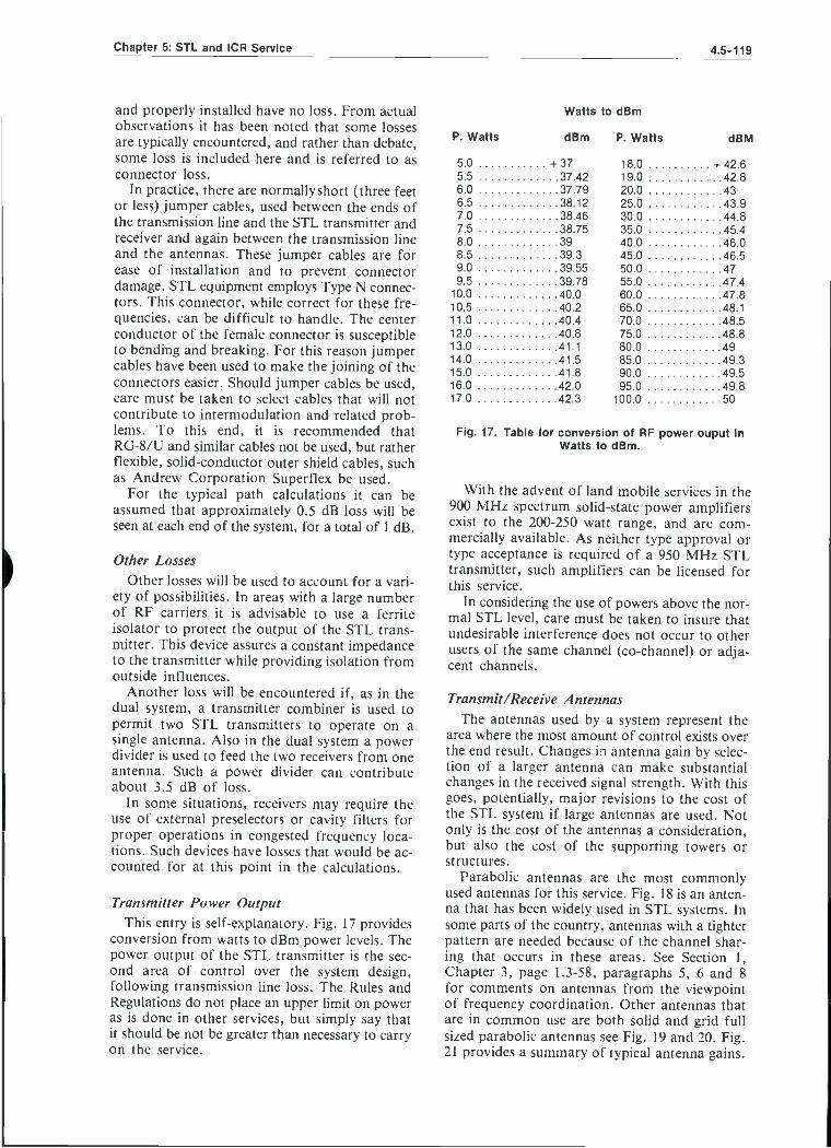
Chapter 5: STL and ICR Service 4.5 -119
and properly installed have no loss. From actual observations it has been noted that some losses are typically encountered, and rather than debate, some loss is included here and is referred to as connector loss.
In practice, there are normally short (three feet or less) jumper cables, used between the ends of the transmission line and the STL transmitter and receiver and again between the transmission line and the antennas. These jumper cables are for ease of installation and to prevent connector damage. STL equipment employs Type N connec- tors. This connector, while correct for these fre- quencies, can be difficult to handle. The center conductor of the female connector is susceptible to bending and breaking. For this reason jumper cables have been used to make the joining of the connectors easier. Should jumper cables be used, care must be taken to select cables that will not contribute to intermodulation and related prob- lems. To this end, it is recommended that RG -8 /U and similar cables not be used, but rather flexible, solid- conductor outer shield cables, such as Andrew Corporation Superflex be used.
For the typical path calculations it can be assumed that approximately 0.5 dB loss will be seen at each end of the system, for a total of 1 dB.
Other Losses Other losses will be used to account for a vari-
ety of possibilities. In areas with a large number of RF carriers it is advisable to use a ferrite isolator to protect the output of the STL trans- mitter. This device assures a constant impedance to the transmitter while providing isolation from outside influences.
Another loss will be encountered if, as in the dual system, a transmitter combiner is used to permit two STL transmitters to operate on a single antenna. Also in the dual system a power divider is used to feed the two receivers from one antenna. Such a power divider can contribute about 3.5 dB of loss.
In some situations, receivers may require the use of external preselectors or cavity filters for proper operations in congested frequency loca- tions. Such devices have losses that would be ac- counted for at this point in the calculations.
Transmitter Power Output This entry is self -explanatory. Fig. 17 provides
conversion from watts to dBm power levels. The power output of the STL transmitter is the sec- ond area of control over the system design, following transmission line loss. The Rules and Regulations do not place an upper limit on power as is done in other services, but simply say that it should be not be greater than necessary to carry on the service.
Watts to dBm
P. Watts dBm P. Watts dBM
5.0 +37 18.0 + 42.6 5.5 37.42 19.0 42.8 6.0 37.79 20.0 43 6.5 38.12 25.0 43.9 7.0 38.46 30.0 44.8 7.5 38.75 35.0 45.4 8.0 39 40.0 46.0 8.5 39.3 45.0 46.5 9.0 39.55 50.0 47 9.5 39.78 55.0 47.4
10.0 40.0 60.0 47.8 10.5 40.2 65.0 48.1 11.0 40.4 70.0 48.5 12.0 40.8 75.0 48.8 13.0 41.1 80.0 49 14.0 41.5 85.0 49.3 15.0 41.8 90.0 49.5 16.0 42.0 95.0 49.8 17.0 42.3 100.0 50
Fig. 17. Table for conversion of RF power ouput in Watts to dBm.
With the advent of land mobile services in the 900 MHz spectrum solid -state power amplifiers exist to the 200 -250 watt range, and are com- mercially available. As neither type approval or type acceptance is required of a 950 MHz STL transmitter, such amplifiers can be licensed for this service.
In considering the use of powers above the nor- mal STL level, care must be taken to insure that undesirable interference does not occur to other users of the same channel (co- channel) or adja- cent channels.
Transmit /Receive Antennas The antennas used by a system represent the
area where the most amount of control exists over the end result. Changes in antenna gain by selec- tion of a larger antenna can make substantial changes in the received signal strength. With this goes, potentially, major revisions to the cost of the STL system if large antennas are used. Not only is the cost of the antennas a consideration, but also the cost of the supporting towers or structures.
Parabolic antennas are the most commonly used antennas for this service. Fig. 18 is an anten- na that has been widely used in STL systems. In some parts of the country, antennas with a tighter pattern are needed because of the channel shar- ing that occurs in these areas. See Section 1, Chapter 3, page 1.3 -58, paragraphs 5, 6 and 8 for comments on antennas from the viewpoint of frequency coordination. Other antennas that are in common use are both solid and grid full sized parabolic antennas see Fig. 19 and 20. Fig. 21 provides a summary of typical antenna gains.

4.5 -120
Fig. 18. Scala PR -450U STL antenna. A commonly used STL antenna. Antenna shown is in use at
KPDJ -FM Eureka, California. (Courtesy Broadcast Engineering)
Fig. 19. Typical grid Parabolic STL antenna. Grid antennas provide gain without the wind loading of
solid dish antennas. (Courtesy Anixter -Mark)
Section 4: Program Transmission Facilities
Other Gains While not common in many STL systems, there
are devices that can be included that will result in further increases in total system gain. These include preamplifiers that may be used ahead of the STL receiver to lower the receiver noise figure and increase its sensitivity, thus adding gain but with a penalty of increased cross and inter - modulation. In the dual STL or other situations where more than one receiver is located at the transmitter site, a receiver multicoupler may be used to couple these receivers to one antenna.
Fig. 20. Sol d parabolic STL antenna. This type of antenna provides excellent side and back
lobe protection and is used in situations involving channel sharing.
(Courtesy Andrew Corporation)
TYPE
Grid Parabolic Antenna
Forward Gain (dBi)
4 foot diameter 18.9 6 foot diameter 22.0 8 foot diameter 25.0
10 foot diameter 27.0 12 foot diameter 28.5 15 foot diameter 30.0
Solid Parabolic Antenna 4 foot diameter 18.7 6 foot diameter 22.3 8 foot diameter 24.8
10 foot diameter 26.7 12 foot diameter 28.3 15 foot diameter 30.2
Parabloic, Single Plane, Grid a foot x 6 foot 20.1
Source - Manufacturers data sheets. Data to be considered typical, only.
Fig. 21. Chart of antenna forward gains for commonly used STL antennas.
Some multicouplers contain preamplifiers to com- pensate for the loss in the power dividers used for this division, and these can contribute gain to the overall system.
Expected Received Signal Strength This number, expressed in dBm, is the end re-
sult of these calculations. It is, as the name im- plies, the anticipated RF energy entering the receiver RF input connector. As the microvolt (SV) is the unit of measure more commonly used in this area, the above form provides space to
Chapter 5: STL and ICR Service 4.5 -121
enter the end result in this unit. Fig. 22 provides a table for conversion to µV from dBm.
Desired Signal Level This parameter expressed in µV and dBm
represents a given sensitivity specification for the selected STL receiver. As the desired service of the STL system is to deliver the program audio or signal to the transmitter site, a measurement of program signal -to -noise ratio (SNR) seems more appropriate than a quieting figure or other receiver sensitivity measurement. It is customary to use 60 dB SNR, but with the improving noise floors of program sources, transmitters, and other components of the program chain in FM service this figure may have to be increased to 70 dB. In a situation where there is co- channel sharing of the selected channel, the performance of the receiver to produce the desired SNR under co- channel conditions must be taken into considera- tion. Such co- channel operation will typically in-
MICROVOLTS DBM MICROVOLTS DBM 0.10 -127 35 - 76 0.12 - 125.25 40 - 74.9 0.14 - 124 45 - 73.9 0.16 - 122.9 50 - 72.9 0.18 - 121.9 60 - 71.25 0.20 - 120.9 70 - 70 0.25 - 119 80 - 68.9 0.30 - 117.25 90 - 67.9 0.35 -116 100 - 66.9 0.40 - 115 120 - 65.25 0.45 - 113.9 140 - 64 0.50 - 112.9 160 - 62.9 0.60 - 111.25 180 -61.9 0.70 - 110 200 - 60.9 0.80 - 108.9 250 - 59 9.90 -107.9 300 - 57.50 1.0 - 106.9 350 - 56 1.2 - 105.25 400 - 54.9 1.4 - 104 450 - 53.9 1.6 - 102.9 500 - 52.9 1.8 -101.9 600 -51.25 2.0 - 100.9 700 - 50 2.5 - 99 800 - 49 3.0 - 97.5 900 - 48 3.5 - 96 1,000 - 46.9 3.0 - 95 1,200 - 45.25 4.5 - 93.9 1,400 - 44 5.0 - 92.9 1,600 - 42.9 6.0 -91.25 1,800 -41.9 7.0 - 90 2,000 - 40.9 8.0 - 88.9 2,500 - 39 9.0 - 87.9 3,000 - 37.25
10 - 86.9 3,500 - 36 11 - 86 4,000 - 34.9 12 - 85.25 4,500 - 33.9 14 - 84 5,000 - 33 16 - 82.9 6,000 - 31.25 18 -81.9 7,000 - 30 20 - 80.9 8,000 - 28.9 25 - 79 9,000 - 27.9 30 - 77.25 10,000 - 26.9
Fig. 22. Microvolt to dBm conversion table, at 50 Ohms.
crease the desired signal level. In obtaining this number care must also be exercised to insure that the entire environment the receiver will see, be taken into consideration. This can be a considera- tion of all signals reaching the front -end of the receiver, levels of undesired signals in adjacent channels, in addition to any co- channel energy.
Fade Margin The last entry on this form may be the most
difficult to determine. This represents the signal level above the acceptable minimum that it is desired to have as normal to the RF input to the receiver. It is this number that the calculations are to produce. By selecting a minimum fade margin, antenna gains and transmission line losses can be selected to meet the desired fade margin.
One way this may be addressed is the amount of time through a year that it would be accept- able for the performance of the system to drop below the established minimum. This may be ex- pressed as a percentage of outage. Fig. 23 pro- vides the relationship of reliability and outage time.
As the numbers imply, when reliability is highest the outages are the shortest. In the Chapter on Frequency Coordination (Section 1, Chapter 3, page 1.3 -58, paragraph 4) it is sug- gested that 30 dB is a workable fade margin. For another point of view on this subject, Fig. 24 presents a nomograph relating distance to desired fade margin. It is the system design engineer's choice as to the level to be used for this entry in the calculations.
A Sample of Path Calculations Fig. 25 represents a completed, typical path cal-
culation. This theoretical path is some 10 miles in length, and uses parameters common to many situations. Having filled in the various gains and losses, they are totaled on the appropriate line. The Expected Received Signal Strength is ob- tained from the difference between Total System Loss and Total System Gain. The Fade Margin is the difference between this Expected Signal Level and the Desired Signal Level. It is to be noted that units of measure are not followed as an absolute with a mixing of dB, dBm, and dBi. As these are all relative, the desired end result is produced.
Repeaters The above analysis may produce a situation
that is not a workable STL configuration. If this is due to a blockage of the path than a repeater may be the solution. The two types of repeaters that may be considered at these frequencies are:
Active Inactive or Passive

4.5 -122 Section 4: Program Transmission Facilities
Reliability 0
90
99
99.99 99.999 99.999
120
Outage Time
07o
100
10
1
0.01
0.001 0.0001
45
40 110 -r
Outage Time per -
Year 8760 hrs
876 hrs 88 hrs 53 minutes
5.3 minutes 32 seconds
Month 720 hrs
72 hrs 7 hrs 4.3 minutes
26 seconds 2.6 seconds
Fig. 23. Reliability vs outage time.
100 35
90 - 30
aa ^o
°
U
60 < 1= 20
50 T <
15 ¡a1
40 O - < -. w
80
70 25
30 10
20
10
5
o o
Fig. 24. Commonly used fade margin reguirements versus path length. (Courtesy Broadcast Engineering)
Active Repeaters This type of repeater can be subdivided into
two types, that of a booster station and a full power repeater. The booster station is a station that receives and amplifies the signals of the originating station and re- transmits them on the same frequency without significantly altering them in any way. With a booster, the licensee is responsible for correcting any condition of interference that results from the radiation of radio frequency energy outside the assigned chan- nel. In essence, this permits a repeater station to be created that must function as an on- frequency repeater, or what might be called an active beam-
Day 24 hrs
2.4 hrs 14.4 minutes 8.6 seconds 0.86 seconds 0.086 seconds
LOSS 1. Path (10 miles /16.1 km) 2. Transmission Line (Total -400
feet /122 m)* 3. Connector (total) 4. Others -none
TOTAL SYSTEM LOSS
GAIN 5. Transmitter Power Output (15W) 6. Transmit Antenna" 7. Receive Antenna" 8. Others none
TOTAL SYSTEM GAIN
TOTAL SYSTEM LOSS TOTAL SYSTEM GAIN
Expected Received Signal Strength (3300 uV)
Desired Signal Level (100 uV for 70 dB SNR)
Fade Margin
- 116.0 dB
- 5.6 dB - 1.0dB
dB
- 122.6 dB
+ 41.8 dBm + 22.0 dBi + 22.0 dBi + dB
+ 85.8 dB
- 122.6 dB + 85.8 dB
- 36.8 dBm
- 66.9 dBm
+ 30.1 dB
Notes: ' -7/8 low -loss foam transmission line " -6 foot grid parabolic antennas
Fig. 25. Example of a typical STL path calculation, reflecting a path length of 10 mile.
bender. A waiver is required for a booster sta- tion, that operates in conjunction with any STL /ICR system.
The second type of repeater is more conven- tional. This is normally a standard STL receiver feeding an STL transmitter, with different input and output frequencies or channels. For this, an ICR license is needed as it is an additional sta- tion. This repeater functions as a baseband repeater, with program output of the receiver feeding the program input of the repeater trans- mitter. Recently one firm offered a commercial I.F. or intermediate frequency STL repeater,

Chapter 5: STL and ICR Service 4.5 -123
similar to those used in telephony microwave systems. In establishing a two hop system with a repeater, it can treated as two individual paths for purposes of path calculations.
Inactive or Passive Repeaters At 950 MHz this type of repeater is used, but
only under certain conditions. See Section 4, Chapter 2, Microwave Engineering for the Broad- caster, page 4.2 -68 for details on true passive repeaters. With the billboard type passive re- peater, normally the physical size at 950 MHz is so large making it not physically or financially viable. This is not to imply that the passive repeater should be ignored, as there are situations where it can be the ideal solution. Another passive repeater is back -to -back antennas. In consider- ing the configuration, performance can be calcu- lated as was done above, but using the expected received signal strength from the "receiving" antenna as the transmitter power output for the second hop calculations. From a mathematical viewpoint it will be seen that it will require a very short path for back -to -back antennas to function successfully as a passive repeater.
REFERENCES 1. Hamsher, Communications System Engineer-
ing Handbook, McGraw -Hill. 2. Reference Data for Radio Engineers, ITT -
Howard W. Sams and Co.
3. Leukurt Electric Company, Engineering Con- siderations for Microwave Communications Systems, San Carlos, California.
4. Fink, Donald G., Electrical Engineers Hand- book, McGraw -Hill.
5. Saveskie, Peter N., Radio Propagation Handbook, Tab Books.
6. Siemens and Halske Aktiengesellschaft, Plan- ning and Engineering of Radio Link Paths, Munich, Germany.
7. Decible Products, About Combiners, Dallas, Texas.
8. Decible Products, About Selective Cavities, Dallas, Texas.
9. National Association of Broadcasters, Engi- neering Handbook, 7th edition sections 1, 3, and 4.

1