1 performance analysis of single receiver matched-mode

1

Performance Analysis of Single Receiver

Matched-Mode Localization

Yann Le Gall, Francois-Xavier Socheleau, Member, IEEE and Julien Bonnel, Member, IEEE

Abstract

Acoustic propagation in shallow water at low frequency is characterized by a few propagating modes.

When the source is impulsive or short enough, the modes can be extracted from the signal received

on a single sensor using a warping operator. This opens the door to single receiver matched-mode

processing (SR-MMP) as a means to estimate source location and/or ocean environmental parameters.

While the applicability of SR-MMP has been demonstrated through several experiments, prediction of its

achievable performance has not been fully investigated. In this paper, performance analysis of SR-MMP

is carried out using numerical simulations of a typical shallow water environment, incorporating possible

environmental mismatch as well as degradations resulting from non-ideal modal filtering. SR-MMP is a

non-linear estimation problem that presents three regions of operation: the high SNR asymptotic region

driven by local errors, the intermediate SNR threshold region driven by sidelobe ambiguities and the

low SNR no-information region. The method of interval errors, which gives computationally efficient

and reliable mean squared error performance prediction, is used to conduct the analysis. The results

suggest that the SR-MMP performance depends strongly on the source/receiver depth. A significant loss

in performance is observed when the receiver is located at a node common to two modes. Receiver

depth must therefore be chosen with care. SR-MMP seems to be quite robust to mismatch on the seabed

properties alone but does not handle well the combined effect of seabed and water column mismatches.

Non-ideal modal filtering has a moderate impact on performance.

Index Terms

Underwater acoustics, matched-field processing, matched-mode processing, performance analysis,

method of interval errors

Yann Le Gall is with Thales Underwater Systems, Route de Saint Anne du Portzic, Brest, France (e-mail:

[email protected]). Francois-Xavier Socheleau is with IMT Atlantique, Lab-STICC, UBL, Technopole Brest-Iroise

CS83818, Brest 29238, France, France (e-mail: [email protected]). Julien Bonnel is with the Woods Hole

Oceanographic Institution, Woods Hole, MA 02543 USA (e-mail: [email protected])

November 6, 2017 DRAFT

2

I. INTRODUCTION

Matched-field processing (MFP) has been a topic of great interest for the underwater acoustic commu-

nity over the past decades [1]. From data collected on an array of sensors, MFP allows the estimation of

source position and/or environmental parameters by maximizing a cost function called the processor that

quantifies the match between the recorded acoustic field and simulated replicas of the acoustic field. At

low-frequency in shallow water, the propagation can be described by normal mode theory [2, Ch. 5] and

the acoustic field consists of several propagating modes. When the source signal is impulsive or at least

short enough, these modes can be extracted from the signal received on a single receiver using a warping

operator [3]–[6]. This operation is called single receiver modal filtering. It has recently been extended to

(unknown) frequency modulated source signals [7], [8]. Once modes are filtered, whether the source is

impulsive or frequency modulated, matched-mode processing (MMP) [9]–[11] can be applied to infer the

desired parameter values. When using a single hydrophone, this is referred to as single-receiver MMP

(SR-MMP) and is the focus of this paper. SR-MMP is different from classical MMP, which applies in a

more general context but requires a vertical array spanning most of the water column to filter the modes

[10], [12], [13].

Unlike MFP that considers the total pressure field, MMP explicitly compares the measured modes

to simulated mode replicas to estimate the desired parameter values. Working in mode space has the

additional advantage of providing physical insight into the estimation scheme which makes it easier to

deal with problems such as environmental mismatch [9], [10], [14]. Most modal-based single-receiver

inversion algorithms considering transient sources are based on the time-frequency (TF) dispersion of

the modes [15]–[17]. These methods allow the estimation of the source/receiver range and some of the

seabed geoacoustic properties such as sound speed and density. However, because they are based on

the position of the modes in the TF domain (i.e. the TF dispersion curves), these methods are only

sensitive to the mode phase. They are thus unable to estimate source depth and/or seabed attenuation

which are intrinsically related to mode amplitudes. To estimate such parameters, it is required to properly

filter the modes and inject their amplitude into the inverse problem. For example, seabed attenuation can

be estimated through the study of mode amplitude ratios [18], [19]. Alternatively, SR-MMP takes into

account both mode phase and mode amplitude information. If the source signal is perfectly known, it is

possible to use the absolute phase and amplitude through a coherent MMP processor. However, this is

not possible in a source localization scheme, where the source is inherently unknown. When the source

signal is unknown, it is possible to use relative phase and amplitude information through an incoherent


3

modal processor. In the context of source localization, incoherent SR-MMP allows a joint estimation of

source depth and range [8], [20]. Only the incoherent case will be considered in the following.

While the applicability of SR-MMP has been demonstrated through several experiments [4], [8], [20]–

[23], prediction of its achievable performance remains an open question. SR-MMP performance prediction

is, in fact, quite challenging because, like MFP or array MMP methods, SR-MMP attempts to solve a

nonlinear inverse problem. Nonlinear parameter estimators are known to exhibit a multimodal structure

corresponding to sidelobes on the ambiguity surface that quantifies, in our case, the match between

measured and replica modes. Due to these sidelobes, SR-MMP performance is subject to the so-called

threshold effect [24]. That is, below a certain level of signal-to-noise ratio (SNR) or a certain sample size

called threshold, an abrupt increase of the estimator mean-square error (MSE) is observed. More generally,

MSE performance curves for nonlinear estimation typically exhibit three distinct regions as function of the

SNR: the “no information” region at very low SNR (driven by ambiguity errors), the asymptotic region at

high SNR (driven by mainlobe errors) and the threshold region in between that characterizes the transition

from global to local errors [25]. This behavior of MSE is well known [24], but accurate prediction of the

performance in the three regions is an open problem in general. A brute-force way to approximate this

performance is to resort to Monte-Carlo simulations but this comes at the price of very time-consuming

computer simulations. This is particularly true when errors due to sidelobes may rarely occur but may

have a significant impact on MSE. An alternative approach to Monte-Carlo simulation is to derive MSE

bounds or MSE approximations [26]–[33]. However, not all bounds or MSE approximations are suitable

for nonlinear problem performance predictions. The well known Cramer-Rao bound for example is only

tight in the high SNR asymptotic region. In this study, the performance of SR-MMP is analyzed through

an MSE approximation method called the method of interval errors (MIE). The MIE is designed to yield

approximate but reliable error prediction at all SNR regions in a computationally efficient way. The MIE

approximation recently derived for MFP performance prediction in [32], [33] under a signal model where

the source signal is assumed deterministic unknown is used here for SR-MFP performance analysis. It

also allows consideration of realistic situations where the SR matched-mode processors have inaccurate

or incomplete information concerning the propagation environment, leading to a mismatch between the

actual physical modes and the replicas used to solve the inverse problem.

The paper is organized as follows. The matched-mode processing problem is introduced in a single

receiver context in Section II. The MIE approximation for SR-MMP performance prediction is presented

in Section III. Finally, numerical examples applied to source localization are presented in Section IV,

followed by conclusions in Section V.


4

Notation: Throughout this paper, lowercase boldface letters denote vectors, e.g., x, and uppercase

boldface letters denote matrices, e.g., A. The superscripts T and H mean transposition and Hermitian

transposition, respectively. The N×N identity matrix is denoted by IN . Finally, E{·} denotes expectation,

P(·) denotes the probability measure and δ is the Kronecker delta function.

II. SINGLE RECEIVER CONTEXT

A. Modal propagation and modal filtering

In the studied context, low-frequency sound in shallow water, propagation can be described by normal-

mode theory. Considering a broadband source emitting at depth zs in a range-independent waveguide,

the spectral component of the pressure field y(f) received at depth zr after propagation over a range rs

is given by [2, Ch. 5]:

y(f) = s(f)

M∑

m=1

xm(f), (1)

where s(f) is the source spectrum and M is the number of propagating modes. The quantity xm(f) is

the contribution of mode m to the pressure field. It is expressed as

xm(f) = Qψm(f, zs)ψm(f, zr)ejrskrm(f)

√

krm(f)rs, (2)

where krm and ψm are the horizontal wavenumber and modal depth function of mode m, respectively.

The quantity Q = ejπ/4√8πρ(zs)

represents a constant factor with ρ(zs) as the water density at the source

depth zs. For notational convenience, the dependencies in rs, zs and zr are dropped for xm(f).

To perform MMP, it is necessary to filter the modes. This operation can be done with a single receiver

using signal processing transformations known as warping operators [3]. A warping operator transforms

a signal y(t) into a new warped signal Why(t) using a warping function h(t):

Why(t) =√

|h′(t)|y[h(t)]. (3)

Note that warping is an invertible transformation, and that the inverse warping function is h−1(t). The

aim of warping is to linearize the phase of the signal y(f) and it can be adapted to any physical situation

by choosing the suitable h(t). Dispersion based warping has been introduced by Le Touze et al. [4]. Its

goal is thus to transform every mode into a single frequency (CW signal). To do so, one suitable warping

function is [4], [5], [17]

h(t) =√

t2 + t2r, (4)

with tr = r/cw where cw is an average water sound speed.


5

It has been demonstrated previously that warping defined in Eq. (4) is a robust transformation which can

be applied to most low-frequency shallow-water scenarios without precise knowledge of the environment

or the propagation range (tr can be determined empirically without knowing rs and cw) [5], [17]. It is

therefore adapted to the context of single receiver MMP and it allows modes to be filtered using the

following methodology (illustrated by Fig. 3 in [5])

1) warp the received signal using h(t),

2) go to the TF domain, filter warped mode m, and go back to the time domain,

3) unwarp mode m using h−1(t).

In the next sections, MMP performance will first be studied with and without environmental mismatch

assuming that the modes are perfectly filtered. The impact of non-ideal modal filtering on MMP perfor-

mance will then be illustrated in Sec. IV-F by considering the degradations resulting from this filtering

as an additional mismatch.

B. Data model

The goal of SR-MMP is to estimate an unknown parameter set θ from the modes recorded on a

single hydrophone. The parameter set θ may contain both source position (range, depth), and/or ocean

environmental parameters. Consider M modes received on a single receiver. The complex received signal

is modeled by the M × 1 vector

y(fk) = s(fk) · x(fk,θ) +w(fk), k = 1, ...,K (5)

where,

• K is the number of available frequencies fk.

• x(fk,θ) is a complex M × 1 vector representing the contribution of M modes at frequency fk. The

m-th component of x(fk,θ) is given by Eq. (2).

• s(fk) is a deterministic complex scalar representing the source amplitude and phase.

• w(fk) is a complex M × 1 vector representing circularly-symmetric, zero mean Gaussian noise that

is independent of the source signal. In addition, the noise is assumed to be white across both modes

and frequencies, so that

E{

w(fk1)wH(fk2

)}

= σ2w(fk1

)IMδfk1 ,fk2 , (6)

and the noise power σ2w(fk) is assumed to be known for each frequency fk. The assumption of

circularly-symmetric uncorrelated Gaussian noise is an approximation. Modal filtering may affect


6

these properties. However, numerical experiments (not shown here) conducted with the modal filters

used in Sec. IV-F suggest that for the results presented herein such an assumption is a reasonable

approximation.

The set of observations is collected in the following vector

y = [yT (f1), yT (f2), . . . yT (fK)]T . (7)

C. Matched-mode processors

The inverse problem modeled by (5) is commonly solved by maximizing a cost function, known as

the matched-mode processor, that quantifies the match between measured and simulated replica modes.

A common approach for deriving such processors is to resort the maximum likelihood (ML) framework

[34], [35]. ML estimation is known to offer the best asymptotic properties with respect to efficiency and

can be applied for any state of source spectral knowledge [35].

Let p(y|θ) denote the conditional probability density function (pdf) of the observation y given the

source/environmental parameter set θ. According to the observation model of Section II, this pdf satisfies

p(y|θ) =1

∏Kk=1|πσ

2w(fk)|M

K∏

k=1

exp

(

−|y(fk)− s(fk)x(fk,θ)|

2

σ2w(fk)

)

. (8)

The maximum likelihood estimate of the desired parameter set θ is obtained by maximizing (8) with

respect to θ, considering the source signal s(fk) as a nuisance parameter that is replaced by its ML

estimate according to the profile likelihood technique [36].

In the case where no information is available on the sequence s(fk) and in the absence of mismatch

between the actual modes and the simulated replicas, the ML estimate of the desired parameter set θ is

[35]

θ = argmaxθ

C (θ) , with C (θ) =

K∑

k=1

|xH(fk,θ)y(fk)|2

σ2w(fk)

, (9)

where x(fk,θ) is a normalized version of x(fk,θ) defined as x(fk,θ) =x(fk,θ)

‖x(fk,θ)‖ . This MMP is referred

to as incoherent because the multiple frequencies are summed incoherently, i.e., with the absolute value

that cancels phase information inside the double sum.

In practice, when solving the inverse problem (9), MMP methods may have inaccurate or incomplete

information about the oceanic waveguide and the modes may be imperfectly filtered. Consequently, there

may be a mismatch between the actual extracted modes and the replicas produced by a numerical model.

The sensitivity to environmental mismatch or non-ideal mode filtering can be of particular concern for

MMP and a quantitative assessment of its effect on performances is of prime importance. Formally, in


7

presence of mismatch, the assumed modes xǫ(fk,θ) used to estimate θ differ from the extracted modes

x(fk,θ) and the cost function used in (9) is then expressed as

C (θ) =

K∑

k=1

|xHǫ (fk,θ)y(fk)|

2

σ2w(fk)

, (10)

where xǫ(fk,θ) =xǫ(fk,θ)

‖xǫ(fk,θ)‖ .

III. METHOD OF INTERVAL ERRORS

The MSE of nonlinear estimators is explicitly connected to the shape of the ambiguity function (AF)

which quantifies the match between measured and replica modes. Formally, if the true set of parameters

is denoted as θ0, the AF corresponds to the function C(θ) with a noise-free observation and is expressed

as:

ψ(θ) =

K∑

k=1

γ(fk)|xǫ(fk,θ)H x(fk,θ0)|

2, (11)

where γ(fk) =|s(fk)|2σ2w(fk)

‖x(fk,θ0)‖2. For non-linear estimation problems, the ambiguity function exhibits

a mainlobe/sidelobe behavior and the MSE presents three regions of operation as a function of SNR: the

high SNR asymptotic region driven by mainlobe errors, the intermediate SNR threshold region where there

is a strong increase in MSE due to sidelobe errors (also called outliers) and the low SNR no-information

region (see Figure 1).

1000 2000 3000 4000 5000 6000 7000 8000 90000

0.1

0.2

0.3

0.4

0.5

0.6

0.7

0.8

0.9

1

with mismatchwithout mismatch

Am

big

uity f

un

ctio

n

θ

θ0 θmis

SNR (dB)

MSE (

dB)

MSE without mismatch

Asymptotic

regionThreshold

region

No-information

region

Threshold SNR

MSE with mismatch

(a) (b)

Fig. 1. Schematic illustration of: (a) the ambiguity function (11) at infinite SNR and (b) MSE regions of a non-linear estimator.

(a) is obtained by setting γ(fk) to a constant value, for all k, such that ψ(θ0) = 1 in the absence of mismatch. When there is

no mismatch and no measurement error, the maximum of the ambiguity function is at the true parameter set θ0. When there is

mismatch the estimator can be biased at infinite SNR and the maximum of the ambiguity function is at a value θmis 6= θ0.


8

MIE provides accurate MSE prediction of nonlinear estimators (see the tutorial treatment by Van Trees

and Bell in [37]). MIE builds upon the decomposition of the MSE into two terms: the local errors that

concentrate around the mainlobe peak and outliers that concentrate around the sidelobe peaks. Consider

the true parameter θ0 and a discrete set of No parameter points {θ1,θ2 . . . θNo} sampled at the sidelobe

maxima of the AF. The conditional MSE of the ML estimator can then be approximated as [25], [30],

[38]–[40]:

Ey

{

(θ − θ0)(θ − θ0)T}

≈

(

1−

No∑

n=1

Pe(θn|θm)

)

× MSE(asymp)(θ0)

+

No∑

n=1

Pe(θn|θm)× (θn − θ0)(θn − θ0)T , (12)

where θm denotes the parameter set that maximizes the AF (see Figure 1, when there is no mismatch

θm = θ0 and when there is mismatch θm = θmis). Pe(θn|θm) is the pairwise error probability of the

ML estimator (9) possibly under model mismatch (10), i.e. the probability of deciding in favor of the

parameter θn in the binary hypothesis test {θn,θm}.

The pairwise error probability Pe(θn|θm) is used as an approximation of the probability that the

estimate falls on the sidelobe n and (1−∑No

n=1 Pe(θn|θm)) is used as an approximation of the probability

that the estimate falls on the mainlobe (i.e. the probability of local errors). MSE(asymp)(θ0) is the

asymptotic MSE of the ML estimator. In the absence of mismatch, the CRB is usually a good predictor of

the performance in this region [32]. Since mismatch is possible, these local errors must be approximated

by other means. Analytic expressions for Pe(θn|θm) and MSE(asymp)(θ0) have recently been derived [33].

The analytic expressions of Pe(θn|θm) and MSE(asymp)(θ0) are summarized in Appendices A and B.

IV. PERFORMANCE ANALYSIS

In this section, the performance of SR-MMP source localization is analyzed in a conventional applica-

tion framework using MIE. The accuracy of SR-MMP is first studied in the absence of model mismatch

for several source and receiver positions. Next, the impact of mismatch between the assumed and the

true environments is examined. Finally, the impact of mode filtering on the performance is evaluated.

The performance metrics used for the analysis are:

• The MSE in decibel: (MSE)dB = 10 log10

(

E

{

|θ − θ0|2})

.

• The root mean square error: RMSE =

√

E

{

|θ − θ0|2}

.

• The threshold SNR (formally defined in Sec. IV-D).


9

Depending upon the context, θ (resp. θ0) either refers to the estimated (resp. true) value of rs or zs. In

all the studied scenarios, both the source range and depth are assumed unknown.

A. Scenarios

The simulation scenarios considered here are illustrated in Fig. 2. The true environment is made of

a water column of height D = 79 m, a sound speed profile with a thermocline and a seabed with two

sediment layers over a bottom halfspace. The geoacoustic properties of the seabed are shown in Fig.

2 and the values of the sound speed profile are listed in Table I. We consider K = 50 frequencies

uniformly spaced in the bandwidth ∆f = [25, 150] Hz and M = 4 propagating modes. The SNR is

defined as SNR(fk) =|s(fk)|2‖x(fk,θ0)‖2

σ2w(fk)

and is constant across frequencies. The search interval for the

source position is set (in meters) to (rs, zs) ∈ [500, 10000] × [5, 75].

sound speed (m/s)

1500 1600 1700 1800

de

pth

(m

)

0

20

40

60

80

100

120

True environment

sound speed (m/s)

1500 1600 1700 1800

0

20

40

60

80

100

120

Environment B

sound speed (m/s)

1500 1600 1700 1800

0

20

40

60

80

100

120

Environment C

cw

(z) cw

(z) cw

water column water column water column

sediment 2 :h

2 = 15 m

cl2

= 1600 m/s

ρl2

= 1.6 g/cm3

αl2

= 0.5 dB/λsediment 1 :h

1 = 5 m

cl1

= 1650 m/s

ρl1

= 1.7 g/cm3

αl1

= 0.5 dB/λ

basement : cb = 1850 m/s

ρb = 1.9 g/cm3

αb = 0.5 dB/λ

basement :c

bb = [1575 1675] m/s

ρbb

= 1.9 g/cm3

αbb

= 0.5 dB/λ

basement :c

bc = [1575 1675] m/s

ρbc

= 1.9 g/cm3

αbc

= 0.5 dB/λ

Fig. 2. True environment and and mismatched environments.

In practice, the actual propagation medium is not known perfectly. The detailed structure of the seabed

as well as its properties cannot be guessed accurately a priori if geoacoustic inversion campaigns have

not been conducted in advance. The sound speed profile is easier to measure (using CTD sensors for

instance) but its values may not always be available. Localization is then performed on the basis of

an assumed environment that is different from the real one. To assess the impact of such mismatch,

two environments are introduced: the B and C environments described in Fig. 2. Environment B is

representative of a significant lack of knowledge of the bottom properties. The sound speed profile in the

water column is the same as the true one but the seabed is simply made of a bottom halfspace with a


10

constant sound speed cbb. Several values of cbb between 1575 and 1675 m/s will be tested. Environment

C is representative of a significant lack of knowledge of the sound speed profile in the water column

as well as in the seabed. The sound speed profile in the water column is mistakenly assumed constant

at cw = 1494.9 m/s and the seabed is identical to environment B. Several seabed sound speed values

between cbc = 1575 m/s and cbc = 1675 m/s will also be tested.

Depth z (m) 0 10 22 25 28 31 46 49 50 D

Sound speed cw(z) (m/s) 1525.7 1525.7 1487.8 1486.6 1484.1 1484.3 1487.9 1487.5 1488.0 1491.2

TABLE I

SOUND SPEED PROFILE IN THE WATER COLUMNS FOR THE TRUE ENVIRONMENT AND FOR ENVIRONMENT B.

B. Problem analysis

Fig. 3 shows some examples of AF in the absence of model mismatch. It can be seen that source

localization is a multimodal problem so that MIE is well adapted to this context.

The expression of a single mode, as given by (2), allows us to understand the SR-MMP localization

problem. Although the estimation of range and depth by MMP is a coupled problem, it should be noted

that the information on the depth of the source is carried by the modal function ψm(f, zs) while the

range information is mainly carried by the phase term ejrskrm(f). Fig. 4 shows the modal depth functions

at 100 Hz of the four filtered modes used to perform the SR-MMP localization. Some useful comments:

• The modal depth functions converge to a common node at the surface.

• The modal depth functions present some symmetry with respect to the center of the water column

(or antisymmetry depending on the modes parity) slightly distorted by the penetration in the bottom

and by the sound speed profile in the water column.

• The amplitudes of the modal depth functions of modes n = 2 and n = 4 cancel around the depth

z = 45 m.

• The four modes significantly penetrate into the sediment layers but not much into the basement.

These observations will ease the interpretation of some results obtained in the next sections. For instance,

the symmetry of modal functions already explains the shape of the AF in Fig. 3: an approximate axial

symmetry is observed with respect to the central depth of the water column.


11

(a) (b)

(c) (d)

Fig. 3. Examples of ambiguity functions of SR-MMP, (a) at rs = 5000 m and zs = 40 m, (b) at rs = 5000 m and zs = 25 m,

(c) at rs = 8000 m and zs = 40 m, (d) at rs = 3000 m and zs = 25 m, (in all cases zr = 20 m).


12

Ψ1

Ψ2

Ψ3

Ψ4

sound speed (m/s)

1400 1650 1900

de

pth

(m

)

0

20

40

60

80

100

sediment 1 :h

1 = 5 m

cl1

= 1650 m/s

ρl1

= 1.7 g/cm3

αl1

= 0.5 dB/λ

basement : cb = 1850 m/s

ρb = 1.9 g/cm3

αb = 0.5 dB/λ

sediment 2 :h

2 = 15 m

cl2

= 1600 m/s

ρl2

= 1.6 g/cm3

αl2

= 0.5 dB/λ

Fig. 4. Modal depths function of the true environment at 100 Hz (only the first four modes are represented).


13

C. Validation of MIE on a single point

The MIE approach is here validated by comparing its performance predictions with the results obtained

by Monte Carlo simulations. The simulations are performed for a single source position: rs = 5000 m

and zs = 40 m. Two cases are studied, a first case without mismatch and a case in presence of mismatch.

To show the accuracy of MIE, even when the asymptotic MSE is not dominated by the bias θm − θ0,

we here consider a slight mismatch where the assumed values for cl1 and cl2 in Fig. 2 are 1620 m/s

and 1570 m/s, respectively (instead of the true values cl1 = 1650 m/s and cl2 = 1600 m/s). Monte Carlo

simulations are run over Nc = 1000 iterations for each SNR. The choice of the parameter No, defined

in Sec. III, is based on the shape of the AF. It is set to No = 20 for all the simulations.

SNR (dB)-20 -15 -10 -5 0 5 10 15 20

Lo

ca

l M

SE

(d

B)

0

10

20

30

40

50

60

70(a) MSE on range

MIE with mismatch

MIE without mismatch

Monte-Carlo with mismatch

Monte-Carlo without mismatch

SNR (dB)-20 -15 -10 -5 0 5 10 15 20

Lo

ca

l M

SE

(d

B)

-20

-10

0

10

20

30(b) MSE on depth

MIE with mismatch

MIE without mismatch

Monte-Carlo with mismatch

Monte-Carlo without mismatch

Fig. 5. MIE and Monte-Carlo simulations at rs = 5000 m and zs = 40 m with and without model mismatch.

In both scenarios, a good match between Monte-Carlo simulations and MIE predictions is observed,

which validates the use of MIE for this problem. Note that it took a couple of days to get the results

of Monte Carlo simulations using Matlab with a contemporary work station (3 GHz CPU with 8 Gb

of RAM), whereas MIE provided its results only after a few seconds. Monte Carlo simulations are

computationally demanding because they require a large number of realizations and also because the

search grid in (rs, zs) must be very tight at high SNR to get accurate MSE estimations. In the next

sections, the simulations are carried for several environments and a large number of source positions.

Therefore, a Monte Carlo approach cannot be used to conduct the analysis (even though the speed could

be increased by running the simulations on a parallel cluster or using Fortran/C++ instead of Matlab,

it may take days/weeks to obtain the desired results); hence the interest of MIE. In the following, the

performance is assessed using MIE only.


14

D. Performance without environmental mismatch

Performance is first evaluated without environmental mismatch, i.e. both data and replica are simulated

in the same environment (A). The MIE is computed over the following search space:

• rs ∈ [500, 10000] m with 500 m steps,

• zs ∈ [5, 75] m with 4 m steps.

Overall, the MIE is evaluated using Nl ≈ 300 source positions.

In Fig. 6, the MIE analysis is averaged over the Nl positions so that the MSE can be evaluated for

several SNRs. Several receiver depths zr are also considered. For zr = 20 m and zr = 70 m, performances

are nearly equivalent. In both cases, the threshold SNR is around 6 dB and the MSEs are similar. However,

the performance decreases for zr = 43 m. The threshold SNR is around 15 dB and the MSE is higher

both in the asymptotic region and in the threshold region. As stated in IV-B, the depth functions of

modes 2 and 4 have a node at about zr = 43 m (see Fig. 4). Because of this phenomenon, only modes

1 and 3 carry information that can be used by the SR-MMP receiver, which explains the relatively poor

performance. In general, if the receiver depth zr /∈ [40, 50] m, then the SR-MMP performances are similar

to the ones obtained for zr = 20 m or zr = 70 m. This illustrates the importance of the receiver depth

for SR-MMP. In general, we recommend avoiding modal nodes. In the following, the receiver depth is

set to zr = 20 m.

SNR (dB)

-20 -10 0 10 20

Glo

ba

l M

SE

(d

B)

0

10

20

30

40

50

60

70(a) MSE on range

zr=20 m

zr=43 m

zr=70 m

RMSE = 1000 m

RMSE = 100 m

RMSE = 10 m

RMSE = 3.2 m

SNR (dB)

-20 -10 0 10 20

Glo

ba

l M

SE

(d

B)

-10

0

10

20

30(b) MSE on depth

zr=20 m

zr=43 m

zr=70 m

RMSE = 10 m

RMSE = 3.2 m

RMSE = 1 m

RMSE = 0.56 m

Fig. 6. SR-MMP performance for rs ∈ [500, 10000] m and zs ∈ [5, 75] m for several receiver depths zr .

The global MSE (as presented in Fig. 6) reflects the average SR-MMP performance over the search

space (Nl ≈ 300 source positions). However, performance may vary depending on the source position.

To quantify this, the performance can be assessed for each source position. Fig. 7 presents several


15

performance metrics in the (zs, rs) domain. In particular, this figure shows the threshold SNR, the MSE

in the threshold region and the MSE in the asymptotic region. We define the threshold SNR as the lowest

SNR satisfying∑No

n=1 Pe(θn|θ0) > 10−4. Note that this definition will be used throughout the rest of the

paper. In other words, our threshold SNR is the minimal SNR for which the estimate has a probability

greater than 10−4 to be outside of the AF main lobe. The 10−4 value has been chosen empirically by

comparing∑No

n=1 Pe(θn|θ0) with the shape of the MSE versus SNR.

The threshold SNR quantifies the SNR below which the performance significantly decreases. However,

it does not quantify the performance deterioration. For a given SNR threshold, the error depends on the

distance (in range and in depth) between the mainlobe and the sidelobes. We then evaluate the MSE for

SNR=4 dB to study the performance in the threshold region. We also evaluate the MSE for SNR=20 dB

to evaluate the performance in the asymptotic region. As expected and as illustrated in Fig. 7, these

metrics depend on the source position.

First of all, the SNR threshold increases slightly when range rs increases. There are also particular

depths zs for which the SNR threshold is more important. These areas roughly correspond to modal depth

function nodes. In the threshold region (SNR=4 dB), the range MSE reflects the SNR threshold variations,

but the depth MSE behavior is more complicated. The depth MSE increases slowly with increasing rs but

the variations with zs differ. The error increases drastically when the source is not around the middle of

the water column. The approximate symmetry of the modal depth functions introduces an approximately

symmetric ambiguity increasing as zs moves closer to the interfaces (surface or seabed).

In the asymptotic region (SNR=20 dB), the range MSE also increases with rs and is high for particular

zs values (once again corresponding to modal depth function nodes). The depth MSE barely increases

with rs, but depends strongly on zs. It increases when the source is near the waveguide interfaces and

particularly when the source is near the sea surface. These high MSE values are due to the modal behavior

in these regions. Indeed, at such depths, the mode amplitude ratios change slowly so that source depth

estimation is difficult.


16

1 2 3 4 5 6 7 8 9

10

20

30

40

50

60

70

(a) Threshold SNR (dB)

depth

(m

)

range (km)

3

4

5

6

7

8

9

1 2 3 4 5 6 7 8 9

10

20

30

40

50

60

70

(b) MSE on range at 4 dB of SNR

de

pth

(m

)

range (km)

20

25

30

35

40

1 2 3 4 5 6 7 8 9

10

20

30

40

50

60

70

(c) MSE on depth at 4 dB of SNRd

ep

th (

m)

range (km)

0

5

10

15

1 2 3 4 5 6 7 8 9

10

20

30

40

50

60

70

(d) MSE on range at 20 dB of SNR

depth

(m

)

range (km)

2

4

6

8

1 2 3 4 5 6 7 8 9

10

20

30

40

50

60

70

(e) MSE on depth at 20 dB of SNR

depth

(m

)

range (km)

−20

−15

−10

−5

Fig. 7. (a) Threshold SNR, (b) range MSE with SNR=4 dB, (c) depth MSE with SNR=4 dB, (d) range MSE with SNR=20 dB

and (e) depth MSE with SNR=20 dB. Every pannel is computed over the search space rs ∈ [500, 10000] m and zs ∈ [5, 75] m.

Receiver depth is zr = 20 m.


17

E. Performance with environmental mismatch

The mismatch impact is evaluated for the two cases presented in Sec. IV-A. We first present the

performance when inversion is performed using environment B and then the performance when inversion

is performed using environment C. In both cases, data are simulated in environment A and the MIE is

computed over the following search space:

• rs ∈ [500, 10000] m with 500 m steps,

• zs ∈ [5, 75] m with 4 m steps.

Overall, the MIE is evaluated using Nl ≈ 300 source positions.

1) Inversion using environment B: As stated previously, environment B is representative of a significant

lack of knowledge of the seabed properties. Fig. 8 shows the global MSE for several seabed sound speed

values cbb (in environment B). For high SNRs, the MSE is obviously higher with seabed mismatch

than without, and the performances depend on the cbb value. The best performance is obtained for

cbb = 1625 m/s. This is expected as the modes are mainly affected by the first two sediment layers in

which cl1 = 1600 m/s and cl2 = 1650 m/s. Choosing cbb = 1625 m/s averages the speed of the first two

sediment layers and allows for a reasonably accurate approximation of the propagation (in our frequency

band). Except for the case cbb = 1575 m/s, the performance deterioration seems relatively minor: for

SNR greater than 7.5 dB, the RMSE in range is smaller than 316 m (MSE=50 dB) and smaller than

5.6 m in depth (MSE=15 dB), which is acceptable for most MMP source localization applications. The

threshold SNR remains around 6 dB and the MSE increase below this threshold approximately follows

the same rate as in the no-mismatch case.

SNR (dB)

-20 -10 0 10 20

Glo

ba

l M

SE

(d

B)

10

20

30

40

50

60

70(a) MSE on range

1575 m/s

1600 m/s

1625 m/s

1650 m/s

1675 m/s

no mismatch

RMSE = 1000 m

RMSE = 320 m

RMSE = 100 m

RMSE = 32 m

SNR (dB)

-20 -10 0 10 20

Glo

ba

l M

SE

(d

B)

-10

0

10

20

30(b) MSE on depth

1575 m/s

1600 m/s

1625 m/s

1650 m/s

1675 m/s

no mismatch

RMSE = 10 m

RMSE = 5.6 m

RMSE = 3.2 m

RMSE = 1.8 m

RMSE = 1 m

Fig. 8. Inversion using environment B. Global MSE over rs ∈ [500, 10000] m and zs ∈ [5, 75] m for several seabed sound

speeds cbb. Receiver depth is zr = 20 m.


18

Fig. 9 shows the SNR threshold, the range MSE at 20 dB and the depth MSE at 20 dB in the

(zs, rs) domain for a seabed speed cbb = 1625 m/s. Fig. 10 shows the same performance metrics but

for cbb = 1675 m/s. Comparing these figures with Fig. 7 nicely illustrates the mismatch impact and the

corresponding performance deteriorations.

In the case with mismatch, the MSE global trend is the same as in the case without mismatch. However,

several differences exist. Indeed, when considering mismatch, the MSE depends on the modes computed

in the true environment (A) and in the assumed environment (B). One should also note that different

seabed speeds lead to different performances. As an example, for cbb = 1625 m/s the worse performance

is found around zs = 20 m while it is found around zs = 50 m for cbb = 1675 m/s. Moreover, even if

cbb = 1625 m/s leads to the best average performance, there are source/SNR configurations where the

performance is better with cbb 6= 1625 m/s.

range (km)

1 2 3 4 5 6 7 8 9

de

pth

(m

)

10

20

30

40

50

60

70


5

10

15

20

range (km)

1 2 3 4 5 6 7 8 9

de

pth

(m

)

10

20

30

40

50

60

70


15

20

25

range (km)

1 2 3 4 5 6 7 8 9

de

pth

(m

)

10

20

30

40

50

60

70

(c) MSE on depth at 20 dB of SNR

-15

-10

-5

0

5

Fig. 9. Inversion using environment B. (a) Threshold SNR, (b) range MSE with SNR=20 dB, (c) depth MSE with SNR=20

dB. Every subfigure is computed over the search space rs ∈ [500, 10000] m and zs ∈ [5, 75] m. Receiver depth is zr = 20 m.

Seabed sound speed is cbb = 1625 m/s.


19

range (km)

1 2 3 4 5 6 7 8 9

de

pth

(m

)

10

20

30

40

50

60

70


5

10

15

20

range (km)

1 2 3 4 5 6 7 8 9

de

pth

(m

)

10

20

30

40

50

60

70


30

35

40

45

50

55

range (km)

1 2 3 4 5 6 7 8 9

de

pth

(m

)

10

20

30

40

50

60

70


-10

0

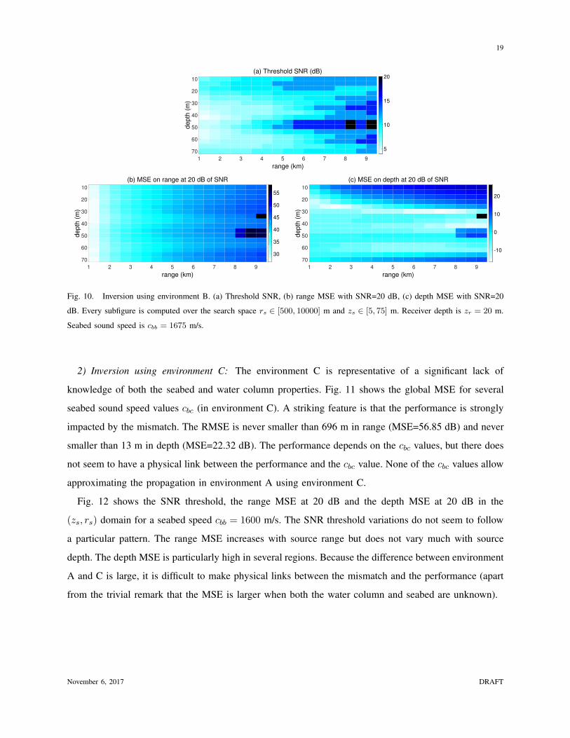
10

20

Fig. 10. Inversion using environment B. (a) Threshold SNR, (b) range MSE with SNR=20 dB, (c) depth MSE with SNR=20


Seabed sound speed is cbb = 1675 m/s.

2) Inversion using environment C: The environment C is representative of a significant lack of

knowledge of both the seabed and water column properties. Fig. 11 shows the global MSE for several

seabed sound speed values cbc (in environment C). A striking feature is that the performance is strongly

impacted by the mismatch. The RMSE is never smaller than 696 m in range (MSE=56.85 dB) and never

smaller than 13 m in depth (MSE=22.32 dB). The performance depends on the cbc values, but there does

not seem to have a physical link between the performance and the cbc value. None of the cbc values allow

approximating the propagation in environment A using environment C.

Fig. 12 shows the SNR threshold, the range MSE at 20 dB and the depth MSE at 20 dB in the

(zs, rs) domain for a seabed speed cbb = 1600 m/s. The SNR threshold variations do not seem to follow

a particular pattern. The range MSE increases with source range but does not vary much with source

depth. The depth MSE is particularly high in several regions. Because the difference between environment

A and C is large, it is difficult to make physical links between the mismatch and the performance (apart

from the trivial remark that the MSE is larger when both the water column and seabed are unknown).


20

SNR (dB)

-20 -10 0 10 20

Glo

bal M

SE

(dB

)

10

20

30

40

50

60

70(a) MSE on range

1575 m/s

1600 m/s

1625 m/s

1650 m/s

1675 m/s

no mismatch

RMSE = 1000 m

RMSE = 2500 m

SNR (dB)

-20 -10 0 10 20

Glo

bal M

SE

(dB

)

-10

0

10

20

30(b) MSE on depth

1575 m/s

1600 m/s

1625 m/s

1650 m/s

1675 m/s

no mismatch

RMSE = 13.3 m

RMSE = 18.8 m

Fig. 11. Inversion using environment C. Global MSE over rs ∈ [500, 10000] m and zs ∈ [5, 75] m for several seabed sound

speeds cbc. Receiver depth is zr = 20 m.

range (km)

1 2 3 4 5 6 7 8 9

de

pth

(m

)

10

20

30

40

50

60

70


10

15

20

25

30

range (km)

1 2 3 4 5 6 7 8 9

de

pth

(m

)

10

20

30

40

50

60

70


20

30

40

50

60

range (km)

1 2 3 4 5 6 7 8 9

de

pth

(m

)

10

20

30

40

50

60

70


-20

-10

0

10

20

Fig. 12. Inversion using environment C. (a) Threshold SNR, (b) range MSE with SNR=30 dB, (c) depth MSE with SNR=30


Seabed sound speed is cbc = 1600 m/s.

F. Impact of mode filtering

In this section, the impact of non-ideal mode filtering is evaluated by considering degradations resulting

from mode filtering as mismatch. Formally, we first simulate the time domain signal that contains all the

propagating modes. We then apply modal filtering using warping (see Sec. II-A) to obtain the extracted

modes x(fk,θ) and evaluate the performance when using the mode replicas xǫ(fk,θ) to carry inversion


21

with or without environmental mismatch. Because of the tedious non-automatic task of modal filtering,

the results presented here only correspond to a single source position (zs, rs) = (40 m, 5000 m).

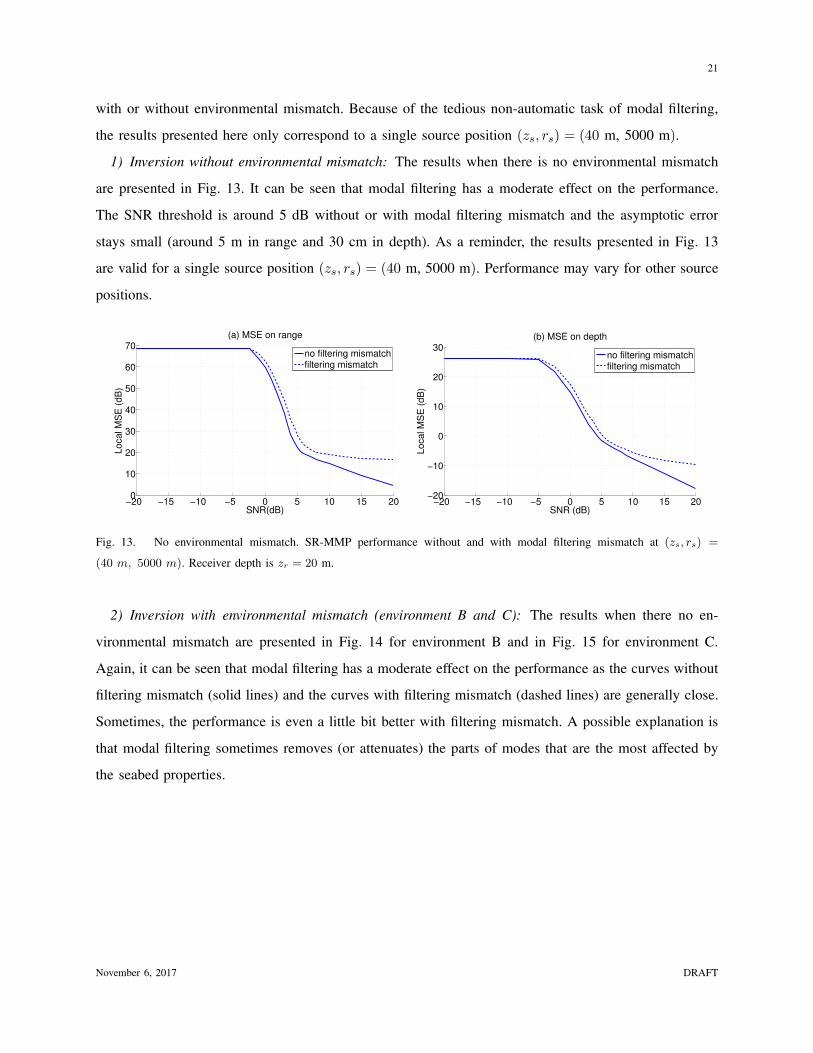
1) Inversion without environmental mismatch: The results when there is no environmental mismatch

are presented in Fig. 13. It can be seen that modal filtering has a moderate effect on the performance.

The SNR threshold is around 5 dB without or with modal filtering mismatch and the asymptotic error

stays small (around 5 m in range and 30 cm in depth). As a reminder, the results presented in Fig. 13

are valid for a single source position (zs, rs) = (40 m, 5000 m). Performance may vary for other source

positions.

−20 −15 −10 −5 0 5 10 15 200

10

20

30

40

50

60

70(a) MSE on range

Local M

SE

(dB

)

SNR(dB)

no filtering mismatchfiltering mismatch

−20 −15 −10 −5 0 5 10 15 20−20

−10

0

10

20

30(b) MSE on depth

Lo

ca

l M

SE

(d

B)

SNR (dB)

no filtering mismatchfiltering mismatch

Fig. 13. No environmental mismatch. SR-MMP performance without and with modal filtering mismatch at (zs, rs) =

(40 m, 5000 m). Receiver depth is zr = 20 m.

2) Inversion with environmental mismatch (environment B and C): The results when there no en-

vironmental mismatch are presented in Fig. 14 for environment B and in Fig. 15 for environment C.

Again, it can be seen that modal filtering has a moderate effect on the performance as the curves without

filtering mismatch (solid lines) and the curves with filtering mismatch (dashed lines) are generally close.

Sometimes, the performance is even a little bit better with filtering mismatch. A possible explanation is

that modal filtering sometimes removes (or attenuates) the parts of modes that are the most affected by

the seabed properties.


22

−20 −15 −10 −5 0 5 10 15 2010

20

30

40

50

60

70(a) MSE on range

Lo

ca

l M

SE

(d

B)

SNR(dB)

no filtering 1575 m/s

filtering 1575 m/s


filtering 1600 m/s


filtering 1625 m/s


filtering 1650 m/s

−20 −15 −10 −5 0 5 10 15 20−20

−10

0

10

20

30(b) MSE on depth

SNR (dB)

Local M

SE

(dB

)


filtering 1575 m/s


filtering 1600 m/s


filtering 1625 m/s


filtering 1650 m/s


filtering 1675 m/s

Fig. 14. Environmental mismatch B. SR-MMP performance without and with modal filtering mismatch at (zs, rs) =

(40 m, 5000 m). Receiver depth is zr = 20 m.

−20 −15 −10 −5 0 5 10 15 2030

40

50

60

70(a) MSE on range

Lo

ca

l M

SE

(d

B)

SNR(dB)


filtering 1575 m/s


filtering 1600 m/s


filtering 1625 m/s


filtering 1650 m/s


filtering 1675 m/s

−20 −15 −10 −5 0 5 10 15 20−5

0

5

10

15

20

25

30(b) MSE on depth

Lo

ca

l M

SE

(d

B)

SNR (dB)


filtering 1575 m/s


filtering 1600 m/s


filtering 1625 m/s


filtering 1650 m/s


filtering 1675 m/s

Fig. 15. Environmental mismatch C. SR-MMP performance without and with modal filtering mismatch and environmental

mismatch at (zs, rs) = (40 m, 5000 m). Receiver depth is zr = 20 m.

V. CONCLUSIONS

Single receiver matched-mode processing performances have been evaluated in typical source localiza-

tion scenarios. The SR-MMP ambiguity function exhibits a mainlobe/sidelobe behavior characteristic of

non-linear estimation problems, and the mean-square error presents three regions of operation as a function

of SNR: the high SNR asymptotic region driven by mainlobe errors, the intermediate SNR threshold region

driven by sidelobe errors and the low SNR no-information region. The method of interval errors, which

gives approximate but computationally efficient and reliable MSE performance prediction, has been used

to conduct multiple performance analyses. The performances have first been analyzed when there is no

mismatch between the assumed environment and the true environment. SR-MMP performances highly

depend on the source/receiver depth. In particular, a significant loss in performance is observed when the


23

receiver is located at a node common to two modes which shows that receiver depth must be chosen with

care. In the example studied here, an SNR of 3 dB seemed enough to obtain acceptable performance,

although this number may vary significantly in other cases (different environment, frequencies or number

of modes).

When there is mismatch between the assumed and true seabed (bottom halfspace assumed instead of

two layer bottom over bottom halfspace) performance deteriorates, the threshold region begins at higher

SNR and there is a bias at high SNR. However, it seems to remain acceptable as long as the chosen bottom

sound speed is not too far from the true bottom layers sound speeds. The results suggest that it is possible

to obtain decent performances by seeking the bottom halfspace sound-speed that best approximates the

real bottom. This would be an alternative to more complicated localization algorithms that jointly invert

over source locations and environmental parameters (e.g. [41]). When there is mismatch in both the

seabed and the water sound speed profile (constant sound speed profile instead of a thermocline), there

is a significant loss in performance. It appears that in this case, the difference between the assumed

environment and the true environment is too strong to obtain acceptable performance. Furthermore, the

impact of possible degradations resulting from non-ideal modal filtering has also been investigated: modal

filtering seems to only have a moderate impact on performance.

The analysis presented here provides a better understanding of SR-MMP and its achievable perfor-

mance. It therefore offers good prospects for future application of SR-MMP. Furthermore, while the

influence of mismatch on performances have been analyzed, another prospect could be to develop methods

for improving the robustness of SR-MMP to environmental mismatch. A possible approach would be to

adapt ideas implemented for MFP [42]–[44].

VI. ACKNOWLEDGEMENT

This work was funded by the French Government Defence procurement agency (Direction Generale

de l’Armement). JB also acknowledges the Investment in Science Fund at WHOI.

APPENDIX A

PAIRWISE ERROR PROBABILITY

The pairwise error probability Pe(θn|θm) of the ML estimator (under a possible model mismatch) is

given by

Pe(θn|θm) = P

(

K∑

k=1

|xHǫ (fk,θn)y(fk)|

2 − |xHǫ (fk,θm)y(fk)|

2

σ2w(fk)

≥ 0

)

. (13)


24

Following the same approach as in [33, Sec. III-A], this pairwise error probability can be expressed as

Pe(θn|θm) = 1−1

2π

∫ ∞

−∞

1

jω + β×

e−c

∏Kk=1(1 + λ1k

(jω + β))(1 + λ2k(jω + β))

dω, (14)

c =

K∑

k=1

λ1k|µ1k

|2(jω + β)

(1 + λ1k(jω + β))

+λ2k

|µ2k|2(jω + β)

(1 + λ2k(jω + β))

, (15)

for some β > 0 such that 1 + βλ1k> 0 and 1 + βλ2k

> 0. λ1k,2kare the non-zero eigenvalues of

xǫ(fk,θn)xǫH(fk,θn)− xǫ(fk,θm)xǫ

H(fk,θm) (16)

and satisfy

λ1k,2k= ±

√

1− |xǫH(fk,θn)xǫ(fk,θm)|. (17)

The values µ1k, µ2k

can be expressed as a function of the SNR γ(fk). In the general case with possible

mismatch they satisfy

µ1k,2k=

√

γ(fk)(1− λ1k,2k)

2λ21k,2k

×

(

xǫH(fk,θm)x(fk,θ0)−

1

1− λ1k,2k

×

xǫH(fk,θm)xǫ(fk,θn)xǫ

H(fk,θn)x(fk,θ0)

)

. (18)

APPENDIX B

ASYMPTOTIC MSE

When expanded, the MSE can be expressed as

Ey

{

(

θ − θ0

)(

θ − θ0

)T}

= Ey

{

∆θ∆θT}

+ Ey

{

∆θ

}

bT (θ0) + b(θ0)Ey

{

∆θ

}T

+ b(θ0)bT (θ0),

(19)

where ∆θ = θ − θm and b(θ0) = θm − θ0. The value θm as well as the bias b(θ0) can easily be

obtained by analyzing the AF. The asymptotic local MSE is then derived by computing an asymptotic

approximation of Ey

{

∆θ∆θT}

and Ey

{

∆θ

}

. Based on [33, Sec. III-B], we obtain the following

results. Define

ak = xǫ(fk,θm), ck = x(fk,θ0), Dk =∂xǫ(fk,θm)

∂θT, (20)

and the M ×M matrix

[F]i,j =

K∑

k=1

|s(fk)|2

σ2w(fk)

Re

[(

∂2ak∂θj∂θi

)H

ckcHk ak +

(

∂ak∂θi

)H

ckcHk

(

∂ak∂θj

)]

. (21)


25

We then obtain

Ey

{

∆θ

}

= −F−1Re

[

K∑

k=1

DHk ak

]

, (22)

and

Ey

{

∆θ∆θT}

=1

2F−1Re

[ K∑

k=1

(

DHk Dk +DH

k akaTkD

∗k

)

+|s(fk)|

2

σ2w(fk)

(

DHk ckc

Hk Dk +DH

k ckcHk aka

TkD

∗k +DH

k DkaHk ckc

Hk ak +DH

k akcTkD

∗kc

Hk ak

)

]

F−1

+ Ey

{

∆θ

}

Ey

{

∆θ

}T

.

(23)

REFERENCES

[1] A.B. Baggeroer, W.A. Kuperman, and P.N. Mikhalevsky, “An overview of matched field methods in ocean acoustics,”

IEEE Journal of Oceanic Engineering, vol. 18, no. 4, pp. 401–424, 1993.

[2] F.B. Jensen, W.A. Kuperman, and B. Michael, Computational ocean acoustics, American Institute of Physics, New York,

1994.

[3] R.G. Baraniuk and D.L. Jones, “Unitary equivalence: A new twist on signal processing,” IEEE Transactions on Signal

Processing, vol. 43, no. 10, pp. 2269–2282, 1995.

[4] G. Le Touze, B. Nicolas, J. Mars, and J.L. Lacoume, “Matched representations and filters for guided waves,” IEEE

Transactions on Signal Processing, vol. 57, no. 5, pp. 1783–1795, 2009.

[5] J. Bonnel, C. Gervaise, P. Roux, B. Nicolas, and JI Mars, “Modal depth function estimation using time-frequency analysis,”

The Journal of the Acoustical Society of America, vol. 130, pp. 61–71, 2011.

[6] J. Bonnel, G. Le Touze, B. Nicolas, and J. Mars, “Physics-based time-frequency representations for underwater acoustics:

Power class utilization with waveguide-invariant approximation,” IEEE Signal Processing Magazine, vol. 30, no. 6, pp.

120–129, 2013.

[7] J. Bonnel, A. M. Thode, S. B. Blackwell, K. Kim, and A M. Macrander, “Range estimation of bowhead whale (balaena

mysticetus) calls in the arctic using a single hydrophonea,” The Journal of the Acoustical Society of America, vol. 136,

no. 1, pp. 145–155, 2014.

[8] A. Thode, J. Bonnel, M. Thieury, A. Fagan, C. Verlinden, D. Wright, C. Berchok, and J. Crance, “Using nonlinear time

warping to estimate north pacific right whale calling depths in the bering sea,” The Journal of the Acoustical Society of

America, vol. 141, no. 5, pp. 3059–3069, 2017.

[9] G.R. Wilson, R.A. Koch, and P.J. Vidmar, “Matched mode localization,” The Journal of the Acoustical Society of America,

vol. 84, no. 1, pp. 310–320, 1988.

[10] T.C. Yang, “Effectiveness of mode filtering: A comparison of matched-field and matched-mode processing,” The Journal

of the Acoustical Society of America, vol. 87, no. 5, pp. 2072–2084, 1990.

[11] C.W. Bogart and T.C. Yang, “Comparative performance of matched-mode and matched-field localization in a range-

dependent environment,” The Journal of the Acoustical Society of America, vol. 92, pp. 2051, 1992.

[12] N.E. Collison and S.E. Dosso, “Regularized matched-mode processing,” The Journal of the Acoustical Society of America,

vol. 103, pp. 2821, 1998.


26

[13] T.B. Neilsen and E.K. Westwood, “Extraction of acoustic normal mode depth functions using vertical line array data,”

The Journal of the Acoustical Society of America, vol. 111, pp. 748–756, 2002.

[14] K. Yoo and T.C. Yang, “Broadband source localization in shallow water in the presence of internal waves,” The journal

of the Acoustical Society of America, vol. 106, no. 6, pp. 3255–3269, 1999.

[15] G. R Potty, J. H Miller, J. F Lynch, and K. B Smith, “Tomographic inversion for sediment parameters in shallow water,”

The Journal of the Acoustical Society of America, vol. 108, no. 3, pp. 973–986, 2000.

[16] S.D. Rajan and K.M. Becker, “Inversion for range-dependent sediment compressional-wave-speed profiles from modal

dispersion data,” IEEE Journal of Oceanic Engineering, vol. 35, no. 1, pp. 43–58, 2010.

[17] J. Bonnel, S. E Dosso, and N R. Chapman, “Bayesian geoacoustic inversion of single hydrophone light bulb data using

warping dispersion analysis,” The Journal of the Acoustical Society of America, vol. 134, no. 1, pp. 120–130, 2013.

[18] L. Wan, J.X. Zhou, and P.H. Rogers, “Low-frequency sound speed and attenuation in sandy seabottom from long-range

broadband acoustic measurements,” The Journal of the Acoustical Society of America, vol. 128, no. 2, pp. 578–589, 2010.

[19] J. Zeng, N R. Chapman, and J. Bonnel, “Inversion of seabed attenuation using time-warping of close range data,” The

Journal of the Acoustical Society of America, vol. 134, no. 5, pp. EL394–EL399, 2013.

[20] G. Le Touze, J. Torras, B. Nicolas, and Jerome Mars, “Source localization on a single hydrophone,” in OCEANS. IEEE,

2008, pp. 1–6.

[21] G. Le Touze, Localisation de source par petits fonds en UBF (1-100 Hz) a l’aide d’outils temps-frequence, Ph.D. thesis,

Institut National Polytechnique de Grenoble, 2007.

[22] B. Nicolas, G. Le Touze, C. Soares, S. Jesus, and JI Marsal, “Incoherent versus coherent matched mode processing for

shallow water source localisation using a single hydrophone,” Instrumentation viewpoint, vol. 8, pp. 67–68, 2009.

[23] J. Bonnel and A. Thode, “Range and depth estimation of bowhead whale calls in the arctic using a single hydrophone,”

in Sensor Systems for a Changing Ocean (SSCO). IEEE, 2014, pp. 1–4.

[24] Harry L Van Trees, Detection, Estimation, and Linear Modulation Theory, Part I, Wiley, New York, 1968.

[25] C.D. Richmond, “Mean-squared error and threshold snr prediction of maximum-likelihood signal parameter estimation

with estimated colored noise covariances,” IEEE Transactions on Information Theory, vol. 52, no. 5, pp. 2146–2164, 2006.

[26] A.B. Baggeroer and H. Schmidt, “Cramer-rao bounds for matched field tomography and ocean acoustic tomography,” in

International Conference on Acoustics, Speech and Signal Processing (ICASSP). IEEE, 1995, vol. 5, pp. 2763–2766.

[27] J. Tabrikian and J.L. Krolik, “Barankin bounds for source localization in an uncertain ocean environment,” IEEE


[28] W. Xu, A.B. Baggeroer, and C.D. Richmond, “Bayesian bounds for matched-field parameter estimation,” IEEE Transactions

on Signal Processing, vol. 52, no. 12, pp. 3293–3305, 2004.

[29] Wen Xu, Arthur B Baggeroer, and Henrik Schmidt, “Performance analysis for matched-field source localization: Simulations

and experimental results,” IEEE Journal of Oceanic Engineering, vol. 31, no. 2, pp. 325–344, 2006.

[30] W. Xu, Z. Xiao, and L. Yu, “Performance analysis of matched-field source localization under spatially correlated noise

field,” IEEE Journal of Oceanic Engineering, vol. 36, no. 2, pp. 273–284, 2011.

[31] Y. Le Gall, F.-X. Socheleau, and J. Bonnel, “Performance analysis of single receiver matched-mode processing for source

localization,” in 2nd Underwater Acoustics Conference and Exhibition (UA2014), 2014.

[32] Y. Le Gall, F.-X. Socheleau, and J. Bonnel, “Matched-Field Processing Performance Under the Stochastic and Deterministic

Signal Models,” IEEE Transactions on Signal Processing, vol. 62, no. 22, pp. 5825–5838, 2014.


27

[33] Y. Le Gall, F.-X. Socheleau, and J. Bonnel, “Matched-Field Performance Prediction with Model Mismatch,” IEEE Signal

Processing Letters, vol. 23, no. 4, pp. 409 – 413, 2016.

[34] C.F. Mecklenbrauker and P. Gerstoft, “Objective functions for ocean acoustic inversion derived by likelihood methods,”

Journal of Computational Acoustics, vol. 8, no. 02, pp. 259–270, 2000.

[35] S. E Dosso and M. J. Wilmut, “Maximum-likelihood and other processors for incoherent and coherent matched-field

localization,” The Journal of the Acoustical Society of America, vol. 132, no. 4, pp. 2273–2285, 2012.

[36] Y. Pawitan, In all likelihood: statistical modelling and inference using likelihood, Oxford University Press, 2001.

[37] H.L. Van Trees and K.L. Bell, Bayesian bounds for parameter estimation and nonlinear filtering/tracking, Wiley-IEEE

Press, 2007.

[38] C. D. Richmond, “Capon algorithm mean-squared error threshold snr prediction and probability of resolution,” IEEE


[39] C. D. Richmond, “On the threshold region mean-squared error performance of maximum-likelihood direction-of arrival

estimation in the presence of signal model mismatch,” in Workshop on Sensor Array and Multichannel Processing. IEEE,

2006, pp. 268–272.

[40] F. Athley, “Threshold region performance of maximum likelihood direction of arrival estimators,” IEEE Transactions on

Signal Processing, vol. 53, no. 4, pp. 1359–1373, 2005.

[41] S. E. Dosso and M. J. Wilmut, “Comparison of focalization and marginalization for bayesian tracking in an uncertain

ocean environment,” The Journal of the Acoustical Society of America, vol. 125, no. 2, pp. 717–722, 2009.

[42] J.L. Krolik, “Matched-field minimum variance beamforming in a random ocean channel,” The Journal of the Acoustical

Society of America, vol. 92, no. 3, pp. 1408–1419, 1992.

[43] J. Tabrikian, J.L. Krolik, and H. Messer, “Robust maximum-likelihood source localization in an uncertain shallow-water

waveguide,” The Journal of the Acoustical Society of America, vol. 101, no. 1, pp. 241–249, 1997.

[44] Y. Le Gall, S. E Dosso, F.-X. Socheleau, and J. Bonnel, “Bayesian source localization with uncertain green’s function in

an uncertain shallow water ocean,” The Journal of the Acoustical Society of America, vol. 139, no. 3, pp. 993 – 1004,

2016.

PLACE

PHOTO

HERE

Yann Le Gall (S’12) received the Dipl.Ing. degree in signal processing from Grenoble Institut National

Polytechnique (Grenoble INP), Grenoble, France, in 2012, and the Ph.D. degree in signal processing at

Lab-STICC (UMR 6285), ENSTA Bretagne, Brest, France in 2015. He is currently a research engineer

at Thales Underwater Systems, Brest, France. His research interests in the field of signal processing

and underwater acoustics include source detection/localization, geoacoustic inversion and performance

prediction.


28

PLACE

PHOTO

HERE

Francois-Xavier Socheleau (S’08-M’12) graduated in electrical engineering from ESEO, Angers, France,

in 2001 and received the Ph.D. degree from Telecom Bretagne, Brest, France, in 2011.

From 2001 to 2004, he was a Research Engineer at Thales Communications, France, where he worked on

electronic warfare systems. From 2005 to 2007, he was employed at Navman Wireless (New Zealand/U.K.)

as an R&D Engineer. From 2008 to 2011, he worked for Thales Underwater Systems, France. In November

2011, he joined ENSTA Bretagne as an Assistant Professor. Since September 2014, he has been an

Associate Professor at IMT Atlantique (formerly known as Telecom Bretagne), France. His research interests include signal

processing, wireless communications and underwater acoustics.

PLACE

PHOTO

HERE

Julien Bonnel (S’08 - M’11) received the Ph.D. degree in signal processing from Grenoble Institut

National Polytechnique (Grenoble INP), Grenoble, France, in 2010.

From 2010 to 2017, he was an Assistant Professor at Lab-STICC (UMR 6285), ENSTA Bretagne in

Brest, France. Since September 2017, he has been an Associate Scientist at Woods Hole Oceanographic

Institution, USA. His research in signal processing and underwater acoustics include time-frequency

analysis, source detection/localization, geoacoustic inversion, acoustical tomography, passive acoustic

monitoring, and bioacoustics. He is a Member of the Acoustical Society of America.


1 performance analysis of single receiver matched-mode

Documents