1 linear immigration-death models - home - dept. of ...twehrly/664/chapter3.pdf · • consider the...

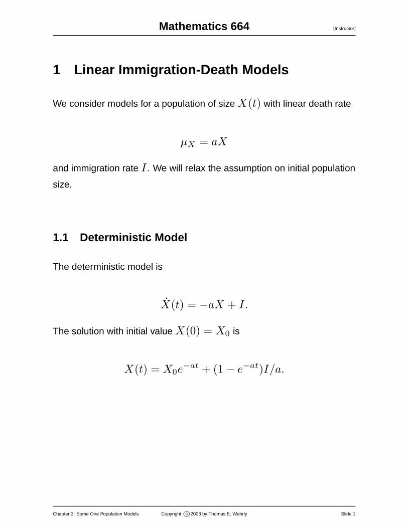
Mathematics 664 [Instructor]

1 Linear Immigration-Death Models

We consider models for a population of size X(t) with linear death rate

µX = aX

and immigration rate I . We will relax the assumption on initial population

size.

1.1 Deterministic Model

The deterministic model is

X(t) = −aX + I.

The solution with initial value X(0) = X0 is

X(t) = X0e−at + (1− e−at)I/a.

Chapter 3: Some One Population Models Copyright c©2003 by Thomas E. Wehrly Slide 1


Example: Let X(t) = the number of Africanized honey bee (AHB)

colonies at time t in a given region. Suppose the following assumed

parameters:

I = 1.4 colonies/time

a = 0.08 (time−1)

X(0) = 2 colonies

The deterministic solution is

X(t) = 17.5− 15.5e−0.08t.

0 10 20 30 40 50 60

05

1015

20

time

num

ber

of c

olon

ies



1.2 Stochastic Model

Earlier we found the PDE for the pgf

∂P (s, t)∂t

= I(s− 1)P (s, t) + a(1− s)∂P (s, t)

∂s

The solution corresponding to X(0) = X0 is

P (s, t) = [1 + (s− 1)e−at]X0 exp{(s− 1)(1− e−at)I/a}

The pgf (or mgf) can be used to determine various properties of the

probability distribution of X(t).

• Consider the limiting distribution of the equilibrium population size

X∗ as t →∞. Since a > 0, the pgf of X∗ is

P (s,∞) = exp{(s− 1)I/a}.

This is the pgf of the Poisson distribution with parameter λ = I/a.

The limiting distribution is independent of the initial population size,

X0.



• Note that the pgf is the product of two factors.

– The first factor is the pgf of a binomial distribution with n = X0

and p = e−at.

– The second factor is the pgf of a Poisson distribution with

parameter λ = (1− e−at)I/a.

• This implies that we can write

X(t) = X1(t) + X2(t)

where X1(t) and X2(t) are independent random variables with the

above binomial and Poisson distributions, respectively.

• The moment generating function is

M(θ, t) = P (eθ, t)

The cumulant generating function then is

K(θ, t) = (eθ − 1)(1− e−at)I/a + X0 log[1 + (eθ − 1)e−at]

The first three cumulants are

µ(t) = X0e−at + (1− e−at)I/a

σ2(t) = µ(t)−X0e−2at

κ3(t) = σ2(t)− 2X0e−2at(1− e−at)



1.3 Application to the AHB Population Dynamics

We return to the AHB population dynamics example with

I = 1.4 colonies/time

a = 0.08 (time−1)

X(0) = 2 colonies

The deterministic solution is

X(t) = 17.5− 15.5e−0.08t.

• The equilibrium solution is X∗ = 17.5. For the stochastic model,

the equilibrium solution X∗ is now a Poisson random variable with

parameter I/a = 17.5. The probability distribution and its

saddlepoint approximation appear in the figure:

5 6 7 8 9 101112131415161718192021222324252627282930

0.0

0.02

0.04

0.06

0.08



• The transient probability distributions are also of interest. They could

be obtained directly from the pgf or mgf. To illustrate the variation in

the AHB model, we will simulate the process several times using the

assumed parameters. Notice the large amount of variation about the

mean function.

Simulations of AHB Population Dynamics

time

colo

nies

0 20 40 60

05

1015

2025



• Several more sample paths with the same parameter values:

time

sp

0 20 40 60 80

510

1520

time

sp

0 20 40 60 80

510

1520

2530

time

sp

0 20 40 60 80

510

1520

25

time

sp

0 20 40 60 80

510

1520

time

sp

0 20 40 60 80

510

1520

time

sp

0 20 40 60

510

1520

time

sp

0 20 40 60

510

1520

25

time

sp

0 20 40 60

510

1520



2 Linear Birth-Immigration-Death Models

We now consider a process that has a linear birth rate in addition to the

linear death rate:

λX = a1X and µX = a2X

The immigration rate is assumed to equal I .

2.1 Solution to the Deterministic Model

The deterministic model can be written as

X(t) = aX(t) + I where a = a1 − a2.

The solution is

X(t) = X0eat + (eat − 1)I/a.

If a < 0, the equilibrium value is−I/a.



2.2 Probability Distributions for the Stochastic Model

The Kolmogorov forward equations are

px(t) = [I+a1(x−1)]px−1(t)−[I+(a1+a2)x]px(t)+a2(x+1)px+1(t)

for x > 0 and

p0(t) = −Ip0(t) + a2p1(t)

The R matrix is tridiagonal with elements

ri,j =

ri,i+1 = I + ia1

ri,i−1 = ia2

ri,i = −I − i(a1 + a2)

ri,j = 0 for |i− j| > 1.

The equilibrium distribution can be derived from the Kolmogorov

equations by setting p(t) = 0. Letting πi = pi(∞), we get

π1 = π0(I/a1)

π2 = π0I(I + a1)/2a22

......

πi = π0(a1/a2)i(i−1+(I/a1)

i

)



If a1 < a2, we can solve for π0 by summing:

π0 = (−a/a2)i/a1

We find that the distribution of X∗ is the negative binomial distribution

with pmf

πi =(

k − 1 + i

i

)pk(1− p)i

where k = I/a1 and p = −a/a2.

2.3 Generating Functions

The intensity functions are

f1 = I + a1x and f−1 = a2x.

The resulting PDE is

∂P

∂t= I(s− 1)P (s, t) + [a1s(1− s) + a2(1− s)∂P (s, t)/∂s.

The analytical solution is

P (s, t) =aI/a1{a2(eat − 1)− (a2e

at − a1)s}X0

{(a1eat − a2)− a1s(eat − 1)}X0+I/a1

It would be difficult to solve for the transition probabilities by successive

differentiation. However,

p0(t) = P (0, t) = aI/a1(a2eat − a2)X0(a1e

at = a2)−X0−I/a1 .



The cumulant generating function is given by

∂K

∂t= I(eθ − 1) +

{a1(e−θ − 1) + a2(e−θ − 1)

} ∂K

∂θ.

Using a series expansion, we obtain ODEs for the first three cumulants:

κ1(t) = I + aκ1

κ2(t) = I + cκ1 + 2aκ2

κ3(t) = I + aκ1 + 3cκ2 + 3aκ3

These can be solved recursively when X(0) = X0:

κ1(t) = X0eat + (eat − 1)I/a

κ2(t) = X0ceat(eat − 1)/a + I(eat − 1)(a1e

at − a2)/a2

κ3(t) = X0eat

[3c2(eat − 1)2 + a2(e2at − 1)

]/2a2

+[−2ca2 + (3c2 − a2)eat − 6a1ce

2at + 4a21e

3at]/2a3



2.4 Application to AHB

Consider the linear birth-death-immigration model with parameters;

I = 1.4 a1 = 0.08

X(0) = 2 a2 = 0.16

Since the negative net growth rate is a = −0.08, the solution to the

deterministic model is the same as the linear death-immigration process

with the same death rate.

However, there is a large difference between the stochastic models in

the two situations. We saw earlier that the equilibrium distribution of X∗

was Poisson with mean 17.5 for the LID process. For the LBID model,

the equilibrium distribution is negative binomial with k = 17.5 and

p = 0.5. The LBID has much greater variance.

0 1 2 3 4 5 6 7 8 910111213141516171819202122232425262728293031323334353637383940

0.0

0.02

0.04

0.06



Variance Functions for LID and LBID Models

time

varia

nce

0 10 20 30 40 50 60

010

2030

40

LID ModeLBID Model

2.5 Simulation of the LBID Process

• The times between arrivals due to immigration will have an

exponential distribution with parameter I (mean 1/I).

• The times until the next death or birth will have an exponential

distribution with parameter µX = aX(t) where a = a1 + a2.

• The next event will be a birth with probability a1/a and a death with

probability a2/a.



• The algorithm for simulation the process can be summarized as

follows:

1. Set X(0) = X0.

2. If X(ti) = 0, generate tI from exp(I) distribution. Set

ti = ti−1 + tI and X(ti) = 1.

3. Otherwise, generate tI from exp(I) distribution and tD from

exp(aX(ti)) distribution.

(a) If tI < tD set ti = ti−1 + tI and X(ti) = X(ti−1) + 1.

(b) If tI > tD , generate U = a uniform(0,1) variable.

i. If U < a1/a set ti = ti−1 + tD and

X(ti) = X(ti−1) + 1.

ii. If U > a1/a, set ti = ti−1 + tD and

X(ti) = X(ti−1)− 1.

4. Return to Step 3.Several Realizations of LBID Process

time

x(t)

0 5 10 15 20 25

05

1015

2025



• Several More Realizations with the Same Parameter Values:

time

sp

0 5 10 15

510

1520

2530

time

sp

0 5 10 15 20 25 30

24

68

1012

14

time

sp

0 5 10 15 20 25 30

510

15

time

sp

0 5 10 15 20 25

510

1520

time

sp

0 5 10 15 20 25

510

15

time

sp

0 5 10 15 20

510

15

time

sp

0 5 10 15 20 25

510

1520

25

time

sp

0 5 10 15 20 25

510

1520



3 Nonlinear Birth–Death Models

We now look at population models with nonlinear death rates. Consider

the model with population rates

λX =

a1X − b1Xs+1 for X < (a1/b1)1/s

0 otherwise

µX = a2X + b2Xs+1

We call a1, a2 the intrinsic rates, and b1, b2 are the crowding

coefficients that add density dependence to the model. We will look at

the special case with s = 1 which leads to the logistic model.


We can write the deterministic model as

X(t) = aX − bXs+1

where a = a1− a2 and b = b1 − b2. This has solution

X(t) =K

[1 + m exp(−ast)]1/s

with

K = (a/b)1/s and m = (K/K0)s − 1



3.2 Probability Distributions for the Stochastic Model

Assume that u = (a1/b1)1/s be an integer. We can obtain the system

of u + 1 Kolmogorov differential equations for the probabilities:

p0(t) = µ1p1(t)

p1(t) = −(λ1 + µ1)p1(t) + µ2(t)p2(t)

px(t) = λx−1px−1(t)− (λx + µx)px(t) + µx+1px+1(t),

for x = 2, . . . , u− 1

pu(t) = λu−1pu−1(t)− µupu(t)

• Since there are only a finite number of equations, one can obtain

numerical solutions.

• Since u is finite, the a population size of 0 is an absorbing state and

ultimate extinction is certain, i.e., p0(∞) = 1.

• A process is said to be ecologically stable if the extinction does not

occur within a realizable time interval. A quantity of interest is the

expected time until extinction, Ex.

• The quasi-equilibrium distribution is based on the idea that the

population in equilibrium would not drift. The probabilities would

satisfy the relationship



µxpx(t) = λx−1px−1(t) for x = 2, . . . , u

3.3 Generating Functions and Cumulants

The intensity functions are

f1 = a1x− b1xs+1

f−1 = a2x + b2xs+1

The PDE for the pgf has the form

∂P

∂t= (s− 1)(a1s− a2)∂P (s, t)/∂s + s(s− 1)(b1s + b2)

∂2P

∂s2.

This equation is analytically intractible. By substituting eθ for s we get

the PDE for the mgf, M(θ, t). Letting K log M , we obtain the equation

for the cgf:

∂K∂t =

[(eθ − 1)a1 + (e−θ − 1)a2

]∂K∂θ

+[(eθ − 1)(−b1) + (e−θ − 1)b2

] [∂2K∂θ2 +

(∂K∂θ

)2]

Again, we can obtain differential equations for the cumulants. For s = 1,

the first cumulant is

κ1(t) = (a− bκ1)κ1 − bκ2



• The differential equation for the jth cumulant depends on cumulants

up to order j + s. This rules out finding exact solutions.

• One proposed approach is to set all cumulants above a certain order

equal to zero and then solve the resulting finite system.

3.4 Application to AHB Population Dynamics

The nonlinear birth-death model with similar mean properties to the

earlier models for AHB population dynamics has parameter values:

a1 = 0.30 a2 = 0.02

b1 = 0.015 b2 = 0.001.

The solution to the deterministic model is

X(t) =17.5

1 + 7.75e−0.28t.

Deterministic Solution of NLBD Model

Time

X(t

)

0 20 40 60 80 100

510

15



• Simulation of the NLBD Model

1. Compute the birth and death rates: b(x) = a1x− b1x2 for

x < (a1/b1)1/s and d(x) = a2x + b2x2.

2. Compute the time to the next event as exponential(a(x) + b(x))

random variable.

3. Generate a uniform(0,1) random variable U . If

U < a(x)/(a(x) + b(x)), then the next event is a birth.

Otherwise, it is a death.

• Some realizations of the NLBD model:

Some Realizations of the NLBD Model

Time

X(t

)

0 20 40 60 80 100

05

1015

2025



4 Nonlinear Birth-Immigration-Death Models

In addition to the assumptions of nonlinear birth and death rates, we

assume that there is a constant immigration rate I .


The deterministic model is

X(t) = I + aX − bXs+1

where a = a1− a2 and b = b1 − b2. This has solution for s = 1:

X(t) ={

a + β

[1− δe−βt

1 + δe−βt

]}/2b

where

β = (a2 + 4bI)1/2

γ = (2bX0 − a)/β

δ = (1− γ)/(1 + γ)

The carrying capacity is

K = (a + β)/2b



4.2 Simulation of the Stochastic Model

• The analysis of the stochastic model can be carried out by

numerically solving the differential equations for the cumulatants.

• However, the simulation of this model is still quite simple.

• Replace the birth rate in the simulation procedure for the NLBD

model with b(x) = I + a1x− b1x2. Steps 2 and 3 are the same

as before. The one care that needs to be taken is to check whether

the value of X(t) is above the carrying capacity.

4.3 Application to AHB Population Dynamics

The paramater values for the NLBID model keeping the same carrying

capacity as before are:

a1 = 0.30 a2 = 0.02

b1 = 0.012 b2 = 0.004816.

I = 0.25.

The solution to the deterministic model with X(0) = 2 is

X(t) = 8.3254 + 0.1749[1− δe−βt

1 + δe−βt

]

where δ = 5.4364 and β = 0.308571.


1 linear immigration-death models - home - dept. of ...twehrly/664/chapter3.pdf · • consider the...

Documents