1 introduction to approximation algorithms lecture 15: mar 5
Post on 22-Dec-2015
215 views
TRANSCRIPT

1
Introduction to
Approximation
Algorithms
Lecture 15: Mar 5

2
NP-completeness
Do your best then.

3
Different Approaches
Special graph classes
e.g. vertex cover in bipartite graphs, perfect graphs.
Fast exact algorithms, fixed parameter algorithms
find a vertex cover of size k efficiently for small k.
Average case analysis
find an algorithm which works well on average.
Approximation algorithms
find an algorithm which return solutions that are
guaranteed to be close to an optimal solution.

4
Vertex Cover
Vertex cover: a subset of vertices which “covers” every edge.
An edge is covered if one of its endpoint is chosen.
The Minimum Vertex Cover Problem:
Find a vertex cover with minimum number of vertices.

5
Approximation Algorithms
Constant factor approximation algorithms:
SOL <= cOPT for some constant c.
Key: provably close to optimal.
Let OPT be the value of an optimal solution,
and let SOL be the value of the solution that our algorithm returned.

6
Vertex Cover: Greedy Algorithm 1
Idea: Keep finding a vertex which covers the maximum number of edges.
Greedy Algorithm 1:
1. Find a vertex v with maximum degree.
2. Add v to the solution and remove v and all its incident edges from the graph.
3. Repeat until all the edges are covered.
How good is this algorithm?

7
Vertex Cover: Greedy Algorithm 1
OPT = 6, all red vertices.
SOL = 11, if we are unlucky in breaking ties.
First we might choose all the green vertices.
Then we might choose all the blue vertices.
And then we might choose all the orange vertices.

8
Vertex Cover: Greedy Algorithm 1
k! vertices of degree k
Generalizingthe example!
k!/k vertices of degree k k!/(k-1) vertices of degree k-1 k! vertices of degree 1
OPT = k!, all top vertices.
SOL = k! (1/k + 1/(k-1) + 1/(k-2) + … + 1) ≈ k! log(k), all bottom vertices.
Not a constant factor approximation algorithm!

9
Vertex Cover: Greedy Algorithm 2
In bipartite graphs, maximum matching = minimum vertex cover.
In general graphs, this is not true.
How large can this gap be?

10
Vertex Cover: Greedy Algorithm 2
Fix a maximum matching. Call the vertices involved black.
Since the matching is maximum, every edge must have a black endpoint.
So, by choosing all the black vertices, we have a vertex cover.
SOL <= 2 * size of a maximum matching

11
Vertex Cover: Greedy Algorithm 2
What about an optimal solution?
Each edge in the matching has to be covered by a different vertex!
OPT >= size of a maximum matching
So, OPT <= 2 SOL, and we have a 2-approximation algorithm!
12
Vertex Cover
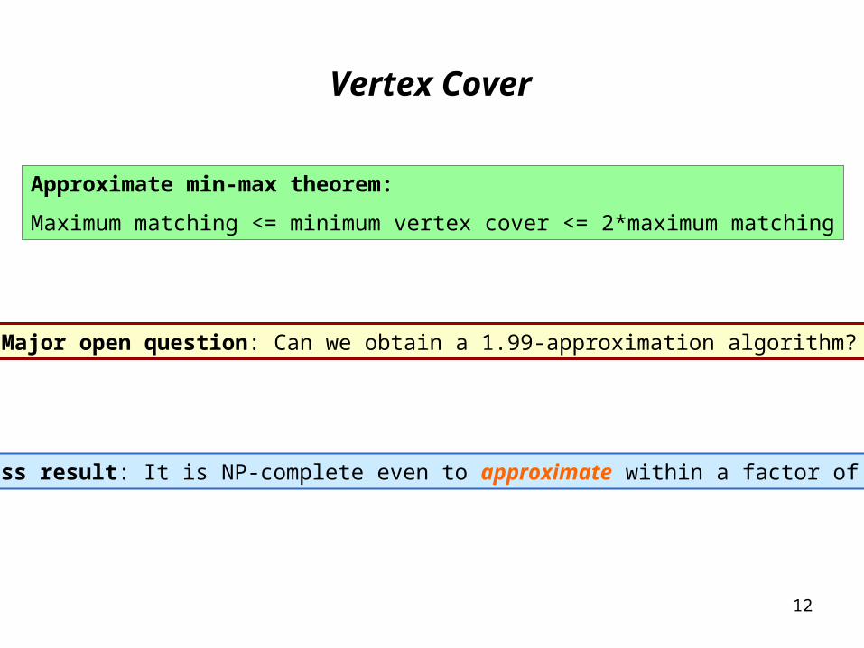
Major open question: Can we obtain a 1.99-approximation algorithm?
Hardness result: It is NP-complete even to approximate within a factor of 1.36!
Approximate min-max theorem:
Maximum matching <= minimum vertex cover <= 2*maximum matching

13
Set Cover
Set cover problem:
Given a ground set U of n elements, a collection of subsets of U,
S* = {S1,S2,…,Sk}, where each subset has a cost c(Si),
find a minimum cost subcollection of S* that covers all elements of U.
Vertex cover is a special case, why?
A convenient interpretation:
sets
elements
Choose a min-cost set of white vertices to “cover” all black vertices.

14
Greedy Algorithm
Idea: Keep finding a set which is the most effective in covering remaining elements.
Greedy Algorithm:
1. Find a set S which is most cost-effective.
2. Add S to the solution and remove all the elements it covered from the ground set.
3. Repeat until all the elements are covered.
How good is this algorithm?

15
Logarithmic Approximation
Theorem. The greedy algorithm is an O(log n) approximation for the set cover problem.
Theorem. Unless P=NP, there is no o(log n) approximation for set cover!
16
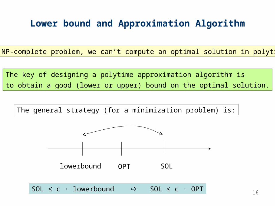
Lower bound and Approximation Algorithm
The key of designing a polytime approximation algorithm is to obtain a good (lower or upper) bound on the optimal solution.
For NP-complete problem, we can’t compute an optimal solution in polytime.
The general strategy (for a minimization problem) is:
lowerbound OPT SOL
SOL ≤ c · lowerbound SOL ≤ c · OPT

17
Linear Programming and Approximation Algorithm
lowerbound OPT SOL
Linear programming: a general method to compute a lowerbound in polytime.
LP
To computer an approximate solution,
we need to return an (integral) solution
close to an optimal LP (fractional) solution.

18
An Example: Vertex Cover
Integrality gap:=Optimal integer solution.
Optimal fractional solution.Over all instances.
In vertex cover, there are instances where this gap is almost 2.
max
1
1
1 1
00.5
0.5
0.5 0.5
0.5

19
Linear Programming Relaxation for Vertex Cover
Theorem: For the vertex cover problem, every vertex (or basic) solution of the LP is half-integral, i.e. x(v) = {0, ½, 1}
20
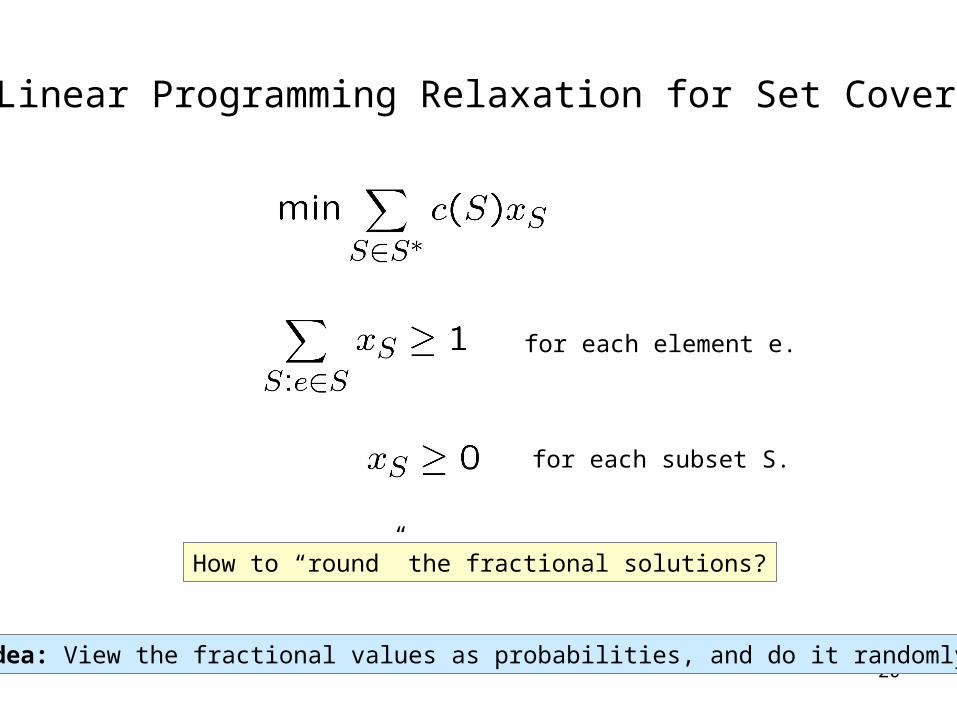
Linear Programming Relaxation for Set Cover
for each element e.
for each subset S.
How to “round” the fractional solutions?
Idea: View the fractional values as probabilities, and do it randomly!

21
sets
elements
Algorithm
First solve the linear program to obtain the fractional values x*.
0.3 0.6 0.2 0.7 0.4
Then flip a (biased) coin for each set with probability x*(S) being “head”.
Add all the “head” vertices to the set cover. Repeat log(n) rounds.

22
Performance
Theorem: The randomized rounding gives an O(log(n))-approximation.
Claim 1: The sets picked in each round have an expected cost of at most LP.
Claim 2: Each element is covered with high probability after O(log(n)) rounds.
So, after O(log(n)) rounds, the expected total cost is at most O(log(n)) LP,
and every element is covered with high probability, and hence the theorem.
Remark: It is NP-hard to have a better than O(log(n))-approximation!
23
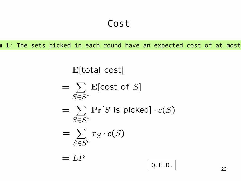
Cost
Claim 1: The sets picked in each round have an expected cost of at most LP.
Q.E.D.

24
Feasibility
First consider the probability that an element e is covered after one round.
Claim 2: Each element is covered with high probability after O(log(n)) rounds.
Let say e is covered by S1, …, Sk which have values x1, …, xk.
By the linear program, x1 + x2 + … + xk >= 1.
Pr[e is not covered in one round] = (1 – x1)(1 – x2)…(1 – xk).
This is maximized when x1=x2=…=xk=1/k, why?
Pr[e is not covered in one round] <= (1 – 1/k)k

25
Feasibility
First consider the probability that an element e is covered after one round.
Claim 2: Each element is covered with high probability after O(log(n)) rounds.
Pr[e is not covered in one round] <= (1 – 1/k)k
So,
What about after O(log(n)) rounds?

26
Feasibility
Claim 2: Each element is covered with high probability after O(log(n)) rounds.
So,
So,

27
Remark
Let say the sets picked have an expected total cost of at most clog(n) LP.
Claim: The total cost is greater than 4clog(n) LP with probability at most ¼.
This follows from the Markov inequality, which says that:
Proof of Markov inequality:
The claim follows by substituting E[X]=clog(n)LP and t=4clog(n)LP
28
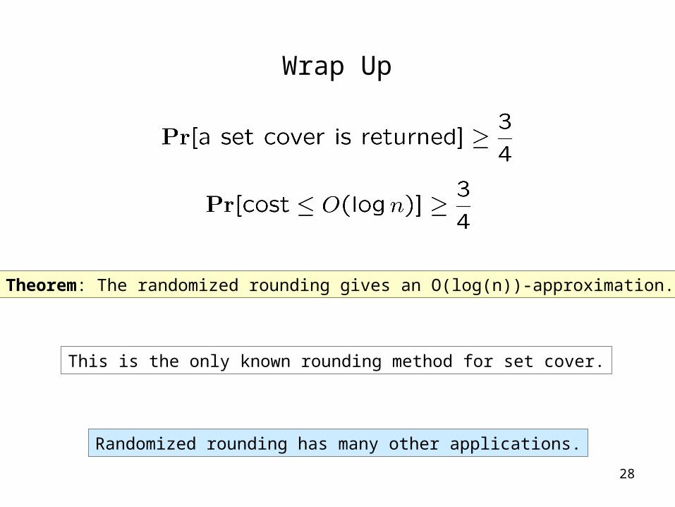
Wrap Up
Theorem: The randomized rounding gives an O(log(n))-approximation.
This is the only known rounding method for set cover.
Randomized rounding has many other applications.