approximation algorithms for re-optimization -...
TRANSCRIPT

Approximation Algorithms for Re-optimizationDRAFT – PLEASE DO NOT CITE
Dean Alderucci
Table of Contents1.Introduction ............................................................................................................................................. 22.Overview of the Current State of Re-Optimization Research ................................................................. 3
2.1.General Results for Re-optimization ............................................................................................... 32.2. Re-optimization of a General NP-hard Problem Remains NP-hard ............................................... 42.3.Hereditary Problems ........................................................................................................................ 5
2.3.1.A constant time (½)-approximation for hereditary graph problems with node insertions ....... 52.3.2.An improved approximation ratio for hereditary graph problems with node insertions ......... 62.3.3.A PTAS for certain unweighted hereditary graph problems with node insertions .................. 92.3.4.Hereditary graph problems with node deletions ...................................................................... 9
2.4.Overview of Re-optimization Results for Specific Problems ....................................................... 112.4.1.Min Coloring .......................................................................................................................... 112.4.2.Max k-Colorable Subgraph .................................................................................................... 112.4.3.Min Traveling Salesman Problem ......................................................................................... 122.4.4.Min Steiner Tree .................................................................................................................... 122.4.5.Max Knapsack ....................................................................................................................... 132.4.6.Max Weighted Independent Set ............................................................................................. 13
2.5.Some Future Directions for Re-optimization ................................................................................ 153.Some Original Results for Re-Optimization Problems ......................................................................... 16
3.1.A Generalization of Hereditary Problems ..................................................................................... 163.2.A Generalized Class of Problems for Added Components ............................................................ 17
3.2.1.Required Characteristics for Problems in this Class .............................................................. 183.2.2.A constant time (½)-approximation for WEIGHT-ADD problems ...................................... 203.2.3.A PTAS for certain WEIGHT-ADD instances ....................................................................... 223.2.4.An improved approximation ratio for WEIGHT-ADD problems .......................................... 28
3.3.A Generalized Class of Problems for Deleted Components .......................................................... 313.3.1.Max Weighted Independent Set with Added Edges ............................................................... 32
3.4.Probabilistic Distribution of Component Weights ......................................................................... 363.5.Future Work on the Generalized Class .......................................................................................... 39
4.Bibliography .......................................................................................................................................... 40Appendix A: Hereditary Graph Problems are a subclass of WEIGHT-ADD .......................................... 42Appendix B: Meeting Characteristic E for a Max Weighted k-SAT problem .......................................... 43
Page 1

1. IntroductionThis paper addresses the area of approximation with respect to re-optimization algorithms. In this classof algorithms, we are given an instance of a problem, its solution, and a local (small) modification to the instance. The objective is to solve the modified instance with the aid of the solution to the original instance.
Section 2 summarizes some of the current research in approximation algorithms for re-optimization. This includes principles of general applicability as well as results for particular NP-hard problems. A substantial part of this section deals with re-optimization of the class generally known as hereditary problems.
Section 3 presents some original algorithms related to approximation algorithms for re-optimization. These new algorithms are a generalization of existing algorithms for hereditary problems, but are applicable to a wider variety of NP-hard problems and afford better approximation ratios than those previously disclosed in the literature.
The following notation and terminology is used throughout this paper:
IOLD, INEW the original and locally-modified instance, respectivelyΔI a local change to instance II + ΔI the instance that results from making local change ΔI to I, e.g., IOLD + ΔIOLD= INEW
OPT(I) an optimal solution of instance IS, Si a solution produced by an algorithmw(x) the weight of x, e.g., of a clause in a SAT instance, of a SAT solutionk, K constants, which are independent of the size of the input under consideration
The convention in this paper is that all approximation ratios for maximization problems are expressed as values less than 1, rather than greater than 1.
References to a “conventional” problem or to a “conventional” algorithm are to emphasize that the problem or algorithm does not involve re-optimization.
For simplicity of exposition, it is assumed that P ≠ NP in all statements regarding approximability results.
Page 2

2. Overview of the Current State of Re-Optimization Research
2.1. General Results for Re-optimization
In a re-optimization problem, we are given three inputs:• an instance IOLD of a problem, • a feasible solution SOLD for that instance, and • a local (small) modification to the original instance, yielding a new instance INEW
The objective of the re-optimization problem is find an acceptable approximate solution SNEW for the new instance INEW, utilizing the information of the prior instance and solution.
In some contexts, the provided solution to the original instance is optimal.
SOLD = OPT(IOLD)
For some time, re-optimization has been studied in the context of polynomial time solvable optimization problems. For example, maintaining the optimal solution for minimum spanning tree [F] and shortest path [EG] problems under various types of local changes to the problem instance.
In contrast to problems which can be solved in polynomial time, the benefit that re-optimization confers in solving an NP-hard optimization problem depends intimately on the particular problem. As described in the next section, the re-optimization framework does not help solve NP-hard problems exactly. However, for many classes of problems, re-optimization improves the approximability, sometimes significantly, when compared to the approximation algorithm for the corresponding conventional problem.
Re-optimization may provide an improvement in the time required to solve the problem and / or in approximability of the problem. For example, utilizing the original solution may yield a better constant approximation ratio (e.g., as in metric TSP where one edge's cost is changed), or may admit a PTAS where one does not exist for the conventional problem (e.g., as in certain classes of Steiner tree where the number of terminal nodes is changed). On the other hand, there are many problems (e.g., general TSP where one edge's cost is changed) for which utilizing a solution to a similar problem provides no advantage whatsoever in approximability.
For some problems, it is obvious how to exploit the previous solution, because an optimal solution or a good approximation for the original instance is itself a close approximation for the modified instance. This is especially true if the local change is 'small'. For example, adding a single edge to an instance of a graph coloring problem can increase the optimal solution by at most one, which may be an acceptableapproximation in some contexts, though in other contexts it will clearly not be.
Page 3

2.2. Re-optimization of a General NP-hard Problem Remains NP-hard
Clearly the re-optimization version of a problem cannot be harder to solve than the conventional version of the problem; any re-optimization algorithm is free to simply ignore the prior solution.
Moreover, re-optimization cannot be used to solve an NP-hard problem exactly. A proof of this proposition, shown immediately below, generally follows the proof employed by many authors, such as[ABE], [BHMW], [BWZ]. In summary, there is a polynomial time Turing reduction from the NP-hard optimization problem to the corresponding re-optimization problem. The re-optimization problem begins with an 'easy' instance and transforms it through a sequence of local changes to any arbitrary instance of the NP-hard problem, successively solving each intermediate instance exactly. Therefore, the re-optimization problem is NP-hard as well.
ProofLet I be an arbitrary instance of an NP-hard optimization problem. Let A be any re-optimization algorithm that takes an instance, a solution to that instance, and a local change to the instance. Algorithm A further returns an optimal solution to the new instance in polynomial time. In other words:
A( I OLD , S OLD ,Δ I OLD)=OPT ( I NEW +Δ I OLD)
construct I', an instance of the NP-hard problem which can be solved in polynomial time
solve I' to get SOLD = OPT(I')
while (I' ≠ I)A( I ' , S OLD ,Δ I ' )=S NEW
I ' ← I '+Δ I 'SOLD ← SNEW
end while
Each iteration of the while loop can be performed in polynomial time since A is a polynomial time algorithm. If the local changes are such that a polynomial number of changes to an 'easy' instance can produce an NP-hard instance I, then the algorithm would permit the NP-hard problem to be solved exactly in polynomial time. Therefore no such algorithm A can exist.
The above proof shows that there can be no polynomial-time algorithm which transforms an 'easy' instance to an arbitrary instance of an NP-hard problem. For example, in a graph problem where the local change is addition of a single node with arbitrary edges, any arbitrary graph of size n can be built by starting with a single node and applying n local changes.
Note that the above proof is not valid for re-optimization algorithms in which the local change to the instance does not make the instance 'easier'. For example, in a graph problem where the local change is node deletion, the graph is made 'simpler', and a polynomial number of such changes would make any arbitrary graph trivial, not harder. Nevertheless, a variety of different but problem-specific hardness proofs exist to demonstrate that re-optimization is likewise unavailing for other types of local changes to NP-hard problems.
Page 4

2.3. Hereditary Problems
DefinitionA hereditary property is a property that, if possessed by a graph G, is also possessed by every subgraphthat is induced by a subset of the nodes of G. A hereditary problem is to find a maximum weight subset of nodes that satisfy a hereditary property.
Examples of hereditary problems include Max Weighted Independent Set, Max Weighted Induced Bipartite Subgraph, Max k-Colorable Subgraph, and Max Planar Subgraph. As will be seen below, the re-optimization framework works well with hereditary problems, and consequently hereditary problemshave been the focus of re-optimization research, such as in [ABE], [BMP], and [BWZ].
2.3.1. A constant time (½)-approximation for hereditary graph problems with node insertions
Many authors such as [ABE] have noted that hereditary problems admit a very simple, constant time (½)-approximation, where the local change is the addition of a constant number of nodes. In essence, the algorithm chooses the better of the old solution and the newly added nodes.
Let the new instance INEW be the old instance IOLD with the addition of a constant k number of nodes, with arbitrary edges from the newly added nodes to any other nodes in INEW. There are (2k – 1) possible subsets of the k added nodes. Each of these subsets can be tested in polynomial time to determine whether the subset possesses the desired hereditary property. Each subset with the desired hereditary property is a feasible solution for INEW. The weight of each of these feasible solutions is computed, and the subset S1 with the maximum weight is one candidate solution for INEW. The other candidate solution is the original optimal solution, OPT(IOLD), which remains feasible when nodes are added to the instance IOLD.
The solution S is the candidate with the most weight:
w(S )
w(OPT ( I NEW ))=
max(w(S 1) , w(OPT OLD))
w(OPT (I NEW ))
Now consider the nodes of OPT(INEW) that would be a feasible solution for IOLD. If OPT(INEW) contains none of the k newly-added nodes, then adding the new nodes did not alter the optimal solution, so
OPT(INEW) = OPT(IOLD)
On the other hand, If OPT(INEW) contains at least one of the k new nodes, then we could in theory obtain the portion of OPT(INEW) that is a feasible solution for IOLD by simply removing any new nodes that are included in OPT(INEW). Let N denote the set of nodes in OPT(INEW) that are among the k newly added nodes. Then OPT(INEW) \ N is feasible for IOLD, and by the optimality of OPT(IOLD):
Page 5

w(OPT(IOLD) ) ≥ w(OPT(INEW)) – w(N)
w(N) + w(OPT(IOLD)) ≥ w(OPT(INEW))
Since N is a subset of OPT(INEW), all nodes in N possess the hereditary property. By construction S1 is the subset of new nodes with the most weight:
w(S1) ≥ w(N)
Combining the previous two inequalities yields:
w(S1) + w(OPT(IOLD) ) ≥ w(OPT(INEW))
and since w(S) = max(w(S1), w(OPT(IOLD) ), we can bound the weight of solution S from below:
2 w(S) = 2 max(w(S1), w(OPT(IOLD)) ≥ w(S1) + w(OPT(IOLD) ) ≥ w(OPT(INEW))
w(S) ≥ ½ w(OPT(INEW))
which shows that S is a (½)-approximation.
2.3.2. An improved approximation ratio for hereditary graph problems with node insertions
Various authors have shown an approximation algorithm for re-optimization of hereditary problems under the addition of a constant number of nodes. [ABE] provides illustrations of the algorithm applied to hereditary problems, and also to the non-graph problems Max Weighted Sat and Max Knapsack. The authors of [ABS] present essentially the same algorithm for 0-1 Max Knapsack.
The algorithm utilizes as a subroutine an approximation algorithm for the corresponding conventional problem. The resulting approximation ratio for the re-optimization problem is strictly better than the approximation ratio of the algorithm for the conventional problem. For maximization problems, if the conventional approximation ratio is r, then the approximation ratio for the re-optimization problem is:
12−r
which is strictly greater than r for all r < 1. For minimization problems the approximation ratio for the re-optimization problem is:
2r−1r
which is strictly less than r for all r < 1.
Page 6
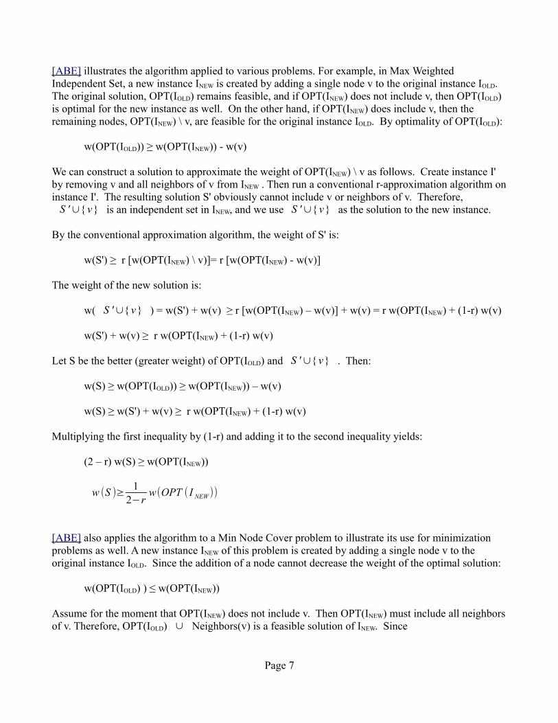
[ABE] illustrates the algorithm applied to various problems. For example, in Max Weighted Independent Set, a new instance INEW is created by adding a single node v to the original instance IOLD. The original solution, OPT(IOLD) remains feasible, and if OPT(INEW) does not include v, then OPT(IOLD) is optimal for the new instance as well. On the other hand, if OPT(INEW) does include v, then the remaining nodes, OPT(INEW) \ v, are feasible for the original instance IOLD. By optimality of OPT(IOLD):
w(OPT(IOLD)) ≥ w(OPT(INEW)) - w(v)
We can construct a solution to approximate the weight of OPT(INEW) \ v as follows. Create instance I' by removing v and all neighbors of v from INEW . Then run a conventional r-approximation algorithm oninstance I'. The resulting solution S' obviously cannot include v or neighbors of v. Therefore,
S ' ∪{ v} is an independent set in INEW, and we use S ' ∪{ v} as the solution to the new instance.
By the conventional approximation algorithm, the weight of S' is:
w(S') ≥ r [w(OPT(INEW) \ v)]= r [w(OPT(INEW) - w(v)]
The weight of the new solution is:
w( S ' ∪{ v} ) = w(S') + w(v) ≥ r [w(OPT(INEW) – w(v)] + w(v) = r w(OPT(INEW) + (1-r) w(v)
w(S') + w(v) ≥ r w(OPT(INEW) + (1-r) w(v)
Let S be the better (greater weight) of OPT(IOLD) and S ' ∪{ v} . Then:
w(S) ≥ w(OPT(IOLD)) ≥ w(OPT(INEW)) – w(v)
w(S) ≥ w(S') + w(v) ≥ r w(OPT(INEW) + (1-r) w(v)
Multiplying the first inequality by (1-r) and adding it to the second inequality yields:
(2 – r) w(S) ≥ w(OPT(INEW))
w (S )≥1
2−rw(OPT ( I NEW ))
[ABE] also applies the algorithm to a Min Node Cover problem to illustrate its use for minimization problems as well. A new instance INEW of this problem is created by adding a single node v to the original instance IOLD. Since the addition of a node cannot decrease the weight of the optimal solution:
w(OPT(IOLD) ) ≤ w(OPT(INEW))
Assume for the moment that OPT(INEW) does not include v. Then OPT(INEW) must include all neighborsof v. Therefore, OPT(IOLD) ∪ Neighbors(v) is a feasible solution of INEW. Since
Page 7

w(OPT(IOLD) ) ≤ w(OPT(INEW))
w(OPT(IOLD)) + w(Neighbors(v) ) ≤ w(OPT(INEW)) + w(Neighbors(v))
We can calculate a solution to approximate the weight of OPT(INEW) \ Neighbors(v) as follows. Create instance I' by removing v and all neighbors of v from INEW. Then run a conventional r-approximation algorithm on I'. The resulting solution S' obviously cannot include v or neighbors of v. Therefore, S' ∪ Neighbors(v) is a node cover in INEW, and is a solution to the new instance.
The weight of S', assuming v is not included in OPT(INEW), is:
w(S') ≤ r [w(OPT(INEW) - Neighbors(v)]
The weight of the new solution is:
w(S' ∪ Neighbors(v)) = w(S') + w(Neighbors(v))
≤ r [w(OPT(INEW) – w(Neighbors(v))] + w(Neighbors(v))
= r w(OPT(INEW) - (r-1) w(Neighbors(v))
Let S be the better (lower weight) of S' ∪ Neighbors(v) and OPT(IOLD) ∪ Neighbors(v). Then:
w(S) ≤ w(OPT(IOLD)) + w(Neighbors(v) ) ≤ w(OPT(INEW)) + w(Neighbors(v))
w(S) ≤ w(S' ∪ Neighbors(v)) ≤ r w(OPT(INEW) - (r-1) w(Neighbors(v))
Multiplying the first inequality by (r-1) and adding it to the second inequality yields:
r w(S) ≤ (2r - 1) w(OPT(INEW))
w (S )≤2r−1
rw (OPT ( I NEW ))
Finally, note that OPT(IOLD) ∪ {v} is feasible, and is optimal if OPT(INEW) includes v. Therefore, if this would be a better solution than S, i.e. if
w (OPT ( I OLD)∪{ v})=w (OPT ( I OLD))+w (v )≤w (S )
then we use OPT(IOLD) ∪ {v} instead of S as the solution.
The above approximation algorithm is also applicable when a constant number of nodes are added. When k nodes are added, there are (2k
- 1) subsets of new nodes. For each subset, we determine whether the subset possesses the desired hereditary property. For each that does possess the hereditary property, we make a similar assumption that the optimal solution to the new instance does or does not include that subset. The algorithm proceeds in an almost identical manner.
Page 8

2.3.3. A PTAS for certain unweighted hereditary graph problems with node insertions
Authors such as [ABE] and [BWZ] have described a PTAS for re-optimization of unweighted hereditary problems, under addition of a constant number of nodes. The hereditary property makes unweighted problems particularly simple. If a single (unweighted) node is inserted, the optimal value ofthe new instance can increase by at most 1.
|OPT(IOLD)| + 1 ≥ |OPT(INEW)|
In summary, if the number of nodes in w(OPT(INEW)) is 'small' we can find it by iteratively searching allsubsets of cardinality no greater than a constant. If on the other hand the number of nodes in w(OPT(INEW)) is 'large', then w(OPT(IOLD)) is a good approximation because it can differ by at most one.
Algorithm
For any ε > 0, set k=⌈1ϵ ⌉
Test all subsets of nodes of cardinality ≤ k for the desired hereditary property.Set S1 to be the subset with the desired hereditary property that has the greatest cardinality.Set solution S to be the better (greater cardinality) of S1 and OPT(IOLD)
If ∣OPT ( I NEW)∣≤k=⌈1ϵ ⌉ , S1 = OPT(INEW)
If ∣OPT ( I NEW)∣>k=⌈1ϵ ⌉ , then
∣OPT (I OLD)∣∣OPT (I NEW )∣
≥∣OPT (I NEW )∣−1
∣OPT ( I NEW )∣=1−
1∣OPT ( I NEW )∣
≥1−ϵ
This algorithm is not applicable to all hereditary problems. It requires not only the hereditary property, but also the ability to determine in polynomial time whether, for a given constant k, the optimal solution has value ≤ k. This property has been called simple, such as in [PM]. Some hereditary problems are not simple. For example, Min Coloring is a hereditary problem: if a graph can be colored with no more than k colors, all subgraphs can be colored with no more than k colors. However, deciding whether a graph can be colored with no more than three colors is NP-hard, so Min Coloring is not simple.
2.3.4. Hereditary graph problems with node deletions
In the literature on the re-optimization of hereditary graph problems, most often the local change is the addition of a node or a constant number of nodes. A few deal with node deletion, which makes the re-optimization problem more difficult. A primary difficulty caused by the deletion of nodes is that the solution to the previous instance may be significantly affected, and may not even be feasible any longer. The deleted node may have been an important part of the prior solution, and may even have been the entire solution.
Page 9

It is shown in [BMP] that if the number of deleted nodes could be an optimal solution for a hereditary problem, then the re-optimization problem is inapproximable within any ratio n-ε in polynomial time. In other words, an insurmountable obstacle is presented when k nodes are deleted, and it is possible that the optimal solution consists of k or fewer nodes.
This result has intuitive appeal. In essence, when the deletion of nodes could eliminate the entire solution that is available, we should not expect that knowledge of that solution could help us in solving the new instance.
The thrust of this general inapproximability result is best seen in problems where the size of the maximal solution is evident. For example, in [BMP] it is shown that the approximability of Max k-Colorable Subgraph under node deletion depends on whether the number of nodes deleted is the less than k. For this problem, a complete subgraph having k nodes is a maximal solution. If k or more nodes are deleted, then the entire solution is susceptible to deletion, and so we cannot approximate within any ratio n-ε in polynomial time. On the other hand, if h < k nodes are deleted, then at least a part of the solution (i.e. at least k – h nodes) is guaranteed to survive the deletion, so we can approximate to within:
k−hk
The proof provided by [BMP] assumes that any nodes may be deleted from the graph, including the entirety of the previous optimal solution. It would be interesting to investigate the inapproximability when there are greater restrictions on which nodes are deleted. For example, one possible restriction is that at least one node of the solution is guaranteed to be untouched by the deletion, or that node deletions are guaranteed to leave at least a certain fraction of the weight of the optimal solution intact.
An analogous difficulty can be seen in adding edges to an instance of Max Independent Set. If the newedges connect nodes of a previous optimal solution, then it is no longer even feasible. This is discussedbelow in Section 2.4.8
Page 10

2.4. Overview of Re-optimization Results for Specific Problems
This section briefly describes approximability results for the re-optimization of particular problems. In general, approximability depends not only on the problem but also on the type of local change that maybe made to the original instance of the problem. In many cases the approximation ratio of the re-optimization problem is significantly better than the ratio achievable for the conventional problem. For some problems, re-optimization provides a constant approximation ratio though the corresponding conventional problem has none. For some problems, lower bounds on approximability have been proven under certain types of local modifications.
2.4.1. Min Coloring
Where the local change is node addition, the re-optimization version of the Min Coloring problem has alower inapproximability bound of 4/3 – ε for any ε > 0, the same as the conventional Min Coloring problem.
This lower bound for re-optimization is quite evident from the fact that it is NP-hard to determine whether a graph can be colored with no more than three colors. As described in [ABE], starting with the empty graph and its trivial solution, the new instance is formed by adding a node. We use the re-optimization algorithm A to output a coloring of the new (single node) instance. We repeat this by continuing to add nodes. If A has an approximation ratio 4/3 – ε, then at each step A would output a 3-coloring if and only if the graph was 3-colorable. Obviously this would allow us to determine whether the graph is 3-colorable.
2.4.2. Max k-Colorable Subgraph
Tight inapproximability bounds for different local modifications are proven in [BMP]. If h nodes are added to the graph, the best ratio achievable is
max (k
k+h,12)
If h nodes are deleted, where h < k, the best ratio achievable is
k−hk
while if h ≥ k, there is no constant factor approximation. This bifurcation in results is caused by the ability of node deletion to eliminate the entire previous solution, as discussed above in Section 2.3.4.
Page 11

2.4.3. Min Traveling Salesman Problem
In the general case, re-optimization TSP is just as hard as conventional TSP. Under the local modification of increasing or decreasing the weight of a single edge, there is no polynomial time approximation algorithm. Various proofs are provided in [BFHKKPW-06], [BFHKKPW-07], and [ABE]. The same approximability result occurs where the change is the addition or deletion of a singlenode.
One very simple proof is shown in [ABE] for the deletion of a node. Consider a complete graph G with n nodes. Some edges have weight one, and all other edges have weight n 2p(n) + 1 for some polynomial p(n). Let G' be the subgraph of G from including only the edges of weight one. We are given an optimal solution to G: a tour T which includes only edges of weight one, so the weight of the tour T is n. The local change to instance G is to delete one node v. We easily see a Hamiltonian path P in the modified instance, namely the path induced by deleting the node v from the tour T. If a re-optimization algorithm could use G and T to approximate the optimal solution to the modified instance with a 2p(n) approximation ratio, this would tell us whether G' had a Hamiltonian cycle. It is NP-hard to determine, given a Hamiltonian path, whether a Hamiltonian cycle exists.
The authors of [BHS-2] show that even if all (possibly exponentially many) optimal solutions to the original instance are available, it remains NP-hard to compute a 2n approximation (even ignoring the size of the available optimal solutions).
For graphs which satisfy the triangle inequality, the re-optimization problem remains NP-hard but goodapproximation algorithms exist. Where the local change is a modified edge weight, there is a 7/5 approximation ratio. See for example [BHMW], [BFHKKPW-06], [BFHKKPW-07]. Where the local change is an added node, there is a 4/3 approximation ratio by [AEMP], which uses a modification of Christofides' algorithm.
There are similar results for non-metric graphs which satisfy the generalized triangle inequality:
w (u , v )≤β(w(u , x)+w( x , v )) ∀u , v , x∈V
In [BFHKKPW-06] it is shown that this generalized problem is NP-hard for all β > ½, but for all 1 < β < 3.35, a re-optimization algorithm can achieve a better approximation ration than the corresponding conventional algorithm.
2.4.4. Min Steiner Tree
Under the local modification of adding or deleting one terminal node, re-optimization of the Steiner tree problems remains strongly NP-hard, even if the set of permitted edge costs is restricted to {1, 2}. See for example the proofs in [BHKMR] and [BHMW]. If the set of permitted edge costs is restricted to {1, 2, 3, …, r}, the problem has a PTAS, as shown in [BHKMR] and [BHMW]. For general weights,there is a 3/2 approximation algorithm for adding or deleting one terminal node, as shown in [EMP],[BHKMR], and [BHMW]. In particular, the proof given in [EMP] essentially merges the solution of the original instance with Steiner trees computed on a set of newly added nodes. A similar proof gives
Page 12

a (3/2)-approximation ratio if the status of a node is changed from terminal to non-terminal or vice versa, as shown in [BHMW]. Under the local modification of increasing or decreasing the weight of one edge, the re-optimization version of the Steiner tree problems remains strongly NP-hard [BHMW]. However, there are 4/3 and 1.3 approximation algorithms, respectively, as described in [BBHKMWZ].
2.4.5. Max Knapsack
Since the conventional knapsack problem admits a FPTAS, the re-optimization version does as well. Therefore, re-optimization of the Max Knapsack problem focuses on improving the run time for a given approximation ratio, or on improving the approximation ratio for a given run time.
The authors of [ABS] employ an algorithm similar to that shown in Section 2.3 for hereditary graph problems to the 0-1 knapsack problem. Using any r-approximation algorithm for knapsack, the re-optimization version achieves a 1/(2 – r) ratio, which is strictly better than r. They also show a class of instances for which their algorithm is faster than the corresponding conventional PTAS or FPTAS algorithms.
2.4.6. Max Weighted Independent Set
An inapproximability result for Max Weighted Independent Set is shown in [BMP]. Any re-optimization algorithm, where the local change is addition of one node, and where the re-optimization algorithm utilizes approximations rather than optimal solutions, cannot have an approximation ratio better than ½, the same as returned by the simple constant time algorithm described in Section 2.3.1 for hereditary problems.
Re-optimization under edge deletions is more difficult than under node additions. However, a crucial insight is provided in [BWZ]. Given a set of k edges in any subgraph, the nodes of that subgraph can bepartitioned into l independent sets, where l is the constant positive integer that satisfies:
( l2)≤k<(l+1
2 )The authors use this insight to develop a re-optimization algorithm. A solution to the new instance is the better the previous solution and the greatest weight independent set among the endpoints of the deleted edges. Starting from any r-approximate solution to the original instance, the algorithm provides a tight approximation ratio:
rlr (l−1)+1
Re-optimization under addition of k edges is especially difficult. As in node deletion, edge insertion hasthe potential to destroy the previous solution. If the new edges connect nodes of a previous optimal solution, then it is no longer even feasible. In [BWZ] a solution to the new instance is formed by
Page 13

subtracting from the old solution all endpoints of added edges, and then adding back the greatest weight independent set among the endpoints of the added edges which were included in the old solution. Starting from any r-approximate solution to the original instance, and with l as defined above, the algorithm provides a tight approximation ratio:
rl
Page 14

2.5. Some Future Directions for Re-optimization
The results described above suggest many possible questions and areas for future re-optimization research. One of the most obvious is inapproximability bounds where none have yet been established, such as for the Min Steiner Tree problem.
The results summarized in Section 2.3 shows the benefit of techniques that can be applied to a broad class of problems. It would be interesting to formulate other broader classes of problems which are particularly amenable to facets of the re-optimization framework.
Most of the re-optimization literature involves the availability of one previous solution. We have seen in Section 2.4.3 that for the general TSP, the availability of all (possibly exponentially many) optimal solutions to the original instance do not help at all. There is potential in exploring whether and how much the knowledge of all, not merely one, previous optimal solution can help for different re-optimization problems.
As described above in Section 2.3.4, it is harder to solve certain graph re-optimization problems when the local change is the deletion, rather than the addition, of nodes. The difficulty is caused primarily by the fact that the deleted nodes may have been the entirety of the previous optimal solution. In other types of problems, different kinds of local changes would have a comparable effect on the previous solution. If these local changes were restricted so that they did not eliminate the entire previous solution, that might affect inapproximability of the problem.
Page 15

3. Some Original Results for Re-Optimization Problems
3.1. A Generalization of Hereditary Problems
Hereditary problems are outlined above in Section 2.3. The literature, such as [BMP] and [ABE], describes hereditary problems in terms of graphs and properties of certain graph nodes. Hereditary problems are particularly amendable to the re-optimization framework. Moreover, [ABE] explicitly recognizes that certain algorithms applicable to hereditary problems can also be applied to certain non-graph problems, such as Max Sat and Knapsack.
Clearly, the hereditary property is a sufficient condition that permits a graph problem to utilize the threeapproximation algorithms described above in Section 2.3. At the same time, the hereditary property is not necessary to utilize the techniques at more abstract level; these techniques have been applied to a few problems which do not fit the hereditary definition, and are not even graph problems.
The literature does not explain exactly which class of problems can use the three approximation algorithms presented for hereditary problems. Specifically, the literature does not describe which features a problem must possess in order to take advantage of these three approximation algorithms.
I have analyzed and extended the existing techniques for re-optimization of hereditary problems. Specifically, this section describes the following original results:
• a generalization of the three algorithms to a class broader than hereditary graph problems• a formal definition of the features that a problem must possess in order to use these algorithms• a PTAS for certain subclasses of weighted problems• an expansion of the types of local modifications from node addition to arbitrary modifications
Page 16

3.2. A Generalized Class of Problems for Added Components
The algorithms to be described in this section apply to the class of problems having the characteristics listed below. This class of problems encompasses hereditary graph problems as well as other problems which do not involve graphs at all. Re-optimization problems which fit this framework are amenable to
• a constant time (½)-approximation• a PTAS, provided the range of certain weights is bounded by a constant• an approximation ratio which is better than the approximation ratio of the conventional problem
Before describing the characteristics of problems in this class, the following term will be useful for purposes of exposition. The term does not entail any new concepts; it merely describes the conventional notion of objective functions.
DefinitionEvery instance of an optimization problem defines a set of components of the objective function, and each such component c has a positive weight w(c).
For example:In Max Weighted SAT, the objective function is the sum of the weights of clauses that are satisfied by a feasible solution. Since an instance of a problem is a CNF formula, the components of the instance are the clauses of the formula.
In Max Weighted Independent Set, the instance is a graph and the objective function is the sum of the weights of nodes included in a feasible solution. Therefore the components of the instance are the nodes of the graph.
In Knapsack, the objective function is the sum of the values of the items that are included in a feasible solution. An instance includes a set of items and the knapsack capacity. Therefore the components of the instance are the items.
In a Linear Program over decision variables xi with objective function max∑i=1
n
ci x i , the
components are the decision variables xi.
For an instance I, let ComponentsI denote the set of components for the instance. For any instance I, a feasible solution S defines the subset of ComponentsI which the solution satisfies:
components(S )⊆Components I
For a solution S of instance I, the weight of S, w(S), is simply the sum of the weights of the components in components(S)
w (S)= ∑ci∈components(S )
w (ci)
Page 17
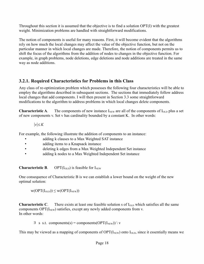
Throughout this section it is assumed that the objective is to find a solution OPT(I) with the greatest weight. Minimization problems are handled with straightforward modifications.
The notion of components is useful for many reasons. First, it will become evident that the algorithms rely on how much the local changes may affect the value of the objective function, but not on the particular manner in which local changes are made. Therefore, the notion of components permits us to shift the focus of the algorithms from the addition of nodes to changes in the objective function. For example, in graph problems, node deletions, edge deletions and node additions are treated in the same way as node additions.
3.2.1. Required Characteristics for Problems in this Class
Any class of re-optimization problem which possesses the following four characteristics will be able to employ the algorithms described in subsequent sections. The sections that immediately follow address local changes that add components. I will then present in Section 3.3 some straightforward modifications to the algorithm to address problems in which local changes delete components.
Characteristic A. The components of new instance INEW are all of the components of IOLD plus a set of new components v. Set v has cardinality bounded by a constant K. In other words:
∣v∣≤K
For example, the following illustrate the addition of components to an instance:• adding k clauses to a Max Weighted SAT instance• adding items to a Knapsack instance• deleting k edges from a Max Weighted Independent Set instance• adding k nodes to a Max Weighted Independent Set instance
Characteristic B. OPT(IOLD) is feasible for INEW
One consequence of Characteristic B is we can establish a lower bound on the weight of the new optimal solution:
w(OPT(IOLD)) ≤ w(OPT(INEW))
Characteristic C. There exists at least one feasible solution s of IOLD which satisfies all the same components OPT(INEW) satisfies, except any newly added components from v. In other words:
∃ s s.t. components(s) = components(OPT(INEW)) \ v
This may be viewed as a mapping of components of OPT(INEW) onto IOLD, since it essentially means we
Page 18

can extract from OPT(INEW) a portion which is feasible for IOLD.
Note that a consequence of Characteristic C is there exists a solution s such that in IOLD:
w(s) ≥ w(OPT(INEW)) – w(v)
and by optimality of OPT(IOLD), we can establish an upper bound on the optimum solution of INEW:
w(OPT(IOLD)) ≥ w(s) ≥ w(OPT(INEW)) – w(v)
w(OPT(IOLD)) + w(v) ≥ w(OPT(INEW))
Characteristic D. We can construct in polynomial time a solution s that is feasible for INEW and that satisfies the most weight possible in the set of new components v. In other words, the satisfied components of s, restricted to v, have the greatest weight of any solution t restricted to v.
∀t ∈Solutions( I NEW ) , w(uMAX )=w(components (s )∩v )≥w(components ( t)∩v )
Thus s may be viewed as the solution having the greatest weight that is mapped onto the new components v.
Note that hereditary graph problems, as typically defined for maximization problems, meet each of the four characteristics. This is explained in detail in Appendix A. Moreover, a larger class of problems alsomeets these characteristics, as shown in the examples in the sections that follow.
An important feature of problems in this class, for purposes of re-optimization, is that we can bound theweight of the new optimal solution. Specifically, the weight of the new solution is between the weight of the old solution and the old solution plus an additive amount.
For simplicity, in the remainder of this paper this class of problem is referred to as WEIGHT-ADD.
Page 19

3.2.2. A constant time (½)-approximation for WEIGHT-ADD problems
As described in Section 2.3.1, many authors have referred to the constant time (½)-approximation for hereditary graph problems in which a constant number of nodes is added to the graph. This algorithm isnow modified to apply to problems in WEIGHT-ADD.
AlgorithmBy Characteristic D, we can construct a solution s feasible for INEW and that satisfies the subset uMAX of v which has maximum weight of any feasible solution. By Characteristic B, OPT(IOLD) remains feasible for INEW. Let solution S be the better (greater weight) between OPT(IOLD) and s.
AnalysisSince s satisfies u, and possibly other components as well:
w(s) ≥ w(uMAX)
By definition of S:
w(S)=max[w(uMAX), w(OPT(IOLD))]
which of course means
w(S) ≥ w(uMAX)
w(S) ≥ w(OPT(IOLD))
adding these two inequalities:
2 w(S) ≥ w(OPT(IOLD)) + w(uMAX)
Next, by Characteristic C, there exists at least one feasible solution s' of IOLD such that
components(s') = components(OPT(INEW)) \ v
Also by Characteristic C, for any solution the heaviest contribution from components of v is w(uMAX):
w(s') ≥ w(OPT(INEW)) – w(uMAX)
and by optimality of OPT(IOLD):
w(OPT(IOLD)) ≥ w(OPT(INEW)) – w(uMAX)
Page 20

w(OPT(IOLD)) + w(uMAX) ≥ w(OPT(INEW))
combining this with the previous inequality gives:
2 w(S) ≥ w(OPT(INEW))
w(S )
w(OPT ( I NEW ))≥1/2
Page 21

3.2.3. A PTAS for certain WEIGHT-ADD instances
The algorithm below is based on the PTAS described in Section 2.3.3 for re-optimization of unweighted hereditary problems. This algorithm is polynomial if the range of (non-zero) weights is bounded by a constant.
In addition to the first four characteristics, the algorithm in this section requires a fifth characteristic:
Characteristic E. For any instance I and any subset u of ComponentsI having cardinality not greaterthan a constant, in polynomial time we can determine either:
a solution of I that satisfies all components of u (and possibly other components), orthat no feasible solution of I satisfies all components of u
For example, for Max Weighted Independent Set, we can determine in polynomial time whether any subset u of nodes is independent. However, many problems, including many hereditary problems, cannot satisfy this characteristic. For example, in a Min Coloring problem, components are 'colors'. Buteven for the constant number of three components, we cannot determine in polynomial time whether there is a feasible solution to satisfy all three components.
Appendix B shows how Characteristic E may be met in a Max Weighted k-SAT problem.
Assume without loss of generality that 0 < ε < 1.
AlgorithmConstruct a solution s that is feasible for INEW and that satisfies uMAX, the greatest portion of weight in v that any solution can satisfy.
If w (uMAX )
w(OPT ( I OLD))≤ϵ , then (CASE 1)
use OPT(IOLD) as the solution to the new instance INEW
Else if w (uMAX )
w(OPT ( I OLD))>
1ϵ , then (CASE 2)
use s as the solution to new instance INEW
Else (CASE 3)set WMIN = min weight of all components
set k=⌈w(uMAX )
ϵW MIN
⌉
for each subset of components of cardinality ≤ k, find a solution that satisfies those components
set S1 to be the solution with the largest total weight of these solutionsuse the better of OPT(IOLD) and S1 as the solution to the new instance INEW
Page 22

AnalysisFor the first step of the algorithm, Characteristic D allows us to construct s which satisfies the components of some subset uMAX of v in polynomial time. We can easily determine what uMAX is by determining all components of v that are satisfied by s.
Case 1:w (uMAX )
w(OPT ( I OLD))≤ϵ
By Characteristic C, there exists at least one feasible solution s' of IOLD which satisfies all the same components OPT(INEW) satisfies, except any newly added components from v. Let u' denote the components from v that OPT(INEW) satisfies:
u ' =components (OPT ( I NEW ))∩v
so the solution s' must have weight:
w(s') = w(OPT(INEW)) – w(u')
and by the optimality of OPT(IOLD):
w(OPT(IOLD)) ≥ w(s') = w(OPT(INEW)) – w(u')
Since the first step gives uMAX, the set of components of solution s such that
uMAX =components (s)∩v
and since by Characteristic D for any solution t of INEW
w (uMAX )=w(components (s)∩v)≥w(components (t)∩v)
we conclude:
w(uMAX) ≥ w(u')
which combined with the previous inequality yields:
w(OPT(IOLD)) ≥ w(OPT(INEW)) – w(u') ≥ w(OPT(INEW)) – w(uMAX)
We can use this inequality to determine the approximation ratio:
ratio=w(OPT (I OLD))
w(OPT (I NEW ))≥
w (OPT ( I NEW ))−w (uMAX )
w(OPT (I NEW ))=1−
w (uMAX )
w(OPT (I NEW ))
Page 23

By Characteristic B, OPT(IOLD) is also feasible for INEW. Therefore by the optimality of OPT(INEW):
OPT(IOLD) ≤ OPT(INEW)
ratio≥1−w (uMAX )
w (OPT ( I NEW ))≥1−
w (uMAX )
w(OPT (I OLD))≥1−ϵ
where the last inequality is by the assumption of case 1 that
w (uMAX )
w(OPT ( I OLD))≤ϵ
Page 24
Case 2:w (uMAX )
w(OPT ( I OLD))>
1ϵ
We use solution s as an approximation for OPT(INEW). Since s satisfies at least the components of uMAX:
ratio=w (s)
w(OPT (I NEW ))≥
w (uMAX )
w (OPT ( I NEW ))
As shown above in case 1:
w(uMAX )
w(OPT ( I NEW ))≥
w (OPT ( I NEW ))−w (OPT ( I OLD))
w(OPT (I NEW ))=1−
w(OPT (I OLD))
w(OPT (I NEW ))
Since s is feasible for INEW and s satisfies all components of uMAX, then by optimality of w(OPT(INEW)):
w(OPT(INEW)) ≥ w(s) ≥ w(uMAX)
Next, the condition of case 2 can be rewritten as:
w (uMAX )>(1ϵ )w(OPT ( I OLD))
Combining the previous two inequalities yields:
w (OPT ( I NEW ))>1ϵ w (OPT ( I OLD))
ϵ>w (OPT ( I OLD))
w(OPT (I NEW ))
Therefore:
ratio≥1−w(OPT (I OLD))
w (OPT ( I NEW ))≥1−ϵ
Case 3: w (uMAX )
w(OPT ( I OLD))>ϵ
Set WMIN to be the minimum weight of all components.
For k=⌈w(uMAX )
ϵW MIN
⌉ , test each subset of components that has cardinality not more than k for a feasible
solution (if any exists) which satisfies all components in the subset. By Characteristic E, in polynomial
Page 25

time we can find each such solution, or determine that no such solution exists.
If k is a constant, the number of subsets of cardinality ≤ k is polynomial by the simple upper bound:
∑i=1
k
(ni )≤k(n
k)=O(nk)
Since k depends on the ratio of certain weights of the problem, the run time is not polynomial. However, if the ratio of weights is bounded by a constant, then the run time is polynomial. The bounded weight range condition is, for some constant K:
w(uMAX )
W MIN
≤K
Therefore under a bounded weight range, k is also bounded by a constant:
k=⌈w(uMAX )
ϵW MIN
⌉≤⌈Kϵ ⌉
Since iterating over any set of cardinality ≤ k can be done in polynomial time, and since iterating over all subsets takes polynomial time, the entire process can be done in polynomial time.
Among all solutions found above, S1 is the solution with the greatest weight, and the solution S has weight:
w(S) = max(w(OPT(IOLD)); w(S1))
There are two possibilities, which we will call cases 3A and 3B, for the value of w(uMAX) in relation to the (unknown) weight of the new optimal solution. Although we cannot know whether we are in case 3A or 3B, in both the algorithm returns an acceptable approximation.
case 3A:w(uMAX )
w(OPT (I NEW ))≥ϵ
Since each component has weight at least WMIN, the least weight that a subset of (k+1) nodes could have is:
(k+1)W MIN=k W MIN +W MIN=⌈w(uMAX )
ϵW MIN
⌉W MIN+W MIN≥w(uMAX )
ϵ +W MIN
The condition for case 3A, which can be rewritten as an upper bound on the weight of the new optimal solution:
Page 26

w(uMAX )ϵ ≥w (OPT ( I NEW ))
Combining these two inequalities yields:
(k+1)W MIN≥w (uMAX )
ϵ +W MIN >w(uMAX )
ϵ ≥w(OPT ( I NEW ))
In other words, any solution which satisfies (k+1) or more components must have weight greater than the weight of the optimal value. Therefore, no such solution can exist, and OPT(INEW) must satisfy k or fewer components. Therefore the algorithm actually finds OPT(INEW):
S1 = OPT(INEW)
case 3B:w(uMAX )
w(OPT ( I NEW ))<ϵ
Combining the condition for case 3B with the condition for case 3 gives:
w (uMAX )
w(OPT ( I OLD))>ϵ>
w(uMAX )
w (OPT ( I NEW ))
which implies:
w(OPT(IOLD)) < w(OPT(INEW))
As described above for case 1, we can bound OPT(IOLD) from below with:
w(OPT(IOLD)) ≥ w(OPT(INEW)) – w(uMAX)
Therefore the approximation ratio can be bounded as follows:
ratio=max(w(OPT (I OLD)) ,w(S1))
w (OPT ( I NEW ))≥
w(OPT (I OLD ))
w (OPT ( I NEW ))
≥w (OPT ( I NEW ))−w (uMAX )
w(OPT ( I NEW ))=1−
w (uMAX )
w(OPT (I NEW ))≥1−ϵ
Page 27

3.2.4. An improved approximation ratio for WEIGHT-ADD problems
This algorithm is based on the PTAS described in Section 2.3.2 for re-optimization of hereditary graph problems.
In addition to the first four characteristics A - D, the algorithm in this section requires four additional characteristics, all four of which are possessed, for example, by hereditary graph problems:
Characteristic F. Any solution for INEW that doesn't satisfy any component of v is feasible for IOLD.
Characteristic G. If we knew that OPT(INEW) satisfied some subset u of v, we could construct in polynomial time an instance I'' whose optimal solution satisfied all the same components as OPT(INEW) except any components of u.
Note that this characteristic is similar to Characteristic C, which merely assumes the existence of a solution s such that that would satisfy such an instance I''.
Characteristic H. (relies on G for I'') We can in polynomial time generate an r-approximate solutionSapprox for instance I'' defined in Characteristic G, where 0 < r < 1. In other words,
w(Sapprox) ≥ r w(OPT(I''))
Note that, if Characteristic F is also valid, then the r-approximate solution to such an instance I'' would be feasible for IOLD.
Characteristic I. Given an Sapprox as in Characteristic H, and given any subset u of v which is satisfied by some solution of INEW, we can construct, in polynomial time, a solution S' to INEW such that S' satisfies everything Sapprox satisfies, as well as u:
components (S ' )=components (Sapprox)∪u , ∀u⊆v where ucan be satisfied by some solution
AlgorithmFor each subset ui of components of v for which a feasible solution satisfies all ui,
construct I''i as in Characteristic Ggenerate approximation Sapprox, i for I''i as in Characteristic Hconstruct S'i as in Characteristic I
Let S2 be the S'i with maximum weightLet solution S be the better (greater weight) of S2 and OPT(IOLD).
Page 28

ANALYSISSince by Characteristic A v has a constant number of elements, the number of subsets of v is also constant. We can construct each I''i in polynomial time by Characteristic G, so we can construct all such I''i in polynomial time. We can similarly construct each Sapprox, i and S'i by Characteristics H and I. Since there is a constant number of subsets, we can search all S'i in polynomial time to find S2, the S'i with maximum weight.
By Characteristic I, for each i the weight S'i is:
w(S'i) = w(Sapprox, i) + w(ui)
By Characteristic H we have a bound on the weight of the approximation:
w(Sapprox, i) ≥ r w(OPT(I''i))
so we conclude that for all i:
w(S'i) ≥ r w(OPT(I''i)) + w(ui)
By Characteristic G, we can express w(OPT(I''i)) in terms of w(OPT(INEW)):
w(S'i) ≥ r [w(OPT(INEW)) - w(ui) ] + w(ui)
By definition of S:
w(S)=max[w(S2), w(OPT(IOLD))]
which of course means
w(S) ≥ w(S2)
w(S) ≥ w(OPT(IOLD))
Since S2 is by definition the maximum weight S'i, for all i:
w(S2) ≥ w( Sapprox, i ∪ ui) = w(Sapprox, i) + w(ui)
w(S) ≥ w(S2) ≥ w(Sapprox, i) + w(ui) for all i
Let j be the (unknown) index such that uj is the portion of v satisfied by OPT(INEW):
OPT ( I NEW)∩v=u j
In other words, j is the index such that uj matches the subset of v included in OPT(INEW).Since the above inequality is true for all i, it is true for j:
w(S) ≥ w(Sapprox, j) + w(uj)
Page 29

We can combine this with the above inequality for the approximation:
w(S) ≥ w(Sapprox, j) + w(uj) ≥ r [w(OPT(INEW )) - w(uj)] + w(uj)
(*) = r w(OPT(INEW)) +(1-r) w(uj)
Next since:
w(S) ≥ w(OPT(IOLD))
we can bound this from below using Characteristic C and by optimality of OPT(IOLD):
w(S) ≥ w(OPT(IOLD)) ≥ w(s) = w(OPT(INEW)) – w(uj)
Next, multiply this inequality by (1-r), which doesn't change the direction of inequality since r < 1
(*) (1-r)w(S) ≥ (1-r)w(OPT(INEW)) – (1-r)w(uj)
Adding the two inequalities marked with (*) yields:
(2 – r) w(S) ≥ w(OPT(INEW))
w (S )≥1
2−rw(OPT (I NEW ))
Page 30

3.3. A Generalized Class of Problems for Deleted Components
The local modification to the problem instance may be the deletion, rather than addition, of components. For example, in a Max Independent Set problem, nodes may be deleted or edges may be added. Both changes can force a node in the previous solution to be removed for the new solution. For example, a node of the previous solution may have been the one deleted, or an edge may have been added between two nodes of the previous solution.
Handling the deletion of components requires that we slightly modify the characteristics defined in Section 3.2. As will be described below, in contrast to adding components, an additional challenge maybe how exactly to determine from the local change which components have been deleted.
Characteristic A'. The components of new instance INEW are all of the components of IOLD from which a set of components v have been removed. Set v has cardinality bounded by a constant K. In other words:
∣v∣≤K
For example, the following illustrate the deletion of components from an instance:• deleting k clauses from a Max Weighted SAT instance• deleting items from a Knapsack instance• adding k edges to a Max Weighted Independent Set instance• deleting k nodes from a Max Weighted Independent Set instance
Characteristic B'. OPT(INEW) is feasible for IOLD
One consequence of Characteristic B' is we can establish an upper bound on the weight of the new optimal solution:
w(OPT(IOLD)) ≥ w(OPT(INEW))
Characteristic C'. There exists at least one feasible solution s of INEW which satisfies all the same components OPT(IOLD) satisfies, except any newly deleted components from v. In other words:
∃s s.t.components (s)=components(OPT (I OLD)) \ v
This may be viewed as a mapping of components of OPT(IOLD) onto INEW, since it essentially means we can extract from OPT(IOLD) a portion which is feasible for INEW. Note that a consequence of Characteristic C' is there exists a solution s such that in INEW:
w(s) ≥ w(OPT(IOLD)) – w(v)
Page 31

and by optimality of OPT(INEW), we can establish a lower bound on the optimum solution of INEW:
w(OPT(INEW)) ≥ w(s) ≥ w(OPT(IOLD)) – w(v)
Characteristic D, which required a solution that satisfied the most weight possible in the added components, is not needed. However, as discussed below it may be analogously difficult to determine exactly which components have been deleted, and construct a solution that is feasible for the new instance.
Characteristic E. is unchanged
3.3.1. Max Weighted Independent Set with Added Edges
Next we illustrate the deletion of components using a Max Weighted Independent Set instance, to which edges are added. We use the PTAS in Section 3.2.3, assuming again that the range of weights is bounded by a constant.
The addition of edges to a Max Independent Set instance can change the feasibility of the previous optimal solution. If both endpoints of a newly added edge are included in the solution to the original instance, clearly both endpoints are no longer independent.
As discussed above in Section 2.4.6, [BWZ] show that for k added edges, the endpoints of those edges can be easily partitioned into l independent sets, where l is the constant positive integer that satisfies:
( l2)≤k<(l+1
2 )Let Ek be the (at most k) added edges that intersect nodes in OPT(IOLD), and let N be those nodes.We can partition the nodes of N into l independent sets {IS1, IS2, …, Isl}. We find the independent set has the most weight, and call it ISMAX.
If we remove the all nodes in N from OPT(IOLD):
OPT(IOLD) \ N
we have a set of independent nodes. To this we add ISMAX for our solution S:
OPT(IOLD) \ N ∪ ISMAX
Note then that the deleted components of this problem are:
N \ ISMAX
Page 32

In other words, the deleted components are not the deleted nodes. The nature of the problem was such that we were able to narrow the weight of what had to be deleted from a larger set of candidates, N, to asmaller set of actually deleted components: N \ ISMAX. Also, since ISMAX is the subset with maximum weight, and since there are l subsets, we can upper bound the weight of deleted components:
w(ISMAX) ≥ w(N) / l
w(N \ ISMAX) ≤ (1 – 1/l) w(N)
Armed now with the set of deleted components, which we continue to denote as v in the manner of Section 3.2, we can employ the PTAS described in Section 3.2.3 with minor modifications:
AlgorithmConstruct a solution s that is feasible for INEW, and for which components
uMAX ⊆vhave been deleted from OPT(IOLD), in other words
components(s) = components(OPT(IOLD)) \ uMAX
If w (uMAX )
w(OPT ( I OLD))≤ϵ , then (CASE 1)
use s as the solution to new instance INEW
Else (CASE 2)set WMIN = min weight of all components
set k=⌈w(uMAX )
ϵW MIN
⌉
for each subset of components of cardinality ≤ k, find a solution that satisfies those components
set S1 to be the solution with the largest total weight of these solutionsuse the better of s and S1 as the solution to the new instance INEW
AnalysisFor the first step of the algorithm, Characteristic D allows us to construct s which satisfies the components of some subset uMAX of v in polynomial time.
Case 1:w (uMAX )
w(OPT ( I OLD))≤ϵ
For the Maximum Independent Set example, we would use what we determined above:
s = OPT(IOLD) \ N ∪ ISMAX
whereuMAX = N \ ISMAX
Page 33

Thus:
s = OPT(IOLD) \ uMAX
Therefore the weights are:
w(s) = w(OPT(IOLD)) – w(uMAX)
ratio=w (s)
w(OPT (I NEW ))=
w (OPT ( I OLD))−w (uMAX )
w (OPT ( I NEW))≥
(1−ϵ)w(OPT (I OLD))
w(OPT (I NEW ))
Where the last is by the condition of Case 1.
By condition B':
w(OPT(IOLD)) ≥ w(OPT(INEW))
Therefore:
ratio≥1−ϵ
Page 34

Case 2: w (uMAX )
w(OPT ( I OLD))>ϵ
Set WMIN to be the minimum weight of all components, and as before assume the range of weights is bounded
w(uMAX )
W MIN
≤K
Therefore under a bounded weight range, k is also bounded by a constant:
k=⌈w(uMAX )
ϵW MIN
⌉≤⌈Kϵ ⌉
Among all solutions found, S1 is the solution with the greatest weight, and the solution S has weight:
w(S) = max(w(OPT(IOLD)); w(S1))
There are two possibilities, which we will call cases 2A and 2B, for the value of w(uMAX) in relation to the (unknown) weight of the new optimal solution. Although we cannot know whether we are in case 2A or 2B, in both the algorithm returns an acceptable approximation.
case 2A:w(uMAX )
w(OPT (I NEW ))≥ϵ
Since each component has weight at least WMIN, the least weight that a subset of (k+1) nodes could have is:
(k+1)W MIN=k W MIN +W MIN=⌈w(uMAX )
ϵW MIN
⌉W MIN+W MIN≥w(uMAX )
ϵ +W MIN
The condition for case 3A, which can be rewritten as an upper bound on the weight of the new optimal:
w(uMAX )ϵ ≥w (OPT ( I NEW ))
Combining these two inequalities yields:
(k+1)W MIN≥w (uMAX )
ϵ +W MIN >w(uMAX )
ϵ ≥w(OPT ( I NEW ))
In other words, any solution which satisfies (k+1) or more components must have weight greater than
Page 35

the weight of the optimal value. Therefore, no such solution can exist, and OPT(INEW) must satisfy k or fewer components. Therefore the algorithm actually finds OPT(INEW).
S1 = OPT(INEW)
case 2B:w(uMAX )
w(OPT ( I NEW ))<ϵ
As described above for case 1, the weight of s is:
w(s) = w(OPT(IOLD)) – w(uMAX)
Therefore the ratio is:
ratio=w (s)
w(OPT (I NEW ))=
w (OPT ( I OLD))−w (uMAX )
w (OPT ( I NEW))≥
w (OPT ( I NEW ))−w (uMAX )
w(OPT ( I NEW ))
Where the last inequality is due to condition B':
w(OPT(IOLD)) ≥ w(OPT(INEW))
Finally by the condition of Case 2B:
ratio≥1−ϵ
3.4. Probabilistic Distribution of Component Weights
The PTAS described above in Sections 3.2.3 and 3.3.1 requires that the range of certain component weights are bounded by a constant. We can relax this requirement, and require instead that the probability that any weights are 'too small' is 'very low'. If so, then it is very likely that the total contribution from such components is small enough to be safely ignored in the PTAS.
Therefore, we turn to a class of instances with certain probabilistic weight distributions. In particular, given w(uMAX) as described above, we select a threshold lowest weight WMIN so that the ratio w(uMAX)/WMIN is no more than a constant. We then set k as above:
k=⌈w(uMAX )
ϵW MIN
⌉
Assume the weights are independently distributed according to some random distribution. A sufficient
Page 36

condition is that, for any δ > 0, the probability that among all of the n components, with high probability the total number of 'small' weight components is less than a (sufficiently small) constant. Then the total contribution to the weight of the components the algorithm does not examine is less than this constant. If this constant is small enough, then the weight missed is negligible.
For concreteness and to avoid becoming overwhelmed with variables, we select very particular numbers, but it will be evident how to generalize to arbitrary constants. Assume that a weight is 'too small' if it is less than WMIN/100, and that we want to determine the probability that, among all n components, no more than 100 components are 'too small'. This allows a total contribution of no more than WMIN from all unexamined components.
Let p be the probability that any weight is less than WMIN/100X be the total number of components that have weight less than WMIN/100
We can employ multiplicative Chernoff bounds:
prob [X <(1−α)n p]≤e−α
2 n p2
Since we want no more than 100 'small' components:
(1 – α) n p ≤ 100
α≥1−100np
Therefore the probability can be rewritten as limited by some desired constant δ:
prob [X <100 ]≤e−(1−100
np)
2 n p2≤δ
We desire to find the maximum p that permits this desired goal. We can manipulate the right hand side to a simpler form as follows:
(1−100np
)2
p≥2n
ln1δ
p2−200
np+
1002
n2≥
2n
ln1δ
p
p2−(200
n+
2n
ln1δ) p+
1002
n2≥0
We can increase the left hand side in order to complete the square:
Page 37
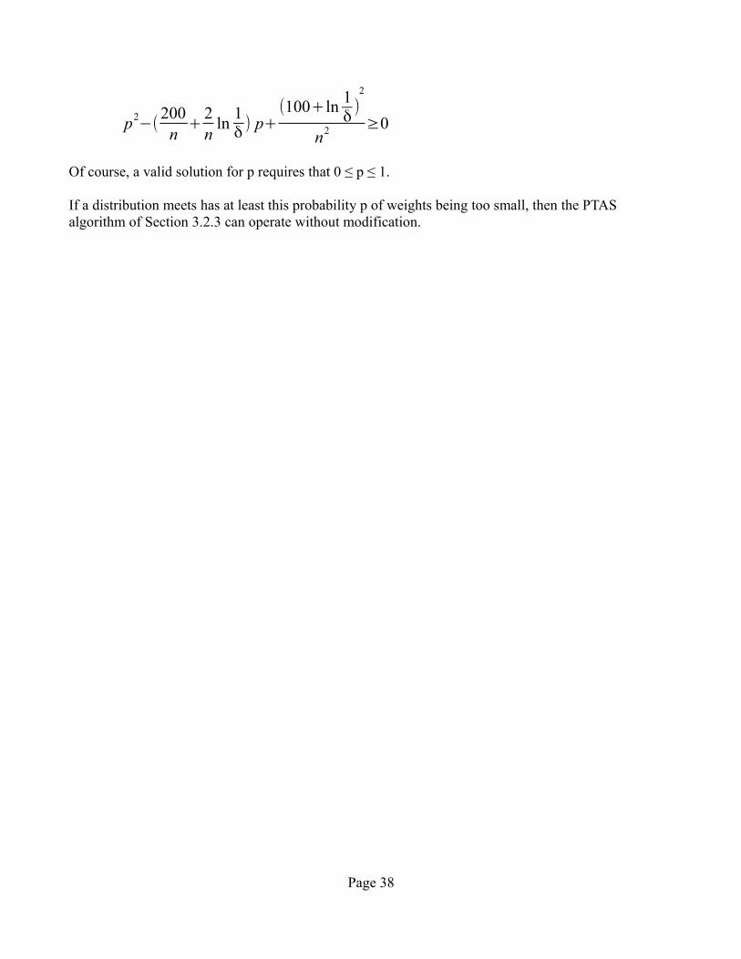
p2−(
200n
+2n
ln1δ) p+
(100+ln1δ)2
n2 ≥0
Of course, a valid solution for p requires that 0 ≤ p ≤ 1.
If a distribution meets has at least this probability p of weights being too small, then the PTAS algorithm of Section 3.2.3 can operate without modification.
Page 38

3.5. Future Work on the Generalized Class
It is hoped that others will improve and build upon this framework, investigate specific problems whichcan take advantage of the framework, and determine whether this framework can be generalized furtherto encompass a greater variety of problems. In addition, other algorithms besides the three presented may be developed for problems in this class.
In addition, I hope to expand the work in Section 3 to encompass a probabilistic distribution of weights and randomized approximation algorithms.
Page 39

4. Bibliography
[ABE] G.Ausiello, V. Bonifaci, B. Escoffier, Complexity And Approximation In Reoptimization, in “Computability in Context: Computation and Logic in the Real World”, B. Cooper, A. Sorbi Eds., Imperial College Press/World Scientific, pp. 101 - 130 (2009)
[ABS] C. Archetti, L. Bertazzi, M. Speranza, Reoptimizing the 0-1 Knapsack Problem, Discrete Applied Mathematics, Vol. 158, pp. 1879–1887 (2010)
[AEMP] G. Ausiello, B. Escoffier, J. Monnot, V. Paschos, Reoptimization of minimum and maximum traveling salesman's tours, in Proceedings of the 10th Scandinavian Workshop on Algorithm Theory, Lecture Notes in Computer Science, Vol. 4059, pp. 196-207 (2006)
[BBHKMWZ] D. Bilo, H. Bockenhauer, J. Hromkovic, R. Kralovic, T. Momke, P. Widmayer, A. Zych,Reoptimization of Steiner Trees, in Scandinavian Workshop on Algorithm Theory 2008, Lecture Notes in Computer Science vol. 5124, pp. 258-269 (2008)
[BFHKKPW-06] H. Bockenhauer, L. Forlizzi, J. Hromkovic, J. Kneis, J. Kupke, G. Proietti, P. Widmayer, Reusing Optimal TSP Solutions for Locally Modified Input Instances, Proceedings of the 4th IFIP International Conference on Theoretical Computer Science, pp. 251–270 (IFIP TCS 2006).
[BFHKKPW-07] H. Bockenhauer, L. Forlizzi, J. Hromkovic, J. Kneis, J. Kupke, G. Proietti, P. Widmayer, On the approximability of TSP on local modifications of optimally solved instances. Algorithmic Operations Research 2(2), pp. 83–93 (2007).
[BHKMR] H. Bockenhauer, J. Hromkovic, R. Kralovic, T. Momke, P. Rossmanith, Reoptimization of Steiner Trees: Changing the Terminal Set, Theoretical Computer Science, Vol. 410, Issue 36, pp. 3428–3435 (August 2009)
[BHMW] H. Böckenhauer, J. Hromkovič, T. Mömke, P. Widmayer, On The Hardness of Reoptimization, in Proc. of the 34th International Conference on Current Trends in Theory and Practiceof Computer Science (SOFSEM 2008),Lecture Notes in Computer Science, volume 4910, pp. 50 - 65
[BHS-1] H. Boeckenhauer, J. Hromkovic, A. Sprock, On The Hardness Of Reoptimization, Fundamenta Informaticae, Vol. 110, Issue 1-4, pp. 59-76 (2011).
[BHS-2] H. Boeckenhauer, J. Hromkovic, A. Sprock, Knowing All Optimal Solutions Does Not Help for TSP Reoptimization, Computation, Cooperation, and Life, Lecture Notes in Computer Science, Vol.6610, pp. 7-15 (2011)
[BMP] Boria, N.; Monnot, J.; Paschos, V.T., Reoptimization of some maximum weight induced hereditary subgraph problems, in LATIN 2012: Theoretical Informatics. Proceedings 10th Latin American Symposium, pp. 73-84 (April 2012)
Page 40

[BWZ] Davide Bilò, Peter Widmayer, Anna Zych, Reoptimization of Weighted Graph and Covering Problems, Approximation and Online Algorithms 6th International Workshop, WAOA 2008, vol. 5426, 2009, pp. 201-213 (September 2008)
[EG] S. Even and H. Gazit, Updating distances in dynamic graphs. Methods of Operations Research, 49:371–387 (1985).
[EMP] B. Escoffier, M. Milanic, V. Paschos, Simple and fast reoptimizations for the Steiner tree problem, Algorithmic Operations Research, Vol. 4, No. 2 (2009)
[F] G. Frederickson. Data structures for on-line updating of minimum spanning trees with applications. SIAM Journal on Computing, 14(4):781–798 (1985)
[PM] A. Paz and S. Moran, Non deterministic polynomial optimization problems and their approximations, Theoretical Computer Science, Vol. 15, pp. 251–277 (1981)
Page 41

Appendix A: Hereditary Graph Problems are a subclass of WEIGHT-ADD
Re-optimization of hereditary graph problems, where the local change is addition of a constant number of nodes and the objective is maximization, possesses all of the Characteristics required for membership in WEIGHT-ADD
Characteristic A.In a hereditary graph problem the components of the objective function are the weights of nodes havingthe desired hereditary property. Under the addition to the graph of v, a set of a constant number of nodes, the components are likewise increased by a constant number.
Characteristic B.When nodes are added to the graph, the previous solution remains feasible.
Characteristic C.Whatever nodes are included in OPT(INEW), we can take the difference
OPT(INEW) \ vand that (possibly empty) set of nodes is feasible in the original graph.
Characteristic D.Since v is a constant number of nodes, we can iterate through each possible subset of nodes, and for each determine if the subset satisfies the desired hereditary property. If so we can determine its weight,and take the solution that has the greatest weight of all such solutions.
Characteristic E.Similar to D above, for any constant number of nodes, we can iterate through each possible subset of nodes, and for each determine if the subset satisfies the desired hereditary property..
Characteristic F.Any solution for the graph that does not include the added nodes is feasible for the original graph.
Characteristic G.The ability to construct the required instance depends on the problem. For example, for Max Independent Set, we could construct such an instance by removing from the modified graph all new nodes and all neighbors of the new nodes.
Characteristic H.This depends on the availability of approximation algorithms for the problem.
Characteristic I.Since u is a set of nodes, we merely take the union of u and the approximate solution.
Page 42

Appendix B: Meeting Characteristic E for a Max Weighted k-SAT problem
Characteristic E requires that, for any instance I and any subset u of components, we determine in polynomial time either:
a solution of I that satisfies all components of u, orthat no feasible solution of I satisfies all components of u
Assume we have a Max Weighted SAT instance, and we are given a subset u consisting of a constant number C of clauses. Each clause includes no more than k literals. Therefore, the greatest number of variables involved in all C clauses is C k, a constant.
There are2C k
possible assignments to those variables, which is again a constant.
Therefore we can satisfy Characteristic E as follows.Iterate through all 2C k assignments of the C k variables of interestfor each such assignment, determine whether the assignment satisfies all C clausesif at least one such assignment satisfies all C clauses, return that assignmentif no assignments satisfy all C clauses, we know there is no variable assignment that can satisfy
those clauses (since the values of the remaining variables have no effect on these clauses).
Page 43