1. introduction molecular modeling & drug...

Chapter 1 Introduction

1

1. INTRODUCTION

1.1 Molecular Modeling & Drug Discovery

The average cost of developing new drug molecules and the time taken to

market them is pretty high. Although the time factor is getting reduced but the cost

factor is increasing further. Reasons for the growing expenses of pharmaceutical

companies include the investments needed for the new high throughput research

technologies [1] and for increase in the number of studies required for new drug

molecules [2]. However, even with the growing cost, the number of new drugs

coming to market has shown only a marginal increase. One of the reasons for this

trend could be lack of structural information about the target molecules. In the drug

design process enzymes are frequently the target of choice because of their

involvement in various biochemical pathways in human physiology. Even with

enzymes, there can be problems in obtaining their structural information. Sometimes

it is difficult to isolate or produce sufficient quantities of the target enzyme to study it

directly. These obstacles hinder the successful entry of drug candidates into market.

Therefore, there is an imperative demand for efficient methods that could enhance the

drug discovery process.

Computational methods or molecular modeling techniques can be utilized to

accelerate drug discovery process for obtaining new drug molecules. Today, almost

every multi-national drug company and Contract Research Organization (CRO)

involved in drug discovery has adopted computational methodology in different

stages of the design process. Many computational methods complement one another

and may be combined to help rationalize the drug discovery process. The ultimate

challenge in drug design is to predict and explain activities of new drug molecules [3].

Modern drug discovery is a multidisciplinary project, where the role of various

computational methods is to utilize experimental and predicted information in

designing new active compounds thereby facilitating and enhancing the rate of

discovery of appropriate chemical entities for lead optimization. As for as success

stories of drug molecules generated through molecular modeling is concerned, it has

been claimed that structure-based drug design methods have already contributed to

the introduction of some drug compounds into clinical trials and for drug approval [4,

5].


2

Currently two major molecular modeling strategies are employed in drug

design process, ligand-based drug design and structure-based drug design.

1.1.1 Ligand-based drug design

1.1.1.1 History of QSAR

To rationalize the drug design process, medicinal chemists frequently rely on

structure–activity relationships (SAR). An SAR is study of structural changes made to

a common core structure and observing how these changes affect activity. The

resulting SAR model is then useful in lead optimization, where functional groups

present on the core structure with physicochemical properties for high potency may be

further explored.

A natural extension of the traditional SAR is the quantitative structure–activity

relationship (QSAR), where some measures of chemical properties are correlated with

biological activity to derive a mathematical representation of the underlying SAR.

The first QSAR model was reported by Richardson in 1869 where the narcotic effect

of a series of alcohols was correlated with molecular weight [6]. QSAR was

revolutionized by Free-Wilson [7] and Hansch analysis [8] methods independently. A

more detailed review describing the development of QSAR has been reported by

Kubinyi [9, 10]. Although, the traditional QSAR models are useful for correlating

chemical properties of structure with the biological activity, they do not account for

how changes in three-dimensional molecular shape affect biological response. To

include shape-related descriptors in QSAR modeling, attention was given to the

development of 3D-QSAR. The first applicable 3D-QSAR method was introduced by

Cramer et al. [11] which compares the steric and electrostatic molecular fields

between a series of aligned molecules using PLS statistical analysis. The key

advantage in using molecular fields is that their contributions to the model can be

directly visualized in 3D, highlighting the structural features where changes can be

made to improve potency. The power of the approach is indicated by hundreds of

references that can be found in the literature applying the approach successfully to

drug design, as well as many extensions of the original methods (e.g. CoMSIA [12],

HINT [13], GRID/GOLPE [14], HASL [15], COMPASS [16] and AFMoC [17].


3

1.1.1.2 CoMFA Methodology

Comparative molecular field analysis (CoMFA) is the first approach with

electrostatic and steric interactions of molecules with their environment, taking into

account the 3D shape of the molecules. During the early stages of development of 3D-

QSAR, researchers recognized that protein–ligand interactions were mainly non-

covalent in nature. Based on this, it was thought that the electrostatic and steric

components from molecular mechanics force fields may provide sufficient

information to allow derivation of a predictive 3D-QSAR model. This was evaluated

and confirmed in 1988 with the successful development of predictive CoMFA model

for a set of steroids [11].

In CoMFA methodology the molecules of the data set need to be aligned

geometrically. Different alignment rules can be applied on the molecules of the data

set under study. The aligned molecules are then placed into cubic lattice one-by-one

and interaction energies between the molecule under study and a defined probe atom

(usually a proton or sp3 hybridized carbon atom with a positive charge) are calculated

for each lattice point. Each lattice point defines a position in space relative to the

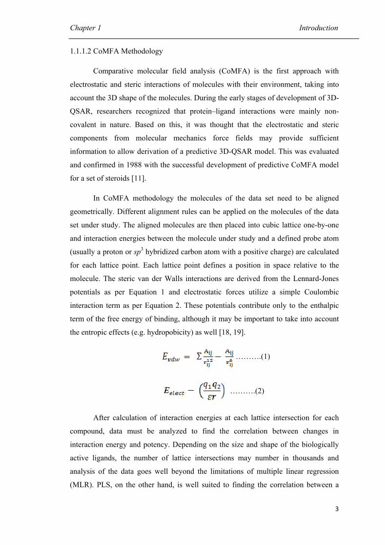
molecule. The steric van der Walls interactions are derived from the Lennard-Jones

potentials as per Equation 1 and electrostatic forces utilize a simple Coulombic

interaction term as per Equation 2. These potentials contribute only to the enthalpic

term of the free energy of binding, although it may be important to take into account

the entropic effects (e.g. hydropobicity) as well [18, 19].

……….(1)

……….(2)

After calculation of interaction energies at each lattice intersection for each

compound, data must be analyzed to find the correlation between changes in

interaction energy and potency. Depending on the size and shape of the biologically

active ligands, the number of lattice intersections may number in thousands and

analysis of the data goes well beyond the limitations of multiple linear regression

(MLR). PLS, on the other hand, is well suited to finding the correlation between a


4

small number of dependent variables and a large number of independent variables and

make the derivation of CoMFA models possible. In the iterative procedure of PLS,

new components (latent variables) are extracted so that each time, the degree of

commonality between the dependent and independent variables is minimized.

Usually, a maximum of five or six components are enough to generate a realistic

model. The optimum number of components is traditionally determined by cross-

validation, a technique that assesses the ability of a QSAR model to predict the

biological data. In this technique one or more compounds are left out from the model

and their biological activities are predicted on the basis of the model derived with the

remaining compounds. This procedure is repeated until each compound has been

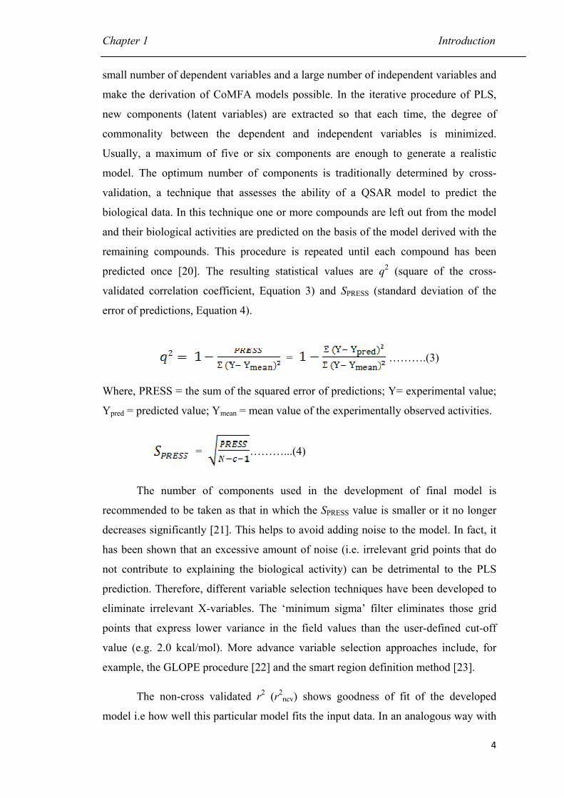
predicted once [20]. The resulting statistical values are q2 (square of the cross-

validated correlation coefficient, Equation 3) and SPRESS (standard deviation of the

error of predictions, Equation 4).

= ……….(3)

Where, PRESS = the sum of the squared error of predictions; Y= experimental value;

Ypred = predicted value; Ymean = mean value of the experimentally observed activities.

= ………...(4)

The number of components used in the development of final model is

recommended to be taken as that in which the SPRESS value is smaller or it no longer

decreases significantly [21]. This helps to avoid adding noise to the model. In fact, it

has been shown that an excessive amount of noise (i.e. irrelevant grid points that do

not contribute to explaining the biological activity) can be detrimental to the PLS

prediction. Therefore, different variable selection techniques have been developed to

eliminate irrelevant X-variables. The ‘minimum sigma’ filter eliminates those grid

points that express lower variance in the field values than the user-defined cut-off

value (e.g. 2.0 kcal/mol). More advance variable selection approaches include, for

example, the GLOPE procedure [22] and the smart region definition method [23].

The non-cross validated r2 (r2ncv) shows goodness of fit of the developed

model i.e how well this particular model fits the input data. In an analogous way with


5

q2 and SPRESS, r2 and the corresponding standard deviation can be calculated by

replacing Ypred with Ycal (activity value calculated by the model) in Equation 3 and 4.

The predictive r2 (r2pred) is obtained if the model is used to predict the activities of a

set of compounds not included in the model [20].

1.1.1.3 Modifications in CoMFA methodology

Perhaps the single most important drawback for CoMFA analyses is the

sensitivity of the technique to the alignment of the input structures, and usually a

structural scaffold is required to make this consistent, which also makes CoMFA most

applicable within congeneric series. To avoid the alignment problem, several

modifications have been made into the original method. Pastor et al. have developed

the Grid independent (GRIND) descriptors approach [24], whereby GRID MIFs for

each molecule are filtered by energy and MIF node pair distance. The GRIND

descriptors represent the product of the interaction energy for each pair of nodes,

binned by distance, with only the maximum products being retained. After statistical

analysis such as PLS, the QSAR model is obtained and the strongest contributions can

be traced back to the node pairs (analogous to pairs of pharmacophore points) which

can then give insight into improving activity. Recently, a modification that increases

the specificity of the descriptors has also been described [25], and it also improves the

MIF point sampling. It should be noted that in such an approach, finding appropriate

molecular conformation is still a challenging task. Additionally, another GRID-based

method has been developed that compresses the 3D GRID maps into a few

quantitative 2D descriptors; typically more relevant for ADME modelling, it has also

been used successfully to model the SAR of anti-HIV quinolones [26]. The topomer

descriptors discussed above have also been used in the CoMFA context, solving the

alignment and conformation problems. The topomers are generated by deterministic

rules that consistently describe fragments in 3D and are aligned according to

predetermined rules. However, this does require the compounds to share some kind of

common core or ‘equivalent’ acyclic bond where the structures are split into

fragments for comparison. Once the topomers have been generated (and with them the

alignments), the CoMFA statistical analysis is performed with a few minor

modifications to ‘standard CoMFA’ [27]. The approach by Vinter et al. for solving

the conformational problem is to compare the XED (Extended Electron Distributions)

-derived field minima points between pairs of active structures, in each case


6

considering several generated conformations. Cross-correlating these pairs, or duos,

from several active molecules yields the bioactive conformation hypothesis. Aligning

other active structures to this field template provides a combined field and volume

score that has been shown to correlate well with activity and exhibits reasonable

predictivity [28].

1.1.1.4 CoMSIA Methodology

The comparative molecular similarity indices analysis (CoMSIA) method was

developed to improve the limitation of the potentials used as steric and electrostatic

fields in CoMFA. Thus, CoMSIA method is useful to evaluate hydrophobic, hydrogen

bond donor and hydrogen bond acceptor characters along with steric and electrostatic

properties of molecules. In-fact, the original version of CoMSIA includes the

calculation of steric, electrostatic and hydrophobic fields; H-bond donor and acceptor

fields have been introduced later into the method [29]. In CoMSIA methodology,

instead of field descriptors based on Lennard-Jones- and Coulomb-type potentials,

molecular descriptors based on similarity indices of the aligned molecules are

computed. The energy potentials used in COMFA are very steep near the van der

Waals surface of the molecules and they produce singularities at the atomic centers. In

order to avoid too large energy values, arbitrary cut-off values have to be defined and

evaluation of the potentials are restricted to regions outside the molecules. To

overcome such problem, CoMSIA utilizes a Gaussian-type function for the distance

dependence between the probe and the atoms of the data set molecules (Equation 5).

. ............(5)

where ωik is the value of property k of atom i. The properties include a steric

contribution as a third power of atomic radii, electrostatic properties as pre-calculated

point charges, atom-based hydrophobicity parameters and representative positions of

H-bond donor and acceptor distribution. The properties ωprobe,k of the utilized probe

include a radius of 0.1 nm, +1 charge, +1 hydrophobicity, and +1 for both H-bond

donor and acceptor properties.


7

The similarity indices can be calculated at all grid points inside and outside the

molecule using a common probe which is placed at intersections of a regularly

sampled 3D grid box similar to CoMFA. A grid resolution of 0.1 nm, a grid box

extension of 4.0 nm and an attenuation factor α of 0.3 were used in the original

CoMSIA report [12]. This makes CoMSIA relatively intensive to changes in grid

spacing or orientation of the aligned molecules with respect to the lattice [30].

Statistical evaluation of similarity indices is done by PLS in the same way as in

CoMFA.

1.1.1.5 Advantages of CoMSIA over CoMFA

The Gaussian function used in CoMSIA methodology for calculating distance

dependence (ri - rj), requires no definition of a cut-off for field values. CoMSIA is not

so sensitive to changes in orientation of the superimposed molecules than CoMFA, or

to translations and rotations of the compound set with respect to the grid box [30].

Hence, CoMSIA may result in better predictive values. A third benefit for CoMSIA

over CoMFA is the better visualization and interpretation ability for the regions that

are predicted to be important for activity. In CoMFA these regions are highlighted as

contour maps in the 3D space that surrounds molecules [11], whereas in CoMSIA, the

regions are located within space that is occupied by the molecules and thus, directly

pinpointing structural features that are important for activity [31].

1.1.1.6 Validation of QSAR models

The process of QSAR model development is divided into three steps. The first

stage includes the selection of data set for QSAR studies and the calculation of

molecular descriptors. The second stage deals with the selection of a statistical data

analysis technique for correlation. The correlation process can not be done using

standard multiple linear regression (MLR) methods due to the huge number of

investigated independent variables [9]. Instead, a partial least square (PLS) analysis

[32] is the method of choice. PLS extracts principle component vectors (PCs), which

are obtained as linear combinations of the original independent variables in order to

maximize the correlation between independent and dependent variables. All PCs are

orthogonal; therefore, a new PC can be used in explaining only the data that is not

already described using the existing PCs. The final part of QSAR model development

is model validation in which estimates of the predictive power of the model are


8

calculated. The validation of a method is done to establish the reliability and

relevance of the method for a particular purpose. Reliability refers to the

reproducibility of results, the relevance is related to the scientific use and practical

usefulness and the purpose refers to the intended application. This predictive power is

one of the most important characteristics of QSAR models.

To evaluate the predictive ability, 3D-QSAR model need to be cross-validated

using optimum number of principle components [9, 20, 33]. Cross-validation can be

carried out by using leave-one-out procedure. In leave-one-out procedure, cross-

validation is carried out by omitting one compound at a time from the model building

and then predicting its activity with a model that is generated from the rest of the

compounds. The same procedure has been repeated for each individual compound.

The outcome of this procedure is a cross-validated correlation coefficient q2, which is

calculated according to the Equation 3

A random group cross-validation procedure should be repeated several times

as the difference in distribution of the compounds in the group during each PLS

analysis affects the q2 value. Clark et al. studied that a q2 value that is greater than

0.25 is very unlikely to result from a chance correlation [34] and q2 above 0.3

indicates that probability of chance correlation is less than 5% [35]. Many authors

consider high q2 (> 0.5) as an indicator or the proof of higher predictive power of the

developed QSAR model. They do not test the model for their ability to predict the

activity of the compounds outside the training set (test set) and they claimed that these

models were highly predictive. Thus, every QSAR model should be characterized by

a reasonably high q2 for their ability to accurately predict the biological activities of

compounds not included in the training set.

To establish model robustness, Y-Randomization of response is another

important validation criterion. The method consists of repeating the QSAR model

derivation calculation procedure, but with randomized activities. The subsequent

probability assessment of the resultant statistics is then used to gauge the robustness

of the model developed with the actual activities. It is often used along with the cross-

validation. If all QSAR models obtained in the Y-randomization test have relatively

high R2 and LOO q2, it implies that an acceptable QSAR model cannot be obtained for

the given data set by the current modeling methods.


9

It is still common not to test QSAR models (characterized by a reasonably

high LOO q2) for their ability to predict accurately biological activities of compounds

from an external test dataset, i.e. those compounds, which were not used for the model

development. The high q2 does not imply automatically a high predictive ability of the

model. In order to both develop the model and validate it, one needs to split the whole

available dataset into the training and test set. In fact, the lack of correlation between

the high value of the training set q2 and the high predictive ability of a QSAR model

has been noticed earlier in the case of 3D QSAR [36-38]. These studies indicated that

while high q2 is the necessary condition for a model to have a high predictive power,

it is not a sufficient condition. The only way to estimate the true predictive power of a

model is to test it on a sufficiently large collection of compounds from an external test

set.

Even today, many studies continue to consider q2 as the only parameter

characterizing the predictive power of QSAR models. Tropsha et al. have

demonstrated the insufficiency of the training set statistics for developing externally

predictive QSAR models and formulated the main principles of model validation [39],

and incorporated new rigorous validation criteria. According to Tropsha et al. a good

model should qualify in the following criteria:

a) q2 > 0.5

b) r2 > 0.6

c) [(R2 – R02) / R2] < 0.1 [(R2 – R´0

2) / R2] < 0.1

d) 0.85 ≤ k ≤ 1.15 or 0.85 ≤ k´ ≤ 1.15

where q2 is the cross-validated correlation coefficient; R2 or r2 is the correlation

coefficient for the experimental (y) vs. predicted (ỹ) activities for the test set

molecules; R02 and R´0

2 are the correlation coefficients for the regression line passing

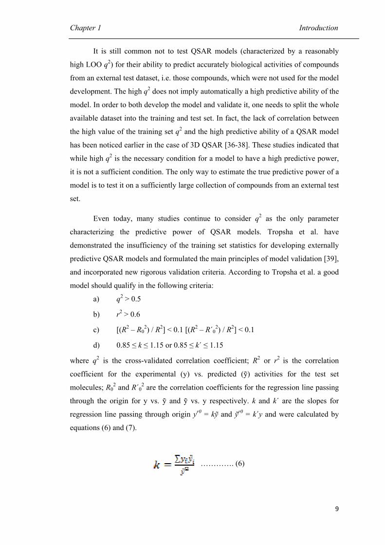
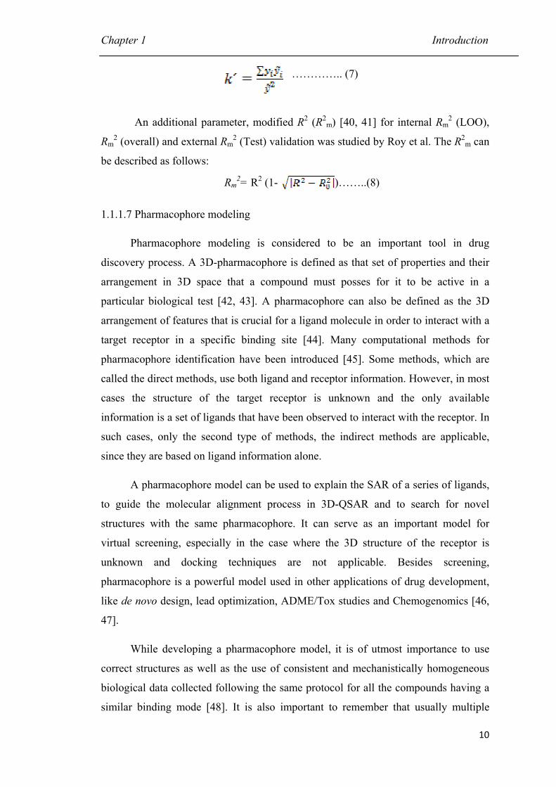
through the origin for y vs. ỹ and ỹ vs. y respectively. k and k´ are the slopes for

regression line passing through origin yr0 = kỹ and ỹr0 = k´y and were calculated by

equations (6) and (7).

…………. (6)


10

………….. (7)

An additional parameter, modified R2 (R2m) [40, 41] for internal Rm

2 (LOO),

Rm2 (overall) and external Rm

2 (Test) validation was studied by Roy et al. The R2m can

be described as follows:

Rm2= R2 (1- )……..(8)

1.1.1.7 Pharmacophore modeling

Pharmacophore modeling is considered to be an important tool in drug

discovery process. A 3D-pharmacophore is defined as that set of properties and their

arrangement in 3D space that a compound must posses for it to be active in a

particular biological test [42, 43]. A pharmacophore can also be defined as the 3D

arrangement of features that is crucial for a ligand molecule in order to interact with a

target receptor in a specific binding site [44]. Many computational methods for

pharmacophore identification have been introduced [45]. Some methods, which are

called the direct methods, use both ligand and receptor information. However, in most

cases the structure of the target receptor is unknown and the only available

information is a set of ligands that have been observed to interact with the receptor. In

such cases, only the second type of methods, the indirect methods are applicable,

since they are based on ligand information alone.

A pharmacophore model can be used to explain the SAR of a series of ligands,

to guide the molecular alignment process in 3D-QSAR and to search for novel

structures with the same pharmacophore. It can serve as an important model for

virtual screening, especially in the case where the 3D structure of the receptor is

unknown and docking techniques are not applicable. Besides screening,

pharmacophore is a powerful model used in other applications of drug development,

like de novo design, lead optimization, ADME/Tox studies and Chemogenomics [46,

47].

While developing a pharmacophore model, it is of utmost importance to use

correct structures as well as the use of consistent and mechanistically homogeneous

biological data collected following the same protocol for all the compounds having a

similar binding mode [48]. It is also important to remember that usually multiple


11

pharmacophore alignments are possible for a data set. The quality of a pharmacophore

model can only be measured by the models’ success in prospective application to drug

design i.e. how well it can facilitate lead optimization and the accuracy in selection of

active compounds to be synthesized, or how many active hits can be found in virtual

screening with a query based on the model [48].

Drug-like molecules may adopt many possible conformations. The specific

conformations that the input ligands adopt in the active site of the receptor are usually

unknown. Additionally, they cannot be assumed to be the ones with the lowest energy

[49]. Therefore, all the feasible conformations of the ligands should be considered

during the search for the common pharmacophore. Most methods perform the

conformational search in the initial stage. Examples for such methods include RAPID

[50] MPHIL [51] DISCO [52, 53] PHASE [54] Catalyst/HipHop [55-59]

Catalyst/HypoGen [55, 59, 60] and others [61-63]. These methods generate a discrete

set of conformations for each ligand with the goal of covering its whole

conformational space. Recently, Schneidman-Duhovny et al. [64] reported first web

server for detecting 3D pharmacophores shared by known active ligands in the

absence of structural information on the target receptor. It has been demonstrated that

the deterministic and efficient algorithm behind the server allows a fast and reliable

detection of pharmacophores with explicit consideration of the flexibility of the

ligands. Dror et al. [65] showed that pharmacophore hypothesis generated by

PharmaGist web server were found to be similar to a pharmacophore hypothesis

computed by Catalyst which confirms the efficiency and reliability of PharmaGist

web server.

1.1.2 Structure-based drug design

1.1.2.1 Molecular Docking

"Molecular docking" explores the binding modes of two interacting molecules,

depending upon their topographic features or energy-based considerations [66], and

aims to fit them into conformations that lead to favourable interactions. It therefore

constitutes an essential step in determining the active conformation of a drug, i.e. its

conformation when bound to the receptor. Hence, prediction of binding orientations

of small molecules in a protein/DNA binding site has become increasingly important

in drug design. Although it is possible experimentally to elucidate the structure of


12

protein–ligand complexes using crystallographic or nuclear magnetic resonance

(NMR) methods, it would be difficult to do so for all ligands in a medicinal chemistry

project. Molecular docking may provide this important information. Docking is often

approximated to a Lock and Key process where the conformation of a ligand and

receptor do not change during binding. This is the simplest to simulate, but is

generally thought to be unreasonable. Ligands are often flexible and occupy multiple

conformations in solution. Although, the conformations of receptors are better

defined, they too can change, particularly on ligand binding in the so called Induced

Fit model. Molecular Docking has a wide variety of uses and applications in Drug

Discovery, including structure activity studies, lead optimization, finding potential

lead by virtual screening, providing binding hypothesis to facilitate prediction of

mutagenesis studies, assisting X-ray crystallography in the fitting of substrate and

inhibitors to electron density, chemical mechanism studies and combinatorial library

design.

Large number of docking program are available for use in virtual screening

and every program has different algorithms to handle ligand and protein flexibility,

scoring functions and CPU time to dock a molecule to a given target. If in the process

of docking, both ligand and the target are treated as rigid bodies [67], the

conformational flexibility of ligands can be taken into account by creating a collection

of conformers and docking each one of them separately into target site. Instead, the

conformational search of ligands can be explored during the docking process. Some

examples of semi-flexible docking approaches also exist viz. incremental growth

methods [68], genetic algorithm (e.g. GOLD) [69], Tabu search (e.g. PRO_LEADS)

[70], and combined Monte Carlo and simulated annealing methods (e.g. Dock Vision)

[71]. Molecular docking using rigid protein is sometimes an inaccurate

approximation, since the binding of a ligand can induce large conformational changes

in a receptor binding site [72, 73]. One option to consider protein flexibility is to use

an ensemble of protein conformers. Example of such a docking program is FlexE,

wherein various protein conformers are superimposed and it treats the dissimilar

protein regions as distinct alternatives [74].

Once a pose has been generated for a ligand in the binding site, scoring

function needs to be applied to rank the quality of the pose with respect to other poses

of the compound based on binding energy of association of each pose. Scoring


13

function estimates the free energy of binding of a ligand in a target-ligand complex.

Scoring functions are used to optimize the placement of the ligands during the

docking process and are applied to rank the resulting ligand poses with respect to the

other poses and ligands [75, 76]. There are wide choices of scoring functions

available that are grouped into force-field based, empirical and knowledge-based

functions [77]. It is a well known fact that these fast scoring methods do not perform

so accurately as the time-consuming free energy perturbation technique [78]. Using a

combination of one or more scoring functions (i.e. consensus scoring) has been

reported to improve the results [79-81].

Some of the docking programs which are used in drug designing are

AUTODOCK [82], CDOCKER [83], DOCK [84], FlexX [85, 86], GOLD [87],

GLIDE [88, 89].

1.2 Telomerase and Cancer

1.2.1 Telomerase

Telomerase enzyme was first discovered in the unicellular ciliate,

Tetrahymena where it was shown to use an unusual mode of DNA synthesis for

polymerization of telomeric DNA [90, 91]. It is a catalytically active

ribonucleoprotein enzyme that consists of two major components, a reverse

transcriptase catalytic subunit (hTERT 127 kD; Gene ID 7015) and an RNA subunit

(hTR; Gene ID 7012). The RNA subunit functions as a template for synthesis of

telomeric DNA with the help of TERT directly on to the 3´ end of the chromosomes.

The amino-terminal moiety of the TERT protein is essential for the nucleolar

localization, and multimerisation. The COOH-terminal region is involved in the

processivity of the enzyme and is indispensable for in vivo activity [92]. The central

region contains the motifs characteristic of reverse transcriptase proteins and a

conserved RNA-binding domain required for specific binding of hTR by the hTERT

subunit [93]. The human telomerase RNA (hTR) extends on 451 nucleotides and

contains 11-nucleotide long template sequence for telomeric repeat synthesis. Ten

conserved helical regions were proposed in vertebrate telomerase RNA including four

distinct structural domains: the pseudoknot domain, the CR4eCR5 domain, the Box

H/ACA domain and the CR7 domain [94]. Earlier it was shown [95] that dyskerin


14

(57 kD) interacts with hTR; however, it has been proved very recently that the

presence of dyskerin protein is essential for the catalytic activity of the enzyme [96].

There is considerable evidence from in vitro reconstitution studies that telomerase

exists as a dimer [97, 98]; therefore, it was proposed that the catalytically active

human telomerase is composed of two molecules each of hTR, hTERT and dyskerin

(about 670 kD). The enzyme is almost undetectable in most normal somatic cells

except in proliferative cells of renewing tissue [99, 100]. However, recent evidence

shows that a small amount of the enzyme activity is detectable in normal cells also as

they enter S-phase but disappear when the cells go into G2-phase [101]. Telomerase

enzyme is involved in telomere capping [102] and in the DNA-damage response

[103].

In addition to TR and TERT, more than 30 proteins have been proposed to be

associated with the enzymatic telomerase complex [104].

1.2.2 Telomeres

Human telomere (telos = end; meros = part) consists of tandem repeats of the

hexameric DNA sequence TTAGGG, ranging from 15 kb at birth and less than 5 kb

in chronic diseases. Telomeres are dynamic nucleoprotein complexes that cap the

ends of linear eukaryotic chromosomes [105]. The role of telomeres for chromosome

stability was reported in the early 1940s by experiments in maize [106]. Telomeres

have two important duties. First, they protect the chromosome ends from destructive

nucleases and other damaging events e.g. end-joining. Second, they enable the ends to

be completely replicated. Due to the nature of lagging strand DNA synthesis,

conventional DNA polymerases are unable to completely replicate the ends of

chromosomes resulting in loss of 50-100 bp of telomeric DNA replication [107]

The fact that these bases do not code for any genetic information does not

diminish their importance. It is now know that they are a site of dynamic activity

beyond being the biologic timepiece [108]. They have a unique T-looped

configuration where the telomere bends back on itself [109]. The overhanging

guanine-rich single strand is placed into the double stranded telomere. This creates a

second smaller d-loop by displacing one of the telomere strands. This structure

appears to protect the telomeres from end to end fusion with other chromosomes and


15

from cell cycle checkpoints that would otherwise recognize the telomeres as

chromosome breaks requiring repair (reviewed in [110]).

1.2.3 Role of telomerase in cancer

1.2.3.1 Experimental evidences

During the past decade, more than 500 research/review articles have been

published on telomerase. The first detection of telomerase was done in ovarian cancer

in 1994 [111]. Nearly the complete spectrum of human tumors has been shown to be

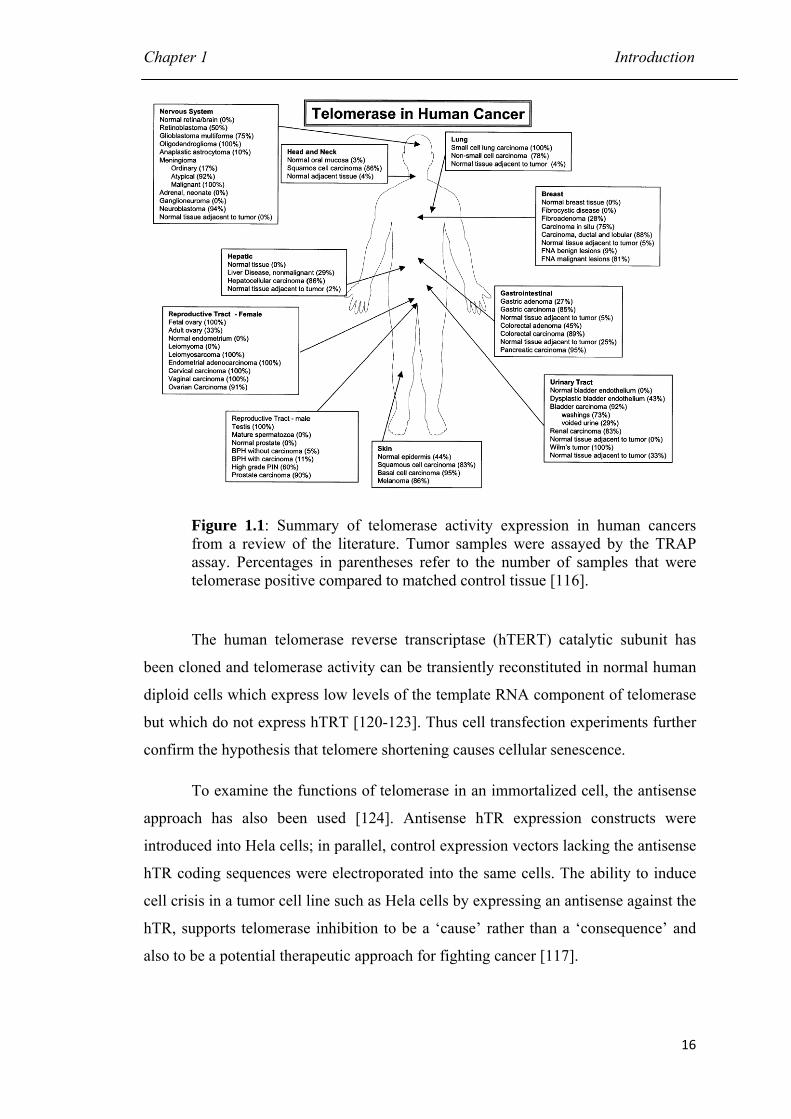
telomerase positive (Figure 1.1). One of the largest compilations of telomerase

activity in human tumor tissues has been recently published [112]. In this series which

include 601 human tumor samples, telomerase was detected in 476 samples (79%). So

much high percentage makes telomerase both an attractive cancer marker and a cancer

target [113]. Experimental result of a wide series of 100 neuroblastoma suggests that

the telomerase expression could be responsible in the evolution of neuroblastoma

[114]. Considering normal tissues, telomerase is present in normal human white blood

cells at very low level. Telomerase is also detected at low levels in germline tissues

and in some mitotic stem cells from normal epithelia [115].

Taken all together, clinical pharmacology data support the concept that

telomerase is a relevant target in oncology. The expression of telomerase between

normal and tumor tissues is indeed remarkable and largely superior to those observed

for classical chemotherapeutic targets such as topoisomerases, tubulin/microtubules,

enzymes implied in DNA metabolism/replication. This suggests that antitelomerase

treatment would turn in low toxicity for normal tissues [117].

To demonstrate whether telomerase is required for cell viability and tumor

formation, knockout mice were reared by elimination of the gene encoding the

telomerase RNA component [118] which gave an additional clue that the telomere-

associated events are indeed relevant to carcinogenesis [119].


16

Figure 1.1: Summary of telomerase activity expression in human cancers from a review of the literature. Tumor samples were assayed by the TRAP assay. Percentages in parentheses refer to the number of samples that were telomerase positive compared to matched control tissue [116].

The human telomerase reverse transcriptase (hTERT) catalytic subunit has

been cloned and telomerase activity can be transiently reconstituted in normal human

diploid cells which express low levels of the template RNA component of telomerase

but which do not express hTRT [120-123]. Thus cell transfection experiments further

confirm the hypothesis that telomere shortening causes cellular senescence.

To examine the functions of telomerase in an immortalized cell, the antisense

approach has also been used [124]. Antisense hTR expression constructs were

introduced into Hela cells; in parallel, control expression vectors lacking the antisense

hTR coding sequences were electroporated into the same cells. The ability to induce

cell crisis in a tumor cell line such as Hela cells by expressing an antisense against the

hTR, supports telomerase inhibition to be a ‘cause’ rather than a ‘consequence’ and

also to be a potential therapeutic approach for fighting cancer [117].


17

1.2.4 Approaches for targeting telomerase in cancer therapy

1.2.4.1 Targeting the RNA component of telomerase (hTR)

1.2.4.1.1 Antisense oligodeoxynucleotides

Oligodeoxynucleotides (ODN) consist of short stretches of DNA that are

complementary to a target RNA. The mechanism of action for most of the

applications is to hybridize the complementary RNA by Watson–Crick base pairing

and inhibit the translation of the RNA by a passive and/or active mechanism.

Telomerase presents itself as an interesting therapeutic target for these drugs because

it possesses a functional RNA component as part of its structure. The template region

of hTR must be exposed to add new telomeric repeats onto the chromosome, making

this an accessible target for the ODN activity. However ODNs have several

drawbacks in drug development. The major problem is their cellular delivery because

without a transfecting agent, these drugs do not easily enter cells in culture. It was

observed that in vivo they cross the cell membrane by a poorly understood endocytic

mechanism. Once inside the cell they are subjected to undergo degradation by a

variety of exo- and endonucleases [125].

Numbers of studies have been published on telomerase inhibition using

antisense approaches aimed both at the template and at non-template regions of hTR.

The first report was by Feng et al [124.] who used a construct expressing an antisense

transcript to the first 185 nucleotides of the RNA and introduced them into HeLa

cells.

1.2.4.1.2 Peptide Nucleic Acids (PNAs)

PNAs are analogs of RNA and DNA, in which the pentose-phosphate

backbone is replaced by an oligomer of N-(2-aminoethyl)glycine, making them

resistant to degradation by endo- and exonucleases. This neutral backbone

additionally enhances the affinity and specificity of hybridization to the RNA targets.

Human telomerase can be inhibited in cells by PNA oligonucleotides complementary

to the telomere templating region of hTR [126].


18

1.2.4.1.3 Hammerhead ribozymes

Hammerhead ribozymes are small RNA molecules that possess specific endo-

ribonuclease activity. They consist of a catalytic core flanked by anti-sense sequences

that function in the recognition of the target site. Yokoyama et al. used this approach

and concluded that the ribozyme targeting the template region proved to be the most

efficacious in reducing telomerase activity and additionally led to telomere shortening

over a four-week period [127]. A similar study of targeting the hTR template in

melanoma cells using a ribozyme, showed a reduction in telomerase activity [128].

1.2.4.2 Targeting telomerase catalytic protein subunit-dominant-negative mutant

telomerase hTERT

Certainly, dominant-negative mutant telomerase hTERT (mutants that are

catalytically inactive but still able to bind and sequester hTR) has also been

considered as a target for cancer therapy. A study from Hahn et al. has shown to

shorten telomere and induce apoptosis and reduce tumorigenesis in mice [129, 130].

Adenoviral delivery of anti-hTERT ribosomes, small catalytically active RNA

molecules that cleave their RNA substrate in a sequence dependent manner in ovarian

cancer cells results immediate apoptosis without causing telomere shortening [131].

Small molecules and natural compounds have been shown to act as potent telomerase

inhibitors [132, 133]. As most of the attempts telomerase inhibition involve slow

process of telomerase shortening, long treatment time is required before therapeutic

effect is achieved. This problem can be solved by combining telomerase inhibitors

with DNA-damaging chemotherapy.

1.2.4.3 Targeting G-quadruplex DNA

Guanine-rich (G-rich) stretches of DNA have a high tendency to self-associate

into planar guanine quartets (G-quartets) to give unusual structures called G-

quadruplexes. It was first reported by Davies and co-workers in 1962 [134]. G-

Quadruplexes are a family of nucleic acid secondary structures stabilized by G-

quartets formed in the presence of cations. With the advent of X-ray crystallography,

nuclear magnetic resonance spectroscopy (NMR) and other powerful technologies,

the structures of many G-quadruplexes have been resolved. Each quartet is composed


19

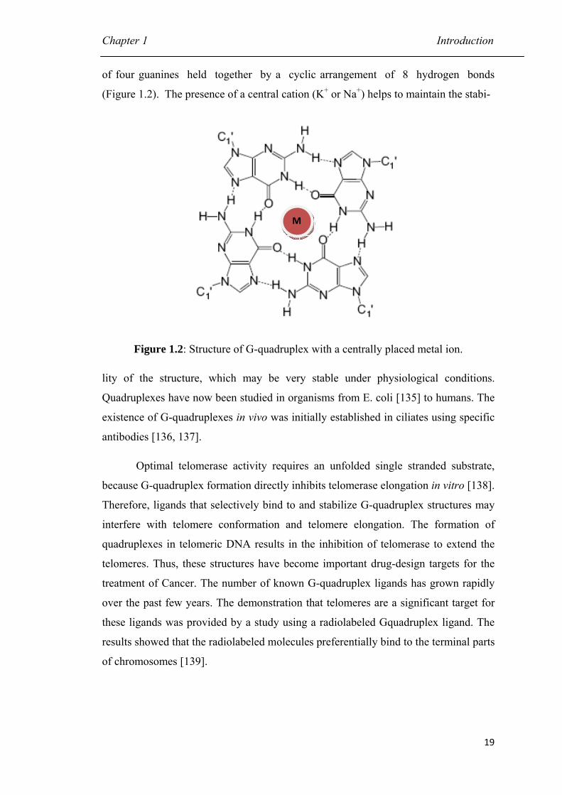
of four guanines held together by a cyclic arrangement of 8 hydrogen bonds

(Figure 1.2). The presence of a central cation (K+ or Na+) helps to maintain the stabi-

Figure 1.2: Structure of G-quadruplex with a centrally placed metal ion.

lity of the structure, which may be very stable under physiological conditions.

Quadruplexes have now been studied in organisms from E. coli [135] to humans. The

existence of G-quadruplexes in vivo was initially established in ciliates using specific

antibodies [136, 137].

Optimal telomerase activity requires an unfolded single stranded substrate,

because G-quadruplex formation directly inhibits telomerase elongation in vitro [138].

Therefore, ligands that selectively bind to and stabilize G-quadruplex structures may

interfere with telomere conformation and telomere elongation. The formation of

quadruplexes in telomeric DNA results in the inhibition of telomerase to extend the

telomeres. Thus, these structures have become important drug-design targets for the

treatment of Cancer. The number of known G-quadruplex ligands has grown rapidly

over the past few years. The demonstration that telomeres are a significant target for

these ligands was provided by a study using a radiolabeled Gquadruplex ligand. The

results showed that the radiolabeled molecules preferentially bind to the terminal parts

of chromosomes [139].

M


20

1.2.5 Structure and Topology of G-quadruplex

DNA is considered to be an important drug target in anticancer therapies.

Conventionally, the development of alkylating agents as anticancer agents is highly

dependent on the discovery and evolution of the DNA duplex and its associated

processes. Unfortunately, these drugs have drawbacks like extreme cytotoxicity and

nonspecificity. To solve these problems extensive efforts have been directed toward

the discovery of new agents with improved selectivity and lesser cytotoxicity [140].

Other than the typical double helix DNA proposed by Watson and Crick, DNA can

self-associate into other biologically relevant structures, known as G-quadruplexes.

This secondary DNA structure represents a new drug target for DNA-binding

compounds.

1.2.5.1 The building blocks of G-quadruplexes

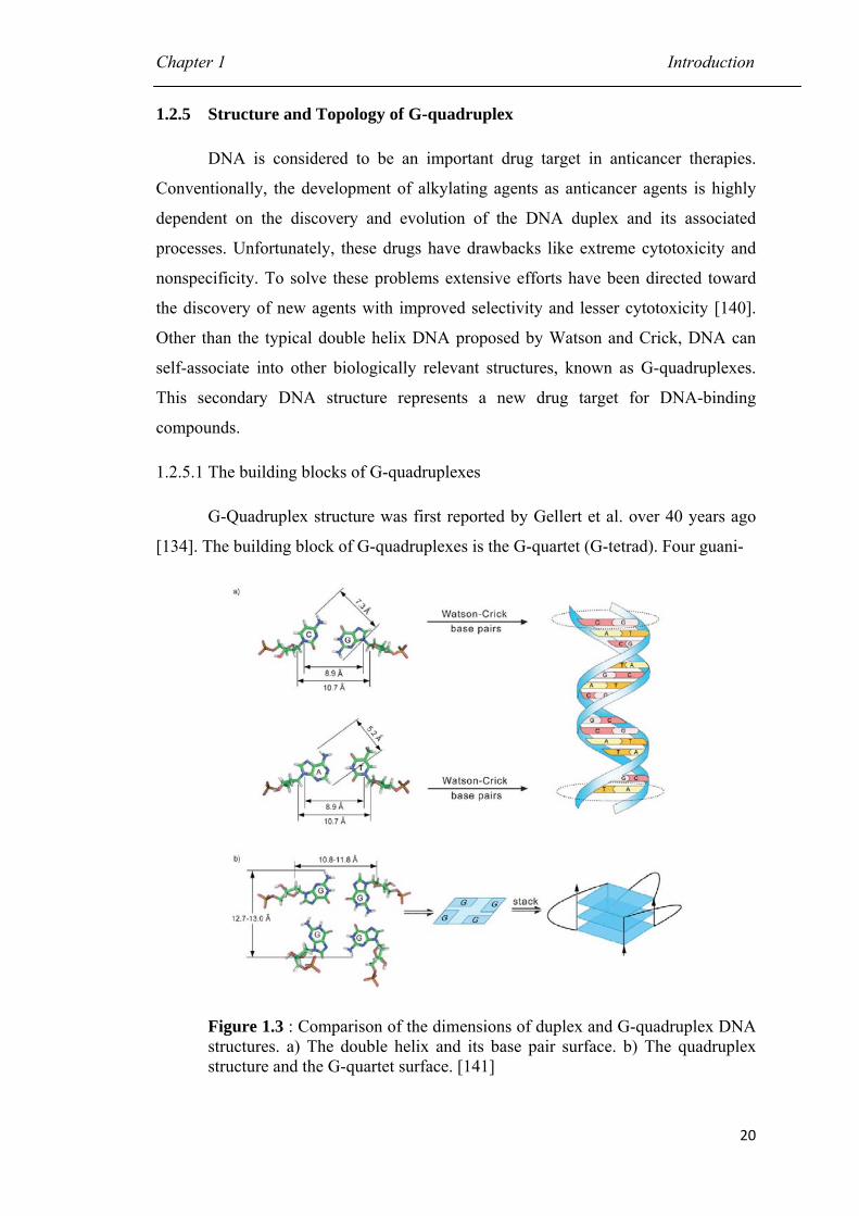
G-Quadruplex structure was first reported by Gellert et al. over 40 years ago

[134]. The building block of G-quadruplexes is the G-quartet (G-tetrad). Four guani-

Figure 1.3 : Comparison of the dimensions of duplex and G-quadruplex DNA structures. a) The double helix and its base pair surface. b) The quadruplex structure and the G-quartet surface. [141]


21

nes are associated into a cyclic Hoogsteen hydrogen bonding motif in which each

guanine base forms two hydrogen bonds with its neighbors as shown in Figure 1.3.

The advent of availability of crystal structures of G-quadruplex has shown that

the G-quartet has a square aromatic surface, the dimensions of which are much bigger

than the Watson-Crick base pairs (Figure 1.3) and this difference constitutes the basis

for designing G-quadruplex specific ligands [142, 143].

1.2.5.2 The basic topology and structure of G-quadruplexes

G-Quadruplex structures exhibit extensive structural diversity and

polymorphism. The structural polymorphism occurs mostly from the nature of the

loop, such as variations of strand stoichiometry, strand polarity, glycosidic torsion

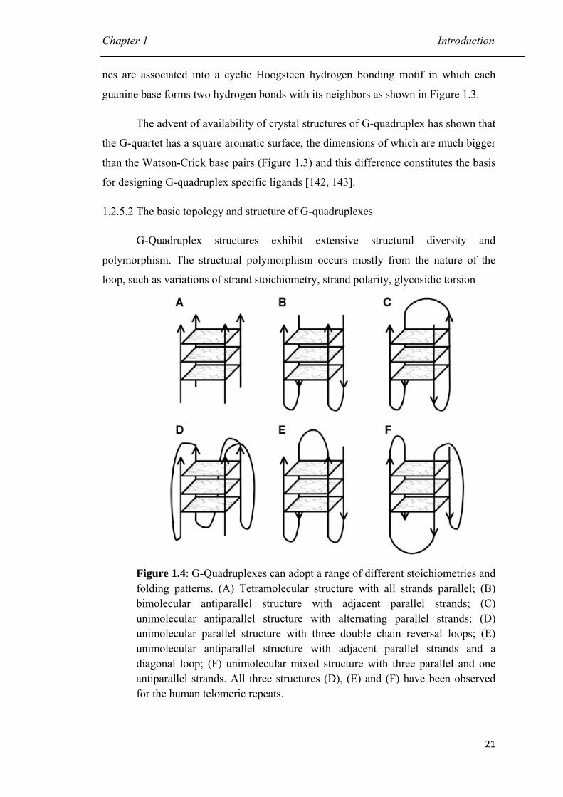
Figure 1.4: G-Quadruplexes can adopt a range of different stoichiometries and folding patterns. (A) Tetramolecular structure with all strands parallel; (B) bimolecular antiparallel structure with adjacent parallel strands; (C) unimolecular antiparallel structure with alternating parallel strands; (D) unimolecular parallel structure with three double chain reversal loops; (E) unimolecular antiparallel structure with adjacent parallel strands and a diagonal loop; (F) unimolecular mixed structure with three parallel and one antiparallel strands. All three structures (D), (E) and (F) have been observed for the human telomeric repeats.


22

angle and the location of the loops that link the guanine strands. Due to presence of

directionality to the strands, from the 5´ end to the 3´ end, there are topological

variants possible for these four strands. All four strands may be parallel, three parallel

and one in the opposite direction (antiparallel), or there may be two in one direction

and two in the other, either with the parallel pairs adjacent to each other or opposite to

each other. Some examples of different stoichiometries and folding patterns are

shown in Figure 1.4.

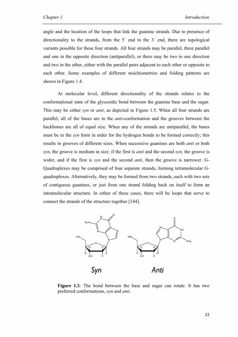
At molecular level, different directionality of the strands relates to the

conformational state of the glycosidic bond between the guanine base and the sugar.

This may be either syn or anti, as depicted in Figure 1.5. When all four strands are

parallel, all of the bases are in the anti-conformation and the grooves between the

backbones are all of equal size. When any of the strands are antiparallel, the bases

must be in the syn form in order for the hydrogen bonds to be formed correctly; this

results in grooves of different sizes. When successive guanines are both anti or both

syn, the groove is medium in size; if the first is anti and the second syn, the groove is

wider, and if the first is syn and the second anti, then the groove is narrower. G-

Quadruplexes may be comprised of four separate strands, forming tetramolecular G-

quadruplexes. Alternatively, they may be formed from two strands, each with two sets

of contiguous guanines, or just from one strand folding back on itself to form an

intramolecular structure. In either of these cases, there will be loops that serve to

connect the strands of the structure together [144].

Figure 1.5: The bond between the base and sugar can rotate. It has two preferred conformations, syn and anti.


23

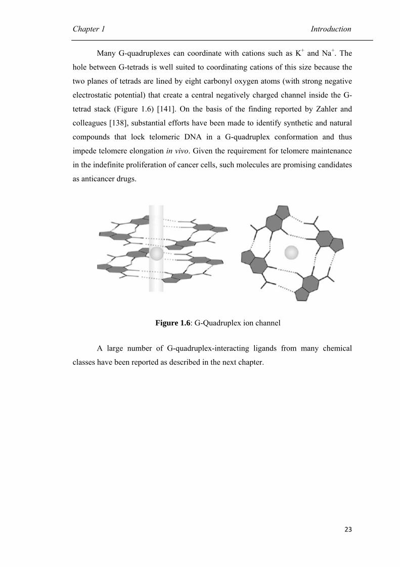
Many G-quadruplexes can coordinate with cations such as K+ and Na+. The

hole between G-tetrads is well suited to coordinating cations of this size because the

two planes of tetrads are lined by eight carbonyl oxygen atoms (with strong negative

electrostatic potential) that create a central negatively charged channel inside the G-

tetrad stack (Figure 1.6) [141]. On the basis of the finding reported by Zahler and

colleagues [138], substantial efforts have been made to identify synthetic and natural

compounds that lock telomeric DNA in a G-quadruplex conformation and thus

impede telomere elongation in vivo. Given the requirement for telomere maintenance

in the indefinite proliferation of cancer cells, such molecules are promising candidates

as anticancer drugs.

Figure 1.6: G-Quadruplex ion channel

A large number of G-quadruplex-interacting ligands from many chemical

classes have been reported as described in the next chapter.

1. introduction molecular modeling & drug...

Documents