1

Distributed Redundant Placement forMicroservice-based Applications at the Edge

Hailiang Zhao, Shuiguang Deng, Senior Member, IEEE, Zijie Liu, Jianwei Yin,and Schahram Dustdar, Fellow, IEEE

Abstract—Multi-access Edge Computing (MEC) is booming as a promising paradigm to push the computation and communicationresources from cloud to the network edge to provide services and to perform computations. With container technologies, mobiledevices with small memory footprint can run composite microservice-based applications without time-consuming backbone. Serviceplacement at the edge is of importance to put MEC from theory into practice. However, current state-of-the-art research does notsufficiently take the composite property of services into consideration. Besides, although Kubernetes has certain abilities to healcontainer failures, high availability cannot be ensured due to heterogeneity and variability of edge sites. To deal with these problems,we propose a distributed redundant placement framework SAA-RP and a GA-based Server Selection (GASS) algorithm formicroservice-based applications with sequential combinatorial structure. We formulate a stochastic optimization problem with theuncertainty of microservice request considered, and then decide for each microservice, how it should be deployed and with how manyinstances as well as on which edge sites to place them. Benchmark policies are implemented in two scenarios, where redundancy isallowed and not, respectively. Numerical results based on a real-world dataset verify that GASS significantly outperforms all thebenchmark policies.

Index Terms—Redundancy, Service Placement, Multi-access Edge Computing, Composite Service, Sample Average Approximation.

F

1 INTRODUCTION

NOWADAYS, mobile applications are becoming moreand more computation-intensive, location-aware, and

delay-sensitive, which puts a great pressure on the tradi-tional Cloud Computing paradigm to guarantee the Qualityof Service (QoS). To address the challenge, Multi-accessEdge Computing (MEC) was proposed to provide servicesand to perform computations at the network edge withouttime-consuming backbone transmission, so as to enable fastresponses for mobile devices [1] [2] [3].

MEC offers not only the development on the networkarchitecture, but also the innovation in service patterns.Considering that small-scale data-centers can be deployednear cellular tower sites, there are exciting possibilities thatmicroservice-based applications can be delivered to mobiledevices without backbone transmission, in virtue of settingup a unified service provision platform. Container technolo-gies, represented by Docker [4], and its dominant orchestra-tion and maintenance tool, Kubernetes [5], are becoming themainstream solution for packaging, deploying, maintaining,and healing applications. Each microservice decoupled fromthe application can be packaged as a Docker image and eachmicroservice instance is a Docker container. Here we takeKubernetes for example. Kubernetes is naturally suitable forbuilding cloud-native applications by leveraging the benefitsof the distributed edge because it can hide the complexity ofmicroservice orchestration while managing their availability

• H. Zhao, S. Deng, Z. Liu, and J. Yin are with the College of ComputerScience and Technology, Zhejiang University, Hangzhou 310058, China.E-mail: {hliangzhao, dengsg, liuzijie, zjuyjw}@zju.edu.cn

• S. Dustdar is with the Distributed Systems Group, Technische UniversitatWien, 1040 Vienna, Austria.E-mail: dustdar@dsg.tuwien.ac.at

• Shuiguang Deng is the corresponding author.

with lightweight Virtual Machines (VMs), which greatly mo-tivates Application Service Providers (ASPs) to participatein service provision within the access and core networks.

Service deployment from ASPs is the carrier of serviceprovision, which touches on where to place the services andhow to deploy their instances. In the last two years, thereexist works study the placement at the network edge fromthe perspective of Quality of Experience (QoE) of end usersor the budget of ASPs [6] [7] [8] [9] [10] [11] [12]. However,those works commonly have two limitations. Firstly, the to-be-deployed service only be studied in an atomic way. It isoften treated as a single abstract function with given inputand output data size. Time series or composition propertyof services are not fully taken into consideration. Secondly,high availability of deployed service is not carefully studied.Due to the heterogeneity of edge sites, such as different CPUcycle frequency and memory footprint, varying backgroundload, transient network interrupts and so on, the serviceprovision platform might face greatly slowdowns or evenruntime crash. However, the default assignment, deploy-ment, and management of containers does not fully take theheterogeneity in both physical and virtualized nodes intoconsideration. Besides, the healing capability of Kubernetesis principally monitoring the status of containers, pods,and nodes and timely restarting the failures, which is notenough for high availability. Vayghan et al. find that in thespecific test environment, when the pod failure happens, theoutage time of the corresponding service could be dozensof seconds. When node failure happens, the outage timecould be dozens of minutes [13] [14]. Therefore, with thevanilla version of Kubernetes, high availability might notbe ensured, especially for the latency-critical cloud-nativeapplications. Besides, one microservice could have several

2

alternative execution solutions. For example, electronic pay-ment, as a microservice of a composite service, can beexecuted by PayPal, WeChat Pay, and AliPay1. In this paper,let us call them candidates (of microservices). This status quocomplicates the placement problem further. Because it is theinstances of candidates that need to be placed, which greatlyscales up the problem.

In order to solve the above problems, we propose a dis-tributed redundant placement framework, i.e., Sample Av-erage Approximation-based Redundancy Placement (SAA-RP), for a microservice-based applications with sequentialcombinatorial structure. For this application, if all of thecandidates are placed on one edge site, network congestionis inevitable. Therefore, we adopt a distributed placementscheme, which is naturally suitable for the distributed edge.Redundancy is the core of SAA-RP, which allows that onecandidate to be dispatched to multiple edge sites. By creat-ing multiple candidate instances, it boosts a faster responseto service requests. To be specific, it alleviates the risk of along delay incurred when a candidate is assigned to onlyone edge site. With one candidate deployed on more thanone edge site, requests from different end users at differentlocations can be balanced, so as to ensure the high availabil-ity of service and the robustness of the provision platform.Actually, performance of redundancy has been extensivelystudied under various system models and assumptions,such as the Redundancy-d model, the (n, k) system, andthe S&X model [15]. However, which kind of candidaterequires redundancy and how many instances should bedeployed cannot be decided if out of a concrete situation.Currently, the main strategy of job redundancy usuallyreleases the resource occupancy after completion, whichis not befitting for geographically distributed edge sites.This is because service requests are continuously gener-ated from different end users. The destruction of candidateinstances have to be created again, which will certainlylead to the delay in service responses. Besides, redundancyis not always a win and might be dangerous sometimes,since practical studies have shown that creating too manyinstances can lead to unacceptably high response times andeven instability [15].

As a result, we do not release the candidate instancesbut periodically update them based on the observations ofservice demand status during that period. Specifically, wederive expressions to decide each candidate should be dis-patched with how many instances and which edge sites toplace them. By collecting user requests for different servicecomposition schemes, we model the distributed redundantplacement as a stochastic discrete optimization problemand approximate the expected value through Monte Carlosampling. During each sampling, we solve the determinis-tic problem based on an efficient evolutionary algorithm.Performance analysis and numerical results are providedto verify its practicability. Our main contributions are asfollows.

1) We model the distributed placement scenario at theedge for general microservice-based chained appli-cations and design a distributed redundant place-

1. Both Alipay and WeChat Pay are third-party mobile and onlinepayment platforms, established in China.

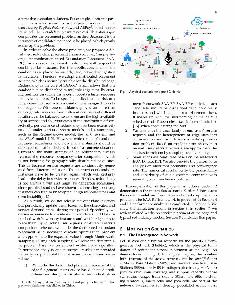
Fig. 1. A typical scenario for a pre-5G HetNet.

ment framework SAA-RP. SAA-RP can decide eachcandidate should be dispatched with how manyinstances and which edge sites to placement them.It makes up with the shortcoming of the defaultscheduler of Kubernetes, i.e. kube-scheduler[16], when encountering the MEC.

2) We take both the uncertainty of end users’ servicerequests and the heterogeneity of edge sites intoconsideration and formulate a stochastic optimiza-tion problem. Based on the long-term observationon end users’ service requests, we approximate thestochastic problem by sampling and averaging.

3) Simulations are conducted based on the real-worldEUA Dataset [17]. We also provide the performanceanalysis on algorithm optimality and convergencerate. The numerical results verify the practicabilityand superiority of our algorithm, compared withseveral typical benchmark policies.

The organization of this paper is as follows. Section 2demonstrates the motivation scenario. Section 3 introducesthe system model and formulates a stochastic optimizationproblem. The SAA-RP framework is proposed in Section 4and its performance analysis is conducted in Section 5. Weshow the simulation results in Section 6. In Section 7, wereview related works on service placement at the edge andtypical redundancy models. Section 8 concludes this paper.

2 MOTIVATION SCENARIOS

2.1 The Heterogeneous Network

Let us consider a typical scenario for the pre-5G Hetero-geneous Network (HetNet), which is the physical foun-dation of redundant service placement at the edge. Asdemonstrated in Fig. 1, for a given region, the wirelessinfrastructure of the access network can be simplified intoa Macro Base Station (MBS) and several Small-cell BaseStations (SBSs). The MBS is indispensable in any HetNet toprovide ubiquitous coverage and support capacity, whosecell radius ranges from 8km to 30km. The SBSs, includ-ing femtocells, micro cells, and pico cells, are part of thenetwork densification for densely populated urban areas.

3

Without loss of generality, WiFi access points, routers, andgateways are viewed as SBSs for simplification. Their cellradius ranges from 0.01km to 2km. The SBSs can be logicallyinterconnected to transfer signaling, broadcast message, andselect routes. It might be too luxurious if all SBSs are fullyinterconnected, and not necessarily achievable if they areset up by different Mobile Telecom Carriers (MTCs)2, butwe reasonably assume that each SBS is mutually reachableto formulate an undirected connected graph. This can be seenin Fig. 1. Each SBS has a corresponding small-scale data-center attached for the deployment of microservices and theallocating of resources.

In this scenario, end users with their mobile devices canmove arbitrarily within a certain range. For example, endusers work within a building or rest at home. In this case,the connected SBS of each end user does not change.

2.2 Response Time of MicroservicesA microservice-based application consists of multiple mi-croservices. Each microservice can be executed by manyavailable candidates. Take an arbitrary e-commerce appli-cation as an example. When we shop on a client browser,we firstly search the items we want, which can be real-ized by many site search APIs. Secondly, we add themto the cart and pay for them. The electronic payment canbe accomplished by Alipay, WeChat Pay, or PayPal byinvoking their APIs. After that, we can review and rate forthose purchased items. In this example, each microserviceis focused on single business capability. In addition, theconsidered application might have complex compositionalstructures and complex correlations between the fore-and-aft candidates because of bundle sales. For example, whenwe are shopping on Taobao3, only Alipay is supported foronline payment. The application in the above example hasa linear structure. As a beginning, this paper only caresabout the sequentially composed application. In practice, ageneral directed acyclic graph (DAG) can be decomposedinto several linear chains by applying Flow DecompositionTheorem (located in Chapter 03) [18]. We leave the extensionto future work.

The pre-5G HetNet allows SBSs to share a mobile serviceprovision platform, where user configurations and contex-tual information can be uniformly managed. As we havementioned before, the unified platform can be implementedby Kubernetes. In our scenario, each mobile device sendsits service request to the nearest SBS for the strongestsignal of the established link. However, if there are no SBSsaccessible, the request has to be responded by the MBS andprocessed by cloud data-centers. All the possibilities of theresponse status of the first microservice is discussed below.

1) The requested candidate is deployed at the chosenSBS. It will be processed by this SBS instantly.

2) The requested candidate is not deployed at thenearest SBS but accessible on other SBSs, whichleads to multi-hop transfers between the SBSs untilthe request is responded by another SBS. That is,

2. Whether SBSs are logically connected comes down to their IPsegments.

3. Taobao is the world’s biggest e-commerce website, established inChina.

App with 4 microservices

: the 1st composite scheme

: the 2nd composite scheme

m1 m2 m3 m4

c11

c12

c21

c31

c32

c41

c42

Fig. 2. Two service composition schemes for a 4-microservice app.

1 2

2 4 3

3 1

4c11

SBS 1

SBS 2

SBS 3

SBS 4

SBS 5

SBS 6

c12

c12

c31

c32

c32

c42

c41

c21MD 1

MD 2

c21

Fig. 3. The placement of each candidates on the HetNet.

the request will route through the HetNet until itis responded by an SBS who deploys the requiredcandidate.

3) The requested candidate is not deployed on anySBSs in the HetNet. It can only be processed bycloud through backbone transmission.

For the subsequent microservices, the response statusalso faces many possibilities:

1) The previous candidate is processed by an SBS.Under this circumstance, for candidate of this mi-croservice, if its instance can be found in the HetNet,multi-hop transfer is required. Otherwise, it has tobe processed by cloud.

2) The previous candidate is processed by cloud. Un-der this circumstance, the candidates of subsequentmicroservices should always be responded by cloudwithout unnecessary backhaul.

Our job is to find an optimal redundant placement policywith the trade-offs between resource occupation and re-sponse time considered. We should know which candidateswho might as well be redundant and where to deploy them.

2.3 A Working ExampleThis subsection describes a small-scale working example.

Microservices and Candidates: Fig. 2 demonstrates achained application constitutive of four microservices. Eachmicroservice has 2, 1, 2, and 2 candidates, respectively. Thefirst service composition scheme is c11 → c21 → c31 → c42,and the second service composition scheme is c12 → c21 →c32 → c41. In practice, the composition scheme is decidedby the daily usage habits of end users. It might be strongly

4

biased. Besides, because of bundle sales, part of the compo-sition might be fixed. We will describe the composition interms of a joint probability distribution in Subsection 3.1.

Service Placement of Instances: In Fig. 3, the undirectedconnected graph consists of 6 SBSs. The number taggedinside each SBS is its maximum number of placeable can-didates. For example, SBS2 can be placed at most 4 can-didates. This constraint exists because the edge sites havevery limited computation and storage resources, comparedwith cloud data-centers. The squares beside each SBS arethe deployed candidates. For example, SBS1 deploys twocandidates, c11 and c21. Notice that because of the redun-dancy mechanism, the same candidate can be deployed onmultiple SBSs. For example, c21 is dispatched to both SBS1and SBS2.

Fig. 3 also demonstrates two mobile devices, MD1 andMD2, which are located beside SBS1 and SBS5, respectively.It means that the SBSs closest to MD1 and MD2 are SBS1and SBS5, respectively. As we have already mentioned inSubsection 2.2, the service request of each mobile device isresponded by the nearest SBS. Thus, for MD1 and MD2,SBS1 and SBS5 are the corresponding SBS for responding,respectively.

Response Time Calculation: We assume that the servicecomposition scheme of MD1 is the red one in Fig. 2, andMD2’s is the blue one. The number tagged inside eachcandidate is the executing sequence. Let us take a closerlook at MD1.

1) c11: Because c11 is deployed on SBS1, the responsetime of c11 is equal to the sum of the expenditure oftime on wireless access between MD1 and SBS1 andthe processing time of c11 on SBS1.

2) c21: Because c21 can also be found on SBS1, theexpenditure time is zero. The response time of c21consists of only the processing time of c21 on SBS1.

3) c31: c31 can only be found on SBS2, thus the ex-penditure time of it is equal to the routing timefrom SBS1 to SBS2. In this paper, we assume thatthe routing between two nodes always selects thenearest path in the undirected graph. Thus, only onehop is required (SBS1 → SBS2). Thus, the responsetime of c31 consists of the routing time from SBS1 toSBS2 and the processing time of c31 on SBS2.

4) c42: c42 can only be found on SBS6. Thus, the ex-penditure requires 2 hops (SBS2 → SBS4 → SBS6or SBS2→ SBS5→ SBS6). Finally, the output of c42need to be transferred back to MD1 via SBS1. Thenearest path from SBS6 to SBS1 requires 3 hops.There are three alternatives: (i) SBS6 → SBS4 →SBS2→ SBS1 or (ii) SBS6→ SBS5→ SBS2→ SBS1or (iii) SBS6 → SBS5 → SBS3 → SBS1. Thus, theresponse time of c42 consists of the routing timefrom SBS2 to SBS6, the processing time of c42 onSBS6, the routing time from SBS6 to SBS1, and thewireless transmission time from SBS1 to MD1.

The response time of the 1st composition scheme is thesum of the response time of c11, c21, c31, and c42. Thesame procedure applies to MD2. In addition, there are twounexpected cases need to be addressed. The first one is thatif a mobile device is covered by no SBS, the response should

TABLE 1Summary of key notations.

Notation Description

M the number of SBSs, M = |M|N the number of mobile devices, N = |N |

Qthe number of microservices in the application,Q = |Q|

tq , q ∈ Q the qth microservice in the application

Mithe set of SBSs that can be connected by theith mobile device

Njthe set of mobile devices that can be

connected by the jth SBS

Cqthe number of candidates of the qth

microservice, Cq = |Cq |, q ∈ Qscq , c ∈ Cq the cth candidate of the qth microserviceD(scq) the set of SBSs on which scq is deployed

E(scq)the random event that for microservice tq , the cth

candidate is selected for executionj?i the nearest SBS to the ith mobile devicejp(scq) the SBS who actually processes the candidate scq

d(i, j)the Euclidean distance between the ith mobile

device and the jth SBS

τin(scq)

the data uplink transmission time of thecandidate scq

τexe(jp(scq))the execution time of the candidate scq on

the jpth SBS

ζ(j1, j2)the hop-count between the j1th SBS

and the j2th SBS

bjthe maximum number of microservice instances

can be deployed on the jth SBS

be made by the MBS and all the microservices are processedby cloud. The second one is that if a required candidate isnot deployed on any SBS, then a communication link fromthe SBS processing the last candidate to the cloud should beestablished. This candidate and all the candidates of the restmicroservices will be processed on cloud. The response timeis calculated in a different way for these cases. Nevertheless,all the contingencies are taken into account in our systemmodel, elaborated in Section 3.

Obviously, a better service placement policy can leadto less time spent. Our job is to find a service placementpolicy to minimize the response time of all mobile devices.What need to determine are not only how many instancesrequired for each candidate, but also which edge sites toplace them. The next section will demonstrate the rigorousformulation of system model.

3 SYSTEM MODEL

The HetNet consists of N mobile devices, indexed by N ,{1, ..., i, ..., N}, M SBSs, indexed by M , {1, ..., j, ...,M},and one MBS, indexed by 0. Considering that each mobiledevice might be covered by many SBSs, let us use Mi todenote the set of SBSs whose wireless signal covers theith mobile devices. Correspondingly, Nj denotes the set ofmobile devices that are covered by the jth SBS. Notice thatthe service request from a mobile device is responded byits nearest available SBS, otherwise the MBS. The MBS hereis to provide ubiquitous signal coverage and is always con-nectable to each mobile device. Both the SBSs and the MBSare connected to the backbone. Table 1 lists key notations inthis paper.

5

3.1 Describing the Correlated MicroservicesWe consider an application with Q sequential compositemicroservices 〈t1, ..., tQ〉, indexed by Q. ∀q ∈ Q, microser-vice tq has Cq candidates {s1q, ..., scq, ..., s

Cqq }, indexed by

Cq . Let us use D(scq) ⊆ M to denote the set of SBSs onwhich scq is deployed. Our redundancy mechanism allowsthat |D(scq)| > 1, which means one candidate instance couldbe dispatched to more than one SBS. Besides, let us useE(scq), c ∈ Cq to represent that for microservice tq , the cthcandidate is selected for execution. E(scq) can be viewedas a random event with an unknown distribution. Further,P(E(scq)) denote the probability that E(scq) happens. Thus,for each mobile device, its selected candidates can be de-scribed as a Q-tuple:

(s) , 〈E(sc11 ), ..., E(scQQ )〉, (1)

where q ∈ Q, cq ∈ Cq .The sequential composite application might have corre-

lations between the fore-and-aft candidates. The definitionbelow gives a rigorous mathematical description.Definition 3.1. Correlations of Composite Service ∀q ∈Q\{1}, c1 ∈ Cq−1, and c2 ∈ Cq , candidate sc2q andsc1q−1 are correlated iff P(E(sc2q )|E(sc1q−1)) ≡ 1, and

∀c′2 ∈ Cq\{c2}, P(E(sc′2q )|E(sc1q−1)) ≡ 0.

With the above definition, the probability P(E(s)) can becalculated by

P(E(s)) =

P(E(sc11 )) ·Q∏

q=2

P(E(scqq )|E(scq−1

q−1 )). (2)

3.2 Calculating the Respone TimeThe response time of one candidate consists of data uplinktransmission time, service execution time, and data down-link transmission time. The data uploaded is mainly en-coded service requests and configurations while the outputis mainly the feedback on successful service execution ora request to invoke the next candidate. If all requests areresponded within the access network, most of the time isspent on routing with multi-hops between SBSs. Notice thatexcept the last one, each candidate’s data uplink transmis-sion time is equal to the data downlink transmission time ofthe candidate of its previous microservice.

3.2.1 For the Initial CandidateFor the ith mobile device and its selected candidate sc11 (i) ofthe initial microservice t1, where c1 ∈ C1, (I) if the ith mobiledevice is not covered by any SBSs around, i.e.,Mi = ∅, therequest has to be responded by the MBS and processed bycloud data-center. (II) If Mi 6= ∅, as we have mentionedbefore, the nearest SBS j?i ∈ Mi is chosen and connected.Under this circumstance, a classified discussion is required.

1) If the candidate sc11 (i) is not deployed on any SBSsfrom M, i.e. D(sc11 (i)) = ∅, the request still hasto be forwarded to cloud data-center through back-bone transmission.

2) If D(sc11 (i)) 6= ∅ and j?i ∈ D(sc11 (i)), the request canbe directly processed by SBS j?i without any hops.

3) If D(sc11 (i)) 6= ∅ and j?i /∈ D(sc11 (i)), the request hasto be responded by j?i and processed by another SBSfrom D(sc11 (i)).

We use jp(s) to denote the SBS who actually processess. Remember that the routing between two nodes alwaysselects the nearest path. Thus, for q = 1, jp(s

c11 (i)) can be

obatined by (3), where ζ(j1, j2) is the shortest number ofhops from node j1 to node j2.

In this paragragh, we calculate the response time ofsc11 (i). We use d(i, j) to denote the reciprocal of the band-width between i and j. Obviously, the expenditure of timeon wireless access is inversely proportional to the band-width of the link. Besides, the expenditure of time on rout-ing is directly proportional to the number of hops betweenthe source node and destination node. As a result, the datauplink transmission time τin(sc11 (i)) is summarized in (4),where τb is the time on backbone transmission, α is sizeof input data stream from each mobile device to the initialcandidate (measured in bits), and β is a positive constantrepresenting the rate of wired link between SBSs. We useτexe(jp(s

c11 (i))) to denote the microservice execution time

on the SBS jp for the candidate sc11 (i). The data downlinktransmission time is the same as the uplink time of the nextmicroservice, which is discussed hereinafter.

3.2.2 For the Intermediate Candidates

For the ith mobile device and its selected candidate scqq (i)of microservice tq , where q ∈ Q\{1, Q}, cq ∈ Cq , theanalysis of its data uplink transmission time is correlatedwith jp(s

cq−1

q−1 (i)), i.e. the SBS who processes scq−1

q−1 (i). ∀q ∈Q\{1}, the calculation of jp(s

cqq (i)) is summarized in (5).

This formula is closely related to (3).In this paragragh, we calculate the response time of

scqq (i). (I) If jp(s

cq−1

q−1 (i)) ∈ D(scqq (i)), then the data downlink

transmission time of previous candidate scq−1

q−1 (i), which isalso the data uplink transmission time of current candidatescqq (i), is zero. That is, τout(s

cq−1

q−1 (i)) = τin(scqq (i)) = 0. It

is because both scq−1

q−1 (i) and scqq (i) are deployed on the SBSjp(s

cq−1

q−1 (i)), which leads to the number of hops being zero.(II) If jp(s

cq−1

q−1 (i)) /∈ D(scqq (i)), a classified discussion has to

be launched.

1) If jp(scq−1

q−1 (i)) = cloud, which means the requestof tq−1 from the ith mobile device is respondedby cloud data-center. In this case, the invocationfor tq can be directly processed by cloud withoutbackhaul. Thus, the data uplink transmission timeof tq is zero, too.

2) If jp(scq−1

q−1 (i)) 6= 0 and D(scqq (i)) = ∅, which means

scqq (i) is not deployed on any SBSs in the HetNet. As

a result, the invocation for tq has to be responded bycloud data-center through backbone transmission.

3) If jp(scq−1

q−1 (i)) 6= 0, D(scqq (i)) 6= ∅ but jp(s

cq−1

q−1 (i)) /∈D(s

cqq (i)), which means both scq−1

q−1 (i) and scqq (i) areprocessed by the SBSs in the HetNet but not thesame one. In this case, we can calculate the datauplink transmission time by finding the shortestpath from jp(s

cq−1

q−1 (i)) to a SBS in D(scqq (i)).

The above analysis is summarized in (6).

6

jp(sc11 (i)) =

cloud, Mi = ∅ or D(sc11 (i)) = ∅;j?i , D(sc11 (i)) 6= ∅, j?i ∈ D(sc11 (i));argminj•∈D(s

c11 (i)) ζ(j?i , j

•), otherwise(3)

τin(sc11 (i)) =

α · d(i, 0) + τb, Mi = ∅;α · d(i, j?i ) + τb, Mi 6= ∅,D(sc11 (i)) = ∅;α · d(i, j?i ), Mi 6= ∅, j?i ∈ D(sc11 (i));α · d(i, j?i ) + β ·minj•∈D(s

c11 (i)) ζ(j?i , j

•), otherwise

(4)

jp(scqq (i)) =

cloud, Mi = ∅ or D(scqq (i)) = ∅;

jp(scq−1

q−1 (i)), D(scqq (i)) 6= ∅, jp(s

cq−1

q−1 (i)) ∈ D(scqq (i));

argminj•∈D(scqq (i)) ζ(jp(s

cq−1

q−1 (i)), j•), otherwise(5)

τin(scqq (i)) =

0, jp(scq−1

q−1 (i)) ∈ D(scqq (i)) or jp(s

cq−1

q−1 (i)) = cloud;τb, jp(s

cq−1

q−1 (i)) 6= 0,D(scqq (i)) = ∅;

β ·minj•∈D(scqq (i)) ζ(jp(s

cq−1

q−1 (i))), j•), otherwise(6)

τout(scQQ (i)) =

{τb + α · d(i, 0), jp(s

cQQ (i)) = cloud;

β · ζ(jp(scQQ (i)), j?i ) + α · d(i, j?i ), otherwise

(7)

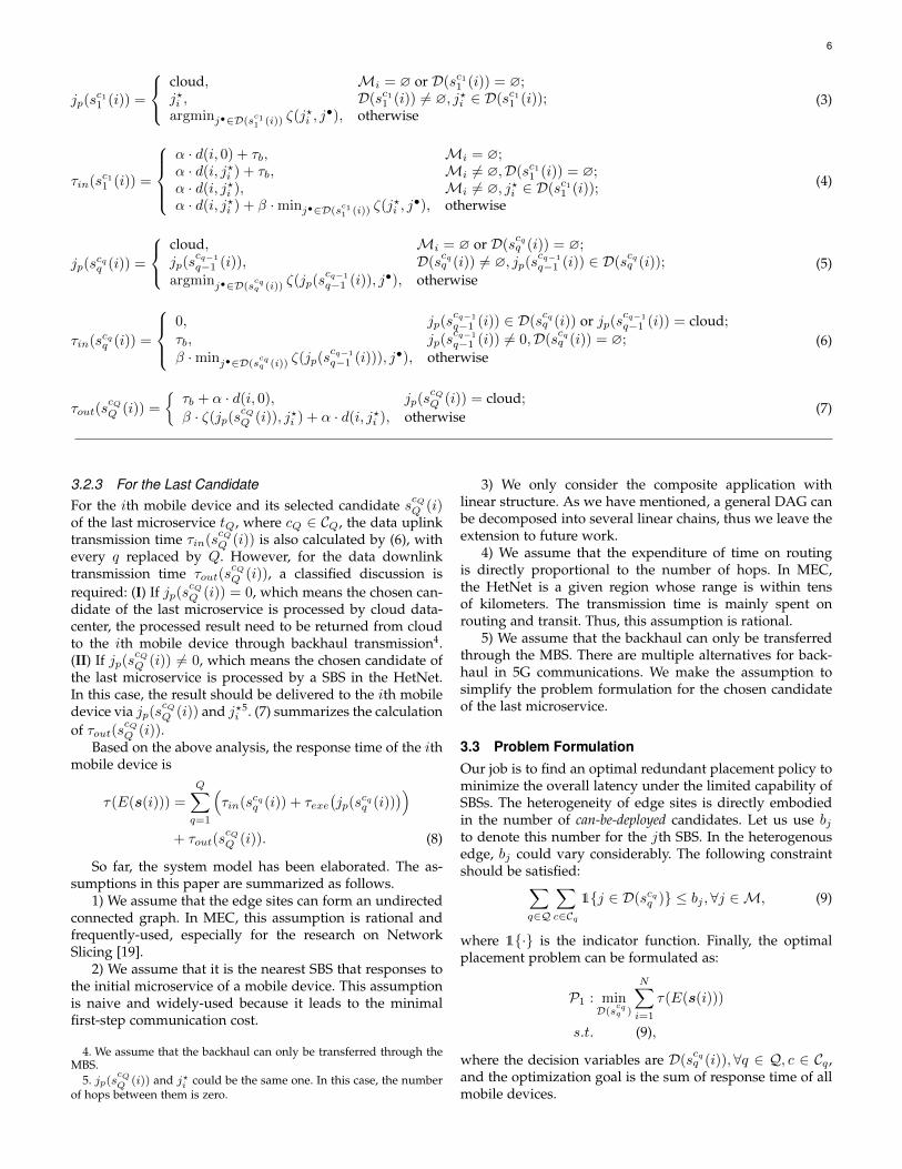
3.2.3 For the Last CandidateFor the ith mobile device and its selected candidate scQQ (i)of the last microservice tQ, where cQ ∈ CQ, the data uplinktransmission time τin(s

cQQ (i)) is also calculated by (6), with

every q replaced by Q. However, for the data downlinktransmission time τout(s

cQQ (i)), a classified discussion is

required: (I) If jp(scQQ (i)) = 0, which means the chosen can-

didate of the last microservice is processed by cloud data-center, the processed result need to be returned from cloudto the ith mobile device through backhaul transmission4.(II) If jp(s

cQQ (i)) 6= 0, which means the chosen candidate of

the last microservice is processed by a SBS in the HetNet.In this case, the result should be delivered to the ith mobiledevice via jp(s

cQQ (i)) and j?i

5. (7) summarizes the calculationof τout(s

cQQ (i)).

Based on the above analysis, the response time of the ithmobile device is

τ(E(s(i))) =

Q∑

q=1

(τin(scqq (i)) + τexe

(jp(s

cqq (i))

))

+ τout(scQQ (i)). (8)

So far, the system model has been elaborated. The as-sumptions in this paper are summarized as follows.

1) We assume that the edge sites can form an undirectedconnected graph. In MEC, this assumption is rational andfrequently-used, especially for the research on NetworkSlicing [19].

2) We assume that it is the nearest SBS that responses tothe initial microservice of a mobile device. This assumptionis naive and widely-used because it leads to the minimalfirst-step communication cost.

4. We assume that the backhaul can only be transferred through theMBS.

5. jp(scQQ (i)) and j?i could be the same one. In this case, the number

of hops between them is zero.

3) We only consider the composite application withlinear structure. As we have mentioned, a general DAG canbe decomposed into several linear chains, thus we leave theextension to future work.

4) We assume that the expenditure of time on routingis directly proportional to the number of hops. In MEC,the HetNet is a given region whose range is within tensof kilometers. The transmission time is mainly spent onrouting and transit. Thus, this assumption is rational.

5) We assume that the backhaul can only be transferredthrough the MBS. There are multiple alternatives for back-haul in 5G communications. We make the assumption tosimplify the problem formulation for the chosen candidateof the last microservice.

3.3 Problem FormulationOur job is to find an optimal redundant placement policy tominimize the overall latency under the limited capability ofSBSs. The heterogeneity of edge sites is directly embodiedin the number of can-be-deployed candidates. Let us use bjto denote this number for the jth SBS. In the heterogenousedge, bj could vary considerably. The following constraintshould be satisfied:

∑

q∈Q

∑

c∈Cq1{j ∈ D(scqq )} ≤ bj ,∀j ∈M, (9)

where 1{·} is the indicator function. Finally, the optimalplacement problem can be formulated as:

P1 : minD(s

cqq )

N∑

i=1

τ(E(s(i)))

s.t. (9),

where the decision variables are D(scqq (i)),∀q ∈ Q, c ∈ Cq ,

and the optimization goal is the sum of response time of allmobile devices.

7

4 ALGORITHM DESIGN

In this section, we elaborate our algorithm for P1. Firstly,we recode the decision variables as x to shrink the sizeof feasible region. Based on that, we propose the SAA-RP framework. It includes a subroutine, named GeneticAlgorithm-based Server Selection (GASS) algorithm. Thedetails are presented as follows.

4.1 Variable RecodingLet us use W (i) , (canIdx(t1), ...,canIdx(tQ)) to de-note the random vector on the chosen service compositionscheme of the ith mobile device, where canIdx(tq) returnsthe index of the chosen candidate of the qth microservice.W (i) and E(s(i)) describe the same thing from differentperspectives. However, the former is more concise. Then, weuse W , (W (1), ...,W (N)) to denote the global randomvector by taking all mobile devices into account. Let us usex , [x(b1), ...,x(bM )]> to recode the global deploy-or-notvector. ∀j ∈ M,x(bj) is a deployment vector for SBS j,whose length is bj . By doing this, the constraint (9) can beremoved because it is reflected in how x encodes. ∀j ∈ M,each element of x(bj) is chosen from {0, 1, ...,

∑q=1 Cq}, i.e.

the global index of each candidate. That is, any candidatecan appear in any number of SBSs in the HetNet. Thus, theredundancy mechanism is also reflected in how x encodes.∀j ∈ M, x(bj) = 0 means that the jth SBS does not deployany candidate.

x is a new encoding of D(scqq (i)). As a result, we can

reconstitute τ(E(s(i))) as τ(x,W (i)). As such, the opti-mization goal can be written as

g(x) , E[G(x,W )] = E[N∑

i=1

τ(x,W (i))], (10)

and the optimal placement problem is

P2 : minx∈X

g(x).

P2 is a stochastic discrete optimization problem with in-dependent variable x, where X is the feasible region. X ,although finite, is very large. Therefore, enumeration ap-proach is inadvisable. Besides, the problem has an uncertainrandom vector W with probability distribution P(E(s(i))).

4.2 The SAA-RP FrameworkLet us take a closer look at P2. Firstly, the random vectorW is exogenous because the decision on x does not affectthe distribution of W . Secondly, for a given W , G(x,W )can be easily evaluated for any x. Thus, the observationof G(x,W ) is constructive. As a result, we can apply theSample Average Approximation (SAA) approach to P1 [20]to handle with the uncertainty.

SAA is a classic Monte Carlo simulation-based method.In the following section, we elaborate how we apply theSAA method to P2. Formally, we define the SAA problemP3. Let W 1,W 2, ...,WR be an independently and identi-cally distributed (i.i.d.) random sample of R realizations ofthe random vector W . The SAA function is defined as

gR(x) ,1

R

R∑

r=1

G(x,W r), (11)

and the SAA problem P3 is defined as

P3 : minx∈X

gR(x).

By Monte Carlo Sampling, with support from the Law ofLarge Numbers [21], when R is large enough, the optimalvalue of gR(x) can converge to the optimal value of g(x)with probability one (w.p.1). As a result, we only need tocare about how to solve P3 as optimal as possible.

Algorithm 1 SAA-based Redundant Placement (SAA-RP)1: Choose initial sample size R and R′ (R′ � R)2: Choose the number of replications L (indexed by L)3: Set up a gap tolerance ε4: for l = 1 to L in parallel do5: Generate R independent samples W 1

l , ...,WRl

6: Call GASS to obtain the minimum value of gR(xl)with the form of 1

R

∑Rr=1G(xl,W

rl )

7: Record the optimal goal gR(x∗l ) and the correspond-ing variable x∗l returned from GASS

8: end for9: v∗R ← 1

L

∑Ll=1 gR(x∗l )

10: for l = 1 to L in parallel do11: Generate R′ independent samples W 1

l , ...,WR′

l

12: vlR′ ← 1R′∑R′

r′=1G(x∗l ,Wr′

l )13: end for14: Get the worst replication v•R′ ← maxl∈L vlR′15: if the gap v•R′ − v∗R < ε then16: Choose the best solution x∗l among all L replicationss17: else18: Increase R (for drill) and R′ (for evaluation)19: goto Step. 420: end if21: return the best solution x∗l

The SAA-RP framework is presented in Algorithm 1.Firstly, we need to select the sample size R and R′ ap-propriately. As the sample size R increases, the optimalsolution of the SAA problem P2 converges to its true problemP1. However, the computational complexity for solving P2

increases at least linearly, even exponentially, in the samplesize R [20]. Therefore, when we choose R, the trade-offbetween the quality of the optimality and the computationeffort should be taken into account. Besides, R′ here is usedto obtain an estimate of P1 with the obtained solution ofP2. In order to obtain an accurate estimate, we have everyreason to choose a relatively large sample size R′ (R′ � R).Secondlly, inspired by [20], we replicate generating andsolving P2 with L i.i.d. replications. From Step. 4 to Step.8, we call the algorithm GASS to obtain the asymptoticallyoptimal solution of P2 and record the best-so-far results.From Step. 10 to Step. 13, we estimate the true value of P1

for each replication. After that, those estimates are comparedwith the average of those optimal solutions of P2. If themaximum gap is smaller than the tolerance, SAA-RP returnsthe best solution among L replications and the algorithmterminates, otherwise we increase R and R′ and drill again.

4.3 The GASS AlgorithmGASS is implemented based on the well-konwn GeneticAlgorithm (GA). The detailed procedure is demonstrated in

8

Algorithm 2. Firstly, we initialize the necessary parameters,including the population size P , the number of iterationsit, and the probability of crossover Pc and mutation Pm,respectively. After that, we randomly generate the initialpopulation from the domain X . From Step. 6 to Step. 10,GASS executes the crossover operation. At the beginning ofthis operation, GASS checks whether crossover need to beexecuted. If yes, GASS choose the best two chromosomesaccording to their fitness values. With that, the latter part ofxp1 and xp2 are exchanged since the position x(bj). FromStep. 11 to Step. 13, GASS executes the mutation operation.At the beginning of this operation, it checks whether eachchromosome can mutate according to the mutation proba-bility Pm. At the end, only the chromosome with the bestfitness value can be returned.

Algorithm 2 GA-based Server Selection (GASS)1: Initialize the population size P , number of iterations it,

the probability of crossover Pc and mutation Pm2: Randomly generate P chromosomes x1, ...,xP ∈ X3: for t = 1 to it do4: ∀p ∈ {1, ..., P}, renew the optimization goal of P2, i.e.

gR(xp), according to (11)5: for p = 1 to P do6: if rand() < Pc then7: Choose two chromosomes p1 and p2 according to

the probability distribution:

P(p is chosen) =1/gR(xp)

∑Pp′=1 1/gR(xp′)

8: Randomly choose SBS j ∈M9: Crossover the segement of xp1 and xp2 after the

partitioning point x(bj−1):

[xp1(bj), ...,xp1(bM )]↔ [xp2(bj), ...,xp2(bM )]

10: end if11: if rand() < Pm then12: Randomly choose SBS j ∈M and re-generate the

segement xp(bj)13: end if14: end for15: end for16: return argminp g(xp) from P chromosomes

4.4 Strength and AdvantagesThis subsection summarizes the strength and advantages ofSAA-RP and GASS.

1) Notice that SAA-RP is not deployed online. It can beperiodically re-run to follow up end users’ service demandpattern. During each period, for example, a month or aquarter, end users’ microservice composition preferencescan be collected (under authorization of privacy). Pods canbe reconstructed based on the result from SAA-RP. Thisprocess can be carried out through rolling upgrade withKubernetes.

2) With the recoded decision variable x, GASS is simpleto operate and it enjoys a fast convergence rate. In the do-main of P1, the number of elements is exp{

∑q∈Q Cq ·lnM},

which exponentially increases with the scale of microservices.However, after re-encoding, the number of elements indomain X is

∏j∈M

(bj(∑q∈Q Cq + 1)− bj

2 (bj − 1)), which

increases polynomially with the scale of microservices. Theconclusion will be proved in Subsection 5.2 and verified inSubsection 6.3.2.

3) SAA-RP makes up with the shortcoming of the de-fault scheduler of Kubernetes when encountering the MEC..Kube-scheduler is a component responsible for the deploy-ment of configured pods and microservices, which selectsthe node for a microservice instance in a two-step operation:Filtering and Scoring [16]. The filtering step finds the set ofnodes who are feasible to schedule the microservice instancebased on their available resources. In the scoring step, thekube-scheduler ranks the schedulable nodes to choosethe most suitable one for the placement of the microserviceinstance. It places microservices only based on resourcesoccupancy of nodes. By contrast, SAA-RP takes both theservice request pattern of end users and the heterogeneityof the distributed nodes into consideration. SAA-RP makesa progress towards the resource orchestration on the het-erogenous edge.

5 THEORETICAL ANALYSIS

In this section, we analyze the optimality of SAA-RP andthe complexity of GASS.

5.1 Solution OptimalityRecall that the domain X of problem P2 and P3 is finite,whose size is

∏j∈M bj

(∑q∈Q Cq + 1 − 1

2 (bj − 1)). Thus,

P2 and P3 have nonempty set of optimal solutions, denotedas X ∗ and XR, respectively. We let v∗ and vR denote theoptimal values of P2 and P3, respectively. To analysis theoptimality, we also define the set of ε-optimal solutions.Definition 5.1. ε-optimal Solutions For ε ≥ 0, if x ∈ X

and g(x) ≤ v∗ + ε, then we say that x is an ε-optimalsolution of P1. Similarly, if x ∈ X and g(x) ≤ vR + ε, xis an ε-optimal solution of P3.

We use X ε and X εR to denote the set of ε-optimal solutionsof P2 and P3, respectively. Then we have the followingproposition.Proposition 5.1. vR → v∗ w.p.1 asR→∞; ∀ε ≥ 0, the event{X εR → X ε} happens w.p.1 for R large enough.

Proof 5.1. It can be directly obtained from Proposition 2.1 of[20], not tired in words here.

Proposition 5.1 implies that for almost every realization ω ={W 1,W 2, ...} of the random vector, there exists an integerR(ω) such that vR → v∗ and {X εR → X ε} happen for allsamples {W 1, ...,W r} from ω with r ≥ R(ω).

The following proposition demonstrates the convergencerate of SAA method.Proposition 5.2. ∀ε > 0 small enough and $ ∈ [0, ε), for

the probability P({X$R ⊂ X ε}) to be at least 1 − α, thenumber of sample size R should satisify

R ≥ 3σ2max

(ε−$)2·∑

j∈Mlog(bjα·(∑

q∈QCq +

3− bj2

)),

9

where

σ2max , max

x∈X\X εVar

[G(u(x),W )−G(x,W )

],

and u(·) is a mapping from X\X ε into X ∗, which satisi-fies that ∀x ∈ X\X ε, g(u(x)) ≤ g(x)− v∗.

Proof 5.2. It can be directly obtained by combing Proposition2.2 of [20] with the size of X . For more details, pleaseconsult [20] directly.

Proposition 5.2 implies that the number of samples R de-pends logarithmically on the feature of domain X and thetolerance probability α.

5.2 Algorithm ComplexityObviously, GASS works through a mechanism of decompo-sition and reassembly. The following proposition holds.Proposition 5.3. For problem P2 and P3, when the number

of SBSs is fixed as M , no matter how many mobiledevices there are, the convergence time of GASS is

O(√

R ·∏j∈M

(bj(∑q∈Q Cq + 1)− bj

2 (bj − 1)))

.

Proof 5.3. Notice that each candidate only has to be de-ployed once on a single SBS. Thus, the number of possi-ble values of x(bj) is bj(

∑q∈Q Cq + 1)− bj

2 (bj − 1), andthe number of elements in domain X , i.e. the problemsize, is R ·

∏j∈M

(bj(∑q∈Q Cq + 1) − bj

2 (bj − 1)). It

follows from the fact that the kth element of x(bj) has∑q∈Q Cq + 2 − k choices. Considering the processing

building blocks of P3 is of equal salience, the result canbe obtained directly [22] [23].

Proposition 5.3 indicates that the complexity of GASS in-creases polynomially with the scale of the application, i.e.,∑q∈Q Cq .

6 EXPERIMENTAL EVALUATION

In this section, we verify the superiority of the proposedalgorithms through simulations.

6.1 Benchmark PoliciesOur method is compared with several representative base-lines and a state-of-the-art algorithm, GenDoc [12]. Thebaselines are performed in two scenarios while GenDoc isperformed as it was defined in [12]. In the first scenario,redundancy is not allowed. Each candidate can only bedispatched to only one SBS. It is used to evaluate thesuperiority of redundant placement. In the second scenario,redundancy is allowed. It is used to evaluate the optimalityof GASS. Those benchmark policies, including GenDoc, areused to replace GASS to generate the best-so-far solution ofeach sampling. In both scenarios, those benchmark policieswill be run R times and the average value is returned.Details are summarized as follows.

(1) Random Placement in Scenario #1 (RP1): ∀q ∈Q,∀cq ∈ Cq , dispatch cq to a randomly chosen SBS j anddecrement bj . The procedure terminates if no available SBS.

(2) Random Placement in Scenario #2 (RP2): ∀q ∈Q,∀cq ∈ Cq , randomly dispatch cq to m SBSs. The numberm ∈ {m′ ∈ N|0 ≤ m′ ≤ M} is generated randomly.

After that, for those SBSs, decrement their bj . The procedureterminates if no available SBS.

(3) Genetic Algorithm in Scenario #1 (GA1): The chro-mosome is encoded as [p(s11), ..., p(s

CQQ )]>, where p(s) is the

chosen SBS for the placement of the candidate s. This encod-ing ensures that each candidate can only be dispatched toone SBS. Based on that, each generation of chromosomes arecreated by selection, recombination, and mutation.

(4) Greedy Placement in Scenario #2 (GP2): For eachSBS j ∈ M, bj candidates will be deployed on it. It meansthat the feasible region lies in the boundary of the constraint(9). In each iteration, each end user always chooses thenearest available SBS to execute its selected candidates.

(5) GenDoc: GenDoc is a configuration-aware placementand scheduling algorithm, proposed in [12]. To apply Gen-Doc to our system model, ∀j ∈M, we set Cvirj = bj , whereCvirj is the maximum virtual capacity of the jth SBS. Moredetails can be found in Section 4.2 of [12].

6.2 Experimental Settings

All the experiments are implemented in MATLAB R2019bon macOS Catalina equipped with 3.1 GHz Quad-CoreIntel Core i7 and 16 GB RAM. The parameter settings arediscussed as follows.

TABLE 2Parameter settings.

Parameter Value Parameter ValueQ 10 ∀q, Cq [2, 5]

N 500 M 40

bl 3 bu 5

α [1, 8] kbits β 5 msτb 0.1 s L 5

∀s, τexe(jp(s)) [1, 2] ms signal radius [200, 600] m

R 500 R′ 100000

L 10 ε 2× 10−4

P 10 it 300

Pm 10% Pc 80%

The microservices and candidates: The number of microser-vices in the application Q is set as 10 in default. For eachmicroservice q, the number of its candidates is uniformlysampled from the integer interval [2, 5]. In each replicationW r , the service composition scheme of the ith end user issampled according to P(E(s(i))). Considering that there isno commonly used dataset for microservice composition,∀q ∈ Q,∀c ∈ Cq , we generate P(E(scq)) uniformly to avoidany bias.

The pre-5G HetNet: The experiment is conducted basedon the geolocation information of base stations and endusers within the Melbourne CBD area contained in theEUA dataset [17]. In our simulations, we choose 500 endusers and 40 SBSs uniformly from the dataset in default.The coverage radius of each SBS is sampled from [200, 600]meters uniformly. ∀i ∈ N , ∀j ∈ M, 1

d(i,j) = 1 MHz. Inaddition, the maximum hops between any two SBSs can notlarger than 4. ∀j ∈M, bj is chosen from the integer interval[bl, bu]. We set bl = 3, bu = 5 in default.

10

0 50 100 150 200 250 300Iteration

100

150

200

250

300

350O

vera

ll res

pons

e tim

e GASSGA1RS1RS2GP2GenDoc

X

i2N⌧(E(~s(i))) = 111.1040, it = 21

<latexit sha1_base64="XYRRDbjFAOnUNuLJaH4mo9hWxc4=">AAACPHicbVBNaxsxFNSmaZu6H3GbYy4iprCGYlbB0F4CgVLoKSSkjg1eY7TyW0dE0i7S21Aj9oflkh/RW0+55NAScu05suNDE2dAaJg3g/QmK5V0mCS/o7Vn689fvNx41Xj95u27zeb7DyeuqKyAnihUYQcZd6CkgR5KVDAoLXCdKehnZ1/n8/45WCcL8wNnJYw0nxqZS8ExSOPmceoqPfaSptLQVHM8FVz5g7qmKfKKxt/i9ByEd3Us2+023aOMsQ5LusmnYICfaLVf3IheYkjt0V02braSTrIAXSVsSVpkicNx81c6KUSlwaBQ3LkhS0oceW5RCgV1I60clFyc8SkMAzVcgxv5xfI1/RiUCc0LG45BulD/T3iunZvpLDjn67nHs7n41GxYYf5l5KUpKwQj7h/KK0WxoPMm6URaEKhmgXBhZfgrFafccoGh70YogT1eeZWc7IYyO+yo29rvLuvYINtkh8SEkc9kn3wnh6RHBLkgV+QP+RtdRtfRTXR7b12Llpkt8gDRvzuJkKvM</latexit><latexit sha1_base64="XYRRDbjFAOnUNuLJaH4mo9hWxc4=">AAACPHicbVBNaxsxFNSmaZu6H3GbYy4iprCGYlbB0F4CgVLoKSSkjg1eY7TyW0dE0i7S21Aj9oflkh/RW0+55NAScu05suNDE2dAaJg3g/QmK5V0mCS/o7Vn689fvNx41Xj95u27zeb7DyeuqKyAnihUYQcZd6CkgR5KVDAoLXCdKehnZ1/n8/45WCcL8wNnJYw0nxqZS8ExSOPmceoqPfaSptLQVHM8FVz5g7qmKfKKxt/i9ByEd3Us2+023aOMsQ5LusmnYICfaLVf3IheYkjt0V02braSTrIAXSVsSVpkicNx81c6KUSlwaBQ3LkhS0oceW5RCgV1I60clFyc8SkMAzVcgxv5xfI1/RiUCc0LG45BulD/T3iunZvpLDjn67nHs7n41GxYYf5l5KUpKwQj7h/KK0WxoPMm6URaEKhmgXBhZfgrFafccoGh70YogT1eeZWc7IYyO+yo29rvLuvYINtkh8SEkc9kn3wnh6RHBLkgV+QP+RtdRtfRTXR7b12Llpkt8gDRvzuJkKvM</latexit><latexit sha1_base64="XYRRDbjFAOnUNuLJaH4mo9hWxc4=">AAACPHicbVBNaxsxFNSmaZu6H3GbYy4iprCGYlbB0F4CgVLoKSSkjg1eY7TyW0dE0i7S21Aj9oflkh/RW0+55NAScu05suNDE2dAaJg3g/QmK5V0mCS/o7Vn689fvNx41Xj95u27zeb7DyeuqKyAnihUYQcZd6CkgR5KVDAoLXCdKehnZ1/n8/45WCcL8wNnJYw0nxqZS8ExSOPmceoqPfaSptLQVHM8FVz5g7qmKfKKxt/i9ByEd3Us2+023aOMsQ5LusmnYICfaLVf3IheYkjt0V02braSTrIAXSVsSVpkicNx81c6KUSlwaBQ3LkhS0oceW5RCgV1I60clFyc8SkMAzVcgxv5xfI1/RiUCc0LG45BulD/T3iunZvpLDjn67nHs7n41GxYYf5l5KUpKwQj7h/KK0WxoPMm6URaEKhmgXBhZfgrFafccoGh70YogT1eeZWc7IYyO+yo29rvLuvYINtkh8SEkc9kn3wnh6RHBLkgV+QP+RtdRtfRTXR7b12Llpkt8gDRvzuJkKvM</latexit><latexit sha1_base64="XYRRDbjFAOnUNuLJaH4mo9hWxc4=">AAACPHicbVBNaxsxFNSmaZu6H3GbYy4iprCGYlbB0F4CgVLoKSSkjg1eY7TyW0dE0i7S21Aj9oflkh/RW0+55NAScu05suNDE2dAaJg3g/QmK5V0mCS/o7Vn689fvNx41Xj95u27zeb7DyeuqKyAnihUYQcZd6CkgR5KVDAoLXCdKehnZ1/n8/45WCcL8wNnJYw0nxqZS8ExSOPmceoqPfaSptLQVHM8FVz5g7qmKfKKxt/i9ByEd3Us2+023aOMsQ5LusmnYICfaLVf3IheYkjt0V02braSTrIAXSVsSVpkicNx81c6KUSlwaBQ3LkhS0oceW5RCgV1I60clFyc8SkMAzVcgxv5xfI1/RiUCc0LG45BulD/T3iunZvpLDjn67nHs7n41GxYYf5l5KUpKwQj7h/KK0WxoPMm6URaEKhmgXBhZfgrFafccoGh70YogT1eeZWc7IYyO+yo29rvLuvYINtkh8SEkc9kn3wnh6RHBLkgV+QP+RtdRtfRTXR7b12Llpkt8gDRvzuJkKvM</latexit>

X

i2N⌧(E(~s(i))) = 126.2227, it = 121

<latexit sha1_base64="5s9NMDZgmE35el6od7nuHoDPB8g=">AAACPXicbVBNaxsxFNS6aT7cNtm2x1xETMGGYnaXkORSCJRCTiWFOA54jdHKz7awpF2kt6FG7B/rpf8ht9x6yaGl9NprtY4PTZwBoWFmHtKbrJDCYhTdBo1nG883t7Z3mi9evtrdC1+/ubR5aTj0eC5zc5UxC1Jo6KFACVeFAaYyCf1s/rH2+9dgrMj1BS4KGCo21WIiOEMvjcKL1JZq5ARNhaapYjjjTLrPVUVTZCVtf2qn18Cdrdqi0+nQDzROjrpJkhy/9wH4ika55Y3oBPqpOhCPwlbUjZag6yRekRZZ4XwU3qTjnJcKNHLJrB3EUYFDxwwKLqFqpqWFgvE5m8LAU80U2KFbbl/Rd14Z00lu/NFIl+r/E44paxcq88l6P/vYq8WnvEGJk5OhE7ooETS/f2hSSoo5raukY2GAo1x4wrgR/q+Uz5hhHH3hTV9C/HjldXKZdOOoG385bJ0erurYJvvkgLRJTI7JKTkj56RHOPlGfpCf5FfwPbgLfgd/7qONYDXzljxA8PcfLF6sFQ==</latexit><latexit sha1_base64="5s9NMDZgmE35el6od7nuHoDPB8g=">AAACPXicbVBNaxsxFNS6aT7cNtm2x1xETMGGYnaXkORSCJRCTiWFOA54jdHKz7awpF2kt6FG7B/rpf8ht9x6yaGl9NprtY4PTZwBoWFmHtKbrJDCYhTdBo1nG883t7Z3mi9evtrdC1+/ubR5aTj0eC5zc5UxC1Jo6KFACVeFAaYyCf1s/rH2+9dgrMj1BS4KGCo21WIiOEMvjcKL1JZq5ARNhaapYjjjTLrPVUVTZCVtf2qn18Cdrdqi0+nQDzROjrpJkhy/9wH4ika55Y3oBPqpOhCPwlbUjZag6yRekRZZ4XwU3qTjnJcKNHLJrB3EUYFDxwwKLqFqpqWFgvE5m8LAU80U2KFbbl/Rd14Z00lu/NFIl+r/E44paxcq88l6P/vYq8WnvEGJk5OhE7ooETS/f2hSSoo5raukY2GAo1x4wrgR/q+Uz5hhHH3hTV9C/HjldXKZdOOoG385bJ0erurYJvvkgLRJTI7JKTkj56RHOPlGfpCf5FfwPbgLfgd/7qONYDXzljxA8PcfLF6sFQ==</latexit><latexit sha1_base64="5s9NMDZgmE35el6od7nuHoDPB8g=">AAACPXicbVBNaxsxFNS6aT7cNtm2x1xETMGGYnaXkORSCJRCTiWFOA54jdHKz7awpF2kt6FG7B/rpf8ht9x6yaGl9NprtY4PTZwBoWFmHtKbrJDCYhTdBo1nG883t7Z3mi9evtrdC1+/ubR5aTj0eC5zc5UxC1Jo6KFACVeFAaYyCf1s/rH2+9dgrMj1BS4KGCo21WIiOEMvjcKL1JZq5ARNhaapYjjjTLrPVUVTZCVtf2qn18Cdrdqi0+nQDzROjrpJkhy/9wH4ika55Y3oBPqpOhCPwlbUjZag6yRekRZZ4XwU3qTjnJcKNHLJrB3EUYFDxwwKLqFqpqWFgvE5m8LAU80U2KFbbl/Rd14Z00lu/NFIl+r/E44paxcq88l6P/vYq8WnvEGJk5OhE7ooETS/f2hSSoo5raukY2GAo1x4wrgR/q+Uz5hhHH3hTV9C/HjldXKZdOOoG385bJ0erurYJvvkgLRJTI7JKTkj56RHOPlGfpCf5FfwPbgLfgd/7qONYDXzljxA8PcfLF6sFQ==</latexit><latexit sha1_base64="5s9NMDZgmE35el6od7nuHoDPB8g=">AAACPXicbVBNaxsxFNS6aT7cNtm2x1xETMGGYnaXkORSCJRCTiWFOA54jdHKz7awpF2kt6FG7B/rpf8ht9x6yaGl9NprtY4PTZwBoWFmHtKbrJDCYhTdBo1nG883t7Z3mi9evtrdC1+/ubR5aTj0eC5zc5UxC1Jo6KFACVeFAaYyCf1s/rH2+9dgrMj1BS4KGCo21WIiOEMvjcKL1JZq5ARNhaapYjjjTLrPVUVTZCVtf2qn18Cdrdqi0+nQDzROjrpJkhy/9wH4ika55Y3oBPqpOhCPwlbUjZag6yRekRZZ4XwU3qTjnJcKNHLJrB3EUYFDxwwKLqFqpqWFgvE5m8LAU80U2KFbbl/Rd14Z00lu/NFIl+r/E44paxcq88l6P/vYq8WnvEGJk5OhE7ooETS/f2hSSoo5raukY2GAo1x4wrgR/q+Uz5hhHH3hTV9C/HjldXKZdOOoG385bJ0erurYJvvkgLRJTI7JKTkj56RHOPlGfpCf5FfwPbgLfgd/7qONYDXzljxA8PcfLF6sFQ==</latexit> X

i2N⌧(E(~s(i))) = 120.3701

<latexit sha1_base64="rXmx+6gxmiEv/oIgUwlLSyjnEMs=">AAACIXicbVDLSsNAFJ3UV62vqks3g0VINyGphXYjFERwJRXsA5pSJtNJO3QyCTOTQgn5FTf+ihsXinQn/oyTtgttPTBwOOde7pzjRYxKZdtfRm5re2d3L79fODg8Oj4pnp61ZRgLTFo4ZKHoekgSRjlpKaoY6UaCoMBjpONNbjO/MyVC0pA/qVlE+gEacepTjJSWBsW6K+NgkFDoUg7dAKkxRix5SFPoKhRD8850pwQnMjVpuVyGN9Cp2NZ1zXYGxZJt2QvATeKsSAms0BwU5+4wxHFAuMIMSdlz7Ej1EyQUxYykBTeWJEJ4gkakpylHAZH9ZJEwhVdaGUI/FPpxBRfq740EBVLOAk9PZhnkupeJ/3m9WPn1fkJ5FCvC8fKQHzOoQpjVBYdUEKzYTBOEBdV/hXiMBMJKl1rQJTjrkTdJu2I5tuU8VkuN6qqOPLgAl8AEDqiBBrgHTdACGDyDV/AOPowX4834NObL0Zyx2jkHf2B8/wAFJqDC</latexit><latexit sha1_base64="rXmx+6gxmiEv/oIgUwlLSyjnEMs=">AAACIXicbVDLSsNAFJ3UV62vqks3g0VINyGphXYjFERwJRXsA5pSJtNJO3QyCTOTQgn5FTf+ihsXinQn/oyTtgttPTBwOOde7pzjRYxKZdtfRm5re2d3L79fODg8Oj4pnp61ZRgLTFo4ZKHoekgSRjlpKaoY6UaCoMBjpONNbjO/MyVC0pA/qVlE+gEacepTjJSWBsW6K+NgkFDoUg7dAKkxRix5SFPoKhRD8850pwQnMjVpuVyGN9Cp2NZ1zXYGxZJt2QvATeKsSAms0BwU5+4wxHFAuMIMSdlz7Ej1EyQUxYykBTeWJEJ4gkakpylHAZH9ZJEwhVdaGUI/FPpxBRfq740EBVLOAk9PZhnkupeJ/3m9WPn1fkJ5FCvC8fKQHzOoQpjVBYdUEKzYTBOEBdV/hXiMBMJKl1rQJTjrkTdJu2I5tuU8VkuN6qqOPLgAl8AEDqiBBrgHTdACGDyDV/AOPowX4834NObL0Zyx2jkHf2B8/wAFJqDC</latexit><latexit sha1_base64="rXmx+6gxmiEv/oIgUwlLSyjnEMs=">AAACIXicbVDLSsNAFJ3UV62vqks3g0VINyGphXYjFERwJRXsA5pSJtNJO3QyCTOTQgn5FTf+ihsXinQn/oyTtgttPTBwOOde7pzjRYxKZdtfRm5re2d3L79fODg8Oj4pnp61ZRgLTFo4ZKHoekgSRjlpKaoY6UaCoMBjpONNbjO/MyVC0pA/qVlE+gEacepTjJSWBsW6K+NgkFDoUg7dAKkxRix5SFPoKhRD8850pwQnMjVpuVyGN9Cp2NZ1zXYGxZJt2QvATeKsSAms0BwU5+4wxHFAuMIMSdlz7Ej1EyQUxYykBTeWJEJ4gkakpylHAZH9ZJEwhVdaGUI/FPpxBRfq740EBVLOAk9PZhnkupeJ/3m9WPn1fkJ5FCvC8fKQHzOoQpjVBYdUEKzYTBOEBdV/hXiMBMJKl1rQJTjrkTdJu2I5tuU8VkuN6qqOPLgAl8AEDqiBBrgHTdACGDyDV/AOPowX4834NObL0Zyx2jkHf2B8/wAFJqDC</latexit><latexit sha1_base64="rXmx+6gxmiEv/oIgUwlLSyjnEMs=">AAACIXicbVDLSsNAFJ3UV62vqks3g0VINyGphXYjFERwJRXsA5pSJtNJO3QyCTOTQgn5FTf+ihsXinQn/oyTtgttPTBwOOde7pzjRYxKZdtfRm5re2d3L79fODg8Oj4pnp61ZRgLTFo4ZKHoekgSRjlpKaoY6UaCoMBjpONNbjO/MyVC0pA/qVlE+gEacepTjJSWBsW6K+NgkFDoUg7dAKkxRix5SFPoKhRD8850pwQnMjVpuVyGN9Cp2NZ1zXYGxZJt2QvATeKsSAms0BwU5+4wxHFAuMIMSdlz7Ej1EyQUxYykBTeWJEJ4gkakpylHAZH9ZJEwhVdaGUI/FPpxBRfq740EBVLOAk9PZhnkupeJ/3m9WPn1fkJ5FCvC8fKQHzOoQpjVBYdUEKzYTBOEBdV/hXiMBMJKl1rQJTjrkTdJu2I5tuU8VkuN6qqOPLgAl8AEDqiBBrgHTdACGDyDV/AOPowX4834NObL0Zyx2jkHf2B8/wAFJqDC</latexit>

(a) The convergence rate of all the algorithms with N = 500, M = 40.

1 2 3 4 50

50

100

150

200

250

300

350

Ove

rall r

espo

nse

time

GASSGA1RS1RS2GP2GenDoc

(b) The overall response time vs. b.

Fig. 4. Algorithm performace comparison.

6.3 Experiment ResultsThe experiments are conducted to analyze the optimalityand scalability of the proposed algorithm.

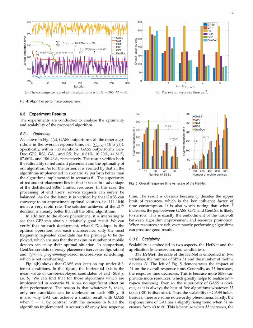
6.3.1 OptimalityAs shown in Fig. 4(a), GASS outperforms all the other algo-rithms in the overall response time, i.e.,

∑i∈N τ(E(s(i))).

Specifically, within 300 iterations, GASS outperforms Gen-Doc, GP2, RS2, GA1, and RS1 by 10.81%, 16.20%, 44.81%,67.66%, and 196.43%, respectively. The result verifies boththe rationality of redundant placement and the optimality ofour algorithm. As for the former, it is verified by that all thealgorithms implemented in scenario #2 perform better thanthe algorithms implemented in scenario #1. The superiorityof redundant placement lies in that it takes full advantageof the distributed SBSs’ limited resources. In this case, theprocessing of end users’ service requests can surely bebalanced. As for the latter, it is verified by that GASS canconverge to an approximate optimal solution, i.e. 111.1040ms at a very rapid rate. The solution achieved at the 21th

iteration is already better than all the other algorithms.In addition to the above phenomena, it is interesting to

see that GP2 can obtain a relatively good result. We canverify that for each deployment, what GP2 adopts is theoptimal operation. For each microservice, only the mostfrequently requested candidate has the privilege to be de-ployed, which ensures that the maximum number of mobiledevices can enjoy their optimal situation. In comparison,GenDoc consists of greedy placement (server configuration)and dynamic programming-based microservice scheduling,which is not overbearing.

Fig. 4(b) shows that GASS can keep on top under dif-ferent conditions. In this figure, the horizontal axis is themean value of can-be-deployed candidates of each SBS j,i.e. bj . We can find that for those algorithms which areimplemented in scenario #1, b has no significant effect ontheir performance. The reason is that whatever bj takes,only one candidate can be deployed on each SBS j. Itis also why GA1 can achieve a similar result with GASSwhen b = 1. By contrast, with the increase in b, all thealgorithms implemented in scenario #2 enjoy less response

10 20 40 80Number of SBSs

0

50

100

150

200

250

300

350

Ove

rall r

espo

nse

time

100 200 400 600 800Number of mobile devices

0

50

100

150

200

250

300

Ove

rall r

espo

nse

time

GASSGP2GA1RS2GenDoc

76.2661<latexit sha1_base64="9v1+lDOR1Wz3hYoVZgHZXaKXs1Q=">AAAB7nicbVBNS8NAEJ34WetX1aOXxSJ4CkmR1mPRi8cK9gPaUDbbbbt0swm7E6GE/ggvHhTx6u/x5r9x2+agrQ8GHu/NMDMvTKQw6Hnfzsbm1vbObmGvuH9weHRcOjltmTjVjDdZLGPdCanhUijeRIGSdxLNaRRK3g4nd3O//cS1EbF6xGnCg4iOlBgKRtFK7VrVrVSrfr9U9lxvAbJO/JyUIUejX/rqDWKWRlwhk9SYru8lGGRUo2CSz4q91PCEsgkd8a6likbcBNni3Bm5tMqADGNtSyFZqL8nMhoZM41C2xlRHJtVby7+53VTHN4EmVBJilyx5aJhKgnGZP47GQjNGcqpJZRpYW8lbEw1ZWgTKtoQ/NWX10mr4vqe6z9cl+u3eRwFOIcLuAIfalCHe2hAExhM4Ble4c1JnBfn3flYtm44+cwZ/IHz+QM27I4q</latexit><latexit sha1_base64="9v1+lDOR1Wz3hYoVZgHZXaKXs1Q=">AAAB7nicbVBNS8NAEJ34WetX1aOXxSJ4CkmR1mPRi8cK9gPaUDbbbbt0swm7E6GE/ggvHhTx6u/x5r9x2+agrQ8GHu/NMDMvTKQw6Hnfzsbm1vbObmGvuH9weHRcOjltmTjVjDdZLGPdCanhUijeRIGSdxLNaRRK3g4nd3O//cS1EbF6xGnCg4iOlBgKRtFK7VrVrVSrfr9U9lxvAbJO/JyUIUejX/rqDWKWRlwhk9SYru8lGGRUo2CSz4q91PCEsgkd8a6likbcBNni3Bm5tMqADGNtSyFZqL8nMhoZM41C2xlRHJtVby7+53VTHN4EmVBJilyx5aJhKgnGZP47GQjNGcqpJZRpYW8lbEw1ZWgTKtoQ/NWX10mr4vqe6z9cl+u3eRwFOIcLuAIfalCHe2hAExhM4Ble4c1JnBfn3flYtm44+cwZ/IHz+QM27I4q</latexit><latexit sha1_base64="9v1+lDOR1Wz3hYoVZgHZXaKXs1Q=">AAAB7nicbVBNS8NAEJ34WetX1aOXxSJ4CkmR1mPRi8cK9gPaUDbbbbt0swm7E6GE/ggvHhTx6u/x5r9x2+agrQ8GHu/NMDMvTKQw6Hnfzsbm1vbObmGvuH9weHRcOjltmTjVjDdZLGPdCanhUijeRIGSdxLNaRRK3g4nd3O//cS1EbF6xGnCg4iOlBgKRtFK7VrVrVSrfr9U9lxvAbJO/JyUIUejX/rqDWKWRlwhk9SYru8lGGRUo2CSz4q91PCEsgkd8a6likbcBNni3Bm5tMqADGNtSyFZqL8nMhoZM41C2xlRHJtVby7+53VTHN4EmVBJilyx5aJhKgnGZP47GQjNGcqpJZRpYW8lbEw1ZWgTKtoQ/NWX10mr4vqe6z9cl+u3eRwFOIcLuAIfalCHe2hAExhM4Ble4c1JnBfn3flYtm44+cwZ/IHz+QM27I4q</latexit><latexit sha1_base64="9v1+lDOR1Wz3hYoVZgHZXaKXs1Q=">AAAB7nicbVBNS8NAEJ34WetX1aOXxSJ4CkmR1mPRi8cK9gPaUDbbbbt0swm7E6GE/ggvHhTx6u/x5r9x2+agrQ8GHu/NMDMvTKQw6Hnfzsbm1vbObmGvuH9weHRcOjltmTjVjDdZLGPdCanhUijeRIGSdxLNaRRK3g4nd3O//cS1EbF6xGnCg4iOlBgKRtFK7VrVrVSrfr9U9lxvAbJO/JyUIUejX/rqDWKWRlwhk9SYru8lGGRUo2CSz4q91PCEsgkd8a6likbcBNni3Bm5tMqADGNtSyFZqL8nMhoZM41C2xlRHJtVby7+53VTHN4EmVBJilyx5aJhKgnGZP47GQjNGcqpJZRpYW8lbEw1ZWgTKtoQ/NWX10mr4vqe6z9cl+u3eRwFOIcLuAIfalCHe2hAExhM4Ble4c1JnBfn3flYtm44+cwZ/IHz+QM27I4q</latexit>

77.2574<latexit sha1_base64="xxR2iMcEkdXsmYj/pjxxnb7EU/A=">AAAB7nicbVBNS8NAEJ31s9avqkcvi0XwFJJSiceiF48V7Ae0oWy2m3bpZhN2N0IJ/RFePCji1d/jzX/jts1BWx8MPN6bYWZemAqujet+o43Nre2d3dJeef/g8Oi4cnLa1kmmKGvRRCSqGxLNBJesZbgRrJsqRuJQsE44uZv7nSemNE/ko5mmLIjJSPKIU2Ks1PF9p3bt1weVquu4C+B14hWkCgWag8pXf5jQLGbSUEG07nluaoKcKMOpYLNyP9MsJXRCRqxnqSQx00G+OHeGL60yxFGibEmDF+rviZzEWk/j0HbGxIz1qjcX//N6mYlugpzLNDNM0uWiKBPYJHj+Ox5yxagRU0sIVdzeiumYKEKNTahsQ/BWX14n7ZrjuY73UK82bos4SnAOF3AFHvjQgHtoQgsoTOAZXuENpegFvaOPZesGKmbO4A/Q5w89AI4u</latexit><latexit sha1_base64="xxR2iMcEkdXsmYj/pjxxnb7EU/A=">AAAB7nicbVBNS8NAEJ31s9avqkcvi0XwFJJSiceiF48V7Ae0oWy2m3bpZhN2N0IJ/RFePCji1d/jzX/jts1BWx8MPN6bYWZemAqujet+o43Nre2d3dJeef/g8Oi4cnLa1kmmKGvRRCSqGxLNBJesZbgRrJsqRuJQsE44uZv7nSemNE/ko5mmLIjJSPKIU2Ks1PF9p3bt1weVquu4C+B14hWkCgWag8pXf5jQLGbSUEG07nluaoKcKMOpYLNyP9MsJXRCRqxnqSQx00G+OHeGL60yxFGibEmDF+rviZzEWk/j0HbGxIz1qjcX//N6mYlugpzLNDNM0uWiKBPYJHj+Ox5yxagRU0sIVdzeiumYKEKNTahsQ/BWX14n7ZrjuY73UK82bos4SnAOF3AFHvjQgHtoQgsoTOAZXuENpegFvaOPZesGKmbO4A/Q5w89AI4u</latexit><latexit sha1_base64="xxR2iMcEkdXsmYj/pjxxnb7EU/A=">AAAB7nicbVBNS8NAEJ31s9avqkcvi0XwFJJSiceiF48V7Ae0oWy2m3bpZhN2N0IJ/RFePCji1d/jzX/jts1BWx8MPN6bYWZemAqujet+o43Nre2d3dJeef/g8Oi4cnLa1kmmKGvRRCSqGxLNBJesZbgRrJsqRuJQsE44uZv7nSemNE/ko5mmLIjJSPKIU2Ks1PF9p3bt1weVquu4C+B14hWkCgWag8pXf5jQLGbSUEG07nluaoKcKMOpYLNyP9MsJXRCRqxnqSQx00G+OHeGL60yxFGibEmDF+rviZzEWk/j0HbGxIz1qjcX//N6mYlugpzLNDNM0uWiKBPYJHj+Ox5yxagRU0sIVdzeiumYKEKNTahsQ/BWX14n7ZrjuY73UK82bos4SnAOF3AFHvjQgHtoQgsoTOAZXuENpegFvaOPZesGKmbO4A/Q5w89AI4u</latexit><latexit sha1_base64="xxR2iMcEkdXsmYj/pjxxnb7EU/A=">AAAB7nicbVBNS8NAEJ31s9avqkcvi0XwFJJSiceiF48V7Ae0oWy2m3bpZhN2N0IJ/RFePCji1d/jzX/jts1BWx8MPN6bYWZemAqujet+o43Nre2d3dJeef/g8Oi4cnLa1kmmKGvRRCSqGxLNBJesZbgRrJsqRuJQsE44uZv7nSemNE/ko5mmLIjJSPKIU2Ks1PF9p3bt1weVquu4C+B14hWkCgWag8pXf5jQLGbSUEG07nluaoKcKMOpYLNyP9MsJXRCRqxnqSQx00G+OHeGL60yxFGibEmDF+rviZzEWk/j0HbGxIz1qjcX//N6mYlugpzLNDNM0uWiKBPYJHj+Ox5yxagRU0sIVdzeiumYKEKNTahsQ/BWX14n7ZrjuY73UK82bos4SnAOF3AFHvjQgHtoQgsoTOAZXuENpegFvaOPZesGKmbO4A/Q5w89AI4u</latexit>

17.30<latexit sha1_base64="FE72KQ8oLzX3+NTYb1+WJJU25nY=">AAAB7HicbVBNS8NAEJ3Ur1q/qh69LBbBU0hUqMeiF48VTFtoQ9lsJ+3SzSbsboRS+hu8eFDEqz/Im//GbZuDVh8MPN6bYWZelAmujed9OaW19Y3NrfJ2ZWd3b/+genjU0mmuGAYsFanqRFSj4BIDw43ATqaQJpHAdjS+nfvtR1Sap/LBTDIMEzqUPOaMGisFft299PrVmud6C5C/xC9IDQo0+9XP3iBleYLSMEG17vpeZsIpVYYzgbNKL9eYUTamQ+xaKmmCOpwujp2RM6sMSJwqW9KQhfpzYkoTrSdJZDsTakZ61ZuL/3nd3MTX4ZTLLDco2XJRnAtiUjL/nAy4QmbExBLKFLe3EjaiijJj86nYEPzVl/+S1oXre65/f1Vr3BRxlOEETuEcfKhDA+6gCQEw4PAEL/DqSOfZeXPel60lp5g5hl9wPr4BP2+NpQ==</latexit><latexit sha1_base64="FE72KQ8oLzX3+NTYb1+WJJU25nY=">AAAB7HicbVBNS8NAEJ3Ur1q/qh69LBbBU0hUqMeiF48VTFtoQ9lsJ+3SzSbsboRS+hu8eFDEqz/Im//GbZuDVh8MPN6bYWZelAmujed9OaW19Y3NrfJ2ZWd3b/+genjU0mmuGAYsFanqRFSj4BIDw43ATqaQJpHAdjS+nfvtR1Sap/LBTDIMEzqUPOaMGisFft299PrVmud6C5C/xC9IDQo0+9XP3iBleYLSMEG17vpeZsIpVYYzgbNKL9eYUTamQ+xaKmmCOpwujp2RM6sMSJwqW9KQhfpzYkoTrSdJZDsTakZ61ZuL/3nd3MTX4ZTLLDco2XJRnAtiUjL/nAy4QmbExBLKFLe3EjaiijJj86nYEPzVl/+S1oXre65/f1Vr3BRxlOEETuEcfKhDA+6gCQEw4PAEL/DqSOfZeXPel60lp5g5hl9wPr4BP2+NpQ==</latexit><latexit sha1_base64="FE72KQ8oLzX3+NTYb1+WJJU25nY=">AAAB7HicbVBNS8NAEJ3Ur1q/qh69LBbBU0hUqMeiF48VTFtoQ9lsJ+3SzSbsboRS+hu8eFDEqz/Im//GbZuDVh8MPN6bYWZelAmujed9OaW19Y3NrfJ2ZWd3b/+genjU0mmuGAYsFanqRFSj4BIDw43ATqaQJpHAdjS+nfvtR1Sap/LBTDIMEzqUPOaMGisFft299PrVmud6C5C/xC9IDQo0+9XP3iBleYLSMEG17vpeZsIpVYYzgbNKL9eYUTamQ+xaKmmCOpwujp2RM6sMSJwqW9KQhfpzYkoTrSdJZDsTakZ61ZuL/3nd3MTX4ZTLLDco2XJRnAtiUjL/nAy4QmbExBLKFLe3EjaiijJj86nYEPzVl/+S1oXre65/f1Vr3BRxlOEETuEcfKhDA+6gCQEw4PAEL/DqSOfZeXPel60lp5g5hl9wPr4BP2+NpQ==</latexit><latexit sha1_base64="FE72KQ8oLzX3+NTYb1+WJJU25nY=">AAAB7HicbVBNS8NAEJ3Ur1q/qh69LBbBU0hUqMeiF48VTFtoQ9lsJ+3SzSbsboRS+hu8eFDEqz/Im//GbZuDVh8MPN6bYWZelAmujed9OaW19Y3NrfJ2ZWd3b/+genjU0mmuGAYsFanqRFSj4BIDw43ATqaQJpHAdjS+nfvtR1Sap/LBTDIMEzqUPOaMGisFft299PrVmud6C5C/xC9IDQo0+9XP3iBleYLSMEG17vpeZsIpVYYzgbNKL9eYUTamQ+xaKmmCOpwujp2RM6sMSJwqW9KQhfpzYkoTrSdJZDsTakZ61ZuL/3nd3MTX4ZTLLDco2XJRnAtiUjL/nAy4QmbExBLKFLe3EjaiijJj86nYEPzVl/+S1oXre65/f1Vr3BRxlOEETuEcfKhDA+6gCQEw4PAEL/DqSOfZeXPel60lp5g5hl9wPr4BP2+NpQ==</latexit>

18.13<latexit sha1_base64="YIObVRy8oQBqyKFwKw6Ss0RXv+0=">AAAB7HicbVBNS8NAEJ3Ur1q/qh69LBbBU8hqwR6LXjxWMG2hDWWz3bRLN5uwuxFK6G/w4kERr/4gb/4bt20O2vpg4PHeDDPzwlRwbTzv2yltbG5t75R3K3v7B4dH1eOTtk4yRZlPE5Gobkg0E1wy33AjWDdVjMShYJ1wcjf3O09MaZ7IRzNNWRCTkeQRp8RYyccNF18PqjXP9RZA6wQXpAYFWoPqV3+Y0Cxm0lBBtO5hLzVBTpThVLBZpZ9plhI6ISPWs1SSmOkgXxw7QxdWGaIoUbakQQv190ROYq2ncWg7Y2LGetWbi/95vcxEjSDnMs0Mk3S5KMoEMgmaf46GXDFqxNQSQhW3tyI6JopQY/Op2BDw6svrpH3lYs/FD/Va87aIowxncA6XgOEGmnAPLfCBAodneIU3RzovzrvzsWwtOcXMKfyB8/kDQniNpw==</latexit><latexit sha1_base64="YIObVRy8oQBqyKFwKw6Ss0RXv+0=">AAAB7HicbVBNS8NAEJ3Ur1q/qh69LBbBU8hqwR6LXjxWMG2hDWWz3bRLN5uwuxFK6G/w4kERr/4gb/4bt20O2vpg4PHeDDPzwlRwbTzv2yltbG5t75R3K3v7B4dH1eOTtk4yRZlPE5Gobkg0E1wy33AjWDdVjMShYJ1wcjf3O09MaZ7IRzNNWRCTkeQRp8RYyccNF18PqjXP9RZA6wQXpAYFWoPqV3+Y0Cxm0lBBtO5hLzVBTpThVLBZpZ9plhI6ISPWs1SSmOkgXxw7QxdWGaIoUbakQQv190ROYq2ncWg7Y2LGetWbi/95vcxEjSDnMs0Mk3S5KMoEMgmaf46GXDFqxNQSQhW3tyI6JopQY/Op2BDw6svrpH3lYs/FD/Va87aIowxncA6XgOEGmnAPLfCBAodneIU3RzovzrvzsWwtOcXMKfyB8/kDQniNpw==</latexit><latexit sha1_base64="YIObVRy8oQBqyKFwKw6Ss0RXv+0=">AAAB7HicbVBNS8NAEJ3Ur1q/qh69LBbBU8hqwR6LXjxWMG2hDWWz3bRLN5uwuxFK6G/w4kERr/4gb/4bt20O2vpg4PHeDDPzwlRwbTzv2yltbG5t75R3K3v7B4dH1eOTtk4yRZlPE5Gobkg0E1wy33AjWDdVjMShYJ1wcjf3O09MaZ7IRzNNWRCTkeQRp8RYyccNF18PqjXP9RZA6wQXpAYFWoPqV3+Y0Cxm0lBBtO5hLzVBTpThVLBZpZ9plhI6ISPWs1SSmOkgXxw7QxdWGaIoUbakQQv190ROYq2ncWg7Y2LGetWbi/95vcxEjSDnMs0Mk3S5KMoEMgmaf46GXDFqxNQSQhW3tyI6JopQY/Op2BDw6svrpH3lYs/FD/Va87aIowxncA6XgOEGmnAPLfCBAodneIU3RzovzrvzsWwtOcXMKfyB8/kDQniNpw==</latexit><latexit sha1_base64="YIObVRy8oQBqyKFwKw6Ss0RXv+0=">AAAB7HicbVBNS8NAEJ3Ur1q/qh69LBbBU8hqwR6LXjxWMG2hDWWz3bRLN5uwuxFK6G/w4kERr/4gb/4bt20O2vpg4PHeDDPzwlRwbTzv2yltbG5t75R3K3v7B4dH1eOTtk4yRZlPE5Gobkg0E1wy33AjWDdVjMShYJ1wcjf3O09MaZ7IRzNNWRCTkeQRp8RYyccNF18PqjXP9RZA6wQXpAYFWoPqV3+Y0Cxm0lBBtO5hLzVBTpThVLBZpZ9plhI6ISPWs1SSmOkgXxw7QxdWGaIoUbakQQv190ROYq2ncWg7Y2LGetWbi/95vcxEjSDnMs0Mk3S5KMoEMgmaf46GXDFqxNQSQhW3tyI6JopQY/Op2BDw6svrpH3lYs/FD/Va87aIowxncA6XgOEGmnAPLfCBAodneIU3RzovzrvzsWwtOcXMKfyB8/kDQniNpw==</latexit>

Fig. 5. Overall response time vs. scale of the HetNet.

time. The result is obvious because bj decides the upperlimit of resources, which is the key influence factor oftime consumption. It is also worth noting that when bincreases, the gap between GASS, GP2, and GenDoc is likelyto narrow. This is exactly the embodiment of the trade-offbetween algorithm improvement and resource promotion.When resources are rich, even poorly performing algorithmscan produce good results.

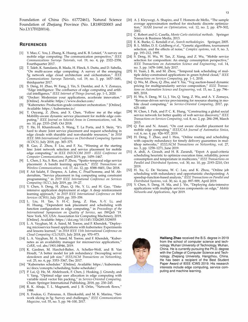
6.3.2 ScalabilityScalability is embodied in two aspects, the HetNet and theapplication (microservices and candidates).

The HetNet: the scale of the HetNet is embodied in twovariables, the number of SBSs M and the number of mobiledevices N . The left of Fig. 5 demonstrates the impact ofM on the overall response time. Generally, as M increases,the response time decreases. This is because more SBSs canprovide more resources, which greatly helps to realize near-request processing. Even so, the superiority of GASS is obvi-ous, as it is always the best of five algorithms whatever Mtakes (RS1 is discarded). Thus, the scalability of GASS holds.Besides, there are some noteworthy phenomena. Firstly, theresponse time of GA1 has a slightly rising trend when M in-creases from 40 to 80. This is because when M increases, the

11

5 10 15 20Number of microservices

0

50

100

150

200

250

300

350

400

Ove

rall

resp

onse

tim

e

GASSGP2GA1RS2GenDoc

Fig. 6. Overall response time vs. number of the microservices.

1 2 3 4 5

Number of finished microservices

0.02

0.04

0.06

0.08

0.1

Ave

rage

Com

plet

ion

time

GASSGP2GenDoc

0 2 4 6 8 10

Number of finished microservices

0

0.05

0.1

0.15

0.2

0.25

Ave

rage

Com

plet

ion

time

GASSGP2GenDoc

0 5 10 15

Number of finished microservices

0

0.1

0.2

0.3

0.4

0.5

Ave

rage

Com

plet

ion

time

GASSGP2GenDoc

0 5 10 15 20

Number of finished microservices

0

0.2

0.4

0.6

Ave

rage

Com

plet

ion

time

GASSGP2GenDoc

Fig. 7. Average response time vs. number of the microservices.

dimension of feasible solution increases, which greatly ex-pands the solution space. Meanwhile, the connected graphof SBSs become sparse, which leads to more hops to transferdata streams. Under this circumstances, 300 iterations mightnot be enough to achieve an optimal enough solution.However, GASS is not effected because the solution space ofGASS is much smaller. The phenomenon verifies the secondadvantage displayed in Subsection 4.4. Secondly, when Mincreases, the gap between GASS, GP2, and GenDoc is likelyto narrow. This phenomenon has been captured in Fig. 4(b).No matter increasing M or b, the resources of SBSs areincreasing, and poorly performing algorithms can producegood results.

The right of Fig. 5 demonstrates the impact of M on theoverall response time. For all the implemented algorithms,the overall response time increases as N increases whilethe solution achieved by GASS is always the best. It isinteresting that the gaps between those benchmark policiesand GASS increase as N increases. It indicates that GASS isrobust to the computation complexity of the fitness function.Thus, the scalability of GASS holds.

The application: the scale of the application is em-bodied in two variables, the number of microservices Q

1 2 3 4 50

50

100

150

200

250

300

Ove

rall

resp

onse

tim

e

GASSGP2GA1RS2GenDoc

Fig. 8. Overall response time vs. C.

and the average number of candidates per microserviceC , 1

Q

∑q∈Q Cq . It can be concluded that GenDoc and

GP2 are competitive while RS1, RS2 and GA1 are obviouslylagging behind. Thus, in the following analysis, we onlycompare GASS with GenDoc and GP2 in terms of theaverage completion time.

Fig. 6 and Fig. 7 demonstrates the impact of the scale ofmicroservices. From Fig. 6 we can find that GASS can keepon top whatever Q is. Correspondingly, Fig. 7 demonstratesthe involution of the average completion time per mobiledevice when Q is 5, 10, 15, and 20, respectively. In allcases, GASS achieves the minimum average completiontime no matter how many microservices have been finished.In our experiments, the maximum E[

∑q∈Q Cq] is 70 while

E[∑j∈M bj ] is 160. Theoretically, if the expected number

of all candidates E[∑q∈Q Cq] does not exceed the expected

number of all the can-be-deployed candidates E[∑j∈M bj ],

GASS can maintain its competitive edge. This is becauseno requests from end users need to be processed by cloud,and the time-consuming backbone can be saved. This ad-vantage is not hold by the benchmark policies. Fig. 8 andFig. 9 demonstrates the impact of the scale of candidates.Similarly, from Fig. 8, we can find that GASS outperformsGP2 and GenDoc in most cases. From Fig. 9 we can find thatGASS always achieves the minimum average completiontime when C is 2, 3, 4, and 5.

Fig. 6 ∼ Fig. 9 verifies that the scalability of GASS holdsin terms of the number of microservices and candidates.

TABLE 3Impact of population size, crossover probability, and mutation

probability.

P∑

i∈N τi Pc∑

i∈N τi Pm∑

i∈N τi

5 114.6762 20% 114.5866 20% 110.4808

10 109.9742 40% 112.2296 40% 105.8360

15 109.6814 60% 116.8252 60% 112.7771

20 113.4527 80% 111.4439 80% 109.2450

25 111.8812 100% 116.1299 100% 112.6478

12

2 4 6 8 10

Number of finished microservices

0

0.05

0.1

0.15

0.2A

vera

ge C

ompl

etio

n tim

eGASSGP2GenDoc

2 4 6 8 10

Number of finished microservices

0

0.05

0.1

0.15

0.2

0.25

Ave

rage

Com

plet

ion

time

GASSGP2GenDoc

2 4 6 8 10

Number of finished microservices

0

0.05

0.1

0.15

0.2

0.25

Ave

rage

Com

plet

ion

time

GASSGP2GenDoc

2 4 6 8 10

Number of finished microservices

0

0.05

0.1

0.15

0.2

0.25

Ave

rage

Com

plet

ion

time

GASSGP2GenDoc

Fig. 9. Average response time vs. C.

Ths superparameters of GASS: Table 3 demonstratesthe overall response time of GASS under different popu-lation size, probability of mutation Pm, and probability ofcrossover Pc, respectively. We can find that their impactis minor on the optimality of GASS. As a result, no moredetailed discussion is launched.

7 RELATED WORKS

Service computing based on traditional cloud data-centershas been extensively studied in the last several years,especially service selection for composition [24] [25] [26],service provision [27], discovery [28], and so on. However,putting everything about services onto the distributed andheterogenous edge is still an area waiting for exploration.Multi-access Edge computing, as a increasingly popularcomputation paradigm, is facing the transition from theoryto practice. The key to the transition is the placement anddeployment of service instances.

In the last two years, service placement at the distributededge has been tentatively explored from the perspective ofQuality of Experience (QoE) of end users or the budgetof ASPs. For example, Ouyang et al. study the problemin a mobility-aware and dynamic way [6]. Their goal isto optimize the long-term time averaged migration costtriggered by user mobility. They develop two efficient heuris-tic schemes based on the Markov approximation and bestresponse update techniques to approach a near-optimalsolution. System stability is also guaranteed by Laypunovoptimization technique. Chen et al. study the problem in aspatio-temporal way, under a limited budget of ASPs [9].They pose the problem as a combinatorial contextual banditlearning problem and utilize Multi-armed Bandit (MAB)theory to learn the optimal placement policy. However, theproposed algorithm is time-consuming and faces the curseof dimensionality. Except for the typical examples listedabove, there also exist works dedicated on joint resourceallocation and load balancing in service placement [7] [8][10] [29]. However, as we have mentioned before, thoseworks only study the to-be-placed services in an atomic way.The correlated and composite property of services is nottaken into consideration. Besides, those works do not tell ushow to apply their algorithms to the service deployment in

a practical system. To address these deficiencies, we navi-gate the service placement and deployment from the viewof production practices. Specifically, we adopt redundantplacement to the correlated microservices, which can beunified managed by Kubernetes.

The idea of redundancy has been studied in parallel-server systems and computing clusters [30] [31] [32]. Thebasic idea of redundancy is dispatching the same job tomultiple servers. The job is considered done as soon as itcompletes service on any one server [15]. Typical job redun-dancy model is the S&X model, where X is the job’s inher-ent size, and S is the server slowdown. It is designed basedon the weakness of the traditional Independent Runtimes(IR) model, where a job’s replicas experience independentruntimes across servers. Unfortunately, although the S&Xmodel indeed captures the practical characteristics of realsystems, it still face great challenges to put it into use inservice deployment at the edge bacause the geographicallydistribution and heterogeneity of edge sites are not consid-ered. To solve the problem, in this paper we redesign theentire model while the idea of redundancy is kept.

This work significantly extends our preliminary work[33]. To improve the practicability, we analyze the responsetime of each mobile device in a more rigorous manner, andimprove it by always finding the nearest available edgesite. We also take the uncertainty of end users’ servicecomposition scheme into consideration. It greatly increasesthe complexity but is of signality. Most important of all, weembedd the idea of redundancy into the problem and designan algorithm with a faster convergence rate.

8 CONCLUSION

In this paper, we study a redundant placement policy forthe deployment of microservice-based applications at thedistributed edge. We first demonstrate the typical HetNetin the near future, and then explore the possibilities of thedeployment of composite microservices with containers andKubernetes. After that, we model the redundant placementas a stochastic optimization problem. For the applicationwith composite and correlated microservices, we design theSAA-based framework SAA-RP and the GASS algorithm todispatch microservice instances into edge sites. By creatingmultiple access to services, our policy boosts a faster re-sponse for mobile devices significantly. SAA-RP not onlytake the uncertainty of microservice composition schemes ofend users, but also the heterogeneity of edge sites into con-sideration. The experimental results based on a real-worlddataset show both the optimality of redundant placementand the efficiency of GASS. In addition, we give guidanceon the implementation of SAA-RP with Kubernetes. In ourfuture work, we will hammer at the implementation of theredundant deployment of complex DAGs with arbitraryshape.

ACKNOWLEDGMENTS

This research was partially supported by the NationalKey Research and Development Program of China (No.2017YFB1400601), Key Research and Development Projectof Zhejiang Province (No. 2017C01015), National Science

13

Foundation of China (No. 61772461), Natural ScienceFoundation of Zhejiang Province (No. LR18F020003 andNo.LY17F020014).

REFERENCES

[1] Y. Mao, C. You, J. Zhang, K. Huang, and K. B. Letaief, “A survey onmobile edge computing: The communication perspective,” IEEECommunications Surveys Tutorials, vol. 19, no. 4, pp. 2322–2358,Fourthquarter 2017.

[2] T. Taleb, K. Samdanis, B. Mada, H. Flinck, S. Dutta, and D. Sabella,“On multi-access edge computing: A survey of the emerging5g network edge cloud architecture and orchestration,” IEEECommunications Surveys Tutorials, vol. 19, no. 3, pp. 1657–1681,thirdquarter 2017.

[3] S. Deng, H. Zhao, W. Fang, J. Yin, S. Dustdar, and A. Y. Zomaya,“Edge intelligence: The confluence of edge computing and artifi-cial intelligence,” IEEE Internet of Things Journal, pp. 1–1, 2020.

[4] “Docker: Modernize your applications, accelerate innovation.”[Online]. Available: https://www.docker.com/

[5] “Kubernetes: Production-grade container orchestration.” [Online].Available: https://kubernetes.io/

[6] T. Ouyang, Z. Zhou, and X. Chen, “Follow me at the edge:Mobility-aware dynamic service placement for mobile edge com-puting,” IEEE Journal on Selected Areas in Communications, vol. 36,no. 10, pp. 2333–2345, Oct 2018.

[7] T. He, H. Khamfroush, S. Wang, T. La Porta, and S. Stein, “It’shard to share: Joint service placement and request scheduling inedge clouds with sharable and non-sharable resources,” in 2018IEEE 38th International Conference on Distributed Computing Systems(ICDCS), July 2018, pp. 365–375.

[8] B. Gao, Z. Zhou, F. Liu, and F. Xu, “Winning at the startingline: Joint network selection and service placement for mobileedge computing,” in IEEE INFOCOM 2019 - IEEE Conference onComputer Communications, April 2019, pp. 1459–1467.

[9] L. Chen, J. Xu, S. Ren, and P. Zhou, “Spatio–temporal edge serviceplacement: A bandit learning approach,” IEEE Transactions onWireless Communications, vol. 17, no. 12, pp. 8388–8401, Dec 2018.

[10] F. Ait Salaht, F. Desprez, A. Lebre, C. Prud’homme, and M. Ab-derrahim, “Service placement in fog computing using constraintprogramming,” in 2019 IEEE International Conference on ServicesComputing (SCC), July 2019, pp. 19–27.

[11] Y. Chen, S. Deng, H. Zhao, Q. He, Y. Li, and H. Gao, “Data-intensive application deployment at edge: A deep reinforcementlearning approach,” in 2019 IEEE International Conference on WebServices (ICWS), July 2019, pp. 355–359.

[12] L. Liu, H. Tan, S. H.-C. Jiang, Z. Han, X.-Y. Li, andH. Huang, “Dependent task placement and scheduling withfunction configuration in edge computing,” in Proceedings of theInternational Symposium on Quality of Service, ser. IWQoS ’19.New York, NY, USA: Association for Computing Machinery, 2019.[Online]. Available: https://doi.org/10.1145/3326285.3329055

[13] L. A. Vayghan, M. A. Saied, M. Toeroe, and F. Khendek, “Deploy-ing microservice based applications with kubernetes: Experimentsand lessons learned,” in 2018 IEEE 11th International Conference onCloud Computing (CLOUD), July 2018, pp. 970–973.

[14] L. A. Vayghan, M. A. Saied, M. Toeroe, and F. Khendek, “Kuber-netes as an availability manager for microservice applications,”CoRR, vol. abs/1901.04946, 2019.

[15] K. Gardner, M. Harchol-Balter, A. Scheller-Wolf, and B. VanHoudt, “A better model for job redundancy: Decoupling serverslowdown and job size,” IEEE/ACM Transactions on Networking,vol. 25, no. 6, pp. 3353–3367, Dec 2017.

[16] “Kubernetes scheduler.” [Online]. Available: https://kubernetes.io/docs/concepts/scheduling/kube-scheduler/

[17] P. Lai, Q. He, M. Abdelrazek, F. Chen, J. Hosking, J. Grundy, andY. Yang, “Optimal edge user allocation in edge computing withvariable sized vector bin packing,” in Service-Oriented Computing.Cham: Springer International Publishing, 2018, pp. 230–245.

[18] R. K. Ahuja, T. L. Magnanti, and J. B. Orlin, “Network flows,”1988.

[19] X. Foukas, G. Patounas, A. Elmokashfi, and M. K. Marina, “Net-work slicing in 5g: Survey and challenges,” IEEE CommunicationsMagazine, vol. 55, no. 5, pp. 94–100, 2017.

[20] A. J. Kleywegt, A. Shapiro, and T. Homem-de Mello, “The sampleaverage approximation method for stochastic discrete optimiza-tion,” SIAM Journal on Optimization, vol. 12, no. 2, pp. 479–502,2002.

[21] C. Robert and G. Casella, Monte Carlo statistical methods. SpringerScience & Business Media, 2013.

[22] E. K. Burke, G. Kendall et al., Search methodologies. Springer, 2005.[23] B. L. Miller, D. E. Goldberg et al., “Genetic algorithms, tournament

selection, and the effects of noise,” Complex systems, vol. 9, no. 3,pp. 193–212, 1995.

[24] S. Deng, H. Wu, W. Tan, Z. Xiang, and Z. Wu, “Mobile serviceselection for composition: An energy consumption perspective,”IEEE Transactions on Automation Science and Engineering, vol. 14,no. 3, pp. 1478–1490, July 2017.

[25] H. Yuan, J. Bi, and M. Zhou, “Temporal task scheduling of mul-tiple delay-constrained applications in green hybrid cloud,” IEEETransactions on Services Computing, pp. 1–1, 2018.

[26] Q. Wu, M. Zhou, Q. Zhu, and Y. Xia, “Vcg auction-based dynamicpricing for multigranularity service composition,” IEEE Transac-tions on Automation Science and Engineering, vol. 15, no. 2, pp. 796–805, 2018.

[27] H. Wu, S. Deng, W. Li, J. Yin, Q. Yang, Z. Wu, and A. Y. Zomaya,“Revenue-driven service provisioning for resource sharing in mo-bile cloud computing,” in Service-Oriented Computing, 2017, pp.625–640.

[28] W. Chen, I. Paik, and P. C. K. Hung, “Constructing a global socialservice network for better quality of web service discovery,” IEEETransactions on Services Computing, vol. 8, no. 2, pp. 284–298, March2015.

[29] Q. Fan and N. Ansari, “On cost aware cloudlet placement formobile edge computing,” IEEE/CAA Journal of Automatica Sinica,vol. 6, no. 4, pp. 926–937, 2019.

[30] H. Deng, T. Zhao, and I. Hou, “Online routing and schedulingwith capacity redundancy for timely delivery guarantees in mul-tihop networks,” IEEE/ACM Transactions on Networking, vol. 27,no. 3, pp. 1258–1271, June 2019.

[31] A. abdi, A. Girault, and H. R. Zarandi, “Erpot: A quad-criteriascheduling heuristic to optimize execution time, reliability, powerconsumption and temperature in multicores,” IEEE Transactions onParallel and Distributed Systems, vol. 30, no. 10, pp. 2193–2210, Oct2019.

[32] H. Xu, G. De Veciana, W. C. Lau, and K. Zhou, “Online jobscheduling with redundancy and opportunistic checkpointing: Aspeedup-function-based analysis,” IEEE Transactions on Parallel andDistributed Systems, vol. 30, no. 4, pp. 897–909, April 2019.

[33] Y. Chen, S. Deng, H. Ma, and J. Yin, “Deploying data-intensiveapplications with multiple services components on edge,” MobileNetworks and Applications, Apr 2019.

Hailiang Zhao received the B.S. degree in 2019from the school of computer science and tech-nology, Wuhan University of Technology, Wuhan,China. He is currently pursuing the Ph.D. degreewith the College of Computer Science and Tech-nology, Zhejiang University, Hangzhou, China.He has been a recipient of the Best StudentPaper Award of IEEE ICWS 2019. His researchinterests include edge computing, service com-puting and machine learning.

14

Shuiguang Deng is currently a full professorat the College of Computer Science and Tech-nology in Zhejiang University, China, where hereceived a BS and PhD degree both in ComputerScience in 2002 and 2007, respectively. He pre-viously worked at the Massachusetts Institute ofTechnology in 2014 and Stanford University in2015 as a visiting scholar. His research interestsinclude Edge Computing, Service Computing,Mobile Computing, and Business Process Man-agement. He serves as the associate editor for

the journal IEEE Access and IET Cyber-Physical Systems: Theory &Applications. Up to now, he has published more than 100 papers injournals and refereed conferences. In 2018, he was granted the RisingStar Award by IEEE TCSVC. He is a fellow of IET and a senior memberof IEEE.

Zijie Liu received the B.S. degree in 2018 fromthe school of computer science and technology,Huazhong University of Science an Technology,Wuhan, China. He is now pursuing the masterdegree with the College of Computer Scienceand Technology, Zhejiang University, Hangzhou,China. His research interests include edge com-puting and software engineering.

Jianwei Yin received the Ph.D. degree in com-puter science from Zhejiang University (ZJU) in2001. He was a Visiting Scholar with the GeorgiaInstitute of Technology. He is currently a FullProfessor with the College of Computer Science,ZJU. Up to now, he has published more than100 papers in top international journals and con-ferences. His current research interests includeservice computing and business process man-agement. He is an Associate Editor of the IEEETransactions on Services Computing.

Schahram Dustdar is a Full Professor of Com-puter Science (Informatics) with a focus on In-ternet Technologies heading the Distributed Sys-tems Group at the TU Wien. He is Chairmanof the Informatics Section of the Academia Eu-ropaea (since December 9, 2016). He is ele-vated to IEEE Fellow (since January 2016). From2004-2010 he was Honorary Professor of In-formation Systems at the Department of Com-puting Science at the University of Groningen(RuG), The Netherlands.

From December 2016 until January 2017 he was a Visiting Professorat the University of Sevilla, Spain and from January until June 2017he was a Visiting Professor at UC Berkeley, USA. He is a memberof the IEEE Conference Activities Committee (CAC) (since 2016), ofthe Section Committee of Informatics of the Academia Europaea (since2015), a member of the Academia Europaea: The Academy of Europe,Informatics Section (since 2013). He is recipient of the ACM Distin-guished Scientist award (2009) and the IBM Faculty Award (2012). He isan Associate Editor of IEEE Transactions on Services Computing, ACMTransactions on the Web, and ACM Transactions on Internet Technologyand on the editorial board of IEEE Internet Computing. He is the Editor-in-Chief of Computing (an SCI-ranked journal of Springer).