1 deepbinarymask: learning a binary mask for video ... · 1 deepbinarymask: learning a binary mask...

1

DeepBinaryMask: Learning a Binary Mask forVideo Compressive Sensing

Michael Iliadis, Member, IEEE, Leonidas Spinoulas, Member, IEEE,and Aggelos K. Katsaggelos, Fellow, IEEE

Abstract—In this paper, we propose a novel encoder-decoder neural network model referred to as DeepBinaryMask for videocompressive sensing. In video compressive sensing one frame is acquired using a set of coded masks (sensing matrix) from which anumber of video frames is reconstructed, equal to the number of coded masks. The proposed framework is an end-to-end model wherethe sensing matrix is trained along with the video reconstruction. The encoder learns the binary elements of the sensing matrix and thedecoder is trained to recover the unknown video sequence. The reconstruction performance is found to improve when using the trainedsensing mask from the network as compared to other mask designs such as random, across a wide variety of compressive sensingreconstruction algorithms. Finally, our analysis and discussion offers insights into understanding the characteristics of the trained maskdesigns that lead to the improved reconstruction quality.

Index Terms—Deep Learning, Compressive Sensing, Mask Optimization, Binary Mask, Video Reconstruction.

F

1 INTRODUCTION

IN signal processing, Compressive Sensing (CS) is a pop-ular problem which has been incorporated in various

applications [1], [2]. In principle, CS theory suggests that asignal can be perfectly reconstructed using a small numberof random incoherent linear projections by finding solutionsto underdetermined linear systems. The underdeterminedlinear system in CS is defined by,

y = Φx, (1)

where Φ is the Mf × Nf measurement or sensing ma-trix with Mf � Nf . We denote the vectorized versionsof the unknown signal and compressive measurements asx : Nf × 1 and y : Mf × 1, respectively. Thus, having moreunknowns than equations, to guarantee a single solution insystem (1) sparsity on the signal is enforced. Many signals,such as natural images, are sparse in well-known bases(e.g., Wavelet). Therefore, most reconstruction approachesemploy a regularization term F (·) which promotes sparsityof the unknown signal x on some chosen transform domain.Thus, the following minimization problem is sought after,

a = argmina

F (a) s.t. y = ΦDa, (2)

where D is a chosen sparse representation transform result-ing in a sparse a, such that x = Da. For example, in thecase F = ||a||0, the problem in Eq. (2) is translated to a `0minimization problem, which can be solved with standardnumerical methods such as Orthogonal Matching Pursuit(OMP) and Basis Pursuit (BP).

Multiple algorithms have been proposed for reconstruct-ing still images using CS by solving the problem in (2). Theproblem of video compressive sensing (VCS) refers to the

• Michael Iliadis, Leonidas Spinoulas and Aggelos K. Katsaggelos arewith the Department of Electrical Engineering and Computer Science,Northwestern University, Evanston, IL 60201, USAE-mail: [email protected], [email protected],[email protected]

HfWf × × tHfWf ×

∗

∫dt=

Captured frame (y)

Measurementmatrix (Φ)

Spatio-Temporalvolume (x)

HfWf × × t

Fig. 1. Temporal compressive sensing measurement model.

recovery of an unknown spatio-temporal volume from thelimited compressive measurements. There are two differentapproaches in VCS, namely spatial and temporal. SpatialVCS architectures perform spatial multiplexing per mea-surement based on the well-known single-pixel-camera [3]and enable video recovery by expediting the capturing pro-cess [4], [5], [6]. In temporal VCS, multiplexing occurs alongthe time dimension. Figure 1 demonstrates this process,where a spatio-temporal signal of size Wf ×Hf × t = Nf ismodulated by t binary random masks during the exposuretime of a single capture and produces a coded frame of sizeWf ×Hf = Mf . The acquisition model in (1) applies to thetemporal VCS case as well. However, the construction of Φis different in this case. In particular, it is sparse and is givenby,

Φ = [diag(φ1), . . . , diag(φt)] : Mf ×Nf , (3)

where each vectorized sampling mask is expressed asφ1, . . . , φt and diag(·) creates a diagonal matrix from itsvector argument. It is noted here that the spatio-temporalvolume is lexicographically ordered into the vector x byconsidering first the spatial and then the temporal dimen-sions.

Performance guarantees for sparse reconstruction meth-ods, i.e., OMP, indicate that matrix Φ must be an incoherentunit norm tight frame [7]. Incoherence is a property that

arX

iv:1

607.

0334

3v2

[cs

.CV

] 1

8 Ju

l 201

6

2

characterizes the degree of similarity between the columnsof Φ (or ΦD). Therefore, the choice of matrix Φ is crucialfor the reconstructed image and video quality irrespectivelyof the choice of F (·). For signals that can be representedsparsely in some basis, various popular matrices in theliterature are known to perform particularly well (e.g.,Gaussian). However, in VCS the design of Φ as part ofthe acquisition hardware (e.g., camera) introduces certainlimitations. For practical implementations, binary randommatrices (e.g., Bernoulli) are better suited while they per-form favorably to Gaussian random matrices [8].

The problem of optimizing the Φ matrix has been ana-lyzed by several researchers [7], [9], [10], [11]. Unfortunately,optimization approaches typically rely on minimizing thecoherence between the sampling matrix Φ and the sparsify-ing basis (ΦD), which mostly applies to spatial compressivesensing where dense matrices are used. Instead, the masksused for temporal VCS systems, as the one described herein,result in a sparse binary matrix with entries across diago-nals, as presented by Eq. (3), and therefore existing resultsare not applicable.

In this work, we optimize the sensing matrix Φ fortemporal VCS and transform it into a form that is moresuitable for reconstruction using deep neural networks. Theproposed neural network architecture, which we refer toas DeepBinaryMask, consists of two components that act asa pair of an encoder and a decoder. The encoder mapsa video block to compressive measurements by learningbinary weights (which correspond to the entries of themeasurement matrix). The decoder maps the measurementsback to a video block utilizing real-valued weights. Bothnetworks are trained jointly. We show that the mask trainedfrom data using neural networks provides significantly im-proved recovery performance as compared to a non-trainedsensing mask.

1.1 Contributions

• Learning binary weights and reconstruction simul-taneously: We propose a novel encoder-decoder neu-ral network for temporal VCS in which the encoderlearns binary weights that form the sensing mask andthe decoder learns to reconstruct the video sequencegiven the encoded measurements.

• Learning a general mask: We show that the recon-struction performance is improved when using theoptimized trained mask over a random one. Perfor-mance improvements are reported not only when thereconstruction method is the neural network decoderbut also when other popular reconstruction methodsare employed (e.g., based on `1 optimization).

• Mask analysis: We present a reconstruction perfor-mance analysis of the trained sensing mask/matrixfor different mask initializations (e.g., initial numberof nonzero elements).

2 MOTIVATION AND RELATED WORK

Recent advances in Deep Neural Networks (DNNs) [12]have demonstrated state-of-the-art performance in severalcomputer vision and image processing tasks, such as

image recognition [13] and object detection [14]. In thissection we briefly discuss previous works in designingoptimal masks for VCS and then we survey recent studiesin image recovery problems using DNNs. Finally, wedescribe advances in DNNs utilizing binary weights, a keyingredient of our proposed method.

Designing optimal masks. Most of the previouslyproposed optimized mask patterns for temporal VCS relyon some heuristic constraints and trial-and-error patterns.A thresholded Gaussian matrix was employed in [15], [16]and [17] as it was assumed that it results in a sensingmatrix that most closely resembles a dense Gaussian matrix.A normalized mask such that the total amount of lightcollected at each pixel is constrained to be constant wasproposed by [18]. It was found in [19] that these normalizedpatterns produce improved reconstruction performance.In [19] a hybrid normalized and Gaussian thresholded maskwas utilized which was found to outperform the masksproposed in [18] and [16].

Differently from these works, our proposed approachdoes not impose any mask constraints but instead generatesmask patterns learnt from the training data. To the bestof our knowledge this is the first study that investigatesthe construction of an optimized binary CS mask throughDNNs.

DNNs for image recovery. The capabilities of deeparchitectures have been investigated in image recoveryproblems such as deconvolution [20], [21], [22],denoising [23], [24], [25], inpainting [26], and super-resolution [27], [28], [29], [30], [31]. Deep architectures havealso been proposed for CS of still images. In [32], stackeddenoising auto-encoders (SDAs) were employed to learn amapping between the CS measurements and image blocks.A similar approach was also utilized in [33] but instead ofSDAs, convolutional neural networks (CNNs) were used.

A closely related study is our previous work in [34]which focuses on learning to map directly temporal VCSmeasurements to video frames using deep fully-connectednetworks when the measurement matrix is fixed. Weshowed that the deep learning framework enables therecovery of video frames from temporal compressivemeasurements in a few seconds at significantly improvedreconstruction quality compared to different, optimizationbased, schemes.

Binary neural networks. Recently, several approacheshave been proposed on the development of neuralnetworks with binary weights [35], [36], [37], [38] forimage recognition applications. The main objective ofsuch an approach is to simplify computations in neuralnetworks, thus making them more efficient while requiringreduced storage. Efficiency is achieved by approximatingthe standard real-valued DNNs with binary weights. InBinaryConnect [36] the authors proposed to binarize theweights for all layers during the forward and backwardpropagations while keeping the real-valued weights duringthe parameter update. The real-valued updates were foundto be necessary for the application of stochastic gradientdescent (SGD). Performance with various classification

3

wp × hp × t

wp × hp × t

wp × hp × t

K hiddenlayers

Inputlayer

Outputlayer

Linear binary mappingof a block to a patch

Block extraction Reshaping into patchInner products along t with binary vectors

Nonlinear mappingof a patch to a block

Reconstruction by averaging overlapping blocks

Measuredframe

Measuredframe

Reconstructedvideo sequence

L1 LK

WkW1 Wo

Inputvideo sequence

Inputvideo sequence

Block divisioninto sub-blocks

Enforcing binary weightsharing for all sub-blocks

Parallel binary layers

Concat.layer

Binarylayer

TRAININGTESTING

Fig. 2. Illustration of the proposed encoder-decoder neural network for video compressive sensing. The bottom part demonstrates the encodernetwork that is responsible for learning the binary mask and outputs CS measurements. The upper part, labeled as “TESTING” illustrates thedecoder network which takes as input CS measurements and outputs a video sequence.

tasks demonstrated that binary neural networks comparefavorably with real-valued weight networks. In [38], theauthors introduced a weight binarization scheme whereboth a binary filter and a scaling factor are estimated.Such scheme was proven more effective compared to theBinaryConnect.

Motivated by the success of DNNs in CS reconstructionand binary DNNs in classification, we investigate in thispaper the problem of learning an optimized binary sensingmatrix using DNNs for temporal VCS.

The work presented in this paper is different from thestudies in image recovery using DNNs and from the binaryneural networks. First, this work is different from our workin [34] since our focus is on learning an optimized sensingmask along with the video reconstruction. In [34] the scopewas to recover video frames directly from the temporalmeasurements (e.g., the mask is pre-defined). Furthermore,our objective in this paper is to learn binary masks that willencode video frames on VCS cameras for video reconstruc-tion which is different from that in binary neural networkstudies, which is efficiency for image recognition problems.

3 DEEPBINARYMASK

In this work, we propose a novel neural network architec-ture that learns to encode a three dimensional (3D) videoblock to compressive two-dimensional (2D) measurementsby learning the binary weights of Φ and to decode the mea-surements back to a video block, as illustrated in Figure 2.Let us now describe in detail the encoder and decoder.

3.1 EncoderIn order for our learning approach to be practical, recon-struction has to be performed on 3D video blocks [33],[34]. Thus, each video block must be sampled with a block-based measurement matrix which should be the same for allblocks. Furthermore, such a measurement matrix should berealizable in hardware. We follow the pattern in [34] and weconsider a Φ which consists of repeated identical buildingblocks of size wp×hp× t = Np corresponding to the matrixΦp of size Mp × Np, where Mp = wp × hp. In other wordsΦp has the structure shown in Eq. (3), in which Mf andNf have been respectively replaced by Mp and Np. Animplementation of such a matrix on existing systems em-ploying Digital Micromirror Devices (DMDs), Spatial LightModulators (SLMs) or Liquid Crystal on Silicon (LCoS) [5],

4

[6], [15], [17], [18] can be easily performed. At the same time,a repeated mask can be printed and shifted appropriatelyto produce the same effect in systems utilizing translatingmasks [16], [19].

Let us consider a set of N training 3D video blocks, eachof size wp × hp × t. They are lexicographically ordered byconsidering first the spatial and then the temporal dimen-sions to form vectors xi, each of size Np × 1. The encoderis defined as the mapping g(·) that transforms each xi toa measurement yi of size Mp × 1, which represents thelexicographically ordered wp × hp image patch, followedby a non-linearity given as,

yi = g(xi; θe) = σe(Φpxi), (4)

where θe = {Φp} is the parameter set and function σe(·) rep-resents the non-linearity. We use the subscript “e” to denotequantities pertaining to the encoder, in order to distinguishthem from the decoder quantities to be introduced later.

The formulation in (4) would have been straightfor-ward to handle if matrix Φp were dense and consisting ofreal-values. However, as mentioned earlier, in the case oftemporal VCS, matrix Φ is binary (due to implementationconsiderations) and sparse following the structure definedin (3). For ease of presentation let us now also define amatrix B of size t×Mp containing the binary weights as,

B =[b1, . . .bMp

]=

b1,1 . . . b1,Mp

.... . .

...bt,1 . . . bt,Mp

. (5)

It is related to the measurement matrix Φp as,

Φp =

b1,1 0 0 bt,1 0 0

0. . . 0 · · · 0

. . . 00 0 b1,Mp

0 0 bt,Mp

. (6)

In order to realize such a structure in a neural network andbe able to train it we transform the encoder into a networkthat involves the following steps:

1) The first step consists of Mp binary parallel layers.To describe this step we need to introduce a newcolumn (t × 1) vector xi,j , which consists of all thetemporal elements at a given spatial location j, thatis,

xi,j =

xi(j)xi(Mp + j)xi(2Mp + j)

...

xi

((t− 1)Mp + j

)

, (7)

where xi(j) denotes the j-th element of vector xi.Then in parallel the following inner products arecomputed,

e(xi,j) = bTj xi,j , for j = 1, ...,Mp. (8)

2) The second step consists of a concatenation layerwhich concatenates the outputs of the parallel layersin order to construct a single measurement vectorthat is,

yi = g(xi; θe) = concat(e(xi,1), . . . , e(xi,Mp

)),

(9)

Full measurement matrix (Φ)

Building su

b-block

Repeat in bothdirections

ws × hs × t

Fig. 3. Construction of the full measurement matrix by repeating a threedimensional random binary array (building sub-block) in the horizontaland vertical directions.

with a parameter set θe = {b1, . . . ,bMp}, as defined

by Eqs. (5) and (6). Note, that a non-linearity suchas the rectified linear unit (ReLU) [39] defined as,σ(z) = max(0, z), is implicitly applied here after theconcatenation since the output is always positive.This is due to the fact that the weights are binarywith values 0 and 1 and the video inputs have non-negative values.

The above two steps follow the model presented in Figure 1but translated to a neural network, where the set θe consistsof the elements of the trained projection matrix. The twosteps of the encoder are illustrated at the bottom part ofFigure 2. Note that the figure refers to the encoding ofoverlapping blocks, as we describe next.

Overlapping blocks and weight sharing. The t × Mp

binary weight matrix B we have considered so farcorresponds to non-overlapping video blocks. In order torealize overlapping blocks which usually aid in improvingreconstruction quality we can utilize repeating blocks ofdimensions wp

2 ×hp

2 × t, which we call sub-blocks as shownin Figure 2. Thus, for the final trained matrix Φp eachwp

2 ×hp

2 × t sub-block is the same allowing reconstructionof overlapping blocks of size wp × hp × t with spatialoverlap of wp

2 ×hp

2 = ws × hs, as presented in Figure 3. Insuch a case the parameter set θe is also different. Instead oflearning Mp binary weight vectors we learn Mp/4, whereeach weight vector is shared four times for each of thecorresponding pixel positions of the input. For example, inthe case when wp × hp = 8 × 8 there will be four identical4 × 4 × t sub-block projection matrices. Notice in Figure 2that the values of the input block at the corresponding pixellocations at each of the sub-blocks are multiplied by thesame binary vector. Thus, for this example, we only need toestimate 16 binary weight vectors and each one is sharedby four different inputs. For instance, in order to calculatee(xi,1), e(xi,5), e(xi,33), e(xi,37) the weight vector b1 isused.

Binary weights. Let us now proceed to describe how toestimate the binary weights. We follow the BinaryConnectmethod [36] to constrain the weights of the encoder to beequal to either 0 or 1 during propagation. The binarizationscheme to transform the real-valued weights to binaryvalues is based on the sign function, that is,

5

bb =

{1 if br ≥ 0,0 otherwise,

(10)

where bb and br are the binarized and real-valued weightsof B, respectively. Following the training process in [36] webinarize the weights of the encoder only during the forwardand backward propagations. The update of the parameterset θe is performed using the real-valued weights. Asexplained in [36], keeping the real-valued weights duringthe updates is necessary for training the networks usingSGD. In addition, we enforced the real-valued weights tolie within the [−1, 1] interval at each training iteration. Theweight clipping was chosen since otherwise the weightsmay become infinitely large having no impact duringbinarization.

Weight initialization. The network weight initializationof the encoder corresponds in our case to the maskinitialization. Typically, in VCS the mask is generatedrandomly. Similarly here, we start with a randomlygenerated mask by a Bernoulli distribution. However,since real-valued weights are also required by the networkto perform their updates we consider the followinginitialization scheme,

bb ∼ Bern (p) ,

br =

∼ Unif

(0, 1/√t)

if bb = 1,

∼ Unif(−1/√t, 0)

otherwise,

(11)

where Bern(·) and Unif(·) denote the Bernoulli and Uni-form distributions, respectively, p is the probability of theweight to be initialized with 1 and notation (·, ·) refersto the lower and upper bounds for the values of the dis-tribution. The bounds of the Uniform distribution followthe scheme introduced in [40]. The initialization schemeproposed above allows us to fully understand the benefits oflearning as compared to non-learning the mask along withreconstructing the video. This is due to the fact that in thecase of choosing the non-learning mode we keep the initialbb weights, drawn from the Bernoulli distribution, fixed.

3.2 Decoder

The resulting hidden measurement yi produced by theencoder is then mapped back to a reconstructed Np × 1vector through the decoder f(yi; θ), which when unstackedresults in the wp × hp × t dimensional video block, asillustrated in the upper part of Figure 2. Thus, the decoderof the proposed method is another network which is trainedto reconstruct the video output sequence given yi. We con-sider a Multi-Layer Perceptron (MLP) architecture to learna nonlinear function f(·) that maps a measured frame patchyi via several hidden layers to a video block xi as in [34].

The output of the kth hidden layer Lk, k = 1, . . . ,K isdefined as,

hk(yi) = σd(Wkhk−1(yi) + ck), with h0(yi) = yi, (12)

where Wk is the output weight matrix, and ck ∈ RNp thebias vector. W1 ∈ RNp×Mp connects yi, the output of theencoder, to the first hidden layer of the decoder, while forthe remaining hidden layers, {W2, . . . ,WK} ∈ RNp×Np .

The last hidden layer is connected to the output layer viaco ∈ RNp and Wo ∈ RNp×Np without nonlinearity. The non-linear function σd(·) is the ReLU and the weights of eachlayer are initialized to random values uniformly distributedin (−1/

√Np, 1/

√Np) [40].

There are several reasons why the MLP architecture forthe decoder is a reasonable choice for the temporal videocompressive sensing problem which have been explainedin [34]. Since our focus in this work is to primarily investi-gate and compare the performance of the trained versus thenon-trained sensing matrix we adopt the decoder designin [34].

3.3 Training the encoder-decoder networkThe two components of the proposed MLP encoder-decoder are jointly trained by learning all the weightsand biases of the model. Using spatial overlap wp

2 ×hp

2 the set of all parameters is denoted by θ ={b1, . . .bMp/4;W1, . . .WK ;Wo; c1, . . . , cK ; co

}and is up-

dated by the backpropagation algorithm [41] minimizingthe quadratic error between the set of the encoded mappedmeasurements f(yi; θ) and the corresponding video blocksxi. The loss function is the Mean Squared Error (MSE) whichis given by,

L(θ) =1

N

N∑

i=1

‖f(yi; θ)− xi‖22. (13)

The MSE was used in this work since our goal is to optimizethe Peak Signal to Noise Ratio (PSNR) which is directlyrelated to the MSE.

Training procedure. The overall training procedurecan be summarized by the following steps:

1) Forward propagation is performed by usingweightsB after binarization in the encoder and real-valued weights W in the decoder.

2) Then, backpropagation is performed to compute thegradients with respect to layer’s activation knowingB and W .

3) Parameter updates are computed using the real-valued weights for both encoder and decoder.

Note that one other difference between our workand [36] is that our encoder-decoder neural network doesnot utilize binary weights in all layers; instead it utilizesbinary weights at the encoder and standard real-valuedweights at the decoder.

Implementation details. Our encoder-decoder neuralnetwork is trained for 480 epochs using a mini-batch sizeof 200. We used SGD with a momentum set equal to 0.9.We further used `2 norm gradient clipping to keep thegradients in a certain range. Gradient clipping is a widelyused technique in recurrent neural networks to avoidexploding gradients [42]. The threshold of gradient clippingwas set equal to 0.1.

One hyper-parameter that was found to affect the per-formance in our approach is the learning rate. Based onexperimentation we chose a starting learning rate for theencoder that was 10 times larger than that for the decoder.

6

This was found to be important as we wanted the weights ofthe encoder to have their sign changed during the trainingiterations. In addition, the learning rate was divided by 2 atevery 10 epochs in the encoder and by 10 after 400 epochsin the decoder.

All hyper-parameters were selected after cross-validation using a validation test set.

Test inference. Once the encoder-decoder neural networkis trained we use the trained sensing matrix B → Φ tocalculate the compressive measurements y. Then, given ywe can use any VCS algorithm (in addition to the decodernetwork) to reconstruct the video blocks.

4 EXPERIMENTAL RESULTS

In this section we present quantitative and qualitative recon-struction results to demonstrate the effectiveness of the pro-posed projection mask in temporal VCS. The performance ofour trained masks is investigated using various reconstruc-tion algorithms and initial mask parameters. Our analysisoffers insights into understanding how the different initialparameters of the mask affect reconstruction performance.The metrics used for reconstruction evaluation were thePSNR and SSIM (Structural SIMilarity).

4.1 Training Data Collection and Test set

In order to train our encoder-decoder architecture we col-lected a diverse set of training samples using 400 high-definition videos from Youtube, depicting natural scenes.The video sequences contain more than 105 frames whichwere converted to grayscale. We randomly extracted 1 mil-lion video blocks of size wp × hp × t to train our encoder-decoder neural network while keeping the amount of blocksextracted per video proportional to its duration.

Our test set consists of 14 video sequences that wereused in [18] which are provided by the authors. We alsoincluded in the test set the “Basketball” video sequence usedin [43]. All test video sequences are unrelated to the trainingset.

4.2 Mask Patterns and Decoding Layers

Our experimental investigation is motivated by the follow-ing two questions: 1) “How does performance of trained andnon-trained masks compare using different reconstructionalgorithms?” and 2) “Does the training procedure result ina unique sensing matrix Φ irrespectively of the initializationparameters?”

In order to answer these two questions we simulatednoiseless compressive video measurements by realizingfour different wp

2 ×hp

2 × t mask patterns. We denote by“RandomMask-p” the mask that is initialized with Bern (p),as in Eq. (11), and is not learnt (that is, the elements ofthe encoder are fixed). We also denote by “DeepMask-p”the learnt mask trained by our proposed encoder-decodernetwork described in section 3 and which is initialized byBern (p) as in Eq (11). Thus, we consider the following fourmask patterns:

• RandomMask-20 and DeepMask-20, with p = 20%.

• RandomMask-40 and DeepMask-40, with p = 40%.• RandomMask-60 and DeepMask-60, with p = 60%.• RandomMask-80 and DeepMask-80, with p = 80%.

For the remainder of this paper, we describe the selectionof block sizes ofwp×hp×t = 8×8×16, such thatNp = 1024and Mp = 64. Therefore, the compression ratio is 1/16. Inaddition, for each of the eight Φ mask types above, eachwp

2 ×hp

2 × t = 4 × 4 × 16 block is the same allowingreconstruction for overlapping blocks of size 8×8×16 withspatial overlap of 4 × 4. Note that the same random seedwas utilized for all patterns.

Further, we used K = 4 hidden layers for the decoderarchitecture of Figure 2. We found out experimentally thatfor the number of training data used (1 million) 4 layersprovided the best performance. A similar observation wasreported in [34] where the addition of extra layers forthis number of training data did not lead to performanceimprovement.

In the following section we present the reconstructionalgorithms used to test the eight mask types.

4.3 Reconstruction AlgorithmsSince our main goal is to compare the performance betweena trained sensing mask over a non-trained one in an imple-mentation agnostic to mask patterns, we tested a number ofdifferent reconstruction algorithms. Candidate reconstruc-tion algorithms were selected for their utility in solving theunderdetermined system in the VCS setting. We evaluatedthe following optimization algorithms as potential solvers:

1) DICT-L1: In (1), we have assumed that data arenoise-free. However, real data are typically noisyand dealing with small dense noise is required. Inorder to deal with such noise we transform the prob-lem in (2) into the LASSO (Least-Absolute Shrinkageand Selection Operator) problem for F = λ||a||1given as,

a = argmina‖y − ΦDa‖22 + λ||a||1, (14)

where λ > 0 is the regularization parameter whosevalue is related to the noise tolerance. For this prob-lem we chose to use an overcomplete dictionaryD as a sparsifying basis. The dictionary consists of20, 000 atoms trained on a subset of 200, 000 videoblocks from our training database and reconstruc-tion is performed block-wise on overlapping sets of7×7 patches of pixels. For the optimization problemin (14), λ was set equal to 0.005.

2) TV-MIN: A popular CS reconstruction method uti-lizes for F (·) the total variation (TV) norm definedas,

TV (z) =∑

i,j,n

((z(i+ 1, j, n)− z(i, j, n)

)2

+(z(i, j + 1, n)− z(i, j, n)

)2)1/2

,

(15)where z is the stacked version of the 3D arrayz(i, j, n), where (i, j, n) are respectively the two

7

Ave

rage

PSN

RInitial binary mask (RandomMask) Optimized binary mask (DeepMask)

24

34

26

28

30

32

Initial percentage of 1’s on mask: 20%




FC4-1M

DICT-L1

TV-MIN

GMM-4

GMM-1

FC4-1M

DICT-L1

TV-MIN

GMM-4

GMM-1

FC4-1M

DICT-L1

TV-MIN

GMM-4

GMM-1

FC4-1M

DICT-L1

TV-MIN

GMM-4

GMM-1.70

.90

.74

.78

.82

.86

Ave

rage

SSI

M

Reconstruction algorithm Reconstruction algorithm Reconstruction algorithm Reconstruction algorithm

Fig. 4. Average PSNR and SSIM over all test video sequences for several reconstruction methods using the RandomMasks and DeepMasks. Thetest set consists of 14 videos sequences and the reported PSNR and SSIM corresponds to the average values for the reconstruction of the first 32frames of each sequence. The PSNR metric is measured in dB while the SSIM is unitless.

spatial and one temporal coordinates. Thus, the TVminimization problem is given as,

x = argminx‖y − Φx‖22 + λTV (x). (16)

In order to solve (16) we used the two-step itera-tive shrinkage/thresholding (TwIST) algorithm [45]with λ = 0.01.

3) GMM-TP: Another reconstruction algorithm weconsidered in our experiments is a Gaussian mix-ture model (GMM)-based algorithm [44] learnedfrom Training Patches (TP) referred as GMM-TP. Wefollowed the settings proposed by the authors andused our training data (randomly selecting 20, 000samples) to train the underlying GMM parameters.In our experiments we refer to this method byGMM-4 and GMM-1 to denote reconstruction ofoverlapping blocks with spatial overlap of 4×4 and1× 1 pixels, respectively.

4) FC4-1M: Finally, another reconstruction method weconsidered is the decoder neural network intro-duced in subsection 3.2. The decoder is a K = 4MLP trained on 1 million samples similarly to [34].In this case, a collection of overlapping patches ofsize 8 × 8 is extracted by each coded measurementof sizeWf×Hf and subsequently reconstructed intovideo blocks of size 8 × 8 × 16. Overlapping areasof the recovered video blocks are then averaged

to obtain the final video reconstruction results asshown in the upper part of Figure 2. The step ofthe overlapping patches was set to 4 × 4 due tothe special construction of the utilized measurementmatrix, as discussed in subsection 3.1.

For each algorithm, λ values were determined basedon the best performance among different settings. All codeimplementations are publicly available provided by theauthors while the deep network architectures were imple-mented in Torch7 [46], a Lua library that allowed us todevelop an optimized GPU code.

4.4 Reconstruction Results

For each reconstruction algorithm described above, wetested the eight mask types presented in subsection 4.2.

Quantitative and qualitative results. Figure 4 showsaverage reconstruction quality for each mask and algorithmcombination, using the PSNR and SSIM metrics. Thepresented metrics refer to average performance for thereconstruction of the first 32 frames of each test videosequence, using 2 consecutive captured coded framesfor each of the eight masks for every algorithm. First,we note that the DeepMasks perform consistently bettercompared to the RandomMasks across all reconstructionalgorithms and initial percentage of nonzeros. In particular,

8

FC4-

1M

33

29

30

31

32

5 10 15 20 25 300

PSN

R31

25

27

29

33

29

30

31

32

24

26

28

30

5 10 15 20 25 300 5 10 15 20 25 300 5 10 15 20 25 300

DIC

T-L1

31

26272829

5 10 15 20 25 300

PSN

R

Frame number

Horse sequence Porsche sequence

Frame number

28

22

24

26

31

27

28

29

30

21

23

25

27

29

5 10 15 20 25 300 5 10 15 20 25 300 5 10 15 20 25 300

GM

M-1

31

28

30

29

5 10 15 20 25 300

PSN

R

29

23

25

27

32

28

29

30

31

22

24

26

28

5 10 15 20 25 300 5 10 15 20 25 300 5 10 15 20 25 300

Frame number Frame number

Horse sequence Porsche sequence

Initial percentage of 1’s on mask: 20% Initial percentage of 1’s on mask: 40%

30

Initial binary mask (RandomMask) Optimized binary mask (DeepMask)

Fig. 5. PSNR (in dB) comparison for the first 32 frames of 2 video sequences among the proposed method FC4-1M and the previous methodsGMM-1 [44] and DICT-L1 [18]. Notice that the vertical scale changes among the various plots.

we observe an improvement around 1-2 dB, in terms ofPSNR between the trained and non-trained masks acrossall initial percentages and algorithms. Furthermore, weobserve that the decoder FC4-1M demonstrates the highestPSNR and SSIM values among all algorithms.

Figure 5 compares the PSNR for each of the 32 framesof 2 video sequences (“Horse” and “Porsche” sequences)using our FC4-1M algorithm and the previous methodsGMM-1 [44] and DICT-L1 [18] between the RandomMasksand DeepMasks. The varying PSNR performance across theframes of a 16 frame block is consistent for all algorithmsand is reminiscent of the reconstruction tendency observedin other video CS papers in the literature [16], [19], [43], [44].Please notice that the scale on the vertical axes of the plotvaries.

Finally, Figure 6 compares the reconstruction qualitybetween the optimized and non-optimized masks for asingle frame from the 2 video sequences under differentalgorithms and different mask initializations. It is clear thatreconstruction quality improves when using the optimizedmasks, especially for the case when the initial percentageof nonzeros is p = 60. At the same time, the proposedend-to-end optimization using the deep network (FC4-1M)provides the highest visual quality among the candidatecompared algorithms.

−1 −0.5 0 0.5 10

20

40

60

80

100

Weight value

Freq

uenc

y

Fig. 7. Histogram of the real-valued weights produced by the en-coder neural network for DeepMask-40. We report similar observationswith [36] as we found out that most of the weights have the tendencyto become deterministic (−1 and 1) and reduce the training error whilesome stay around zero.

4.5 Training analysis

We start our analysis by examining the real-valued weighthistogram of the encoder (DeepMask-40) upon convergencein Figure 7. First, we observe that negative values aremore frequent than positive ones, which suggests that zeroelements of the mask (after binarization) are more importantthan the nonzero ones. More importantly, we observe that

9

Horse Video Sequence Porsche Video SequenceFC

4-1M

Ori

gina

l Fra

me

Initial binary mask Optimized binary mask Initial binary mask Optimized binary mask

PSNR = 31.17, SSIM = 0.8351 PSNR = 29.05, SSIM = 0.9632PSNR = 31.98, SSIM = 0.8582 PSNR = 29.64, SSIM = 0.9686


GM

M-1

DIC

T-L1





p =

40

p =

60

p =

40

p =

60

p =

40

p =

60

Fig. 6. Qualitative reconstruction performance. The figure shows reconstruction of a single frame for 2 test video sequences when using differentreconstruction algorithms and different mask initializations. The PSNR metric is measured in dB while the SSIM is unitless.

a number of weights are around zero, hesitating betweenbecoming negative or positive, a phenomenon that was also

reported in [36].

Average test MSE per epoch calculated on a validation

10

0 100 200 300 400 500−3.8

−3.6

−3.4

−3.2

−3

−2.8

−2.6

−2.4

Epoch

Ave

rage

test

ing

MSE

(log

10) DeepMask (p = 40)

RandomMask (p = 40)

Fig. 8. Test error curves between the RandomMask-40 decoder andDeepMask-40 encoder-decoder calculated on a validation test set. Thelatter provided lower test error upon convergence as is optimized end-to-end.

0 100 200 300 400 500Epoch

0

10

20

30

40

50

60

70

Bina

ry w

eigh

t cha

nges

Fig. 9. Number of binary weight changes per epoch of DeepMask-40encoder-decoder. A large number of weights change in the first fewepochs; this number decreases and finally becomes zero in the last fewepochs.

test set for DeepMask-40 and RandomMask-40 is shownin Figure 8. It is shown that the test error curve of theRandomMask-40 is smooth while the DeepMask-40 is noisy.This is due to the fact that many binary weights switchbetween 1 and 0 frequently, especially during the firstepochs of training when the learning rate has high values,thus constantly changing the way the VCS measurementsare performed. Furthermore, even at the later stages oftraining, many real-valued elements of the encoder remainaround zero, as observed in Figure 7. Therefore, during thebinarization process some of the encoder’s binary weightschange from zero to one and vice versa even with verysmall learning rates. However, as the encoder’s learningrate becomes really small the curve becomes smooth. Abetter optimized learning rate decay schedule of the encoderwould have probably provided a smoother curve and per-haps a higher performance. We leave this as a task for futurework as further investigation into this may be needed.Finally, as showed in the reconstruction results, DeepMaskperforms consistently better than RandomMask which alsoexplains the lower test MSE produced by the former during

Epoch0 100 200 300 400 500

20

30

40

50

60

70

80

90

Perc

enta

ge o

f non

zero

wei

ghts

DeepMask (p = 60)

DeepMask (p = 20)DeepMask (p = 40)

DeepMask (p = 80)

Fig. 10. Percentage of nonzero binary values for DeepMasks. Irrespec-tively to the initial nonzero percentage, DeepMasks converge to a pointaround 40% nonzeros.

training.Lastly, in Figure 9 we show the number of binary weights

that change from zero to one and vice versa per epoch. Weobserve that a large number of weights change in the firstfew epochs and this number decreases as the number ofepochs increases.

5 DISCUSSION

Having obtained better reconstruction performance usingthe DeepMasks across a wide range of reconstructionalgorithms our next step is to analyze the masks producedby the networks and highlight a few crucial points. We startour analysis by posing the following question.

Does DeepMask produce a unique sensing matrixΦ? To answer this question we examine the differencesbetween the produced DeepMasks with respect to theirpercentage of nonzero elements and to their support.

First, in Figure 10 we show the percentage of nonzerobinary weights per epoch for the different DeepMasks.This figure allows us to examine uniqueness with respectto the percentage of nonzero elements produced by eachDeepMask. We observe that the masks with p equal 40, 60and 80 converge to a percentage around 40%. The p = 20%mask though, converges to a bit lower percentage (around38% nonzero binary elements).

Next, Figure 11 demonstrates the four mask patternsproduced in this work. The first row illustrates the Random-Masks and the second row presents the four DeepMasksproduced by the proposed encoder-decoder neural network.All 4 × 4 × 16 masks are reshaped into a 16 × 16 matrixfor better visualization by lexicography ordering each 4× 4mask at a given time instance into a 16 × 1 vector, whichbecomes a column of the 16 × 16 matrix. That is, thevertical direction denotes pixel location while the horizontaldirection denotes time. From the visualization we deducethat although the masks generated by the network convergeto the same nonzero percentage (as shown in Figure 10),their support is different. The fact that the optimized maskscontain a very similar percentage of nonzeros while produc-ing improved reconstruction quality with various different

11

50

40

30

20

10

0

60

50

40

30

20

10

0

60

1 2 3 4 5 6 7 8 9 10 11 12 13 14 1 2 3 4 5 6 7 8 9 10 11 12 13 14

Ave

rage

PSN

R us

ing

FC4-

1MA

vera

ge P

SNR

usin

g FC

4-1M

Video sequence number Video sequence number

DeepMask (Seed 1) DeepMask (Seed 2)



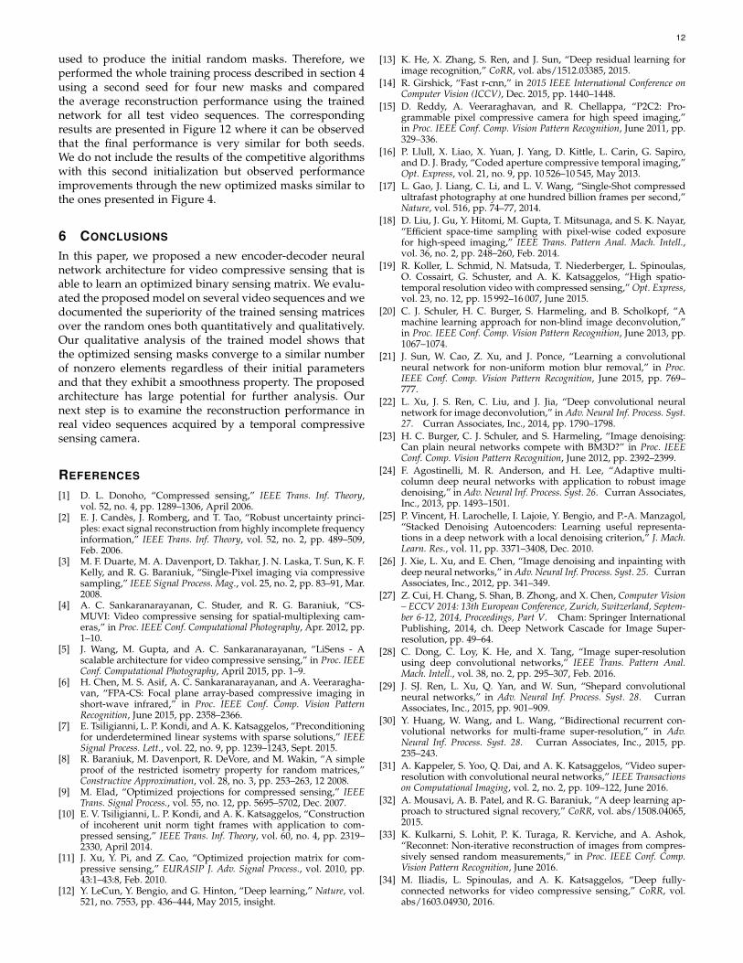
Fig. 12. Comparison of the reconstruction performance of the proposed encoder-decoder architecture when using the optimized masks trainedafter initialization with two different seeds. Average PSNR for the reconstruction of the first 32 frames of each one of the 14 test video sequences ispresented and the values are found to be very similar regardless of the starting binary values of the measurement matrix.

(a) RM-20 (b) RM-40 (c) RM-60 (d) RM-80

(h) DM-80(g) DM-60(f) DM-40(e) DM-20

Spat

ial d

imen

sion

Time dimension

Fig. 11. The eight mask patterns produced in this work of size 16 × 16.The initial RandomMasks (RM) are presented on the top row while onthe bottom row we present the optimized DeepMasks (DM).

reconstruction algorithms implies that such percentage isthe most appropriate one for the task at hand. Similarobservations about the ideal percentage of nonzeros forVCS measurement matrices have been made in [19], albeit

deduced through heuristic experimentation.Finally, from the visualization we deduct two important

findings:

• First, it is apparent that regardless of the initialrealization (shown in RandomMasks), the trainedDeepMasks produce a similar number of nonzeroelements which confirms our findings discussed ear-lier.

• Second, an important observation from Figure 11 isthat DeepMasks are smoother over time than the Ran-domMasks. In other words in many rows the binaryweights seem to be sequential (or more structured)forming runs of 1s and 0s. Again, such finding washeuristically observed in [19] and some studies citedtherein, further strengthening our findings which arehere obtained through a machine learning approach.

To summarize, our observations above suggest that anoptimized mask design Φ for temporal VCS incorporatesthe following two characteristics: 1) smoothness as explainedabove and 2) percentage of nonzero elements around 40%.

Finally, we wanted to confirm that the results presentedherein are not due to a specific selection of the random seed,

12

used to produce the initial random masks. Therefore, weperformed the whole training process described in section 4using a second seed for four new masks and comparedthe average reconstruction performance using the trainednetwork for all test video sequences. The correspondingresults are presented in Figure 12 where it can be observedthat the final performance is very similar for both seeds.We do not include the results of the competitive algorithmswith this second initialization but observed performanceimprovements through the new optimized masks similar tothe ones presented in Figure 4.

6 CONCLUSIONS

In this paper, we proposed a new encoder-decoder neuralnetwork architecture for video compressive sensing that isable to learn an optimized binary sensing matrix. We evalu-ated the proposed model on several video sequences and wedocumented the superiority of the trained sensing matricesover the random ones both quantitatively and qualitatively.Our qualitative analysis of the trained model shows thatthe optimized sensing masks converge to a similar numberof nonzero elements regardless of their initial parametersand that they exhibit a smoothness property. The proposedarchitecture has large potential for further analysis. Ournext step is to examine the reconstruction performance inreal video sequences acquired by a temporal compressivesensing camera.

REFERENCES

[1] D. L. Donoho, “Compressed sensing,” IEEE Trans. Inf. Theory,vol. 52, no. 4, pp. 1289–1306, April 2006.

[2] E. J. Candes, J. Romberg, and T. Tao, “Robust uncertainty princi-ples: exact signal reconstruction from highly incomplete frequencyinformation,” IEEE Trans. Inf. Theory, vol. 52, no. 2, pp. 489–509,Feb. 2006.

[3] M. F. Duarte, M. A. Davenport, D. Takhar, J. N. Laska, T. Sun, K. F.Kelly, and R. G. Baraniuk, “Single-Pixel imaging via compressivesampling,” IEEE Signal Process. Mag., vol. 25, no. 2, pp. 83–91, Mar.2008.

[4] A. C. Sankaranarayanan, C. Studer, and R. G. Baraniuk, “CS-MUVI: Video compressive sensing for spatial-multiplexing cam-eras,” in Proc. IEEE Conf. Computational Photography, Apr. 2012, pp.1–10.

[5] J. Wang, M. Gupta, and A. C. Sankaranarayanan, “LiSens - Ascalable architecture for video compressive sensing,” in Proc. IEEEConf. Computational Photography, April 2015, pp. 1–9.

[6] H. Chen, M. S. Asif, A. C. Sankaranarayanan, and A. Veeraragha-van, “FPA-CS: Focal plane array-based compressive imaging inshort-wave infrared,” in Proc. IEEE Conf. Comp. Vision PatternRecognition, June 2015, pp. 2358–2366.

[7] E. Tsiligianni, L. P. Kondi, and A. K. Katsaggelos, “Preconditioningfor underdetermined linear systems with sparse solutions,” IEEESignal Process. Lett., vol. 22, no. 9, pp. 1239–1243, Sept. 2015.

[8] R. Baraniuk, M. Davenport, R. DeVore, and M. Wakin, “A simpleproof of the restricted isometry property for random matrices,”Constructive Approximation, vol. 28, no. 3, pp. 253–263, 12 2008.

[9] M. Elad, “Optimized projections for compressed sensing,” IEEETrans. Signal Process., vol. 55, no. 12, pp. 5695–5702, Dec. 2007.

[10] E. V. Tsiligianni, L. P. Kondi, and A. K. Katsaggelos, “Constructionof incoherent unit norm tight frames with application to com-pressed sensing,” IEEE Trans. Inf. Theory, vol. 60, no. 4, pp. 2319–2330, April 2014.

[11] J. Xu, Y. Pi, and Z. Cao, “Optimized projection matrix for com-pressive sensing,” EURASIP J. Adv. Signal Process., vol. 2010, pp.43:1–43:8, Feb. 2010.

[12] Y. LeCun, Y. Bengio, and G. Hinton, “Deep learning,” Nature, vol.521, no. 7553, pp. 436–444, May 2015, insight.

[13] K. He, X. Zhang, S. Ren, and J. Sun, “Deep residual learning forimage recognition,” CoRR, vol. abs/1512.03385, 2015.

[14] R. Girshick, “Fast r-cnn,” in 2015 IEEE International Conference onComputer Vision (ICCV), Dec. 2015, pp. 1440–1448.

[15] D. Reddy, A. Veeraraghavan, and R. Chellappa, “P2C2: Pro-grammable pixel compressive camera for high speed imaging,”in Proc. IEEE Conf. Comp. Vision Pattern Recognition, June 2011, pp.329–336.

[16] P. Llull, X. Liao, X. Yuan, J. Yang, D. Kittle, L. Carin, G. Sapiro,and D. J. Brady, “Coded aperture compressive temporal imaging,”Opt. Express, vol. 21, no. 9, pp. 10 526–10 545, May 2013.

[17] L. Gao, J. Liang, C. Li, and L. V. Wang, “Single-Shot compressedultrafast photography at one hundred billion frames per second,”Nature, vol. 516, pp. 74–77, 2014.

[18] D. Liu, J. Gu, Y. Hitomi, M. Gupta, T. Mitsunaga, and S. K. Nayar,“Efficient space-time sampling with pixel-wise coded exposurefor high-speed imaging,” IEEE Trans. Pattern Anal. Mach. Intell.,vol. 36, no. 2, pp. 248–260, Feb. 2014.

[19] R. Koller, L. Schmid, N. Matsuda, T. Niederberger, L. Spinoulas,O. Cossairt, G. Schuster, and A. K. Katsaggelos, “High spatio-temporal resolution video with compressed sensing,” Opt. Express,vol. 23, no. 12, pp. 15 992–16 007, June 2015.

[20] C. J. Schuler, H. C. Burger, S. Harmeling, and B. Scholkopf, “Amachine learning approach for non-blind image deconvolution,”in Proc. IEEE Conf. Comp. Vision Pattern Recognition, June 2013, pp.1067–1074.

[21] J. Sun, W. Cao, Z. Xu, and J. Ponce, “Learning a convolutionalneural network for non-uniform motion blur removal,” in Proc.IEEE Conf. Comp. Vision Pattern Recognition, June 2015, pp. 769–777.

[22] L. Xu, J. S. Ren, C. Liu, and J. Jia, “Deep convolutional neuralnetwork for image deconvolution,” in Adv. Neural Inf. Process. Syst.27. Curran Associates, Inc., 2014, pp. 1790–1798.

[23] H. C. Burger, C. J. Schuler, and S. Harmeling, “Image denoising:Can plain neural networks compete with BM3D?” in Proc. IEEEConf. Comp. Vision Pattern Recognition, June 2012, pp. 2392–2399.

[24] F. Agostinelli, M. R. Anderson, and H. Lee, “Adaptive multi-column deep neural networks with application to robust imagedenoising,” in Adv. Neural Inf. Process. Syst. 26. Curran Associates,Inc., 2013, pp. 1493–1501.

[25] P. Vincent, H. Larochelle, I. Lajoie, Y. Bengio, and P.-A. Manzagol,“Stacked Denoising Autoencoders: Learning useful representa-tions in a deep network with a local denoising criterion,” J. Mach.Learn. Res., vol. 11, pp. 3371–3408, Dec. 2010.

[26] J. Xie, L. Xu, and E. Chen, “Image denoising and inpainting withdeep neural networks,” in Adv. Neural Inf. Process. Syst. 25. CurranAssociates, Inc., 2012, pp. 341–349.

[27] Z. Cui, H. Chang, S. Shan, B. Zhong, and X. Chen, Computer Vision– ECCV 2014: 13th European Conference, Zurich, Switzerland, Septem-ber 6-12, 2014, Proceedings, Part V. Cham: Springer InternationalPublishing, 2014, ch. Deep Network Cascade for Image Super-resolution, pp. 49–64.

[28] C. Dong, C. Loy, K. He, and X. Tang, “Image super-resolutionusing deep convolutional networks,” IEEE Trans. Pattern Anal.Mach. Intell., vol. 38, no. 2, pp. 295–307, Feb. 2016.

[29] J. SJ. Ren, L. Xu, Q. Yan, and W. Sun, “Shepard convolutionalneural networks,” in Adv. Neural Inf. Process. Syst. 28. CurranAssociates, Inc., 2015, pp. 901–909.

[30] Y. Huang, W. Wang, and L. Wang, “Bidirectional recurrent con-volutional networks for multi-frame super-resolution,” in Adv.Neural Inf. Process. Syst. 28. Curran Associates, Inc., 2015, pp.235–243.

[31] A. Kappeler, S. Yoo, Q. Dai, and A. K. Katsaggelos, “Video super-resolution with convolutional neural networks,” IEEE Transactionson Computational Imaging, vol. 2, no. 2, pp. 109–122, June 2016.

[32] A. Mousavi, A. B. Patel, and R. G. Baraniuk, “A deep learning ap-proach to structured signal recovery,” CoRR, vol. abs/1508.04065,2015.

[33] K. Kulkarni, S. Lohit, P. K. Turaga, R. Kerviche, and A. Ashok,“Reconnet: Non-iterative reconstruction of images from compres-sively sensed random measurements,” in Proc. IEEE Conf. Comp.Vision Pattern Recognition, June 2016.

[34] M. Iliadis, L. Spinoulas, and A. K. Katsaggelos, “Deep fully-connected networks for video compressive sensing,” CoRR, vol.abs/1603.04930, 2016.

13

[35] M. Courbariaux and Y. Bengio, “BinaryNet: Training deep neuralnetworks with weights and activations constrained to +1 or -1,”CoRR, vol. abs/1602.02830, 2016.

[36] M. Courbariaux, Y. Bengio, and J.-P. David, “BinaryConnect: Train-ing deep neural networks with binary weights during propaga-tions,” in Adv. Neural Inf. Process. Syst. 28. Curran Associates,Inc., 2015, pp. 3123–3131.

[37] Z. Lin, M. Courbariaux, R. Memisevic, and Y. Bengio, “Neuralnetworks with few multiplications,” CoRR, vol. abs/1510.03009,2015.

[38] M. Rastegari, V. Ordonez, J. Redmon, and A. Farhadi, “XNOR-Net: ImageNet classification using binary convolutional neuralnetworks,” CoRR, vol. abs/1603.05279, 2016.

[39] V. Nair and G. E. Hinton, “Rectified linear units improve restrictedboltzmann machines,” in Proc. Int. Conf. Machine Learning, 2010,pp. 807–814.

[40] X. Glorot and Y. Bengio, “Understanding the difficulty of trainingdeep feedforward neural networks,” in Proc. Int. Conf. ArtificialIntelligence and Statistics, vol. 9, May 2010, pp. 249–256.

[41] D. E. Rumelhart, G. E. Hinton, and R. J. Williams, “Neurocomput-ing: Foundations of research.” Cambridge, MA, USA: MIT Press,1988, ch. Learning Representations by Back-propagating Errors,pp. 696–699.

[42] R. Pascanu, T. Mikolov, and Y. Bengio, “On the difficulty oftraining recurrent neural networks,” in ICML (3), ser. JMLR Pro-ceedings, vol. 28. JMLR.org, 2013, pp. 1310–1318.

[43] J. Yang, X. Liao, X. Yuan, P. Llull, D. J. Brady, G. Sapiro, andL. Carin, “Compressive sensing by learning a gaussian mixturemodel from measurements,” IEEE Trans. Image Processing, vol. 24,no. 1, pp. 106–119, Jan. 2015.

[44] J. Yang, X. Yuan, X. Liao, P. Llull, D. J. Brady, G. Sapiro, andL. Carin, “Video compressive sensing using gaussian mixturemodels,” IEEE Trans. Image Processing, vol. 23, no. 11, pp. 4863–4878, Nov. 2014.

[45] J. M. Bioucas-Dias and M. A. T. Figueiredo, “A New TwIST:Two-step iterative shrinkage/thresholding algorithms for imagerestoration,” IEEE Trans. Image Process., vol. 16, no. 12, pp. 2992–3004, Dec. 2007.

[46] R. Collobert, K. Kavukcuoglu, and C. Farabet, “Torch7: A matlab-like environment for machine learning,” in BigLearn, NIPS Work-shop, 2011.

1 deepbinarymask: learning a binary mask for video ... · 1 deepbinarymask: learning a binary mask...

Documents