1

Decision Analysis

Scott Matthews12-706 / 19-702

12-706 and 73-359 2

Administrative Comments

Group Project 1 Back - Average 91% How graded? High level thoughts - good on NPV Some missed big picture - NPV?

HW 3 due next Wednesday

12-706 and 73-359 3

Commentary

It is trivial to do “economics math” when demand curves, preferences, etc. are known. Without this information we have big problems.

Unfortunately, most of the ‘hard problems’ out there have unknown demand functions.

We need advanced methods to find demand

12-706 and 73-359 4

Estimating Linear Demand Functions

As above, sometimes we don’t know demand Focus on demand (care more about CS) but can

use similar methods to estimate costs (supply) Ordinary least squares regression used

minimize the sum of squared deviations between estimated line and p,q observations: p = a + bq + e

Standard algorithms to compute parameter estimates - spreadsheets, Minitab, S, etc.

Estimates of uncertainty of estimates are obtained (based upon assumption of identically normally distributed error terms).

Can have multiple linear terms

12-706 and 73-359 5

Also - Log-linear Function

q = a(p)b(hh)c…..

Conditions: a positive, b negative, c positive,...

If q = a(p)b : Elasticity interesting = (dq/dp)*(p/q) = abp(b-1)*(p/q) = b*(apb/apb) = b. Constant elasticity at all points.

Easiest way to estimate: linearize and use ordinary least squares regression (see Chap 12) E.g., ln q = ln a + b ln(p) + c ln(hh) ..

12-706 and 73-359 6

Log-linear Function

q = a*pb and taking log of each side gives: ln q = ln a + b ln p which can be re-written as q’ = a’ + b p’, linear in the parameters and amenable to OLS regression.

Alternative is maximum likelihood - select parameters to max. chance of seeing obs.

12-706 and 73-359 7

Maglev Log-Linear Function

q = a*pb - From above, b = -0.3, so if p = 1.2 and q = 20,000; so 20,000 = a*(1.2)-0.3 ; a = 21,124.

If p becomes 1.0 then q = 21,124*(1)-0.3 = 21,124. Linear model - 21,000

Remaining revenue, TWtP values similar but NOT EQUAL.

12-706 and 73-359 8

Structuring Decisions

All about the objectives (what you want to achieve)

Decision context: setting for the decisionDecision: choice between options (there

is always an option, including status quo) Waiting for more information also an option

Uncertainty: as we’ve seen, always exists Outcomes: possible results of uncertain events Many uncertain events lead to complexity

12-706 and 73-359 9

Structuring Decisions (2)

Can use: Fundamental objective hierarchy. Influence diagrams. Decision Trees

Risk Profiles

12-706 and 73-359 10

Fundamental Objectives Hierarchy

Increase Lifetime Earnings

Increase Current Salary

Find New Job Get a Raise

Update Resume Network Do a Better Job

Marry Rich Go to School

Undergrad Grad School

12-706 and 73-359 11

Influence Diagram/Decision Trees

Probably cause confusion. If one confuses you, do the other.

Important parts:

Decisions

Chance Events

Consequence/payoff

Calculation/constant

12-706 and 73-359 12

Influence Diagram

Lifetime Earnings

Work

High Salary

Get a Raise

Find a Better Job

Marry Rich

Go to School

Undergrad

Grad School

12-706 and 73-359 13

Other Notes

Chance node branches need to be mutually exclusive/exhaustive Only one can happen, all covered “One and only one can occur”

Timing of decisions along the way influences how trees are drawn (left to right)

As with NPV, sensitivity analysis, etc, should be able to do these by hand before resorting to software tools.

12-706 and 73-359 14

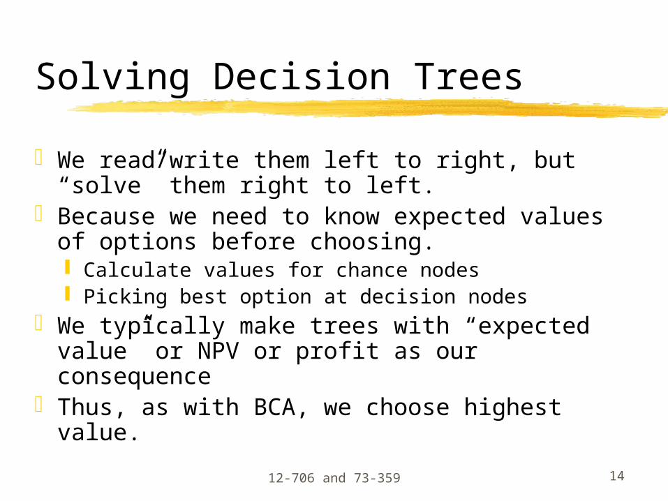
Solving Decision Trees

We read/write them left to right, but “solve” them right to left.

Because we need to know expected values of options before choosing. Calculate values for chance nodes Picking best option at decision nodes

We typically make trees with “expected value” or NPV or profit as our consequence

Thus, as with BCA, we choose highest value.

12-706 and 73-359 15

Texaco vs. Pennzoil

Counteroffer

$5 Billion

Texaco

Counteroffer

$3 Billion

Refuse

Settlement Amount ($ Billion)

Accept $2 Billion 2

Texaco Accept $5 Billion

5

Texaco Refuses

Counteroffer

Final Court

Decision

10.3

5

0

Final Court

Decision

10.3

5

0

Accept $3 Billion3

(0.17)

(0.5)

(0.33)

(0.2)

(0.5)

(0.3)

(0.2)

(0.5)

(0.3)

12-706 and 73-359 16

To Solve the Tree

Solve from right to left:At chance node multiply monetary value

to probability and add them.At choice node choose highest value.

EMV for Simple Texaco vs. Pennzoil Tree:$4.63 Billion

12-706 and 73-359 17

Risk Profiles

Risk profile shows a distribution of possible payoffs associated with particular strategies.

A strategy is what you plan to do going in to the decision. Holds your plans constant, allows chances to occur Only eliminate things YOU wouldn’t do, not things

“they” might not do.

Its not just finding the NPV of a branch.

12-706 and 73-359 18

Risk Profiles (cont.)

Let’s think about the “subset” of the Texaco decision tree where we are only curious about the uncertainty/risk profile associated with various strategies to consider.

These represent the riskiness of each option There are only 3 “decision strategies” in the base

Texaco case:Accept the $2 billion offer (topmost branch of 1st dec.

node)Counteroffer $5 Billion, but plan to refuse counteroffer

(lower branch of 1st node, upper branch of second)Counteroffer $5B, but plan to accept counteroffer (lower

branch of both decision nodes)

12-706 and 73-359 19

Texaco vs. Penzoil, Again

Risk Profile for "Accept to $2 Billion"

0%

100%

0% 0% 0% 0% 0% 0% 0% 0% 0%0%

20%

40%

60%

80%

100%

120%

0 1 2 3 4 5 6 7 8 9 10 11

x ($ Billion)

Chance that Settlement Equals X

Risk profile for “Accept $2 Billion” is obvious - get $2B with 100% chance.

12-706 and 73-359 20

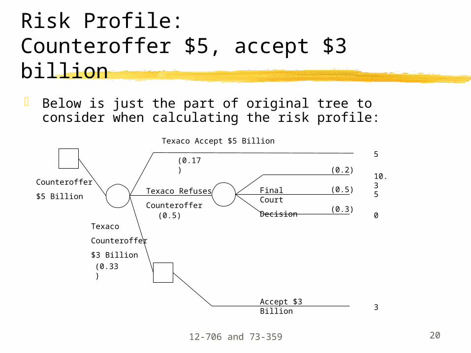
Risk Profile: Counteroffer $5, accept $3 billion Below is just the part of original tree to consider when

calculating the risk profile:

Counteroffer

$5 Billion

Texaco

Counteroffer

$3 Billion

Texaco Accept $5 Billion

5

Texaco Refuses

Counteroffer

Final Court

Decision

10.3

5

0

Accept $3 Billion3

(0.17)

(0.5)

(0.33)

(0.2)

(0.5)

(0.3)

12-706 and 73-359 21

Texaco vs. Pennzoil, continued

Risk Profile for "Counteroffer $5 Billion, Accept Texaco's $3 Billion Counteroffer"

15%

0%

33%

0%

42%

0% 0% 0% 0%

10%

0%0%

5%

10%

15%

20%

25%

30%

35%

40%

45%

0 1 2 3 4 5 6 7 8 9 10 11

x ($ Billion)

Chance that Settlement Equals x

Risk Profile for "Counteroffer $5 Billion, Reject Texaco's $3 Billion Counteroffer"

25%

0% 0% 0% 0%

59%

0% 0% 0% 0%

17%

0%0%

10%

20%

30%

40%

50%

60%

70%

0 1 2 3 4 5 6 7 8 9 10 11

x ($ Billion)

Chance that Settlement Equals x

12-706 and 73-359 22

Cumulative Risk Profiles

Graphs of cumulative distributions Percent chance that “payoff is less than

x”Cumulative Risk Profile for 3 Options in Texaco Case

0%

20%

40%

60%

80%

100%

120%

0 2 4 6 8 10 12

x ($billion)

Chance that payoff is less or equal to

x

Counteroffer $5 Billion, Accept Texaco's$3 Billion CounterofferAccept $2 Billion

Counteroffer $5 Billion, Refuse Texaco's$3 Billion Counteroffeer

12-706 and 73-359 23

Dominance

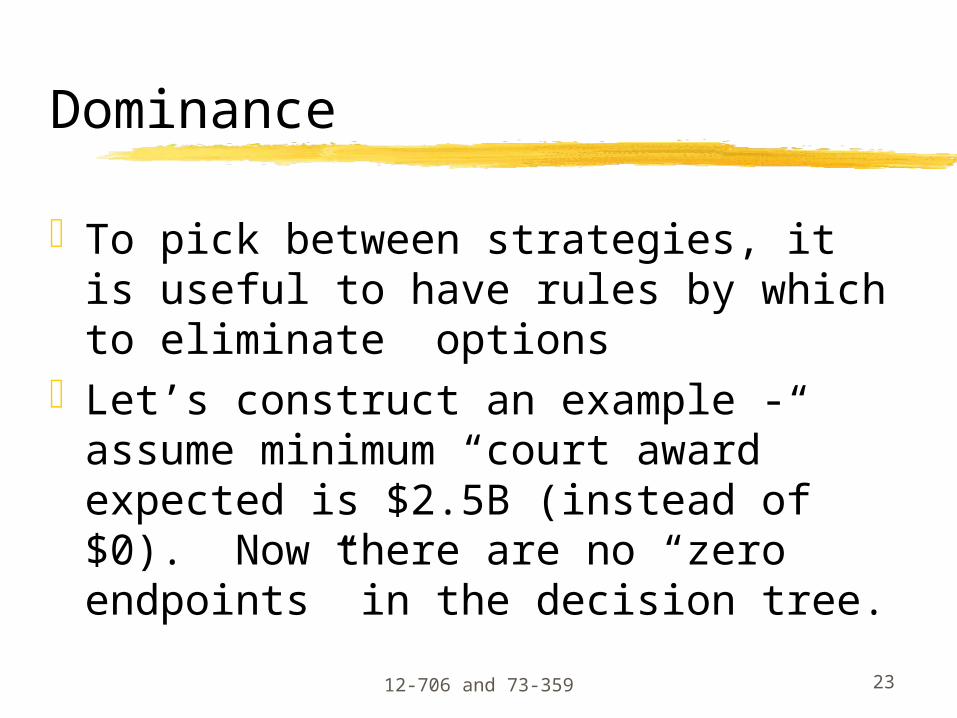
To pick between strategies, it is useful to have rules by which to eliminate options

Let’s construct an example - assume minimum “court award” expected is $2.5B (instead of $0). Now there are no “zero endpoints” in the decision tree.

12-706 and 73-359 24

Dominance Example

CRP below for 2 strategies shows “Accept $2 Billion” is dominated by the other.

0%

20%

40%

60%

80%

100%

120%

0 2 4 6 8 10 12

x ($billion)

Chance that payoff is less or equal to x

12-706 and 73-359 25

Next Class

Value of Information.

Facility Case Due