02 review of mathematicsstrana.donga.ac.kr/lecture/fem/pdf/fem_note.pdf · this lecture note has...

Department of Civil Engineering, DAU

Structural Analysis Lab.

This lecture note has been reproduced and distributed by courtesy by Prof. Hae Sung Lee, http://strana.snu.ac.kr

Review of Mathematics - Approximation of Functions -

≅ δ




� Discretization

)()(1

XX ∑=

=n

iii gaf υ∈∀ )(Xf where gi are the basis functions of υ.

� Approximations

)()()()(11

XXXX ∑∑==

=≈=

m

iii

hn

iii gafgaf where nm ≤

� Fundamental Questions

- What is the best approximation?

- How can we calculate ai that represents the best approximation?

� Summation Notation: Repeated indices denote summation ii

m

iii baba =∑

=1

.




� Norms of Functions: A measure of a function space

A function space υ is said to be a normed space if to every υ∈f there associated a

nonnegative real number f , called the norm of f, in a such way that

- 0=f if and only if 0≡f

- ff || α=α for any real number α.

- gfgf +≤+

Every normed space may be regarded as a metric space, in which the distance between any

two elements in the space is measured by the defined norm. Various types of norm can be

defined for a function space. Among them the following norms are important.

- L1 norm: ∫=

VL

dVff1

- L2 norm: 2/12

)(2

∫=

VL

dVff

- H1 norm:

2/12))((1 ∫ ∇⋅∇+=

VH

dVffff




� General Ideas for the Best Approximation

Let’s find out an approximate function that is closest to the given function by use of a norm

defined in the function space. If this is the case, the characteristics of an approximation

method depend on those of the norm used in the approximation.

� Least Square Error Minimization

Error: hffe −=

Minimize ∫ −=−==Π

V

h

L

h

LdVffffe

222

)(2

1

2

1

2

1

22

FKa ===−=−=

−=−=∂

∂−=

∂

Π∂

∑∫∑∫

∫∫ ∑∫∫

==

=

or ,,1for 0

)()(

11

1

mkFaKfdVgadVgg

fdVgdVaggdVgffdVa

fff

a

ki

m

iki

V

ki

m

i V

ik

V

k

V

m

iiik

V

kh

V k

hh

k

L

If the basis functions are orthogonal, K becomes diagonal.




� Variation of a function

- The variation of a function means a possible change in the function for the fixed x.

� Variational Calculus

- if ii gaf = ii gaf δ=δ or i

i

aa

ff δ

∂

∂=δ .

- ff

Fa

a

f

f

Fa

a

FFfF i

i

i

i

δδδδ∂

∂=

∂

∂

∂

∂=

∂

∂= : )(

- hfhf δ+δ=+δ )( , hffhfh δδδ +=)(

- , )()(dx

fda

a

f

dx

da

dx

df

adx

dfi

i

i

i

δ=δ

∂

∂=δ

∂

∂=δ ∫∫∫∫ δ=δ

∂

∂=δ

∂

∂=δ fdxdxa

a

fafdx

afdx i

i

i

i

f

δf

Variation of a function




� Minimization by Variational Calculus

Min ∫ −=Π

lhh

dxfff0

2)(2

1)(

k

k

k

l

k

hh

lhh

lh

lhh

aa

adxa

fff

dxfffdxffdxfff

δ∂

Π∂=δ

∂

∂−=

δ−=−δ=−δ=Πδ

∫

∫∫∫

0

00

2

0

2

)(

)()(2

1))(

2

1()(

Min k

lhh

adxfff δδ possible allfor 0)(2

1)(

0

2=Π⇔−=Π ∫

� Euler Equation

Min ka

dxxffFfk

l

allfor 0),,()(0

=∂

Π∂⇒′=Π ∫

∫

∫∫∫∫

′∂

∂−

∂

∂+

′∂

∂=

′′∂

∂+

∂

∂=

∂

′∂

′∂

∂+

∂

∂

∂

∂=

∂

∂=′

∂

∂=

∂

Π∂

l

kk

l

k

l

kk

l

kk

l

k

l

kk

dxgf

F

dx

dg

f

Fg

f

F

dxgf

Fg

f

Fdx

a

f

f

F

a

f

f

Fdx

a

FdxxffF

aa

00

0000

)(

)()(),,(




In case the basis functions vanish at the boundary, then

0 allfor 0)(0

=′∂

∂−

∂

∂⇔=

′∂

∂−

∂

∂=

∂

Π∂∫

f

F

dx

d

f

Fkdxg

f

F

dx

d

f

F

a

l

k

k

∫∫∫ δ′∂

∂−δ

∂

∂+δ

′∂

∂=′δ

′∂

∂+δ

∂

∂=′δ=Πδ

llll

dxff

F

dx

df

f

Ff

f

Fdxf

f

Ff

f

FdxxffFf

0000

)()(),,()(

In case the variation vanishes at the boundaries, then

k

k

k

l

k

l

aa

adxgf

F

dx

d

f

Ffdx

f

F

dx

d

f

Fδ

∂

Π∂=δ

′∂

∂−

∂

∂=δ

′∂

∂−

∂

∂=Πδ ∫∫

00

)()(

Therefore,

Min 0=Πδ⇔Π




� Example 1

Min ∫ ′+=Π

2

1

2)(1)(

x

x

dxyy subject to 11)( yxy = , 22 )( yxy =

0))(1( 2/12=′+′−=

′∂

∂−

∂

∂ −yy

dx

d

f

F

dx

d

f

F

0))(1())(1

)(1())(1(

))(1)(2

1())(1())(1(

2/32

2

22/12

2/322/122/12

=′+′′=′+

′−′+′′=

′′′′+−′+′+′′=′+′

−−

−−−

yyy

yyy

yyyyyyyydx

d

baxyy +=→=′′ 0 . By applying BC, 12

2112

12

120xx

yxyxx

xx

yyyy

−

−+

−

−=→=′′

� Example 2

Min ∫ −′=Π

l

dxufuu0

2))(

2

1()( subject to 0)0( =u , 0)( =lu

00))(2

1(

2=+′′→=′′−−=′−−=′

′∂

∂−−=

′∂

∂−

∂

∂fuufu

dx

dfu

udx

df

u

F

dx

d

u

F




Principle of Minimum Potential Energy vs

Principle of Virtual Work

(1-D elliptic differential equation)




� Problem Definition

0)()0( ,0 02

2

==<<=+ luulxfdx

ud

� Approximation – Discretization

∑=

=

m

iii

hgau

1

where 0)()0( == luuhh

� Residuals

Equation Residual : lxfdx

udR

h

E <<≠+= 0 02

2

Function Residual : lxuuRh

F <<≠−= 0 0

� Error Estimator :

∫∫ +−==Π

l hh

l

EFR

dxfdx

uduudxRR

02

2

0

))((




� Least Square Error

))((2

1))((

2

1))((

2

1

))((2

1))((

2

1

000

02

2

2

2

02

2

∫∫

∫∫

−−=−−−−−=

−−=+−=Π

l hhl hhl

hh

l hh

l hhR

dxdx

du

dx

du

dx

du

dx

dudx

dx

du

dx

du

dx

du

dx

du

dx

du

dx

duuu

dxdx

ud

dx

uduudxf

dx

uduu

� Energy Functional – Total potential Energy

RRl

hl hhl

l hhl

hh

lh

lh

lhl

h

lh

hh

hl hhR

Cfdxudxdx

du

dx

duufdx

dxdx

du

dx

du

dx

duudxu

dx

udu

dx

du

dx

duudxfuuf

dxfudx

uduuf

dx

ududxf

dx

uduu

Π+=−+=

+−+−+−=

−−+=+−=Π

∫∫∫

∫∫∫

∫∫

)2

1(

2

1

})({2

1

)(2

1))((

2

1

000

0002

2

000

02

2

2

2

02

2

� Minimization Problems

RRLSRΠ↔Π⇔Π Min Min Min w.r.t.

hhu υ∈

ΠLS

−f




� RR

ΠMin : Rayleigh-Ritz Method or Principle of Minimum Potential Energy

- 1st Order Necessary Condition of Minimization Problem

FKa =→==−=−=

−=

−=∂

Π∂

∑∫∑∫

∫ ∑∫ ∑∑

∫∫

==

===

mkFaKfdxgadxdx

dg

dx

dg

fdxgada

ddx

dx

dga

dx

dga

da

d

fdxda

dudx

dx

du

dx

du

da

d

a

m

ikiki

l

k

m

ii

lik

l m

iii

k

l m

i

ii

m

i

ii

k

l

k

hl hh

kk

RR

,,1for 0

)())((

)(

101 0

0 10 11

00

L

� 0=ΠδRR : Variational Principle or Principle of Virtual Work

�

0)()( 0)(

)(

)2

1(

1 1

1 01 0

000000

=−δ→=−δ=

−δ=

δ−δ

=δ−δ=−δ=Πδ

∑ ∑

∑ ∫∑∫

∫∫∫∫∫∫

= =

= =

FKaaT

m

k

m

ikikik

m

k

l

k

m

ii

lik

k

lh

l hhlh

l hhlh

l hhRR

FaKa

fdxgadxdx

dg

dx

dga

fdxudxdx

du

dx

udfdxudx

dx

du

dx

dufdxudx

dx

du

dx

du




Finite Element Formulation & Constant

Strain Triangle (CST) Element




� Interpolation and Shape Functions

To interpolate is to devise a continuous function that satisfies prescribed conditions at a finite

number of points.

in

i

i xa∑=

=

0

φ or xa=φ

in which ),,,,1( 2 nxxx L=x and T

naaaa ),,,,( 210 L=a .

where n = 1 for linear interpolation, n = 2 for quadratic interpolation, and so on.

The ai can be expressed in terms of nodal values of φ, which appear at known values of x as

follows:

Aa=eφφφφ

where each row of A is x evaluated at the appropriate nodal location.

eφφφφN=φ where ),,( 21

1LNN==

−xAN .

An individual Ni in matrix N is called a shape function or a basis function.




� Example of Shape Functions (1-D)




� Formulas for Element Stiffness Matrices Based on The Principle of Virtual Work

The principle of virtual work can be represented as the following equation:

∫∫∫ +=et

ee S

T

V

T

V

TdSdVdV tubu δδδ σσσσεεεε ( )

where ),,( wvuT

δδδδ =u and should be admissible virtual displacement. Here an admissible

displacement does not violate compatibility or displacement boundary conditions. b and t

denote body forces and tractions on a surface boundary.

� Interpolation of Displacement

Let displacements u be interpolated over an element such that

eNuu = where ),,( wvu=u

and eu represents the nodal displacement DOF of an element.

Strains can be expressed by differentiating the interpolated displacements as follows:

eBu=εεεε where NB ∂= (for differential operator ∂, refer to Eq.3.1-9 in the textbook)




Then, the virtual displacements and strains can be represented as,

euNu δδ = and e

uBδδ =εεεε

Substituting the above equation into the Eq. ( ) representing the principle of virtual work, Eq.

( ) becomes

0)()( =

−− ∫∫∫

et

eeS

T

V

Te

V

TTedSdVdV tNbNuCBBuδ ( )

Eq.( ) must be satisfied for any admissible virtual displacement dd. Therefore, Eq.( )

yields the element stiffness equation as follows:

eeefuk =

where the element stiffness ∫=e

V

TedVCBBk and the consistent nodal force vector

∫∫ +=et

e S

T

V

T

e dSdVr tNbN




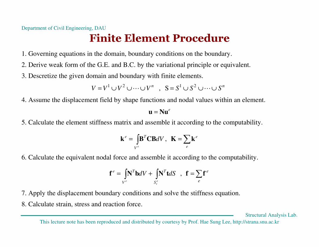
Finite Element Procedure

1. Governing equations in the domain, boundary conditions on the boundary.

2. Derive weak form of the G.E. and B.C. by the variational principle or equivalent.

3. Descretize the given domain and boundary with finite elements.

S , 2121 nn

SSSVVVV ∪∪∪=∪∪∪= LL

4. Assume the displacement field by shape functions and nodal values within an element.

eNuu =

5. Calculate the element stiffness matrix and assemble it according to the computability.

dVe

V

Te

∫= CBBk , ∑=

e

ekK

6. Calculate the equivalent nodal force and assemble it according to the computability.

dSdVet

e S

T

V

Te

∫∫ += tNbNf , ∑=

e

eff

7. Apply the displacement boundary conditions and solve the stiffness equation.

8. Calculate strain, stress and reaction force.




Finite Element Programming (Linear Static case)

Input

Preprocessing

Calculation of Element stiffness matrix and Load Vector

Assembling E.S.M and E.L.V.

Solve Global SE

Post-processing

Loop over all elements

Global Stiffness Matrix

and Load Vector

- Assemble Nodal Load Vector - Cal. of Destination Array - Cal. of Band width

Cal. Strain & Stress

Cal of Reaction Force

Display

Gauss Elimination Band solver Decomposition, etc




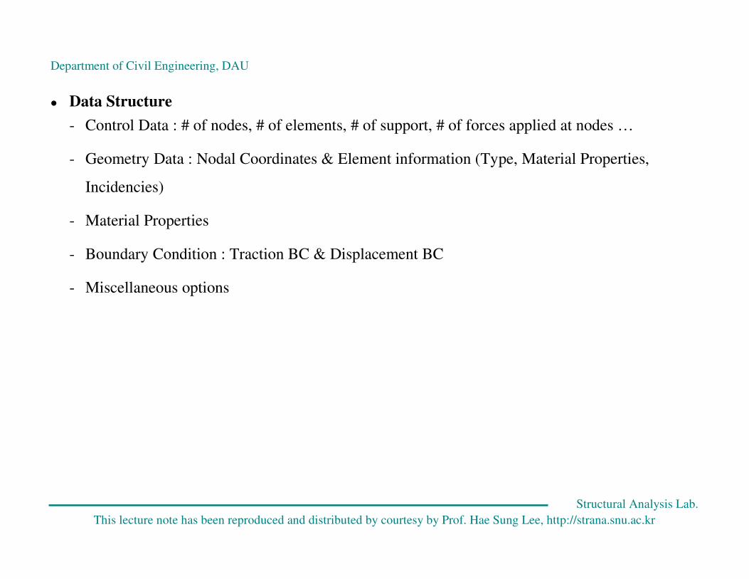
� Data Structure

- Control Data : # of nodes, # of elements, # of support, # of forces applied at nodes …

- Geometry Data : Nodal Coordinates & Element information (Type, Material Properties,

Incidencies)

- Material Properties

- Boundary Condition : Traction BC & Displacement BC

- Miscellaneous options




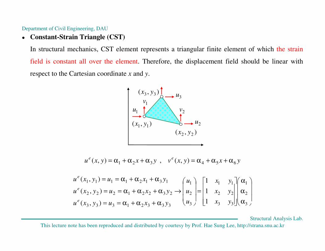
� Constant-Strain Triangle (CST)

In structural mechanics, CST element represents a triangular finite element of which the strain

field is constant all over the element. Therefore, the displacement field should be linear with

respect to the Cartesian coordinate x and y.

yxyxvyxyxuee

654321 ),( , ),( α+α+α=α+α+α=

33321333

23221222

13121111

),(

),(

),(

yxuyxu

yxuyxu

yxuyxu

e

e

e

α+α+α==

α+α+α==

α+α+α==

α

α

α

=

→

3

2

1

33

22

11

3

2

1

1

1

1

yx

yx

yx

u

u

u

1u

1v

2u

2v

3u

),( 11 yx

),( 22 yx

),( 33 yx




∆=

=

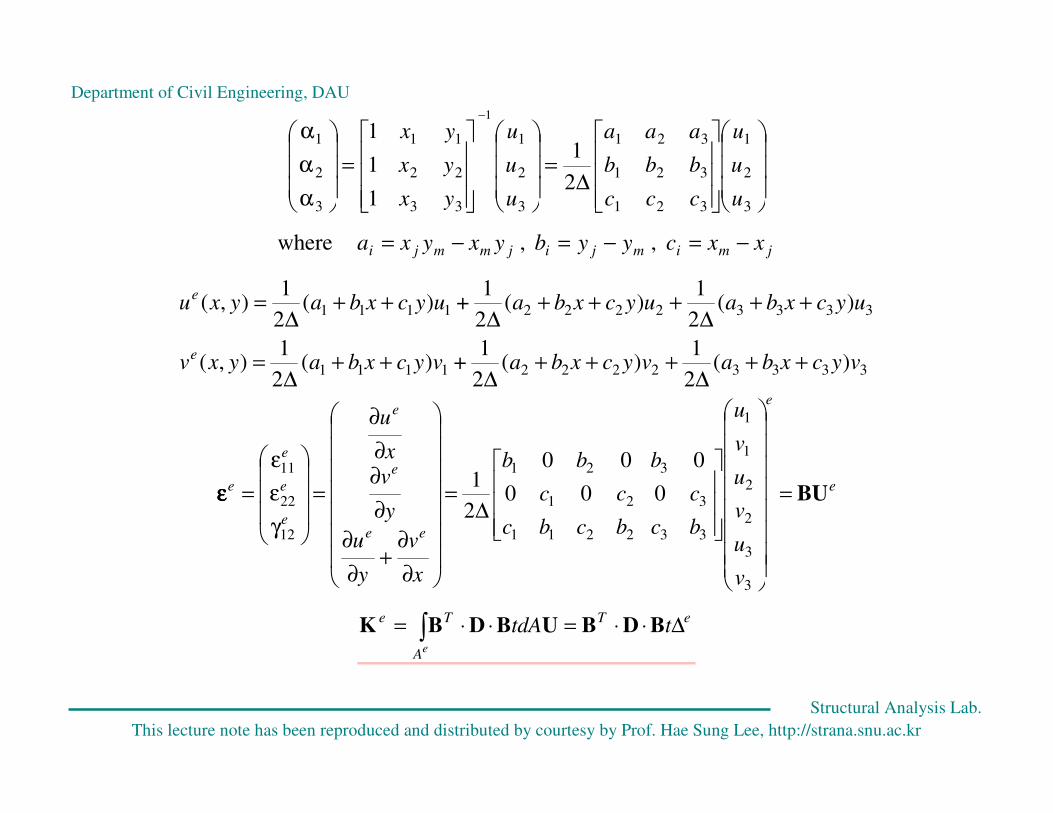
α

α

α−

3

2

1

321

321

321

3

2

1

33

22

11

3

2

1

2

1

1

1

11

u

u

u

ccc

bbb

aaa

u

u

u

yx

yx

yx

where jmimjijmmji xxcyybyxyxa −=−=−= , ,

333322221111

333322221111

)(2

1)(

2

1 +)(

2

1),(

)(2

1)(

2

1 +)(

2

1),(

vycxbavycxbavycxbayxv

uycxbauycxbauycxbayxu

e

e

++∆

+++∆

++∆

=

++∆

+++∆

++∆

=

e

e

ee

e

e

e

e

e

e

v

u

v

u

v

u

bc

c

b

bc

c

b

bc

c

b

x

v

y

u

y

v

x

u

BU=

∆=

∂

∂+

∂

∂

∂

∂

∂

∂

=

γ

ε

ε

=

3

3

2

2

1

1

33

3

3

22

2

2

11

1

1

12

22

11

0

0

0

0

0

0

2

1εεεε

∫ ∆⋅⋅=⋅⋅=eA

eTTettdA BDBUBDBK




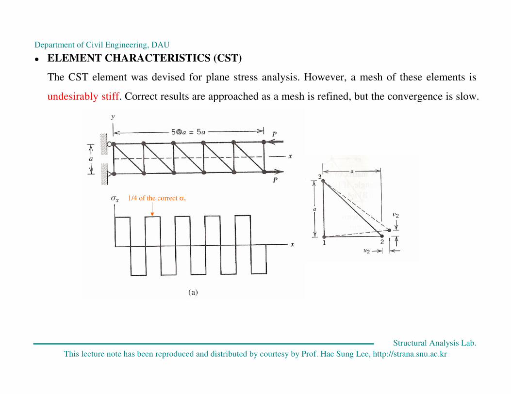
� ELEMENT CHARACTERISTICS (CST)

The CST element was devised for plane stress analysis. However, a mesh of these elements is

undesirably stiff. Correct results are approached as a mesh is refined, but the convergence is slow.

1/4 of the correct σx




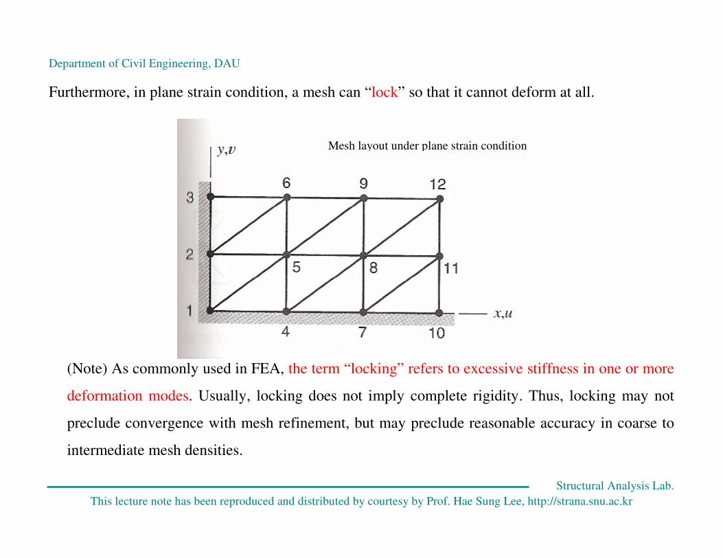
Furthermore, in plane strain condition, a mesh can “lock” so that it cannot deform at all.

(Note) As commonly used in FEA, the term “locking” refers to excessive stiffness in one or more

deformation modes. Usually, locking does not imply complete rigidity. Thus, locking may not

preclude convergence with mesh refinement, but may preclude reasonable accuracy in coarse to

intermediate mesh densities.

Mesh layout under plane strain condition




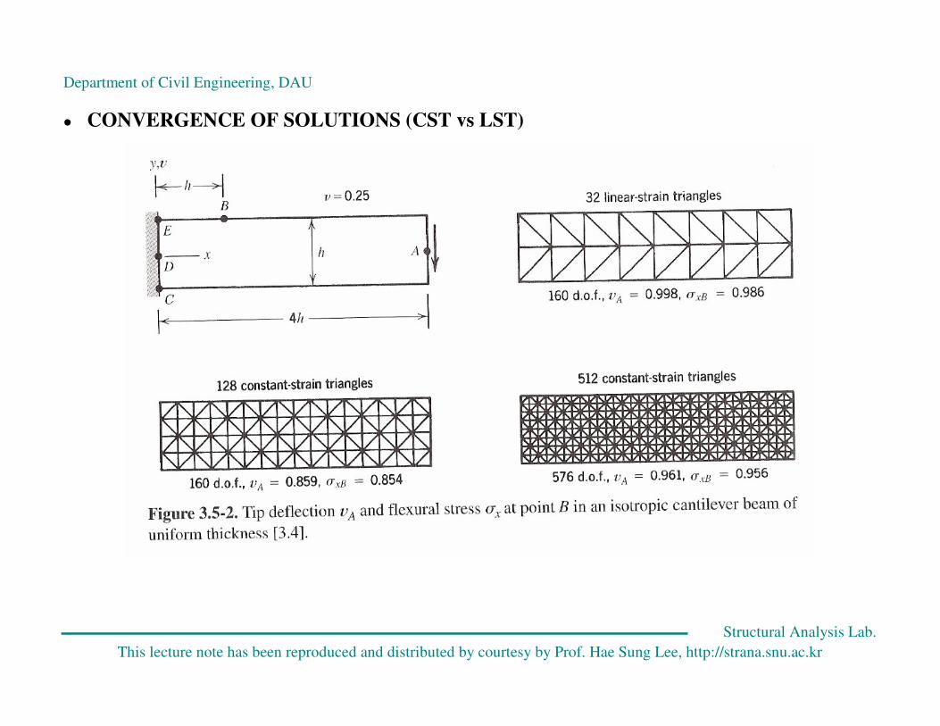
� CONVERGENCE OF SOLUTIONS (CST vs LST)

Mesh layout under plane strain condition




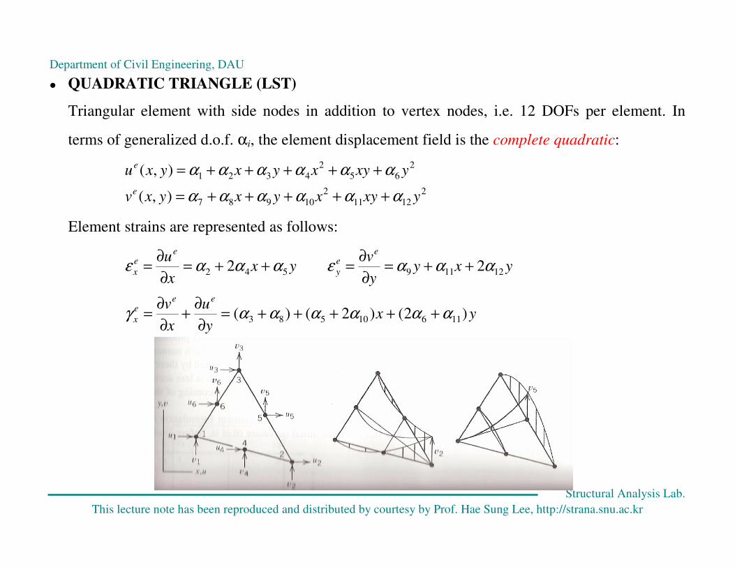
� QUADRATIC TRIANGLE (LST)

Triangular element with side nodes in addition to vertex nodes, i.e. 12 DOFs per element. In

terms of generalized d.o.f. αi, the element displacement field is the complete quadratic:

2

1211

2

10987

2

65

2

4321

),(

),(

yxyxyxyxv

yxyxyxyxu

e

e

αααααα

αααααα

+++++=

+++++=

Element strains are represented as follows:

yxy

u

x

v

yxyy

vyx

x

u

eee

x

ee

y

ee

x

)2()2()(

22

11610583

12119542

ααααααγ

αααεαααε

+++++=∂

∂+

∂

∂=

++=∂

∂=++=

∂

∂=




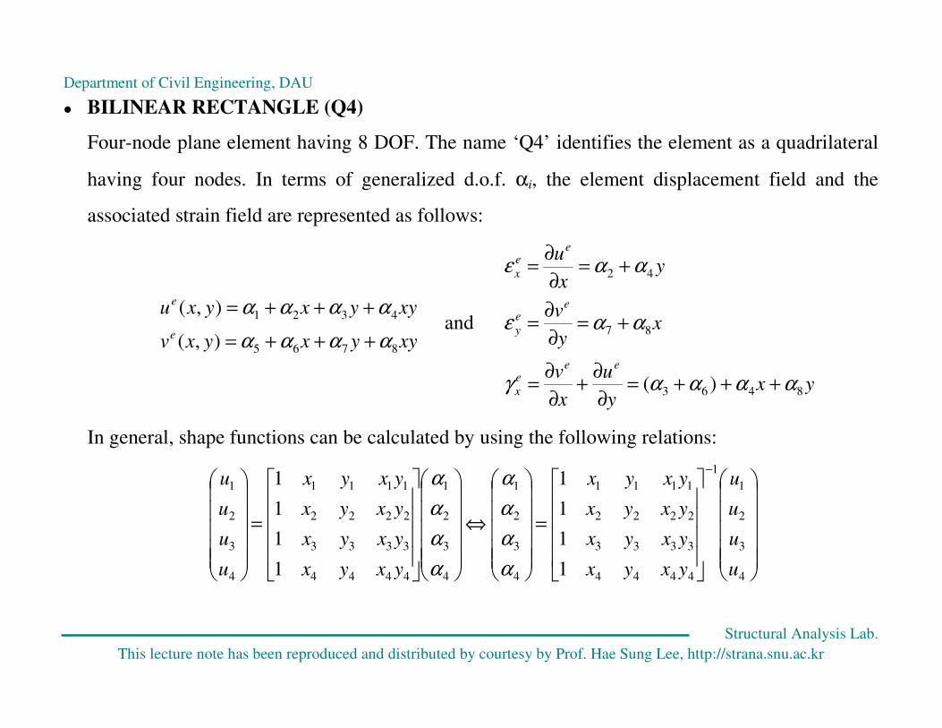
� BILINEAR RECTANGLE (Q4)

Four-node plane element having 8 DOF. The name ‘Q4’ identifies the element as a quadrilateral

having four nodes. In terms of generalized d.o.f. αi, the element displacement field and the

associated strain field are represented as follows:

xyyxyxv

xyyxyxu

e

e

8765

4321

),(

),(

αααα

αααα

+++=

+++= and

yxy

u

x

v

xy

v

yx

u

eee

x

ee

y

ee

x

8463

87

42

)( ααααγ

ααε

ααε

+++=∂

∂+

∂

∂=

+=∂

∂=

+=∂

∂=

In general, shape functions can be calculated by using the following relations:

=

⇔

=

−

4

3

2

1

1

4444

3333

2222

1111

4

3

2

1

4

3

2

1

4444

3333

2222

1111

4

3

2

1

1

1

1

1

1

1

1

1

u

u

u

u

yxyx

yxyx

yxyx

yxyx

yxyx

yxyx

yxyx

yxyx

u

u

u

u

α

α

α

α

α

α

α

α




=

⇔

=

−

4

3

2

1

1

4444

3333

2222

1111

4

3

2

1

4

3

2

1

4444

3333

2222

1111

4

3

2

1

1

1

1

1

1

1

1

1

v

v

v

v

yxyx

yxyx

yxyx

yxyx

yxyx

yxyx

yxyx

yxyx

v

v

v

v

α

α

α

α

α

α

α

α

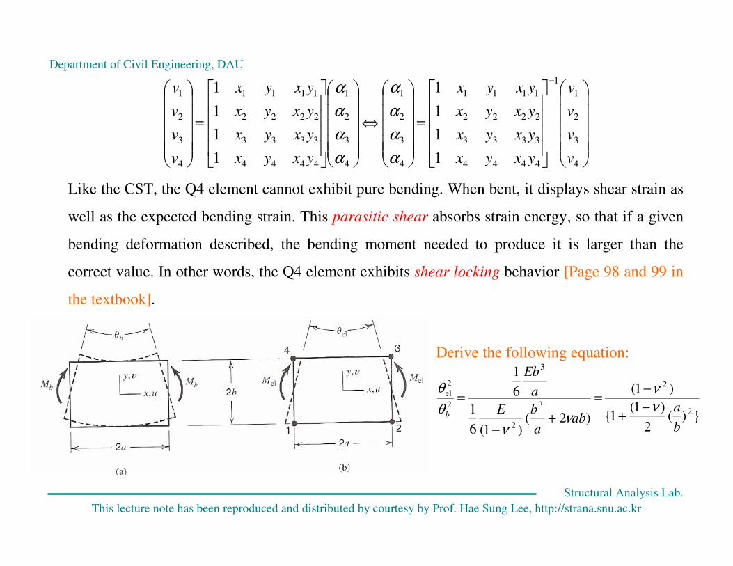
Like the CST, the Q4 element cannot exhibit pure bending. When bent, it displays shear strain as

well as the expected bending strain. This parasitic shear absorbs strain energy, so that if a given

bending deformation described, the bending moment needed to produce it is larger than the

correct value. In other words, the Q4 element exhibits shear locking behavior [Page 98 and 99 in

the textbook].

Derive the following equation:

})(2

)1(1{

)1(

)2()1(6

1

6

1

2

2

3

2

3

2

2

el

b

aab

a

bE

a

Eb

bν

ν

νν

θ

θ

−+

−=

+−

=




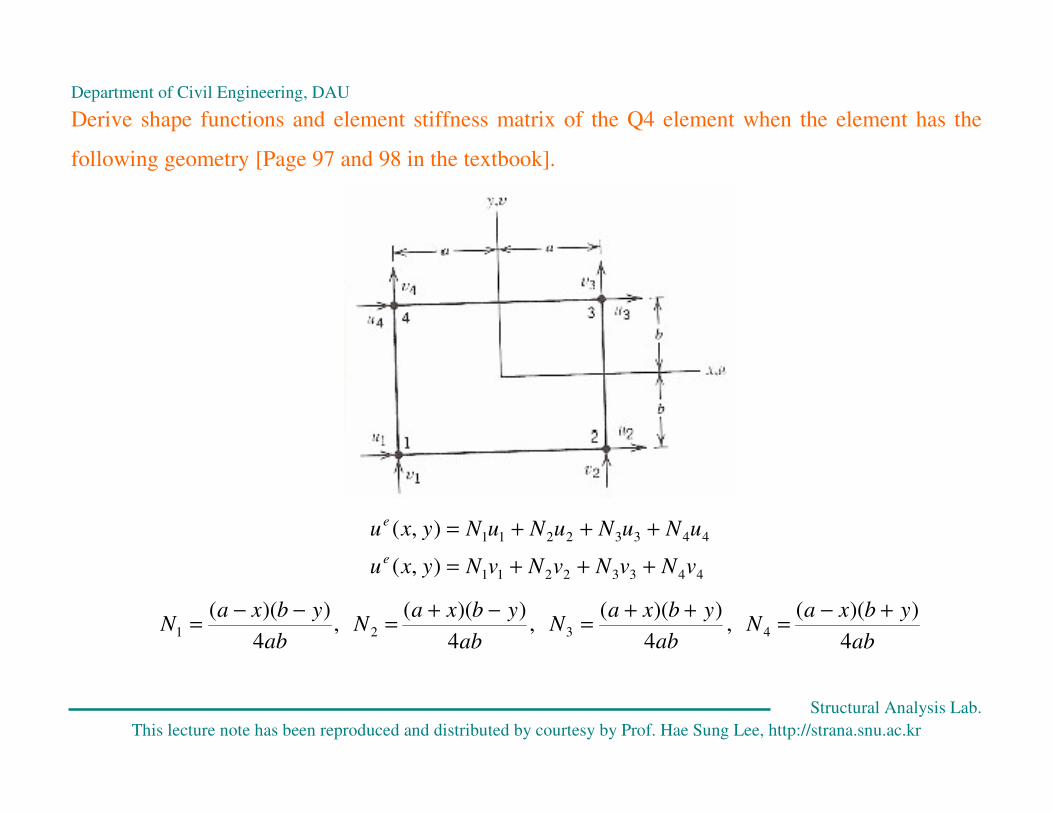
Derive shape functions and element stiffness matrix of the Q4 element when the element has the

following geometry [Page 97 and 98 in the textbook].

44332211

44332211

),(

),(

vNvNvNvNyxu

uNuNuNuNyxu

e

e

+++=

+++=

ab

ybxaN

4

))((1

−−= ,

ab

ybxaN

4

))((2

−+= ,

ab

ybxaN

4

))((3

++= ,

ab

ybxaN

4

))((4

+−=




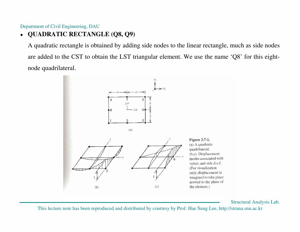
� QUADRATIC RECTANGLE (Q8, Q9)

A quadratic rectangle is obtained by adding side nodes to the linear rectangle, much as side nodes

are added to the CST to obtain the LST triangular element. We use the name ‘Q8’ for this eight-

node quadrilateral.




( )

dVE

dVE

dVE

dVE

dVU

V

xyyxyx

V

xyyyxxyx

Vxy

y

x

xyyxyx

Vxy

y

x

xyyx

V

T

el

∫

∫

∫

∫∫

−+++

−=

−++++

−=

−++

−=

−−==

}2

)1(2{

)1(2

1

}2

1)(){(

)1(2

1

2

1

)1(2

1

2

100

01

01

)1(2

1

2

1

222

2

2

2

2

2

γν

ενεεεν

γν

εενεενεεν

γ

ε

ε

γν

ενενεεν

γ

ε

ε

νν

ν

νγεεεεεεεεεε E




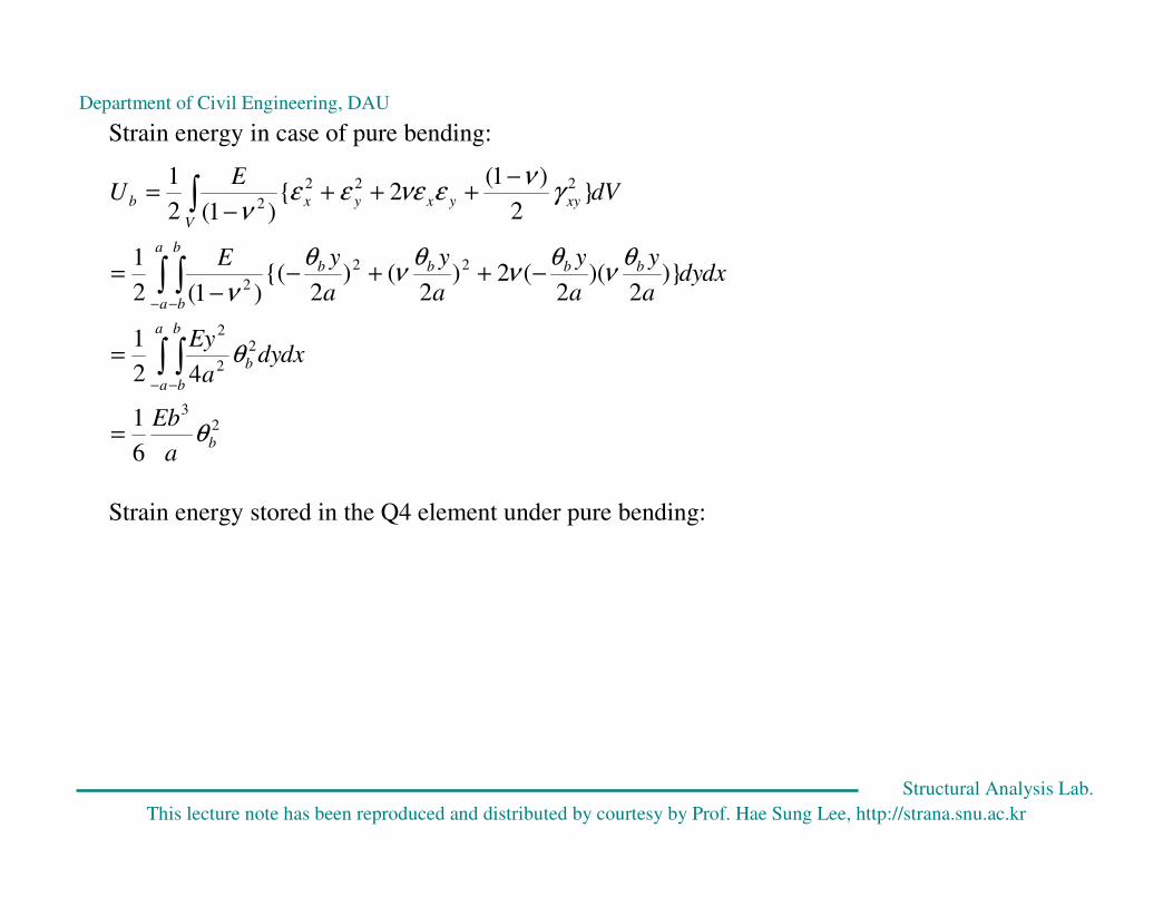
Strain energy in case of pure bending:

23

2

2

2

22

2

222

2

6

1

42

1

)}2

)(2

(2)2

()2

{()1(2

1

}2

)1(2{

)1(2

1

b

a

a

b

b

b

a

a

b

b

bbbb

V

xyyxyxb

a

Eb

dxdya

Ey

dxdya

y

a

y

a

y

a

yE

dVE

U

θ

θ

θν

θν

θν

θ

ν

γν

ενεεεν

=

=

−++−−

=

−+++

−=

∫ ∫

∫ ∫

∫

− −

− −

Strain energy stored in the Q4 element under pure bending:




2

el

3

2

2

el

3

2

3

2

2

el3

2

2

el

2

2

22

el

2

22

el

2

elel2el

2

222

2el

)2

)1((

)1(6

1}

3

2

3{

)1(2

1

}3

2)2(

42

)1(

3

2)2(

4{

)1(2

1

)42

)1(

4(

)1(2

1

)}2

)(2

(2

)1()

2{(

)1(2

1

}2

)1(2{

)1(2

1

θν

νθν

ν

θνθ

ν

θνθ

ν

θθνθ

ν

γν

ενεεεν

aba

bEab

a

bE

ab

a

ba

a

E

dxdya

x

a

yE

dxdya

x

a

x

a

yE

dVE

U

a

a

b

b

a

a

b

b

V

xyyxyx

−+

−=+

−=

−+

−=

−+

−=

−−−

+−−

=

−+++

−=

∫ ∫

∫ ∫

∫

− −

− −

})(2

)1(1{

)1(

)2()1(6

1

6

1

)2

)1((

)1(6

1

6

1

2

2

3

2

3

2

2

el

2

el

3

2

23

el

b

aab

a

bE

a

Eb

aba

bE

a

Eb

UU

b

b

b

ν

ν

νν

θ

θ

θν

νθ

−+

−=

+−

=

−+

−=

=


Structural Analysis Lab. This lecture note has been reproduced and distributed by courtesy by Prof. Hae Sung Lee, http://strana.snu.ac.kr

Isoparametric Formulations



Isoparametric Formulation Interpolation of Geometry

∑

∑

=

=

ηξ=ηξ++ηξ=

ηξ=ηξ++ηξ=

m

iiinm

m

iiinm

yNyNyNy

xNxNxNx

111

111

),(),(),(

),(),(),(

L

L

Natural (intrinsic) coordinate system

Actual coordinate system



ee

e

m

m

m

me

ee

yx

yxyx

NN

NN

NN

yx

XNx =

⎟⎟⎟⎟⎟⎟⎟⎟⎟

⎠

⎞

⎜⎜⎜⎜⎜⎜⎜⎜⎜

⎝

⎛

⎥⎦

⎤⎢⎣

⎡=⎟

⎟⎠

⎞⎜⎜⎝

⎛=

M

L 2

2

1

1

2

2

1

1

00

0

0

00

Interpolation of Displacement in a Parent Element

eee

ee

vu

UNu ),( ηξ=⎟⎟⎠

⎞⎜⎜⎝

⎛=

Derivatives of the Displacement Shape Functions

→⎟⎟⎟⎟

⎠

⎞

⎜⎜⎜⎜

⎝

⎛

∂∂∂∂

⎥⎥⎥⎥

⎦

⎤

⎢⎢⎢⎢

⎣

⎡

∂η∂

∂η∂

∂ξ∂

∂ξ∂

=⎟⎟⎟⎟

⎠

⎞

⎜⎜⎜⎜

⎝

⎛

∂η∂∂ξ∂

→

⎪⎪⎭

⎪⎪⎬

⎫

∂η∂

∂∂

+∂η∂

∂∂

=∂η∂

∂ξ∂

∂∂

+∂ξ∂

∂∂

=∂ξ∂

yNx

N

yx

yx

N

N

yy

Nxx

NN

yy

Nxx

NN

i

i

i

i

iii

iii



iixi

i

i

i

i

i

NNN

N

N

N

yx

yx

yNx

N

η−−

−

∇=∇⎟⎟⎟⎟

⎠

⎞

⎜⎜⎜⎜

⎝

⎛

∂η∂∂ξ∂

=⎟⎟⎟⎟

⎠

⎞

⎜⎜⎜⎜

⎝

⎛

∂η∂∂ξ∂

⎥⎥⎥⎥

⎦

⎤

⎢⎢⎢⎢

⎣

⎡

∂η∂

∂η∂

∂ξ∂

∂ξ∂

=⎟⎟⎟⎟

⎠

⎞

⎜⎜⎜⎜

⎝

⎛

∂∂∂∂

11

1

or JJ

XNJ ⋅∇=

⎥⎥⎥⎥

⎦

⎤

⎢⎢⎢⎢

⎣

⎡

⎥⎥⎥⎥

⎦

⎤

⎢⎢⎢⎢

⎣

⎡

∂η∂∂ξ∂

∂η∂∂ξ∂

∂η∂∂ξ∂

=

⎥⎥⎥⎥

⎦

⎤

⎢⎢⎢⎢

⎣

⎡

∂η∂

∂η∂

∂ξ∂

∂ξ∂

=

⎥⎥⎥⎥

⎦

⎤

⎢⎢⎢⎢

⎣

⎡

∂η∂

∂η∂

∂ξ∂

∂ξ∂

= ξ

==

==

∑∑

∑∑

mm

m

m

m

ii

im

ii

i

m

ii

im

ii

i

yx

yxyx

N

N

N

N

N

N

yNxN

yNxN

yx

yx

22

11

2

2

1

1

11

11

ML

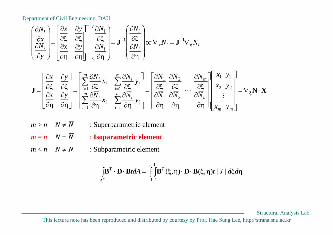
m > n NN ≠ : Superparametric element

m = n NN = : Isoparametric element

m < n NN ≠ : Subparametric element

∫ ∫∫− −

ηξηξ⋅⋅ηξ=⋅⋅1

1

1

1||),(),( ddJttdA T

A

T

e

BDBBDB



Bilinear Isoparametric Element

Shape functions in the parent coordinate system.

)),(),,(( )),(),,((

8765

4321

ξηα+ηα+ξα+α=ηξηξξηα+ηα+ξα+α=ηξηξ

yxvyxu

4321444434214444444

4321334333213333333

4321224232212222222

4321114131211111111

)),(),,((),()),(),,((),()),(),,((),(

)),(),,((),(

α−α+α−α=ηξα+ηα+ξα+α=ηξηξ==α+α+α+α=ηξα+ηα+ξα+α=ηξηξ==α−α−α+α=ηξα+ηα+ξα+α=ηξηξ==

α+α−α−α=ηξα+ηα+ξα+α=ηξηξ==

yxuyxuuyxuyxuuyxuyxuu

yxuyxuu

ξ

η

η=0.5

η=−0.5

ξ=0.5ξ=−0.5ξ=−0.5 ξ=0.5

η=0.5

η=−0.5

1 2

3

1 2

3 4 4



⎟⎟⎟⎟⎟

⎠

⎞

⎜⎜⎜⎜⎜

⎝

⎛

⎥⎥⎥⎥

⎦

⎤

⎢⎢⎢⎢

⎣

⎡

−−

−−−−

=

⎟⎟⎟⎟⎟

⎠

⎞

⎜⎜⎜⎜⎜

⎝

⎛

4

3

2

1

4

3

2

1

1111111111111111

αααα

uuuu

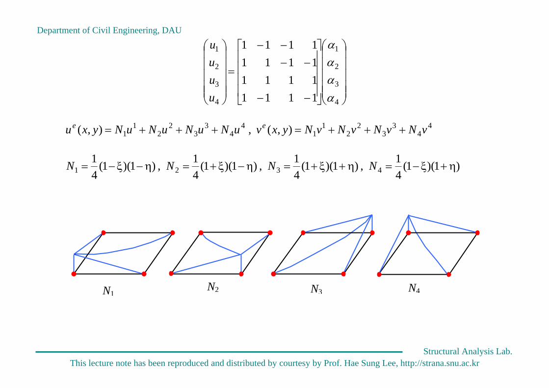
),( , ),( 4

43

32

21

14

43

32

21

1 vNvNvNvNyxvuNuNuNuNyxu ee +++=+++=

)1)(1(41 , )1)(1(

41 , )1)(1(

41 , )1)(1(

41

4321 η+ξ−=η+ξ+=η−ξ+=η−ξ−= NNNN

N1N2 N3 N4



Triangular Isoparametric Element

Area Coordinate System

1 , , , 3213

32

21

1 =α+α+α=α=α=αAA

AA

AA

Shape functions

- CST Element

332211 , , α=α=α= NNN

- LST Element

A3

A1 A2

1 2

3

α1 constant line

α2 constant line

α3 constant line



316325214

333222111

4 4 4)1(2 )1(2 )1(2

αα=αα=αα=−αα=−αα=−αα=

NNNNNN

Interpolation of Geometry

∑∑

∑∑

==

==

αα=ααα=

αα=ααα=

n

iii

n

iii

n

iii

n

iii

yNyNy

xNxNx

121

1321

121

1321

),(~),,(

),(~),,(

)(]~[~00~

~00~

)(1

1

1

1 ee

e

m

mn

ne

ee XN

yx

yx

NN

NN

yx

=

⎟⎟⎟⎟⎟⎟

⎠

⎞

⎜⎜⎜⎜⎜⎜

⎝

⎛

⎥⎦

⎤⎢⎣

⎡=⎟

⎟⎠

⎞⎜⎜⎝

⎛= MLX

Interpolation of Displacement in a Parent Element

)()],(~[)()],,([)( 21321eeee

e

ee UNUN

vu

u αα=ααα=⎟⎟⎠

⎞⎜⎜⎝

⎛=



Derivatives of the Displacement Shape Functions

ii

i

i

i

i

i

i

i

i

i

iii

iii

N

N

N

N

yx

yx

yNx

N

yNx

N

yx

yx

N

N

yy

Nxx

NN

yy

Nxx

NN

~

~

~

~

~

~

~

~

~

~

~~~

~~~

2

11

2

1

1

22

11

22

11

2

1

222

111

⎟⎟⎟⎟

⎠

⎞

⎜⎜⎜⎜

⎝

⎛

∂α∂∂α∂

=

⎟⎟⎟⎟

⎠

⎞

⎜⎜⎜⎜

⎝

⎛

∂α∂∂α∂

⎥⎥⎥⎥

⎦

⎤

⎢⎢⎢⎢

⎣

⎡

∂α∂

∂α∂

∂α∂

∂α∂

=

⎟⎟⎟⎟

⎠

⎞

⎜⎜⎜⎜

⎝

⎛

∂∂∂∂

→

⎟⎟⎟⎟

⎠

⎞

⎜⎜⎜⎜

⎝

⎛

∂∂∂∂

⎥⎥⎥⎥

⎦

⎤

⎢⎢⎢⎢

⎣

⎡

∂α∂

∂α∂

∂α∂

∂α∂

=

⎟⎟⎟⎟

⎠

⎞

⎜⎜⎜⎜

⎝

⎛

∂α∂∂α∂

→

⎪⎪⎭

⎪⎪⎬

⎫

∂α∂

∂∂

+∂α∂

∂∂

=∂α∂

∂α∂

∂∂

+∂α∂

∂∂

=∂α∂

−

−

J

or

iix NN ~~ 1α

− ∇=∇ J



XNJ ⋅∇=

⎥⎥⎥⎥

⎦

⎤

⎢⎢⎢⎢

⎣

⎡

⎥⎥⎥⎥

⎦

⎤

⎢⎢⎢⎢

⎣

⎡

∂α∂∂α∂

∂α∂∂α∂

∂α∂∂α∂

=

⎥⎥⎥⎥

⎦

⎤

⎢⎢⎢⎢

⎣

⎡

∂α∂

∂α∂

∂α∂

∂α∂

=

⎥⎥⎥⎥

⎦

⎤

⎢⎢⎢⎢

⎣

⎡

∂α∂

∂α∂

∂α∂

∂α∂

= α

==

==

∑∑

∑∑ ~

~

~

~

~

~

~

~~

~~

22

11

2

1

2

2

1

2

2

1

1

1

1 21 2

1 11 1

22

11

mm

m

m

m

ii

im

ii

i

m

ii

im

ii

i

yx

yxyx

N

N

N

N

N

N

yNxN

yNxN

yx

yx

ML




Numerical Integration




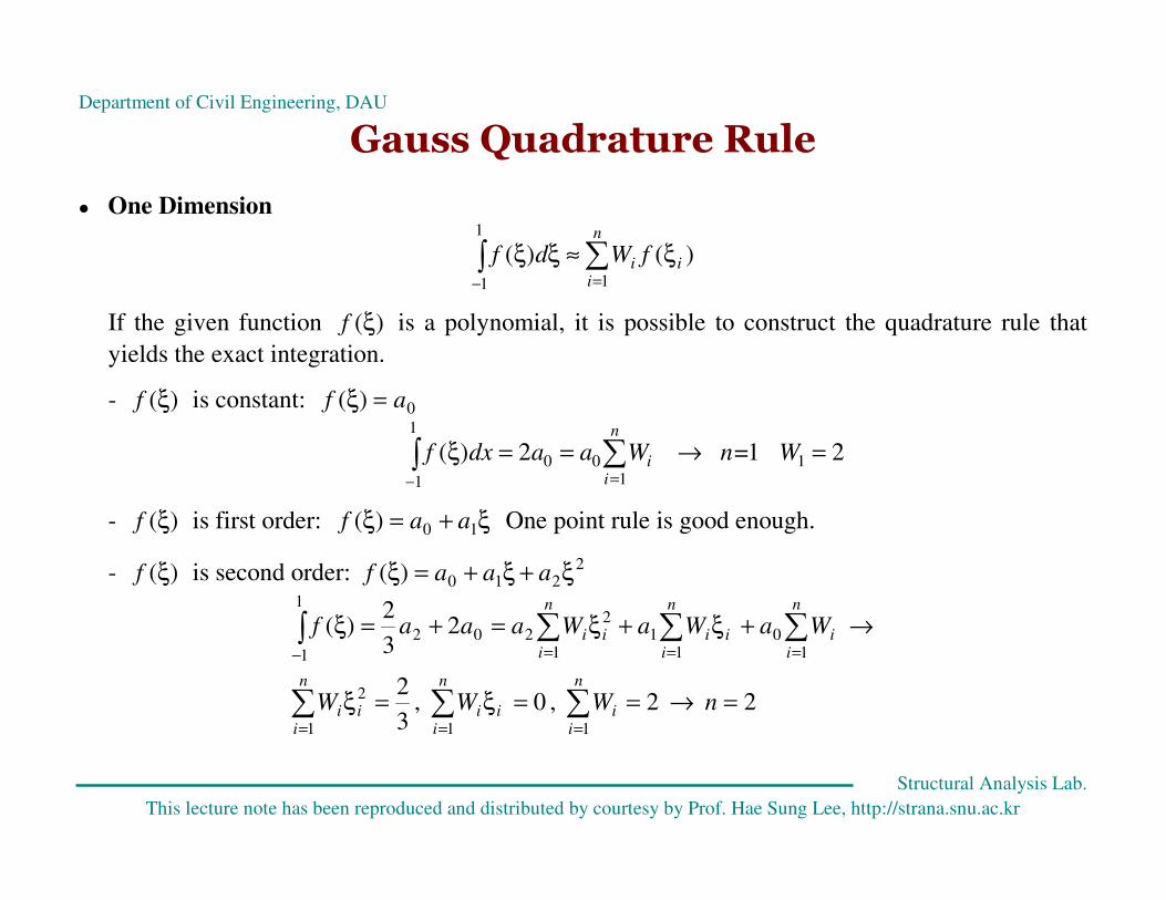
Gauss Quadrature Rule

� One Dimension

∫ ∑− =

ξ≈ξξ

1

1 1

)()(n

iii fWdf

If the given function )(ξf is a polynomial, it is possible to construct the quadrature rule that

yields the exact integration.

- )(ξf is constant: 0)( af =ξ

2 1 2)( 1

1

1 100 =→==ξ∫ ∑

− =

W n=Waadxfn

ii

- )(ξf is first order: ξ+=ξ 10)( aaf One point rule is good enough.

- )(ξf is second order: 2

210)( ξ+ξ+=ξ aaaf

2 2 , 0 , 3

2

23

2)(

111

2

1

1 10

11

1

2202

=→==ξ=ξ

→+ξ+ξ=+=ξ

∑∑∑

∫ ∑∑∑

===

− ===

nWWW

WaWaWaaaf

n

ii

n

iii

n

iii

n

ii

n

iii

n

iii




21211

1 , 0 ξ−=ξ=→=ξ∑=

WWWn

iii

3

1

3

22

222

222

222

211

2

1

2=ξ→=ξ=ξ+ξ=ξ∑

=

WWWWWi

ii

89626 02691 57735.01/3= 1 22 22221

2

1

=ξ→=→==+=∑=

WWWWWi

i

- )(ξf is third order: 3

32

210)( ξ+ξ+ξ+=ξ aaaaf Two point rule is enough.

- )(ξf is fourth order: 4

43

32

210)( ξ+ξ+ξ+ξ+=ξ aaaaaf

3 2 , 0 , 3

2 , 0 ,

5

2

23

2

5

2)(

111

2

1

3

1

4

10

11

1

22

1

33

1

44

1

1

024

=→==ξ=ξ=ξ=ξ

→+ξ+ξ+ξ+ξ=++=ξξ

∑∑∑∑∑

∑∑∑∑∑∫

=====

=====−

nWWWWW

WaWaWaWaWaaaadf

n

ii

n

iii

n

iii

n

iii

n

iii

n

ii

n

iii

n

iii

n

iii

n

iii

0 , , 0 , 0 2313111

3=ξξ−=ξ=→=ξ=ξ ∑∑

==

WWWWn

iii

n

iii

5

1

5

22 4

33433

433

411

3

1

4=ξ→=ξ=ξ+ξ=ξ∑

=

WWWWWi

ii




55555 55555 55555.0 , 41483 66692 77459.0

9

5 = , 5/3

3

1

3

22

33

33233

233

233

211

3

1

2

==ξ

=ξ→=ξ→=ξ=ξ+ξ=ξ∑=

W

WWWWWWi

ii

88888 88888 0.88888= 9

8 22 223321

3

1

=→=+=++=∑=

WWWWWWWi

i

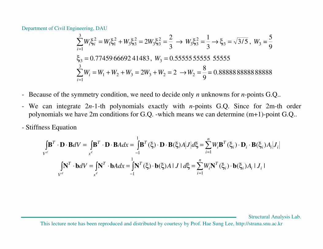
- Because of the symmetry condition, we need to decide only n unknowns for n-points G.Q..

- We can integrate 2n-1-th polynomials exactly with n-points G.Q. Since for 2m-th order

polynomials we have 2m conditions for G.Q. -which means we can determine (m+1)-point G.Q..

- Stiffness Equation

∑∫∫∫=−

ξ⋅⋅ξ=ξξ⋅⋅ξ=⋅⋅=⋅⋅

n

iiiiii

Ti

T

x

T

V

TJAWdJAAdxdV

ee 1

1

1

)()()()( BDBBDBBDBBDB

∑∫∫∫=−

ξ⋅ξ=ξξ⋅ξ=⋅=⋅

n

iiiii

Ti

T

x

T

V

TJAWdJAAdxdV

ee 1

1

1

||)()(||)()( bNbNbNbN




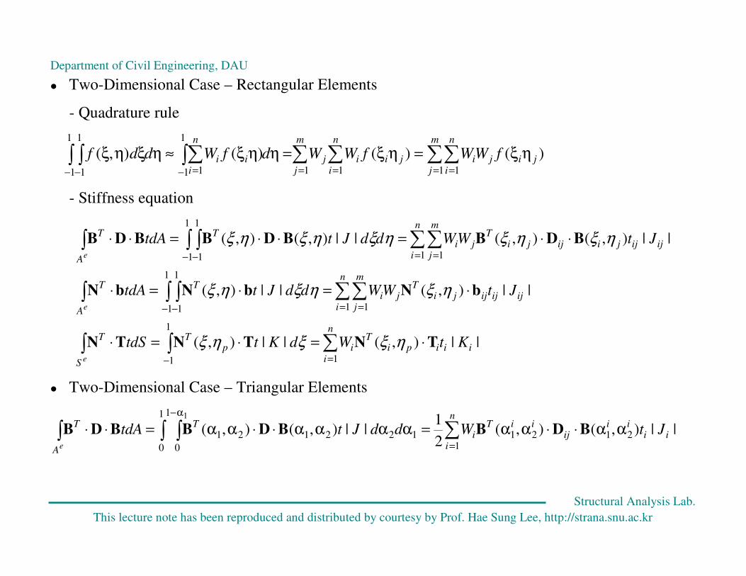
� Two-Dimensional Case – Rectangular Elements

- Quadrature rule

∑∑∑∑∫∑∫ ∫= ===− =− −

ηξ=ηξ=ηηξ≈ηξηξ

m

j

n

ijiji

n

ijii

m

jj

n

iii fWWfWWdfWddf

1 111

1

1 1

1

1

1

1

)()()(),(

- Stiffness equation

∑∫∫

∑∑∫ ∫∫

∑∑∫ ∫∫

=−

= =− −

= =− −

⋅=⋅=⋅

⋅=⋅=⋅

⋅⋅=⋅⋅=⋅⋅

n

iiiipi

Tip

T

S

T

n

i

m

jijijijji

Tji

T

A

T

n

i

m

jijijjiijji

Tji

T

A

T

KtWdKttdS

JtWWddJttdA

JtWWddJttdA

e

e

e

1

1

1

1 1

1

1

1

1

1 1

1

1

1

1

||),(||),(

||),(||),(

||),(),(||),(),(

TNTNTN

bNbNbN

BDBBDBBDB

ηξξηξ

ηξηξηξ

ηξηξηξηξηξ

� Two-Dimensional Case – Triangular Elements

∑∫ ∫∫=

α−

αα⋅⋅αα=αααα⋅⋅αα=⋅⋅

n

iii

iiij

iiTi

T

A

TJtWddJttdA

e 12121

1

0

1

0

122121 ||),(),(2

1||),(),(

1

BDBBDBBDB




Reduced Integration � Q8 element

27

26

254

23210

27

26

254

23210

ξη+ηξ+η+ξη+ξ+η+ξ+=

ξη+ηξ+η+ξη+ξ+η+ξ+=

bbbbbbbbv

aaaaaaaau

276431

276431 22 , 22 η+ξη+η+ξ+=

ξ∂

∂η+ξη+η+ξ+=

ξ∂

∂bbbbb

vaaaaa

u

ξη+ξ+η+ξ+=η∂

∂ξη+ξ+η+ξ+=

η∂

∂7

265427

26542 22 , 22 bbbbb

vaaaaa

u

� Terms in stiffness matrix

- From complete polynomials: 22

, , , , , 1 ηξηξηξ

- From parasitic terms: 3322

, , , , ξηξηηξξη , 443322 , , , , ξηξηηξηξ

� Reduced Integration

Reduce the integration order by one to eliminate the effect of parasitic terms in the stiffness matrix.




Exact average shear stress

Nodal values extrapolated from Gauss point

Gauss point value by the reduced integration




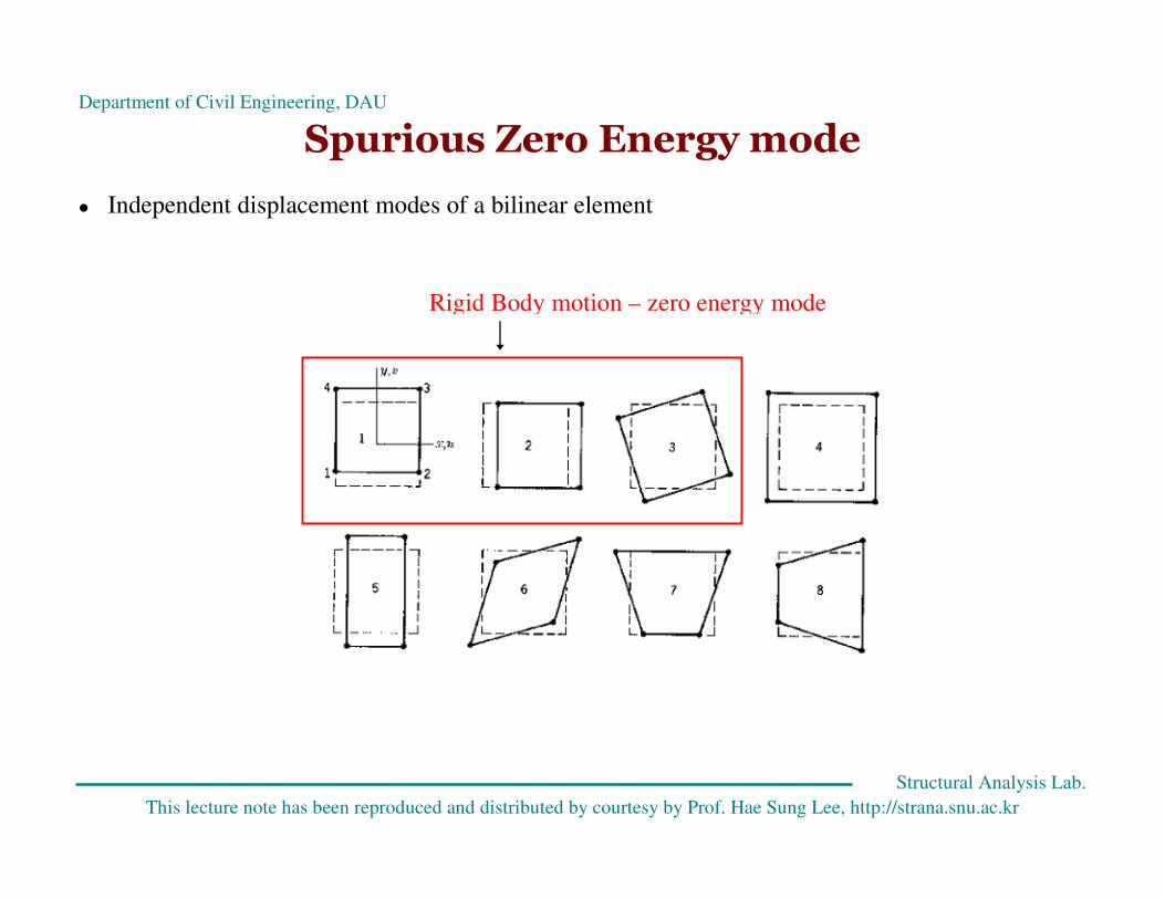
Spurious Zero Energy mode

� Independent displacement modes of a bilinear element

Rigid Body motion – zero energy mode




� Spurious zero energy mode

� Zero energy mode of Q8 element

Hour glass mode




� Zero energy modes of Q9 element

� Near zero energy modes

02 review of mathematicsstrana.donga.ac.kr/lecture/fem/pdf/fem_note.pdf · this lecture note has...

Documents