02 pipe lining summary

8/6/2019 02 Pipe Lining Summary

http://slidepdf.com/reader/full/02-pipe-lining-summary 1/8

Linear Pipelining Techniques

April 14, 2011

This chapter deals with advanced pipelining design in processor development. It dis-cusses how to build

• Instruction Pipelines,

• Arithmetic Pipelines, and

• Memory-Access Pipelines.

The discussion includes

• Instruction Prefetching,

• Internal Data Forwarding,

• Hazard Avoidance,

• Branch Handling, and

• Instruction Issuing.

1 Synchronous Pipeline Model

Synchronous pipelines are shown in Figure 1. Clocked buffers are used to interface be-tween stages. Upon arrival of a clock pulse all buffers transfer data to the next stagesimultaneously. The pipeline stages are combinational logic circuits. It is desired to haveapproximately equal delays in all stages. These delays determine the clock period and thusthe speed of the pipeline.

The utilization pattern of successive stages in a synchronous pipeline is specified by a

reservation table. For a linear pipeline, the utilization follows a diagonal streamline patternas shown in Table 1.This table is essentially a space-time diagram depicting the precedence relationship in

using the pipeline stages.

1



→ Time (clock cycles)

1 2 3 4S 1 XS 2 X

S 3 XS 4 X

Table 1: Reservation table of a four-stage linear pipeline.

1.1 Clocking and Timing Control

The clock cycle τ of a pipeline is determined below. Let τ i be the time delay of the circuitryin stage S i and d the time delay of a buffer as shown in Figure 1, then

τ = maxi

{τ i}k1 + d = τ m + d (1)

The pipeline frequency is defined as

f =1

τ (2)

B u f f e r

Stage

1 B u f f e r

Stage

2 B u f f e r

B u f f e r

Stage

k B u f f e r

Clock

m d

Input Output

Figure 1: A synchronous pipeline model

If one result is expected to come out of the pipeline per cycle, f represents the maximum throughput of the pipeline. However, the actual throughput of the pipeline may be lowerthan f due to branching and load interlocking .

1.2 Speedup, Efficiency, and Throughput

Ideally the total time required for a pipeline to process n tasks is

T k = [k + (n − 1)]τ (3)

2



where τ is the clock period. Consider an equivalent-function nonpipelined processor whichhas a flow-through delay of kτ . The amount of time it takes to execute n tasks on thisnonpipelined processor is T 1 = nkτ .

Speedup Factor The speedup factor of a k-stage pipeline over an equivalent non-

pipelined processor is defined as

S k =T 1T k

=nkτ

kτ + (n − 1)τ =

nk

k + (n − 1)(4)

Optimal Number of Stages Let t be the total time required for a nonpipelinedsequential program of a given function. To execution the same program on a k-stagepipeline with an equal flow-though delay t, one needs a clock period of p = t/k+d, where dis the buffer delay. Thus, the pipeline has a maximum throughtput of f = 1/p = 1/(t/k+d).The total pipeline cost is roughy estimated by c + kh, where c covers the cost of all logicstages and h represents the cost of each latch. A pipeline performance/cost ratio (PCR) is

PCR =

f

c + kh =

1

(t/k + d)(c + kh) (5)

Figure 2: Optimal number of pipeline stages

The peal of the PCR plotted in Figure 2 corresponds to an optimal choice for thenumber of pipeline stages:

k0 =

t · c

d · h(6)

Efficiency and Throughput The efficiency E k of a linear k-stage pipeline is definedas

E k =S kk

=n

k + (n + 1)(7)

3



Obviously, the efficiency approaches 1 when n → ∞, and a lower bound on E k is 1/kwhen n = 1. The pipeline throughput H k is defined as the number of tasks (operations)performed per unit time:

H k = n[k + (n − 1)]τ

= nf k + (n − 1)

(8)

The maximum throughput f occurs when E k → 1 as n → ∞. Note that H k = E k · f =E k/τ = S k/kτ .

2 Instruction Pipeline Design

A typical instruction execution consists of a sequence of operations, including instructionfetch, decode, operand fetch, execute, and write-back phases. These phases are ideal foroverlapped execution on a linear pipeline. Each phase may require one or more clock cycles

to execute, depending on the instruction type and processor/memory architecture used.Fetch stage (F) fetches instructions from a cache memory.Decode stage (D) reveals the instruction function to be performed and identifies theresources needed. Resources include general-purpose registers, buses, and functional units.Issue stage (I) reserves resources. Pipeline control interlocks are maintained at this stage.The operands are also read from registers during this stage.Execution stage (E) is a single or multiple stages reserved for execution.Writeback stage (W) is used to write results into the registers.Note that memory load or store operations are treated as part of execution.

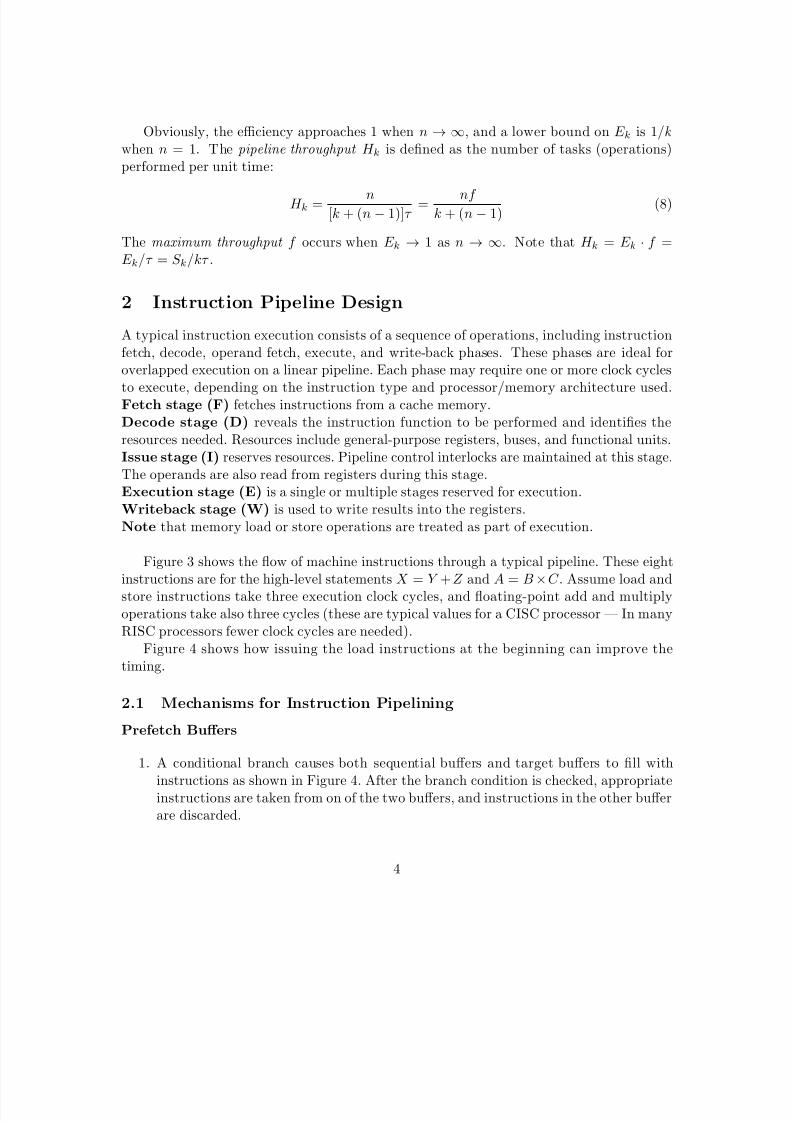
Figure 3 shows the flow of machine instructions through a typical pipeline. These eightinstructions are for the high-level statements X = Y +Z and A = B×C . Assume load andstore instructions take three execution clock cycles, and floating-point add and multiplyoperations take also three cycles (these are typical values for a CISC processor — In manyRISC processors fewer clock cycles are needed).

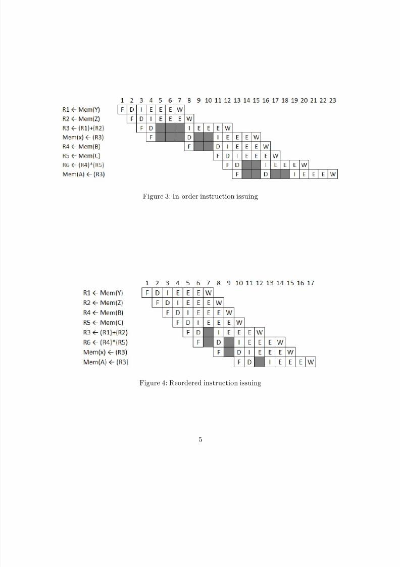
Figure 4 shows how issuing the load instructions at the beginning can improve thetiming.

2.1 Mechanisms for Instruction Pipelining

Prefetch Buffers

1. A conditional branch causes both sequential buffers and target buffers to fill with

instructions as shown in Figure 4. After the branch condition is checked, appropriateinstructions are taken from on of the two buffers, and instructions in the other bufferare discarded.

4



Figure 3: In-order instruction issuing

Figure 4: Reordered instruction issuing

5



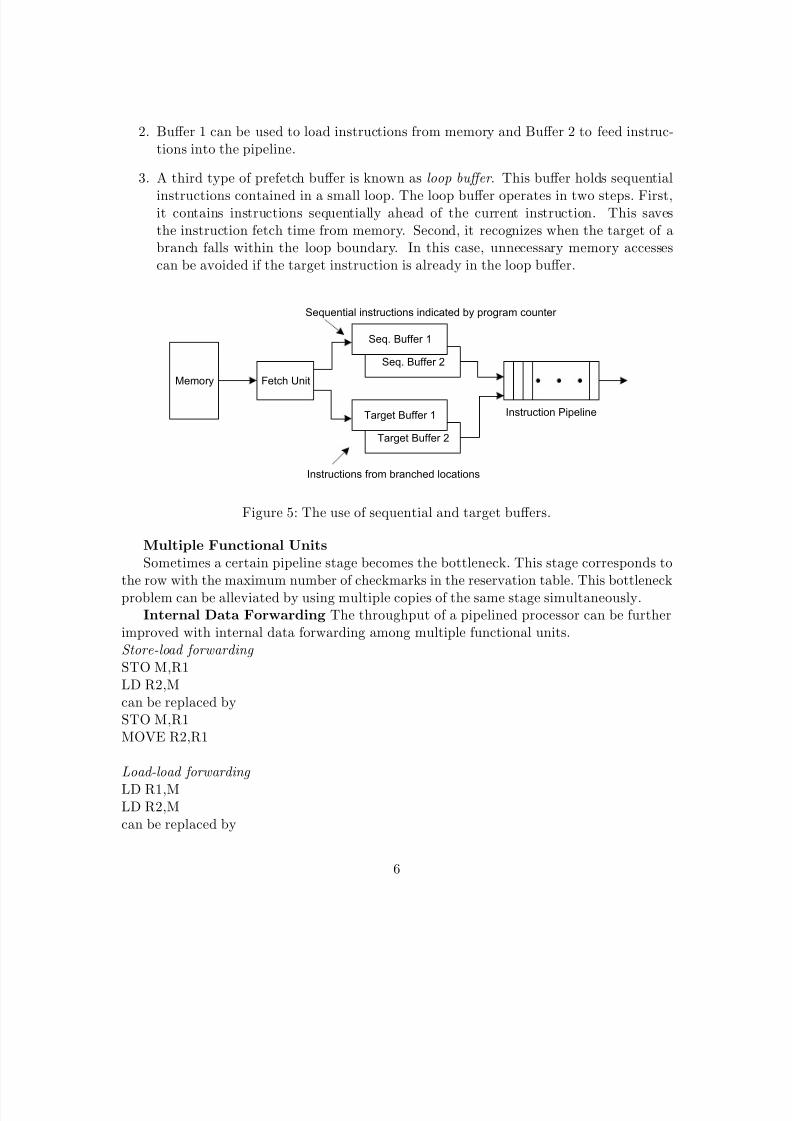
2. Buffer 1 can be used to load instructions from memory and Buffer 2 to feed instruc-tions into the pipeline.

3. A third type of prefetch buffer is known as loop buffer . This buffer holds sequential

instructions contained in a small loop. The loop buffer operates in two steps. First,it contains instructions sequentially ahead of the current instruction. This savesthe instruction fetch time from memory. Second, it recognizes when the target of abranch falls within the loop boundary. In this case, unnecessary memory accessescan be avoided if the target instruction is already in the loop buffer.

Seq. Buffer 2

Memory Fetch Unit

Seq. Buffer 1

Target Buffer 2

Target Buffer 1 Instruction Pipeline

Sequential instructions indicated by program counter

Instructions from branched locations

Figure 5: The use of sequential and target buffers.

Multiple Functional UnitsSometimes a certain pipeline stage becomes the bottleneck. This stage corresponds to

the row with the maximum number of checkmarks in the reservation table. This bottleneckproblem can be alleviated by using multiple copies of the same stage simultaneously.

Internal Data Forwarding The throughput of a pipelined processor can be furtherimproved with internal data forwarding among multiple functional units.Store-load forwarding STO M,R1LD R2,Mcan be replaced bySTO M,R1MOVE R2,R1

Load-load forwarding

LD R1,MLD R2,Mcan be replaced by

6



LD R1,MMOVE R2,R1

Store-Store forwarding

STO M,R1STO M,R2can be replaced bySTO M,R2

Hazard Avoidance The read and write of shared variables by different instruction ina pipeline may lead to different results if these instructions are executed out of order.

Read-after-Write (RAW) hazard Write-after-Read (WAR) hazard Write-after-Write (WAW) hazard

The resolution of hazard conditions can be checked by special hardware while instruc-tions are being loaded into the prefetch buffer. A special tag bit can be used with eachoperand register to indicate safe or hazard-prone. Successive read or write operations areallowed to set or reset the tag bit to avoid hazards.

2.2 Branch Handling Techniques

The action of fetching a nonsequential or remote instruction after a branch instruction iscalled a branch taken . The instruction to be executed after a branch taken is called a branch target . The number of pipeline cycles wasted between a branch taken and its branch targetis called the delay slot , denoted by b. In general, 0 ≤ b ≤ k − 1, where k is the number of pipeline stages. When a branch taken occurs, all the instructions following the branch inthe pipeline become useless and will be drained from the pipeline. This implies losing anumber of useful cycles. Let p be the probability of a conditional branch instruction in atypical instruction stream and q the probability of a successful executed conditional branchinstruction ( a branch taken). Typical values of p = 20% and q = 60% have been observedin some programs. The penalty paid by branching is equal to pqnbτ , hence

T eff = kτ + (n − 1)τ + pqnbτ (9)

H eff =n

T eff =

nf

k + n − 1 + pqnb(10)

When n → ∞, the tightest upper bound on the effective pipeline throughput is

H ∗eff =f

pq(k − 1) + 1(11)

7



We define the performance degradation factor as

D =f − H ∗eff

f (12)

Branch Prediction Branch can be predicted either based on branch code types stat-ically or based on branch history during program execution.

NN NT

TN TT

N

T

T

N

N

T

N

T

T=Branch taken

N=Not-taken branch

NN=Last two branches not taken

NT=Not branch taken and previous taken

TT=Both last two branch taken

TN=Last branch taken and previous not taken

Figure 6: Branch history buffer and a state transition diagram used in dynamic branchprediction.

Delayed BranchesA delayed branch of d cycles allows at most d − 1 useful instructions to be executed

following the branch taken. The execution of these instructions should be independent of the outcome of the branch instruction. Sometimes NOP fillers can be inserted in the delayslot if no useful instructions can be found. However, inserting NOP fillers does not saveany cycles. The delayed branching is effective in short instruction pipelines with aboutfour stages (like in RISC processors).

3 Arithmetic Pipeline Design

Pipelining can be used to speed up numerical arithmetic computations. Depending on thefunction to be implemented, different pipeline stages in an arithmetic unit require differenthardware logic. Since all arithmetic operations (such as add, subtract, multiply, divide,squaring, square rooting, logarithm, etc.) can be implemented with the basic add andshifting operations, the core arithmetic stages require some form of hardware to add orto shift. For example, a typical three-stage floating point adder includes a first stage forexponent comparison and equalization which is implemented with an integer adder andsome shifting logic; a second stage for fraction addition using a high-speed carry lookaheadadder; and a third stage for fraction normalization and exponent readjustment using shifterand another addition logic.

8

02 pipe lining summary

Documents