~) pergamon journal of atmospheric and terrestrial physics, · pdf file~) pergamon journal of...

~ ) Pergamon Journal of Atmospheric and Terrestrial Physics, Vol. 57, No. 4, pp. 333 365, 1995

Elsevier Science Ltd Printed in Great Britain

0021-9169(94)E0013-D

The middle atmospheric response to short and long term solar UV variations: analysis of observations and 2D model results

ERIC L. FLEMING,* SUSHIL CHANDRA,t CHARLES H. JACKMAN,t DAVID B. CONSIDINE* and ANNE R. DOUGLASS]"

*Applied Research Corporation, Landover, MD 20785, U.S.A. ; tCode 916, NASA/Goddard Space Flight Center, Greenbelt, MD 20785, U.S.A.

(Received in final form 18 January 1994 ; accepted 14 February 1994)

Abstract--We have investigated the middle atmospheric response to the 27-day and 11-yr solar UV flux variations at low to middle latitudes using a two-dimensional photochemical model. The model reproduced most features, of the observed 27-day sensitivity and phase lag of the profile ozone response in the upper stratosphere and lower mesosphere, with a maximum sensitivity of +0.51% per 1% change in 205 nm flux. The model also reproduced the observed transition to a negative phase lag above 2 rob, reflecting the increasing importance with height of the solar modulated HOx chemistry on the ozone response above 45 km. The model revealed the general anti-correlation of ozone and solar UV at 65-75 km, and simulated strong UV responses of water vapor and HOx species in the mesosphere. Consistent with previous 1D model studies, the observed upper mesospheric positive ozone response averaged over _ 40 ° was simulated only when the model water vapor concentrations above 75 km were significantly reduced relative to current observations. Including the observed temperature-UV response in the model to account for temperature- chemistry feedback improved the model agreement with observations in the middle mesosphere, but did not improve the overall agreement above 75 km or in the stratosphere for all time periods considered. Consistent with the short photochemical time scales in the upper stratosphere, the model computed ozone UV sensitivity was similar for the 27-day and 11-yr variations in this region. However, unlike the 27-day variation, the model simulation of the 11-yr solar cycle revealed a positive ozone-UV response throughout the mesosphere due to the large depletion of water vapor and reduced HO~-UV sensitivity. A small negative ozone response at 65 75 km was obtained in the 11-yr simulation when temperature--chemistry feedback was included

In agreement with observations, the model computed a low to middle latitude total ozone phase lag of + 3 days and a sensitivity of +0.077% per 1% change in 205 nm flux for the 27-day solar variation, and a total ozone sensitivity of + 0.27% for the 11-yr solar cycle. This factor of 3 sensitivity difference is indicative of the photochemical time constant for ozone in the lower stratosphere which is comparable to the 27-day solar rotation period but is much shorter than the 11-yr solar cycle.

1. INTRODUCTION

In recent years, considerable effort has been made to investigate the middle atmospheric response to variations in solar ultraviolet flux on short and long time scales. The variation in solar UV flux at wavelengths of 120-400 nm affects the stratospheric and mesospheric ozone concentrations through changes in 02 and 03 photodissociation rates, changes in catalytic loss processes such as that due to odd hydrogen chemistry, as well as through induced changes in temperature which affect the temperature dependent reaction rates (GARCIA et al., 1984 ; ALLEN et al., 1984 ; ECKMAN, 1986a,b ; ]HOOD, 1986, 1987 ; KEATING et al., 1987; BRASSEUR et al., 1987; HOOD and DOUGLASS, 1988 ; SUMMERS et aL, 1990 ; CHANDRA, 1991 ; HUANG and BRASSEUR, 1993). Previous studies have also examined the possible indirect solar-induced changes in the large scale circulation and resulting temperature

changes (e.g. HOOD, 1986; HOOD and JIRIKOWIC, 1991). Quantifying the atmospheric response to the 27-day modulat ion in solar UV flux is necessary, for example, to separate it from other naturally occurring phenomena such as the relatively stronger non-solar dynamically-induced perturbations which have similar periods of 3-5 weeks ( C H A N D R A , 1986; HOOD and JIRIKOWIC, 1991). Understanding the response to the 11-yr solar cycle is also important in determining the long term trends induced by anthropogenic influences.

Previous investigations have established many of the fundamentals of the ozone -UV response throughout the middle atmosphere. However, some questions remain, such as a model-data discrepancy above 75 km for the 27-day variation as noted by SUMMERS et al. (1990). Moreover , numerical studies of the 27- day response have involved only 1D models and have viewed the stratosphere and mesosphere separately;

333

334

the 2D model studies of GARClA et al. (1984) and HUAN6 and BRASSEUR (1993) examined the response for the entire middle atmosphere, but only for the 11- yr solar cycle. In this paper, we will address certain details of the 27-day response using a 2D model with pre-specified temperature and circulation fields which do not vary with solar flux. Our goal is to ascertain how much of the observed response can be accounted for by a purely photochemical 2D model. As such, we confine our analysis to the latitudinal region between _+40 ° where photochemistry is most important and where direct solar UV forcing is best detectable. Although our model formulation does not allow for coupling between solar flux and the transport fields (i.e. meridional circulation and eddy diffusion, Kvy, ~-) , we expect such direct solar driven variations to be small, as shown in previous model studies (GARCIA et al. , 1984 ; BRASSEUR e t al. , 1987 ; HUANG and BRASS- EUR, 1993). We will show the effects of temperature- chemistry feedback on the computed ozone response by incorporating into the model a pre-specified temperature response obtained from observations. We will present results for profile ozone for the entire middle atmosphere from ~20 to 85 km, and for total ozone, and compare with observations and previous modeling studies. Using a self-consistently computed water vapor formulation also allows us to show the response of H20 and HOx species to the solar UV. Finally, we will examine the responses of ozone, H:O, and HOx for time scales similar to the 11-yr solar cycle, and discuss how they differ from the 27-day response.

The outline of this paper is as follows. We give an overview of previous observational and theoretical work on the solar UV response in section 2. In section 3 we describe our 2D model and the method of simu- lating the 27-day solar rotation and the 11-yr solar cycle variations in the model. In section 4, we sum- marize the 27-day response of profile ozone seen in the observations, and present our model results and compare with the observations and previous model investigations. Results and comparisons for total ozone are given in section 5, and a summary of the findings and conclusions is made in section 6. The 2D model used in this paper has recently been upgraded to include mesospheric heights (60-90 km), computed water vapor, and improved eddy diffusion par- ameterizations. In Appendix A, we compare model calculations with climatological observations of ozone, water vapor, and carbon monoxide, with an emphasis on the mesosphere. The model horizontal eddy diffusion (K,,~.) formulation is given in Appendix B.

E. L. FLEMING et al.

2. OVERVIEW OF THE OZONE RESPONSE TO SOLAR UV

Over a 27-day solar rotation, the observed amplitude of the UV variation is reported to be 20% near 120 nm, 3% at 200 nm, and < 1% at 300 nm (LEAN, 1987; SUMMERS e t al. , 1990). Analogous quantities over the 11-yr solar cycle are not as well observed, and questions still remain as to the long term spectral variations in UV. For the 27-day variation, HOOD (1986, 1987) and KEATI~G et al. (1987) observed a positive correlation between ozone and 205 nm flux at 30-60 km in the tropics using Nimbus-7 SBUV, LIMS, and SAMS d~ata. Qualitatively, the positive response is caused by the increased production of odd oxygen via photodissociation of O2 by solar flux near 200 nm. The response maximizes near 2-3 mb with a sensitivity of 0.5% per 1% 205 nm solar flux change. GARCIA et al. (1984) and HUANG and BRASSEUR (1993) computed somewhat smaller stratospheric responses in their 2D model studies of the 1 l-yr solar cycle. The HOOD and KEATING e t al. studies observed a 27-day response phase lag of about +5 days near 10 mb which decreased to near zero at 2-3 mb, and reversed sign above 2 mb (ozone leading UV) which they attributed to temperature feedback effects. Similar findings were made by BRASSEUR et al. (1987) in their 1D model study. Previous model studies have calculated a direct solar-induced temperature response of 0.5-2 K below 75 km (GARCIA et al. , 1984; BRASSEUR et al. , 1987; SUMMERS et al. , 1990; HUANG and BRASSEUR, 1993), with small associated changes in circulation and eddy diffusion. Observational studies indicate a temperature-UV response of 0.5-1.5 K in the middle atmosphere (HOOD, 1986 ; KEATING et al. , 1987 ; HOOD and JIRIKOWIC, 1991), along with the possibility of an indirect solar-induced dynamical component of the temperature response which may explain the fact that the observed upper stratospheric temperature-UV phase lag of 6-10 days is significantly larger than predicted by photochemical-radiative models (BRASS- EUR e t al. , 1987).

Because the ozone-UV response decreases rapidly below 35 kin, the response of total ozone is small and difficult to infer from observations. Theoretical model calculated changes in column ozone range from 0.3 to 4.0% for solar UV changes over the course of a solar cycle (e.g. GARCIA et al. , 1984; BRASSEUR et al. , 1987; HUANG and BRASSEUR, 1993). A similar total ozone response to solar cycle variations was inferred from Nimbus-4 and Nimbus-7 satellite data, and from the ground based Dobson station network (CHANDRA, 1984; REINSEL e t al. , 1987, 1988; CHANDRA, 1991; HERMAN e t al. , 1991). CHANDRA (1991) also found that for the UV variations over a 27-day solar

Middle atmosphere response to solar variations 335

rotation, total ozone lagged the solar UV by 3-4 days, and that the sensitivity of + 0.11% (per 1% change in solar UV at 205 nm) was a factor of 2-3 less than that for a solar cycle. This difference was attributed to the photochemical time constant of ozone in the lower stratosphere, which is comparable to the 27-day solar rotation period but is much shorter than the 1 l- yr solar cycle period.

The ozone-UV :response in the mesosphere was examined by KEATmG et al. (1987) and HOOD et al. (1991) using data from the Solar Mesosphere Explorer (SME). They obtained a negative ozone-UV correlation at 63-78 km, with a positive response above and below this layer for the 27-day solar rotation. The negative response in the middle mesosphere is thought to be caused by lhe increased Lyman alpha dis- sociation of H20 and subsequent increase in concentrations of odd hydrogen species (HOx = H, OH, HO2) which catalytically destroy ozone. The model results of GARCIA et al. (1984) and HtJANG and BRASS- Et;R (1993) for the 11-yr solar cycle were in general agreement with these observations. In their 1D model study of the 27-day variation, SUMMERS et al. (1990) also reproduced these observations below 75 km. However, they simulated the positive response in the upper mesosphere only by significantly reducing the model water vapor below current ground based microwave observations (BEVILACQUA et al., 1989). Previous model calculations have also been unable to reproduce the large positive temperature response near 70 km observed by KEATING et al. (1987).

3. 2D MODEL DESCRIPTION

For this study, we used our two-dimensional (2D) photochemical model with pre-specified temperature and transport fields which extends from the ground to approximately 9,0 km (0.0024 mb) and has a vertical grid equally spaced in log-pressure with a reso- lution of ~ 2 km (DOUGLASS et al., 1989; JACKMAN et al., 1990). The latitudinal extent is from 85°S to 85°N with a 10 ° grid spacing. The climatological temperature field is based on National Meteorological Center (NMC) data for the ground to 0.4 mb, and CIRA (1972) for levels above 0.4 mb. Heating rates and the residual circulation were calculated following ROSENFIELD et al. (1987), using SME ozone data for the mesosphere.

There are 23 tran~,;ported species or families, including Ox (03, O, O(~D)), NOz (N, NO, NO2, NO3, HOENO2, N205, and C1ONO2), Cly (C1, C10, HOCI, HC1, and C1ONO2), Bry (Br, BrO, HBr, BrONO2), HNO3, H20, N20, CH4, H2, CO, CHaOOH, CFCI3,

CF2C12, CHsC1, CC14, CHC1F2, C2C13F3, C2C12F4, C2CIF5, CH3CC13, CBrC1F2, CBrF3, and CH3Br. Reaction rates and photodissociation cross sections were taken from DEMORE et al. (1990). The upper boundary conditions are zero flux for all species. The lower boundary condition for ozone is a deposition velocity of 0.1 cm s ~. Lower boundary conditions for the other transported species are based on 1990 values (WMO, 1990) and are given in Table 1. Lower boundary conditions for HNO3 and NO= were determined as follows. We used the tropospheric chemistry model results of THOMPSON et al. (1990) to calculate the total concentration of NOy (NOz+HNO3) at the lower boundary at a given latitude as a function of marine or continental conditions. We then weighted these values by the percentage area of land or ocean at each latitude, as given in SELLERS (1965), to produce a zonal mean NOy boundary condition for each model latitude. These were then used to determine the lower boundary conditions for HNO3 and NO= for each latitude, using a partitioning ratio of 30% for HNO3 and 70% for NO=. This ratio was based on aircraft measurements of ATLAS et al. (1992). Based on these computations and the THOMPSON et al. (1990) model results described above, we obtained area weighted global average lower boundary conditions of 45 pptv for HNO 3 and 105 pptv for NOz.

To properly simulate the HOx chemistry in the mesosphere, we incorporated computed water vapor in the 2D model. All photolytic and chemical production and loss processes of H20 were included, and tropospheric water vapor below 400 mb has been fixed to the climatological values of OORT (1983). Water vapor loss due to rainout in the upper troposphere above 400 mb is computed in a split process. That is, the chemical production and loss, as well as transport and diffusion were first used to compute an "intermediate updated" value of water vapor. All "intermediate" water above 50% relative humidity was then rained out separately to give a final updated water vapor concentration. This methodology is similar to that used in STORDAL et al. (1985). Our tropospheric water vapor, along with the NOz and HNO 3 boundary condition described above, produced a methyl chloro- form (CH3CC13) lifetime of 6.3 yr, within the range of observed values (WMO, 1992). Our tropospheric OH/HO2 ratios are also in agreement with those of the one-dimensional photochemical model results of the troposphere (THOMPSON and STEWART, 1991; THOMPSON et al., 1993). More detailed comparisons of our computed ozone and water vapor fields with observations throughout the model domain are given in Appendix A.

The horizontal eddy diffusion (gyy) formulation is

336 E.L. FLEMING et al.

Table 1. Lower boundary conditions for all transported species in model simulations for the year 1990 (WMO, 1990)

Type of boundary Species condition (units) Value

N20 Mixing ratio (ppbv) 310 CH4 Mixing ratio (ppmv) 1.675 CO Mixing ratio (ppbv) 100 H2 Mixing ratio (ppbv) 500 CH3OOH Flux (cm -2 s-l) 0.0 CH3C1 Mixing ratio (pptv) 600 CH3CCI 3 Mixing ratio (pptv) 150 CC14 Mixing ratio (pptv) 105 CFCI3 Mixing ratio (pptv) 275 CF2C12 Mixing ratio (pptv) 468 C2C13F 3 Mixing ratio (pptv) 51 C2C12F 4 Mixing ratio (pptv) 7 C2C1F5 Mixing ratio (pptv) 5 CHCIF2 Mixing ratio (pptv) 111 04 Deposition velocity (cm s-t) 0.1 HNO 3 Mixing ratio (pptv) 45 NOz(wo HNO3) Mixing ratio (pptv) 105 CI~ Flux (cm -2 s 1) 0.0 CH3Br Mixing ratio (pptv) 10 CBrF3 Mixing ratio (pptv) 3.2 CBrC1F2 Mixing ratio (pptv) 1.8 Brx Flux (cm -2 s i) 0.0

Units are in parts per million by volume (ppmv), parts per billion by volume (ppbv), and parts per trillion by volume (pptv).

described in Appendix B ; a latitude-height cross section of the model K,. for December is shown in Fig. B-1. The vertical eddy diffusion (Kz~) is prescribed as follows: in the troposphere, Kzz is a function of latitude; the largest values occur in the tropics with a monotonic decrease towards the poles. In the stratosphere, Kzz is independent of latitude and was determined to provide a computed water vapor field which reasonably simulates Nimbus-7 LIMS observations (see Figs A-7 to A-11). In the mesosphere, we adapted a Kzz profile which increased by a factor of 3 from 50- 90 km, fixing the top model level to the maximum K~z value possible in the mesosphere (6× 10 4 c m 2 s -1)

for a time step of one day, without inducing numerical instability. This profile has a height variation similar to that used by STROBEL et al. (1987) who derived their K= profile based on providing a best fit of their model computed water vapor with ground based microwave H~O measurements. Our resulting K= profiles are shown in Fig. B-2. Note that K~ is independent of season and varies with latitude only in the troposphere.

To simulate the 27-day solar rotation variation, a sine wave with a 27-day period and a pre-specified amplitude modulation for a given wavelength interval was incorporated into the 2D model. The amplitude modulation (the ratio of the perturbed to baseline

solar flux) varies with wavelength from 10% at Lyman alpha (121.6 nm), to 1.5% at 200 nm, and <0.5% at 300 nm, as taken from SUMMERS et al. (1990), and corresponds approximately to those observed during the SME time period. The model was then run with the photolysis calculations updated every day to obtain a time dependent simulation for the 27-day response. To simulate the response over an 11-yr solar cycle, we ran steady state simulations with the solar flux held constant throughout the model run using: (1) the baseline solar flux, and (2) the perturbed solar flux corresponding to twice the amplitude modulations described above. Our model calculations revealed that the response was essentially linear, that is, the species change per 1% change in UV was independent of the magnitude of the solar flux perturbation. As such, we present computed species changes which have been normalized to the solar flux change. Since we are studying the photochemically driven aspects of the response, we confine our analysis on an annually averaged basis to low and mid-latitudes where the meridional transport effects on the computed response are expected to be small. As such, we do not consider high latitude stratospheric ozone changes such as that which may be induced over a solar cycle by ther- mospheric NOx production. All model simulations were run for 20 yr to obtain a repeating seasonal cycle.


We used the final year of model output to compute correlation coefficients and sensitivity factors between 205 nm flux and ozone mixing ratio at each altitude, and for total ozone, as a function of phase lag. Note finally that we do not include results above 85 km since the model simulations above this level are strongly influenced by the top boundary condition ( ~ 90 kin).

4. RESULTS--PR()FILE OZONE SOLAR RESPONSE

4. I. Observations

To review the observed 27-day solar variation response, we computed the correlation coefficients and sensitivity factors (% change in ozone per 1% change in 205 nm flux) as functions of altitude from time series of daily ozone and solar UV flux for time lags from - 3 0 to +30 days. Mesospheric (0.75- 0.0056 rob, ~50-85; km) ozone mixing ratio values from the SME IR instrument for the period 1982- 1983 were used which, although in the declining phase of the solar cycle, were still influenced by a [elatively high level of solar activity. We used stratospheric (30- 1 mb) ozone mixing ratio data from Nimbus-7 SBUV for 1 9 8 2 - 1 9 8 3 corre:~ponding to the SME time period. For corresponding solar flux values, the R(MGIIc/w) index was used whic:h has spectral characteristics similar to solar UV at 205 nm. This index (referred to as MgII) is based on the core to wing ratio of the magnesium h and k lines measured from the SBUV spectrometers on Nimbus-7 and the SBUV/2 spectrometer on NOAA.-9 in their continuous scan modes (HEATH and SCHLESINGER, 1986; DONNELLY, 1991; DELAND and CEBULA, 1993).

For the initial analysis, the ozone time series were latitudinally averaged over 40°S-40°N to minimize dynamical signals which have near equal but opposite low latitude perturbations in the two hemispheres. We will discuss the latitudinal variations of the response later in the paper. All time series were smoothed with a 5-day running mean and then deseasonalized by subtracting out the 35-day running mean. The resulting correlation coeff~cients are presented as a function of phase lag and altitude in the contour plot in Fig. 1 (adapted from CHANDRA et al., 1993), and are consistent with previous analyses (HOOD, 1986, 1987; HOOD et al., 1991 ; KEATING et al., 1987). A dominant 27-day response is seen at all levels. Ozone and solar UV are positively correlated throughout the stratosphere and lower mesosphere up to ~ 60 km and in the upper mesosphere above 75 km, and negatively correlated in the middle mesosphere between 60- 75 km. The maximum ~orrelation in the stratosphere

occurs at 40-45 km (+0.57) with a sensitivity factor of +0.46%+0.016 and phase lag of 0 to - 2 days (see Fig. 6a-b for vertical profiles of the maximum sensitivity factors and phase lags). Below 10 mb, the phase lag increases with decreasing height to + 10-12 days at 30 mb, due to the increasing photochemical time constant of ozone. The corresponding correlation and sensitivity decrease below 10 mb to relatively small values at 30 mb.

The observations reveal that the phase lag becomes increasingly negative with height above 2-3 mb (ozone leads UV). Previous studies have attributed this to being a result of the positive temperature response being in near-quadrature with the solar UV perturbation which in turn produces a negative ozone response through the strongly temperature dependent Chapman chemistry (HOOD, 1986, 1987; KEATING et al., 1987 ; BRASSEUR et al., 1987). We will discuss the significance of this phase change later in the context of our 2D model simulations.

In the mesosphere above ~ 60 kin, solar-modulated odd hydrogen concentrations induce a negative solar UV ozone response which maximizes near 70 km where solar absorption reaches unit optical depth. Figure 1 shows a peak correlation at 70 km of -0 .55 , and a sensitivity to MglI (205 nm) of - 1.15% ___ 0.065, with a phase lag of -13 .5 days (180 ° for a 27 day period) (Fig. 6a-b). The response becomes positive above 75 km, as H20 and HOx concentrations are diminished, and the solar-induced odd oxygen production plays the dominant role in determining the ozone distribution. The positive response peaks near 80 km (correlation = +0.22; sensitivity = +0.64% _ 0.10) with the phase lag decreasing from + 5 days at 76 km to - 1 . 5 days near 85 km (Fig. 6a-b) (in general, the ozone sensitivity to solar Lyman alpha UV is a factor of 4-5 smaller than that for the 205 nm (MglI) flux--see KEATING et al., 1987; HOOD et al., 1991).

4.2. Model simulations

Analogous to Fig. 1, the model results for the 27- day solar variation are shown in the correlation contour plot in Fig. 2. Note that the model results are generally smoother and have a higher degree of correlation, compared to observations, due to the lack of natural background variability and instrumental noise, and the smooth sinusoidal solar UV forcing function that we have incorporated. The simulation in the stratosphere and lower mesosphere below 80 km is in good agreement with the observations and previous theoretical work. Maximum positive ozone- 205 nm correlations of greater than 0.9 are seen every-

338 E. L. FLEMING et al.

0.001

0.010

~" 0.100

1 . 0 0 0

10.000

I I I I

' , . ~ _ ~ - - 2~Oo~, O . ~ o ~ - . ' - _ _ _ ' % 0 \ "",~°'~°.,'h\ ,~."" ~ ," " ~ ) 2~

~ '.L\'\ '\ '-. ~\\\'~69o ~-- ,, '~ , ~ . ~ ~L~(,~: C

~o::-, "_-_~"~ r-~-2"-2-"<2~'-~. `, : . . . ~ . ~ L _ ~ o -

-~l i , ~ . . , ,, ~, , , o~ i i i o / / \ I I I I ~ k k I - -

~, ,,,,~o. , , , , . . . . . . R,.o \ \ \ \ \ \ \ \ \ \ \ \ \

O u , - " ~ z ~ . ~ ' , ~ - ~ ' ~ 0 ~ \ ~ ~ ~*O^ ' . Z-_-- TM \ "0. (4, \ ~ - ~ % ~.; I "uO. " - _ o - -

t 95

90

85

80

75

70 ~ ,

6o~

50 ~

~ s ~

40 <

35

30

25

- 2 0

1 0 0 . 0 0 0 I I I I I 1 5

- 3 0 - 2 0 - 10 0 10 20 30 PHASE LAG (DAYS)

Fig. l. Ozone-solar UV flux correlation coefficient as a function of phase lag and altitude derived from Nimbus-7 SBUV (30-1 mb) and SME IR (0.75~).0056 mb) ozone data for 1982-1983, deseasonalized and averaged over 40°S-40°N as discussed in the text. The MgII index (described in the text), which corresponds

to wavelengths near 205 nm, was used (adapted from CnANDI~A et al., 1993).

0.001 I I I I I 95

- 9 0

.~ ~. ~ . • , , _, ,,o,. • .? ~,'.o; ,-_--~-~ 85

g x \~,xx ~--'x'~x s r x \ xx k \x\x ~ ~ x

/ %~ ,%>, K" J .%~,,~

._.~' o.1oo .. ..,,,,,,, ,.'-'"~-----.- "-.., . . . . "",', ,. ~ ' ~ ~ ,o ~'"

\ \ \\\\\%Y~\\~\i\i\\\\~,e so < !} 'C' :&llllll Ig ~ \ \ \ \ \ \ \ I\\\\\\\\~'"' e ,",,% x r,- 1 . 0 0 0 ; h~wcn~ ~ ~ ~ ~'~ 4 5 O

" ~ i i ~ / / / / / ' '"' ..... """'" '" / / ~ ' " ~ . I ~ H b~ ''~ " " ' "" "- "',',, ','" ',"i ~o~ ,,. ,, .......... ,. ~,,,,,.,,~ ~ ~ , , ' T ~ , \ \ \ \ \\\N'~ . . . . ' " ~

~ . _ _ _ _ _ . ~ , , ~ \ ~ , ~ .....---- . . . . ~ ~ ,'_T~'o ~_-" _' ,., N . \ ~ - - j I , b'.~.~ - . , ,' ' " 2

I O0.OOC -- I ,,., ~ " " < - - , - ' / - - / - " 15

- 3 0 - 2 0 - 1 0 0 10 20 30 PHASE LAG (DAYS)

Fig. 2. Ozone-205 nm solar flux correlation coefficient as a function o f phase lag and altitude derived from model calculations of the 27-day solar variation. All time series have been deseasonalized and averaged

over _+ 35 °.


where between 30 and 65 km, with the response falling off rapidly with decreasing height below 30 km (10 mb). Above 10 mb, the phase lag decreases with increasing height fi'om a value of + 5 days at l0 mb to near zero days at 2-3 mb. The maximum sensitivity (+0.51%) also occurs at 2-3mb, consistent with observations. The phase lag becomes increasingly negative with height in the lower mesosphere, with a value of - 2 . 5 days near 60 km. Since the model uses a pre-specified climatological temperature field which does not vary with solar flux (no temperature chemistry feedback), we attribute the change-over to a negative phase lag above 40 km to the increasing influence with height of HOx chemistry on the solar- modulated ozone concentrations, offsetting the solar- induced odd oxygen increase. This result is at variance with the 1D model simulations of BRASSEUR et al.

(1987) who obtained a negative ozone-UV phase lag above 40 km only when the feedback between ozone and temperature was included.

In the middle mesosphere, the solar-modulated HOx concentrations induce a negative ozone-solar flux correlation. The phase lag of the maximum negative response is near zero as seen in the observations, and the peak negative correlation ( -0 .85) and sensitivity ( - 0 . 9 5 % ) occur at 75-80km, which are slightly higher in altitude than observations (70-72 km). These results below 80 km are also qualitatively similar to the theoretical work of SUMMERS et aL (1990).

The associated solar responses of H20 and HO~ (H + OH + HOE) are shown in Figs 3 and 4, again as functions of phase lag and altitude. Here we present the sensitivity factor (per cent change per 1% change in solar flux) of these constituents to Lyman alpha flux, since mesospheric H20 and HOx have the stron- gest response to radiation at this wavelength. As expected, water vapor reveals a large negative response above 65 km with a maximum sensitivity of - 0 . 4 4 % at the top model level ( ~ 85 km). The phase lag is + 6 (or -7 .5 ) days, consistent with the photochemical lifetime of mesospheric water vapor (BRASSEUR and SOLOMON, 1984). This also implies a phase lag of near 9(I ° for a 27-day period, which is the maximum lag for a direct response to sinusoidal solar forcing based on a linear perturbation analysis of the constituent continuity equation (HOOD, 1986 ; BRASS- EUR et al., 1987 ; CI~EANDRA, 1991). The corresponding HOx response (Fig. 4) is positive throughout the upper stratosphere and mesosphere with the largest value (+0.39%) again at the top model level. The magnitude of the mesospheric HO~ sensitivity reflects that of water vapor, since HOx production at these levels is directly related to the photodissociation of water. The phase of the 1-IO~ response is - 1 to - 2 days

above 65 km ; this is a mid-range value between the water vapor response (phase of - 7 . 5 (or +6) days) and the solar forcing itself (zero phase lag), both of which control the solar modulated HOx production in the mesosphere. HOx exhibits a relatively weak solar response in the stratosphere which changes sign at 10mb. The negative H O < U V correlation below l0 mb is probably due to a combination of effects due to the solar modulation of odcl oxygen [03, O, O(~D)] production, and changes in the HO~ family partitioning which may increase or decrease the actual odd hydrogen concentrations. A detailed analysis of this is beyond the scope of the present paper.

The model simulated ozone response in Fig. 2 does not reveal the observed positive correlation above 75 km (Fig. 1)--a fact most likely related to the local water vapor concentrations (this is probably not an artifact of the non-solar varying temperature field used in the model as will be discussed later). SUMMERS et al. (1990) found that a net increase in HOx catalytic ozone loss due to enhanced solar flux occurred above 80 km when the water vapor abundance reached a certain threshold level, estimated to be 1.5 ppmv at 80 km. The water vapor time scales for photochemistry and replenishment via upward transport are both ~ l0 days in the upper mesosphere. Therefore, a negative ozone-UV response could persist in the upper mesosphere over the course of a 27-day cycle, if the local water vapor amounts were large enough. By reducing the model mesospheric water vapor amounts (via reduction in eddy diffusion by a factor of five), SUMMERS et al. obtained a positive ozone-UV response above 75 km peaking near 80 km, similar to observations. The water concentrations were reduced by a factor of four at 80 km and by more than a factor of 25 at 90 kin. To simulate the observational response above 75 km in our 2D model, it was necessary to reduce the water vapor concentrations by a factor of 1.5 at 70 km, 15 at 80 km, and 25 at 90 km using a methodology similar to that of SUMMERS et aL described above. The resulting ozone-205 nm correlation plot is shown in Fig. 5, and is similar at all levels to the observations in Fig. 1. The response is qualitatively similar to the standard H20 response (Fig. 2) below 78 km, although the level of maximum negative response has decreased in altitude from ~ 77 to 73 km and is closer to that seen in observations. Also, the magnitude of the negative correlation at 65- 78 km has been reduced due to the lower water vapor amounts. Above 78 km, the response in Fig. 5 is positive as less water vapor is available for generation of HOx by the increased UV, and the ozone response is controlled by the odd oxygen increase. Our goal here was to estimate the magnitude of the water vapor


0.001 I ~ I I ) 95

90

O.OlO ',~---" ,1t ,? ~ - - - ? / ~ ' , - ~ _ _ . " Z~"-,,,'--.-.-.-~/~ °" ,.'. _ - . " ~ :~L\\~ ~ l l l ~ o . , . . , " ,,,E\\~ ~ 1 1 ~ " 75

'~- . . . . : ' i ' , ~ / V . . . . , ' , ,~\ '-~-v)~ .o~ "-~-Z-'.- "-Z-Z-" v

o.1oo

:. - s s

03 Z i " 0 0 SO x <

~_~ 1.ooo - ~ ~ - o . o o o ~ _ 14~ o ~Ooo .Ooo ~ °.ooo k." 40

,o0oo A L :: <_ o.oo.ooo

- 3 0 - 2 0 - 1 0 0 10 20 30 PHASE LAG (DAYS)

Fig. 3. Sensitivity (% change per 1% change in solar flux) of water vapor to Lyman alpha (121.6 nm) radiation as a function of phase lag and altitude derived from model calculations of the 27-day solar

variation. All time series have been deseasonalized and averaged over + 35 °.

0.001 ~ I I t I 95

- 90

0 . 0 1 0 " • - , ,~ , J , ~ \ ' o ' N , , ~,~-~ ~ .~ ' /~ ~o

' , ' , ' .__,' ,~,._,'II 70

= o . 1 o o l~ , , . . . .~ i~ i \ \ / , " " , ~\\~,~o

, , , ' ! i l l \ \ 7 ' , ' , so ~ ~ 5 ,,,o 1 , , , ))%~.--",:11%/ ' ~ ' - - - " , ' , / " o o ~ , , 0 ~°

_ . J -._o.o,o,D ~.o,;_J , ,-o.o,o--L>~.o,°_; ~ ~ - - < - ~ ~ - - ° . , ~-~,~o lOoOO0

,!) ,'I> II ,2` o ~' , ~' •

1 0 0 . 0 0 0 I-" o' ~I -0P~" /I ~ "i ,.o'~ I ,~9" { ,: 20 15 - 3 0 - 2 0 - 1 0 0 10 20 30

PHASE LAG (DAYS)

Fig. 4. As in Fig. 3, but forthesensit ivity o f H O x ( H + O H + H O 2 ) to Lyman alpha.

r educ t ion necessary to resolve the obse rved u p p e r mesosphe r i c posi t ive r e sponse in ou r 2D m o d e l s imu- lat ions. How e ve r , as SUMMERS et al. (1990) no te , it is n o t likely tha t the actual wa te r v a p o r a m o u n t s are

as m u c h as an o r d e r o f m a g n i t u d e lower t h a n the obse rva t ions suggest , a n d tha t the deficiency m a y p o i n t to some o the r p rocess wh ich is n o t a c c o u n t e d for in p re sen t m o d e l fo rmula t ions .

Middle atmosphere response to solar variations

n.,

0.001

0.010

0.100

1.000

10.000

100.000

- 3 0

I I

~\V~ " - f ~ o ~ ;.

' I t ! I " x ,~\~, I~1 • ~ t l l l l l I % i%t l t

1;;I I i I I ~ I i i I t I v I I ,A\ttttt , .,,,

. , , ,#,, , ' , , t! o, ~-~ \\~\~;,,'~,,,;,,, ~:

-20 -I(

I I I

I ¢~ I I / ,

"11111 ' / -- \ \ •

' ~ ~ . ~ . ' . ' : , ~ \ \ \ \ \ \ \ " V

t < i l l :ll l l l l l l I% I i i i i l l l l I I I I I?1 i I I i i i l l l l l { ) r,, bill I i l I L ' I ' I I %1il I I b

~ z 2 )rg", \ ~ )

/ / ,.5~_7./(e..<..___j ~ . _ ~ _ - , O

45

40

35

30

25

20 15

10 20 50

95 90

85

80

75

70 ~"

65 --~

80 ~ I - -

55 ~,

50 X

PHASE IAG (DAYS)

Fig. 5. Ozone-205 nm solar flux correlation coefficient as in Fig. 2, but from model calculations using water vapor which has been reduced above 60 km as discussed in the text.

341

The results presented above are summarized in Fig. 6(a) and (b) which show vertical profiles of the maximum sensitivity factors and phase lags of the ozone-UV response obtained from observations and from the two model scenarios using standard and reduced H20 presented above (results from a third model scenario shown here are described below). The observations are based on SME and Nimbus-7 SBUV ozone and the MglI UV index for the 1982-1983 period used in Fig. 1. Figure 6(a) and (b) also shows the stratospheric ozone-UV response during solar maximum of solar cycles 21 and 22 based on Nimbus- 7 SBUV for the 1979-1981 period and the recently reprocessed NOAA-11 SBUV/2 data for the 1989- 1990 period (PLANET et al., 1993). Below 60 km, the model simulations with standard and reduced H20 are nearly identical and reproduce the general features of the observed response, including the maximum sensitivity at 40-45 kra and the change-over to a negative phase lag above 45 km. The simulation above 75 km is greatly improved with the reduced water vapor computation, which gives a positive response at these levels. Also note that the peak negative response at 70-75 km is significantly lower in altitude in the reduced water sin~tulation and is thus closer to that seen in the observations (Fig. 6(a)), although the agreement in the magnitude of the maximum negative response is not as good as in the normal water case.

As discussed earlier, previous studies have examined the impact of temperature-chemistry feedback on the ozone-UV response. To investigate this in our model calculations, we incorporated the observed solar-induced temperature response into the model by means of a sine wave with a 27-day period as was done for the solar UV perturbation (standard H 2 0

was used). We adapted amplitude and phase values as a function of altitude from the analyses of HOOD (1986) and KEATING et al. (1987) for the stratosphere, and HOOD el aL (1991) for the mesosphere. Peak amplitude values occur near 48 km (+ 0.06% (0.16 K) per 1% 205 nm change) and 68 km (+0.14%, 0.3 K), with the phase decreasing from + 8 days at 40 km to near 0 days at 70 km (note that this temperature response created only small changes in the transport fields). The results are shown in Fig. 6(a) and (b) (the third model scenario) and reveal that the computed ozone response at 40450 km is 1-2 days more negative in the phase lag, and the sensitivity is slightly larger, relative to the model run with no temperature response. These changes are consistent with the temperature perturbation at these heights being approximately in quadrature with the UV. This slightly enhances the ozone response through the negative ozone/temperature feedback from Chapman and HOx chemistry (the latter being weakly temperature dependent), and increases the negative time lag between ozone and solar flux (BRASSEUR et al., 1987 ; KEATING


(a)

v

h i P~

( / )

Ld ne 13.

0.001

0.010

0.100

1.000

10.000

A

[]

X

100.000

- 2 . 0

r i i I

// ./ )~

i ~.~

• SME 1982-83 i x ~" ;~

zXNlmbus-7 SBUV 1979-81 !i X ~,t rA i

[3 N imbus-7 SBUV 1982-83 : ~-~z: i ~ . ~ . ~ ' '

XNOAA-11 SBUV/2 1989-90 : . -~ ' . . i .~ ' "

Model - Reduced H20 i~i~'

Model - Standard H20

....... Model - Standard H20 w/ ter~p feedback i I I I I

- 1 . 5 - 1 . 0 -0.5 0.0 0.5

OZONE-205 nm SENSITIVITY (%0 CHANGE)

95 - 9 0

- 85

- 8 0

- 7 5

- 7 0 ~

- 6 5 ~ "

60 ~ k -

55 ~,

50 < X

,,5 o I1 .

40 " <

35

30

25

20 15

.0

(b) 0.001

0.010

0.100

w

1.000

10.000

Z~

[]

X

I I I I I I

• SME 1982-83 " ' ~ i ~

XNOAA-11 SBUV/2 1989-90 L ~ ,

Model - Reduced H20 ~ " ~ "

- - Model - Standard H20

i 95 90

85

80

75

70 :~ 3¢:

65~" 60 ~

I---

55 ~,

50 < X

45 ~ a _

40 a. <

35

30

[] zx 25

20 I 15

8 12

. . . . . . . Model - Standard H20 w / femb feedback 1 0 0 . 0 0 0 I I I I / - I I

- 2 4 - 2 0 - 1 6 - 1 2 - 8 - 4 0 4 OZONE-205 nm PHASE LAG (DAYS)

Fig. 6. Vertical profiles of the ozone-205 nm flux (a) sensitivity, and (b) phase lag derived from : observations for the different time periods indicated ; and from the model calculations using reduced H20, and

using standard H20 with and without temperature-chemistry feedback.

et al. , 1987). However, incorporating the observed temperature response has not necessarily improved the overall model comparison with the stratospheric observations in terms of phase lag, and has slightly worsened the comparison in sensitivity, for the three

time periods shown. At 65-75 km, the temperature response is nearly in phase with the UV so that the negative ozone response is enhanced when the temperature response is included and is cioser to the SME observations. Only a small (if any) phase difference


would then be expected in the middle mesosphere by including temperature feedback, as is illustrated in Fig. 6(b). In the upper mesosphere, the observed temperature response i:s small (0.03-0.05% per 1% change at 205 nm) with a phase near - 2 days, so that including temperature feedback with standard water in the model only slightly enhances the negative response (it does not produce the observed positive response).

We have presented this temperature feedback scenario to illustrate the effects of incorporating a par- ticular observed temperature response on the model calculations. As was shown here and in previous investigations, accounting for the observed temperature- chemistry feedback in this manner requires proper determination of the temperature response phase lag. It is important, therefore, to recognize the possible uncertainties inherent in such an analysis. Previous theoretical studies have predicted only small direct solar-induced temperature fluctuations on the 27-day and 11-yr time scales (maximum of 1-2 K below 75 km), along with small associated changes in zonal wind (0.5-3 m s-i),, meridional circulation, and horizontal and vertical eddy diffusion coefficients (1-3%) (GARCIA et al., 1984; BRASSEUR et al., 1987; HUANG and BRASSEUR, 1993). Therefore, one must be careful when separating the direct and indirect solar induced oscillations from tlae stronger dynamical (non-solar) fluctuations which have periods near 27 days.

Note that the stratospheric observations in Fig. 6 are generally similar for the three time periods shown. However, the NOAA-11 SBUV/2 data for 198%1990 show a 25-40% lower sensitivity at 1-2 mb compared to the Nimbus-7 SBUV data for the other time periods (1979-1981, 1982--1983). It is possible that the increased levels of atmospheric chlorine observed during the past decade have reduced the sensitivity of the ozone-UV response in the upper stratosphere where C1Ox chemistry strongly modulates ozone loss. To investigate this possibility, we compared the model simulated 27-day ozone response using 1980 versus 1990 boundary conditions of source gases at the ground, corresponding to 2.5 and 3.6 ppbv, respectively of total fly ('WMO, 1992) (the 1990 values were used in all model results shown thus far). Decreasing the background Cly by this amount resulted in a 3- 4% increase in the ozone sensitivity at 40-50 km with a negligible change: in phase when temperature feedback was included. This is consistent with the idea that reducing the total Cly and subsequent C1Ox catalytic ozone destruction will increase the ozone-temperature sensitivity in the upper stratosphere. This will enhance the positive ozone-UV response provided that the temperature response is 90-180 ° out of phase with the UV, as is the case in this model scenario. When

temperature feedback was not included, the ozone- UV response was driven only by 02 photolysis, and was not affected by varying the amount of chlorine. However, this 3-4% increase explains only a small part of the observational discrepancy. Most of the difference between the two time periods is explained by accounting for the respective non-solar temperature fluctuations when determining the ozone- UV sensitivity. This is not surprising since ozone is strongly coupled with temperature as well as UV in this region, and even small non-solar temperature fluctuations of 1-2 K with periods near 27 days can significantly influence determination of the ozone-UV response (CHANDRA, 1986). However, we determined the observed ozone response (Fig. 6) without accounting for the temperature fluctuations since we are mainly studying the phenomenon in terms of photochemistry. Finally, it is possible that part of the differences in the observed ozone-UV phase lag in the upper stratosphere over the different time periods (Fig. 6(b)) (and perhaps a small part of the sensitivity differences) result from temporal changes in the temperature-UV response phase lag and amplitude.

4.3. Latitudinal variations

Latitude-height cross sections of the ozone-205 nm sensitivity factor at zero days phase lag, which is generally close to the maximum sensitivity, are shown for the observations (Fig. 7) and the reduced H20 model simulation (Fig. 8). At 30-75 km, both the data and model exhibit generally little latitudinal variability on an annual mean basis at low to middle latitudes of both hemispheres. The response shows more variance at transition altitudes where the signal is relatively weak: the lower stratosphere below 30 kin, and the lower mesosphere at 55--65 km. Figures 7 and 8 also reflect the general magnitude and altitudinal variation of the sensitivity factors averaged over 40°S-40°N, shown in Fig. 6(a).

Figure 7 reveals that the positive response observed above 75 km exhibits a good deal of latitudinal variability, and is positive only poleward of ~ 15°S-15°N. This was reflected in the relatively low correlation (+0.22) at these heights averaged over +40 ° (Fig. 1). The sensitivity to Lyman alpha revealed similar results (the correlation between Lyman alpha and the MglI index for 1982-1983 was +0.95). The observational analysis in Fig. 7 may be a signature of local variations in water vapor amounts as discussed previously. Vari- ous measurements have indicated that mesospheric H20 may exhibit large variability (KoPl,, 1990 ; LAUR- ENT et al., 1986 ; GROSSMAN et al., 1985 ; ARNOLD and KRANKOWSKY, 1977). Large seasonal and latitudinal


E v

(3.

I I I I I I I I I I

0.01

~ , \ - !

._~ ~ ' - 0 ,

0.10

1.001

10.00

/

100.00~ i i i i i I

- 6 0 - 5 0 - 4 0 - 3 0 - 2 0 - 1 0 0

Lat i tude

' t 9s 9O

85

80

; . . . . . . . t . . . . I 0 . . . . . . . . . . . . " " " " / z . . . . . ; . . . . - " i : - -

. . . . --~ .... _ _::. 0 .. . . . . ~ ............. x . k . _ ' ~ . O . , ~ f i ~ / .

~ ' ~ . . . . . . . BE. ' ~ " - " " - " . . . . . . . . . " x ; *" - -

,K"-7 :,: ........ ::,':'"-'::.:.'--'~::::::~:::'.1:,20 "=" ....... ,z'.--""'::C"--,",,"-,: . . . . " / , " , - " ;.~ "~.C'-~" . . . . . . . . : " . : : . . ' _ : ~ : . . : : : - ' . . . . . " . , " . ......... 4". " ' . " . . 7 . : . . . . . . . . " " . i f . i

~ ' , . - . . . ~ . . . . ; . ~ ! ~ ~

75

70,...,, E

6 5 ~

60 ~ 5s~

<

5O >4

Q .

4O

35

30

25 ^ ^

I I I I I 15

10 20 30 40 50 60

Fig. 7. Ozone-MgII solar flux sensitivity at zero phase lag as a function of latitude and height, derived from deseasonalized Nimbus-7 SBUV data (30-1 mb) and SME IR data (0.75 -0.0056 rob) for the period

1982 1983.

] I I i I i I I I I I g5

90

~ ' - ' b ,~ ( ._ . . . . .~o.3o-- -~ ~ o . 4 o ~ . 4 o . 85

o

:e . . . . . . . . . . . . . . . . . . . . . ..---.:::=-'-'-'='" - u "~? .~ ' - ' > ' ~ ' ~ - ' - ' . - ' 7 . ' . ' . " : : .......... - - ~ . E~. - "~ ~ : s ~ O "

E ~ " 0.10 65~'~

55 - - 0 . 3 0 ~ <

~ '- o . 4 o ~ 5 0 : 4 o. 1,00 - o , s o ~ 0.40- 14. 5 o

- ~ L ~ ° ~ ~ _ _ ~ j - - ~ 40 ~ - 0.40 ~ _

10.00 "°'~°'~ ------------'---

_ . ~ ~ ~ . n ~ 30 . ~ - 25

100.00 x .o;.og. I~°'°°~ 15

- 6 0 - 5 0 - 4 0 - 3 0 - 2 0 - 1 0 0 10 20 ..30 4-0 50 60 Latitude

Fig. 8. Ozone-205 nm sensitivity at zero phase lag as a function of latitude and height, derived from the model computations for the 27-day solar variation with water vapor reduced above 60 km.


variations of water vapor and related transport mech- anisms have been observed (BEVILACQOA et al., 1989; MEEK and MANSON, 1989) and computed in model simulations (GARC'IA and SOLOMON, 1985; HOLTON and SCHOEBERL, 1!988; SMITH and BRASSEUR, 1991). Therefore as noted by SUMMERS et al. (1990), the upper mesospheric ozone-UV response may also have large seasonal and latitudinal variations. We also computed the ozone-Lyman alpha sensitivity for the period Jan- uary 1982-September 1985 and obtained a primarily positive response at low latitudes above 75 km, consistent with the analysis of HOOD et al. (1991) but different from our analysis averaged over 1982-1983 (Fig. 7). It is possible that the observed upper mesospheric response irt Fig. 7 is indicative of a relatively high level of water vapor at tropical latitudes due to atmospheric variability, averaged over the 1982-1983 time period; or, perhaps it is indicative of different levels of solar activity occurring. It may also be that these findings reflect the limitations of the SME data, such as its reduced longitudinal coverage, in resolving the ozone-UV response above 75 km.

The model simulation (Fig. 8) was not able to resolve the observed latitudinal variations in the upper mesosphere. If such variations are indeed real, a more complete formulation of the residual circulation and K~z profile, including latitudinal and seasonal variations, would be needed in the 2D model to reproduce such a response. This may explain, in part, why rather unrealistic water vapor reductions were necessary in the model simulations of SUMMERS et al. (1990) and in this work to reproduce the positive response seen in the SME data averaged over 40°S-40°N. Certainly, further observations are needed using Upper Atmo- spheric Research Satellite (UARS) measurements of solar flux and mesospheric ozone, water vapor, and hydroxyl (OH) for various latitudes and seasons.

4.4. Eleven-year soi'ar cycle response

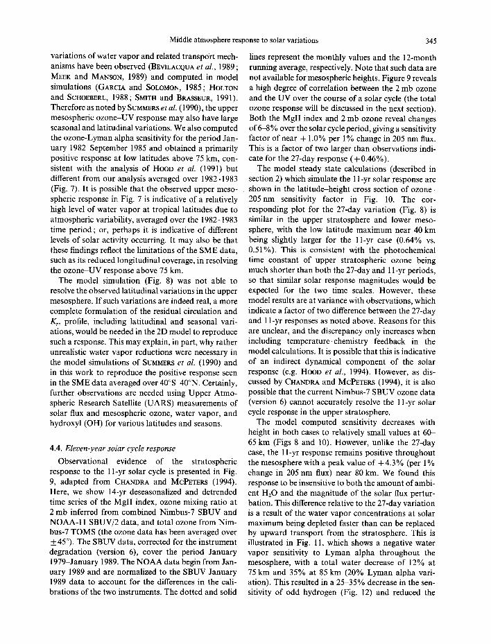
Observational evidence of the stratospheric response to the 11.-yr solar cycle is presented in Fig. 9, adapted from CHANDRA and MCPETERS (1994). Here, we show 14-yr deseasonalized and detrended time series of the MgII index, ozone mixing ratio at 2 mb inferred from combined Nimbus-7 SBUV and NOAA-11 SBUV/2 data, and total ozone from Nim- bus-7 TOMS (the ozone data has been averaged over _+ 45°). The SBUV data, corrected for the instrument degradation (version 6), cover the period January 1979-January 1989. The NOAA data begin from Jan- uary 1989 and are normalized to the SBUV January 1989 data to account for the differences in the cali- brations of the two instruments. The dotted and solid

345

lines represent the monthly values and the 12-month running average, respectively. Note that such data are not available for mesospheric heights. Figure 9 reveals a high degree of correlation between the 2 mb ozone and the UV over the course of a solar cycle (the total ozone response will be discussed in the next section). Both the MglI index and 2 mb ozone reveal changes of 6--8% over the solar cycle period, giving a sensitivity factor of near + 1.0% per 1% change in 205 nm flux. This is a factor of two larger than observations indicate for the 27-day response (+0.46%).

The model steady state calculations (described in section 2) which simulate the 11-yr solar response are shown in the latitude-height cross section of ozone- 205nm sensitivity factor in Fig. 10. The corresponding plot for the 27-day variation (Fig. 8) is similar in the upper stratosphere and lower mesosphere, with the low latitude maximum near 40 km being slightly larger for the 11-yr case (0.64% vs. 0.51%). This is consistent with the photochemical time constant of upper stratospheric ozone being much shorter than both the 27-day and 11-yr periods, so that similar solar response magnitudes would be expected for the two time scales. However, these model results are at variance with observations, which indicate a factor of two difference between the 27-day and 11-yr responses as noted above. Reasons for this are unclear, and the discrepancy only increases when including temperature-chemistry feedback in the model calculations. It is possible that this is indicative of an indirect dynamical component of the solar response (e.g. HOOD et al., 1994). However, as discussed by CHANDRA and McP~TERS (1994), it is also possible that the current Nimbus-7 SBUV ozone data (version 6) cannot accurately resolve the l l-yr solar cycle response in the upper stratosphere.

The model computed sensitivity decreases with height in both cases to relatively small values at 60- 65 km (Figs 8 and 10). However, unlike the 27-day case, the 11-yr response remains positive throughout the mesosphere with a peak value of +4.3% (per 1% change in 205 nm flux) near 80 km. We found this response to be insensitive to both the amount of ambient H20 and the magnitude of the solar flux perturbation. This difference relative to the 27-day variation is a result of the water vapor concentrations at solar maximum being depleted faster than can be replaced by upward transport from the stratosphere. This is illustrated in Fig. 11, which shows a negative water vapor sensitivity to Lyman alpha throughout the mesosphere, with a total water decrease of 12% at 75 km and 35% at 85 km (20% Lyman alpha variation). This resulted in a 25-35% decrease in the sensitivity of odd hydrogen (Fig. 12) and reduced the

346

t~

~3

>

5.0

2 .5

0.0

-2 .5

- 5 . 0


I I I I I I I I I I I I I

, . , . ~ ~o~ ~ ~ .S¢~..'..

I I I I I I I I I I I I I

5.0

2.5

0.0

-2.5

-5.0

~" 5.0 Z m 2.5 tD

"-" 0.0 o

- 2 . 5

- 5 . 0

I I I I I I i I I ! I I •

i i i siE.- , ,~ - : . - . "

5.0

2 .5

0.0

- 2 . 5

- 5 . 0

• : TOT OZONE .':. : .8 : t

o i N , , , , ~ 0 ~ ' : 'x~: : i t , . ,~e/: ~ ~ - 2 - ~ " -: ~- -~: : -. ~ - ~ 0

0 N - 1 - - 1 0

- 2 , , , , ~ , ~ :~ - 2 , E-

7 9 8 0 5 1 8 2 8 3 8 4 r 5 8 8 8 7 8 8 8 9 9 0 9 1 9 2 9 3

YEAR

Fig. 9. Time series for 13 yr of the MgII solar UV index (top), ozone mixing ratio at 2 mb inferred from combined Nimbus-7 SBUV and NOAA-11 SBUV/2 data as described in text (middle), and Nimbus-7 TOMS total ozone (bottom). The time series have been deseasonalized, detrended, and averaged over _+ 45 °. Dotted and solid lines represent the monthly values and the 12 month running average, respectively

(adapted from CHANDRA and MCPETERS, 1994).

catalytic HOx-ozone destruction relative to the 27-day variation (Fig. 4) in the middle mesosphere. Above 78 km, the large water vapor loss created a negative HO~-UV response (opposite to the 27-day variation) resulting in a large positive ozone response in this region.

Other model calculations of the 11-yr response (GARCIA et al. , 1984; HUANG and BRASSEUR, 1993) are similar to ours in the upper mesosphere with a large positive response maximizing near 80 km. How- ever, these studies computed a negative response at 65-75 km (the level of the minimum positive response we obtained in Fig. 10) and a maximum sensitivity in the upper stratosphere (+0 .2 -0 .23% per 1% 205 nm change) which was significantly smaller than we obtained ( + 0.64%). These differences are due in part to the fact that the GARCIA e t aL and HUANG and BRASSEUR models allow temperature to vary with solar flux, where as we did not allow for temperature-chemistry feedback. They reported solar maximum to solar

minimum temperature changes of + 1 to 3 K at 30- 75 km for low to middle latitudes, which induced a negative ozone response through the negative temperature-ozone coupling. To estimate the effects of temperature feedback for the 11-yr variation in our model calculations, we included the temperature response computed by the HUANG and BRASSEUR (1993) model as a function of altitude only (adapted from their Fig. 1 at low latitudes). We factored in the ratio of the 205 nm flux variations used in the two studies ( 3 % : 6 . 6 % ) giving, for example, an upper stratospheric response of 0.62 K. The resulting ozone response was reduced at all levels. The upper stratospheric maximum was + 0.35 % compared to + 0.64% with no temperature feedback (Fig. 10), although this was still larger than computed by the other models (+0 .2 to 0.23%). The response at 65-75 km became slightly negative ( - 0 . 0 1 % per 205 nm change), but was not as large as computed by the other models


E v

D

0. .

0 .01

0 . 1 0

1 . 0 0

1 0 . 0 0

1 C)O.O0

- 6 1

I I I I I I I I I I I

- 3 . 0 0 " 3 . 0 0 - - - 2.00

113o ~ " ~ 1 oo - 2 , 0 0 , _

- . . ~ ~ "~0..~~0"4n- • 0 . 3 0 ~ . , , u ~ "

- - 0.30 ~ ~ 0,30 -

"0.40 ~ ~ 0 .40"

- 0.50 - - - - 0.50 - -

- 0.60 ~ 0.60 "--------- _

- 0.150

0 . 6 0 - -

- 0 . 5 0 - - 0 , 5 0

~ 0 . 4 0 " ~ -0.40-

- 5 0 - 4 0 - 3 0 - 2 0 - 1 0 0 1 0 2 0 3 0 4 0 5 0

95

90

85

80

75

70,.-., E

6 5 ~

60

55 .<

50 >~

45 g 40 <

35

- 3 0

- 25

20

15

60

Fig. 10. Ozone-205 nm sensitivity as a function of latitude and height, derived from model computations for the 11-yr solar cycle variation.

0.01

9. I0 E

v

o . 1 . 0 0

1 0 . 0 0

) I l I I I I I I I I

~ 1 2 n ~ l a ^ ~ ' - " - - - 1 . 7 5 0 " . 0 0 t " . . . . t j " . . ~ - - " . ~ . . u O . " • ~-v 0 . . . . . ~ . . " . . . . . . . . . . . . . . . . . . . . . . . . . . . . . . . . ~ . b . . . . . . . . ~ . . . . . . . - ' ~ _ " . . . . . . . . . . . : : : : : : : : : : : : : : : : : : : : : : : : : : : : : : : : : : . o o o . . . .

~ - 0 . 8 0 0 ................. : .........................................................

. . . . . . 0 , 0 2 0

9 5

- 9 0

8 5

8 0

.--'.Z ............................................... r : : . ; - : . . . . . . . . . . . . . . . . . . . o 5oo .......... ~. ...._..-...!-: . . . . . . . . . . . : : . . . . ~ . k - 5 : T . - _ - - . . = = : : : - : = . - = : - o . 6 o ° . . . . . 7 5

....... ~ o ; " : : : : : : : : : : .................... :~- . . . . . . . . . . . . . . . . . . . . . . . . - . . . . . . . . . . . . . . . . . . . . . . . . :::~::4~:':: "-" .300 ......... ~ .................... - . . . . . . . . . . . . . . . . . . . . . . . . . . . : ............. - 7 0 ,,.,, . . . . . . . . . . . . . . . . . . . . . . . . . . . . . . . . . . . . . . . . . . . . . . . . . . . . . . . . . . . . . . . . . . . . . . . . . . . . . . . 0.200 ...... g : . . . . . . . 0.100 ......................................................... ~ ............................................. - 6 5

. . . . . . . . . . . . . . . . . . . . . . . . . . . . . . . . . . . . . . . . . . . . . . . . . . . . . . . . . . . . . . . . . . . . . . . . . . . . . . . . . . . . . . . . . . . . o .oso . . . . . . 6 0

-O.oio."

I I I I

2 0 3 0 4 0 5 0

E 1 0 0 . 0 0 F I I I I I I I

- 6 0 - 5 0 - 4 0 - 3 0 - 2 0 - 1 0 0 1 0

L o t i t u d e

-555 <

- 5 0 >~ £

- 4 5 a Ct. <

- 4 0

- 3 , 5

- 3 0

- 2 5

- 2 0

15

6O

Fig. 11. As in Fig. 10, but for the sensitivity of water vapor to Lyman alpha.


%-,

E v

n

0.01

0 .10

1.00

I ) [ I I I I I I 1 I

-0 .20 ............. ;Z-.-O.3o ... - .-. o . ~ ......................... _1.2 ......................... Z-Z... - o -,n ' ~ . 1 0 . . . . . . . . . . . . . . . . . . . . . . . . . . . . . :::::::::::::::::::::::::::::::::::::::::::::::::::::::: ........................... 0.10

% >

- O. 10 -----.. ~0.~ O /

" 0 . 0 8 ~ _-- - - - - - 0 . 0 6 "

- 0 .04 ~ . . - - - - 0 . 0 4 -

10.00 i.~~&OO ~ I -0.02 ~

" • - - . i I ) I I " - - - t

- 6 0 - 5 0 - 4 0 - 3 0 - 2 0 - 1 0 0 10 20 30 4-0

I

5O

95

190

85

80

75

70 ,.__.

6s~ 6O ~ ss~ 50 ~

4s ~ <

40

55

30

25

20 15

6O Latitude

Fig. 12. As in Fig. 10, but for the sensitivity of HOx (H + OH + HO2) to Lyman alpha.

(~ -0 .8%) . This result is consistent with our 27-day model simulation in which the negative ozone response at 65-75 km was enhanced when including the observed temperature response with a near-zero phase lag.

GARCIA e t al. (1984) and HUANG and BRASSEUR (1993) reported water vapor decreases from solar maximum to solar minimum throughout the mesosphere which were generally similar to ours (Fig. 1 l) in the sensitivity to Lyman alpha. Our computed HOx response (Fig. 12) was also in qualitative agreement with the other model results. Quantitatively, the GAR- CIA e t aL results indicate a HOx sensitivity to Lyman alpha which was a factor of 1.2-1.4 larger than we obtained in the middle mesosphere (Fig. 12) ; and the results of HUANO and BRASSEUR (1993) also indicate a somewhat higher OH-Lyman alpha sensitivity than we obtained. This would indicate larger UV induced catalytic HO,-ozone destruction which may con- tribute to the larger negative ozone response computed by the other models relative to ours in the 65- 75 km region.

Note finally that Fig. 10 shows significant differences with Fig. 8 in the lower stratosphere. This will be discussed in the context of the total ozone response in the next section.

5. T O T A L O Z O N E S O L A R R E S P O N S E

To investigate the observed 27-day UV response in total ozone, we computed the correlation between time series of daily Nimbus-7 TOMS data and the MgII solar index for the period 1989-1991 (corresponding to the solar cycle 22 maximum). Both time series were smoothed and deseasonalized as previously described. The resulting correlation coefficient plot is shown in Fig. 13 as a function of phase lag and latitude. The correlation is positive and independent of latitude throughout the tropics (30°S-20°N), with a maximum of +0.35. The phase lag at low latitudes is + 3 to 4 days and the sensitivity is + 0.11% 4-0.007, similar to the observations of CHANDRA (1991). The response and phase lag decrease with latitude poleward of the tropics in both hemispheres, with a near zero phase lag at 35-40 ° . This is indicative of the increasing importance of dynamical processes in con- trolling the total ozone distribution, as well as the solar response signal diminishing with the decreasing solar zenith angle.

The analogous total ozone-205 nm contour plot from the model simulations of the 27-day variation is shown in Fig. 14. The model reproduces the observed response quite well (again the correlation is generally


60

50

40

30

20

~0

~ o

~ -10

-20

-30

-40

-50

- 6 0

' _ o ~ . ,u- ~ u ~." -,o- • ~_

_ y ~ o ~ , , - - . . - . , \ t ~ ' ~ , ' " - : - - - ~ '

"0_ \ \ " x -- x ' ~ 0 * \ " #

,, (r(;': ',,, (M.+- ~ % ~ 1 t t I # I t - - ~- \ - t t v , , ~ t t \ t \ t\t~.;,,, , ,t\<f

M\ ;;x>,,,, ,:-,~A\\\ $Y4~",", ';',,k\~- '1 ~ / / 1 ,' "---",~:7 )~oo~)/I ', " ~ ; I l l

_- - - ~ * ' ~ 0 .00 o ~ .

6 0

50

40

30

20

lO ~

-10 ~

-20

-30

-40

-50

- 6 0

-50 -20 - 1 0 0 10 20 30 PHASE LAG (DAYS)

Fig. 13. Total ozone-MglI solar flux correlation coefficient as a function of phase lag and latitude, derived from deseasonalized Nimbus-7 TOMS data for 1989-1991. The MglI index (205 nm) is as described in the

text for the profile ozone response.

60 I I I t I 6 0

40 \ \ \ , , , % , ,,, &\ ,,',<," , 4o

,, ,~. ,, ,~<>.-,,

.,,,o..,~ .... i i~.-~,,,~-tl(((/(?¢, o ,,, 10 ,\\/111~,,<, ,, ,,,,////('c~'k\~[i,'

>- ")5><~),);)',',',':<V t; , ,~: . , , o

-~o o.~y/ , . - - - - - . . , ,~h---~{ t,~, -, .. "~Ato"~ \\ ~',, ",'< ,, -- ;-, .~o.

-~o ,,~ ~,,,,,, . , , ~ , ~ / ~ \ ~ \ , , ,, -..,o,~o~.:-~o

'°F , ',,,,.., , . . __., . o- 22 - ' ° . - so • i~., / . , ,5> .,?;,i?.7,;> 7 ~>.-:,/~TT;~.:~.,o ,.,, lv./s>~;,,~:,o -5o - 6 0 1 i i i i - 6 0

-30 -20 - 1 0 0 10 20 30 PHASE LAG (DAYS)

Fig. 14. Total ozone-205 nm solar flux correlation coefficient as a function of phase lag and latitude, derived from deseasonalized model calculations for the 27-day solar variation.

larger in the model). A positive response independent of latitude is seen throughout the tropics with a maximum correlation ( + 0.83) near the equator. Simi- lar to observations, the phase lag is about + 3 days, which corresponds 1:o an intermediate pressure level between 10 and 30 mb in the profile ozone response

(Fig. 6(b)). This is expected since total ozone at low latitudes is heavily weighted towards ozone concentrations in this altitude region. The sensitivity to solar flux at 205 nm is +0 .077% (per 1% solar flux change) which is slightly less than the + 0.11% indicated by observations (the model sensitivity increased

350 E. L. FLEMING et al.

only slightly to +0.085%, with no change in phase, when including the observed temperature response). As in the observations, the model correlation and phase lag decrease with latitude poleward of +_ 30 °. A secondary maximum with a near zero phase lag seen in the observations near 30°N (Fig. 13) was also simulated by the model, although at a higher latitude (45°N).

As shown in the bottom panel of Fig. 9, total ozone is observed to correlate well with the MgII index over the 11-yr solar cycle, with some interannual variations such as the QBO being evident. Solar max to solar min total ozone changes of 1.5-2% are observed, with a corresponding 6-8% change in 205 nm flux (MgII). The sensitivity factor of near +0.27% is 2-3 times greater than observed for the 27-day variation. CHAN- DRA (1991) attributed this difference to the photochemical time constant of ozone in the lower stratosphere which is comparable to the 27-day solar rotation period but is much shorter than the l l -y r solar cycle period. The model 11-yr simulations compare quite well with these observations, revealing a total ozone sensitivity factor at low latitudes of +0.27%, which is a factor of 3.5 greater than for the 27-day variation computed in the model. This is reflected in the comparison between Figs 8 and 10, which shows the lower stratospheric response being more strongly positive for the 11-yr variation (Fig. 10). As expected, the response value of +0.27% occurs at the level of maximum ozone concentration (30-10 mb in the tropics). The computed 11-yr total ozone-205 nm sensitivity was significantly larger than computed by HUANG and BRASSEUR (1993) (+0.10 to 0.12%) and GARCIA et al. (1984) (+0.18% for total column above 16 kin). Accounting for temperature feedback explained only part of this difference, as including this effect reduced our model sensitivity slightly to +0.23%.

6. CONCLUSIONS

We have used a 2D photochemical model to simulate the middle atmospheric response to the 27-day and 11-yr solar UV variations at low to middle latitudes. For the 27-day variation, the model reproduced most of the features of the observed sensitivity factors and phase lags of the response in the upper stratosphere and lower mesosphere, including the transition to a negative ozone-UV phase lag. We attribute this feature to the increasing importance with height of the solar-modulated HOx chemistry on the ozone response above 45 km. The model revealed strong UV responses of water vapor and HOx in the mesosphere,

and qualitatively reproduced the observed negative ozone response at 65-75 km. This feature was more accurately simulated when incorporating the observed temperature response in the calculations. However, adapting this methodology did not definitely improve the comparison with observations in the stratosphere. Accurate determination of the total temperature-UV response is necessary to ascertain the temperature- chemigtry feedback effect on the ozone response.

On an annual average basis, the model reproduced the general lack of latitudinal variability seen in the observed response at low to mid-latitudes in the 30- 75 km region. Consistent with the findings of SUMMERS et al. (1990), the upper mesospheric positive response observed in the SME data averaged over _+40 ° was simulated in the model only by reducing the ambient water vapor by more than an order of magnitude relative to recent ground based microwave measurements at midlatitudes (BEVILACQUA et al., 1989). This discrepancy may be indicative of natural variability or other processes occurring which are not accurately resolved in our present 2D model formulation, or it may reflect the limitations of current satellite measurements at such high altitudes. More observational analyses of the upper mesospheric solar response are needed as the UARS data becomes available.

Unlike the 27-day variation, the model revealed a positive ozone-UV response throughout the mesosphere for the 11-yr solar cycle, due to the large decrease of water vapor and subsequent decrease in HOx concentrations. Incorporating t empera tu re chemistry feedback in the model calculations produced a small negative ozone response at 65-75 km, and partially explained the discrepancy with previous theoretical studies of the 11-yr response in this region.

Consistent with the photochemical time scales in the upper stratosphere and lower mesosphere, the model simulations of the 11-yr solar cycle revealed a response similar to the 27-day variation in this region. For the 27-day response in total ozone, the model-computed sensitivity and phase lag were similar to observations. The computed 11-yr response was a factor of 3.5 larger than for the 27-day variation which is also consistent with observations and is indicative of the relatively long photochemical time constant of ozone in the lower stratosphere. Including temperature feedback in the model simulations of the 11-yr response seemed to lessen the agreement with observations in the upper stratosphere and for total ozone.

Acknowledgements--We would like to thank Michael E. Summers (Naval Research Laboratory), Lon L. Hood (Uni- versity of Arizona), and two anonymous referees for helpful discussions and comments concerning this work.


ALLEN M.,LUNINE J. I. and YuNGY. L.

ARNOLD F. and KRANKOWSKI D.

ATLAS E. L., RmLEY B. A., HUBLER G. WALEGA J. G., CABROLL M. A., MONTZKA D. D., HUEBERT B. J., NORTON R. B., GRAHEK F. E. add SCHAUFFLER S.

BEVILACQUA R. M., OLIVERO J. J. and CROSKEY C. L.

BEV1LACQUA R.M.,SrARK A. A. and SCHWARTZ P. R.

BEVILACQUA R. M., STROBEL D. F., SUMMERS M. E., OLIVERO J. J. and ALLEN M.

BEVILACQUA R. M., ~7ILSON W. J., RICKETTS W. B., SCHWARTZ P. R. and HOWARD R. J.

BRASSEUR G., DERUDOER A., KEATING G. i . and PITTS M. C.

BRA~EUR G. and SOLOMON S.

CHANDRA S.

CHANDRAS.

CHANDRAS.

CHANDRA S. and MCPETERS R. D.

CHANDRA S., McPETERS R. D., PLANET W. and NAGATANI R. ]X,[.

CIRA

CLANCY R. T., MUHLF.MAN D. O. and ALLEN M.

DELAND M. T. and CEBULA R. P.

DEMORE W. B., SANDER S. P., GOLDEN D. M., MOLINA M. J. HAM]?SON R. F., KURYLO M. J., HOWARD C. J. and ]RAVISHANKARA A. R.

DONNELLY R. F.

DOUGLASS A. R., JACKMAN C. n . and STOLARSKI R. S.

ECKMAN R. S.

ECKMAN R. S.

FLEMING E. L. and CHANDRA S.

REFERENCES

1984

1977

1992

351

The vertical distribution of ozone in the mesosphere and lower thermosphere. J. geophys. Res. 89, 4841- 4872.

Water vapour concentrations at the mesopause. Nature 268, 218-219.

Partitioning and budget of NOy species during the Mauna Loa observatory photochemical experiment. J. geophys. Res. 97, 10,449-10,462.

1989 Mesospheric water vapor measurements from Penn State: Monthly mean observations (1984-1987). J. geophys. Res. 94, 12,807-12,818.

1985b The variability of carbon monoxide in the terrestrial mesosphere as determined from ground-based observations of the J = 1 ~ 0 emission line. J. geophys. Res. 90, 5777-5782.

1990 The seasonal variation of water vapor and ozone in the upper mesosphere: Implications for vertical transport and ozone photochemistry. J. geophys. Res. 95, 883-893.

1985a Possible seasonal variability of mesospheric water vapor. Geophys. Res. Lett. 12, 397400.

1987 Response of middle atmosphere to short-term solar ultraviolet variations, 2. Theory. J. geophys. Res. 92, 903-914.

1984 Aeronomy of the Middle Atmosphere. D. Reidel, Hingham, Mass., U.S.A.

1984 An assessment of possible ozone-solar cycle relationship inferred from Nimbus-4 BUV data. J. geophys. Res. 89, 1373-1379.

1986 The solar and dynamically induced oscillations in the stratosphere. J. geophys. Res. 91, 2719-2734.

1991 The solar uv related changes in total ozone from a solar rotation to a solar cycle. Geophys. Res. Lett. 18, 837- 840.

1994 Solar cycle variations of ozone in the stratosphere. J. Geophys. Res. (in press).

1994 The 27-day solar uv response of stratospheric ozone : Solar cycle 21 versus solar cycle 22. J. atmos, terr. Phys. 56, 1057-1065.

1972 COSPAR International Reference Atmosphere. Aka- demie, Berlin.

1984 Seasonal variability of CO in the terrestrial mesosphere. J. #eophys. Res. 89, 9673-9676.

1993 The composite Mg II solar activity index for solar cycles 21 and 22. J. geophys. Res. 98, 12,809-12,823.

1990 Chemical kinetics and photochemical data for use in stratospheric modeling. JPL Publ. 90-1, 217 pp.

1991 Solar UV spectral irradiance variations. J. geomag. Geophys. 43 (Suppl.), 835-842.

1989 Comparison of model results transporting the odd nitrogen family with results transporting separate odd nitrogen species. J. geophys. Res. 94, 9862- 9872.

1986a Response of ozone to short-term variations in the solar ultraviolet irradiance, 1. A theoretical model. J. geophys. Res. 91, 6695-6704.

1986b Response of ozone to short-term variations in the solar ultraviolet irradiance, 2. Observations and Interpre- tation J. geophys. Res. 91, 6705-6721.

1989 Equatorial zonal wind in the middle atmosphere derived from geopotential height and temperature data. J. atmos. Sci. 46, 860-866.

352

FLEMING E. L., CHANDRA S., BARNETT J. J. and M. CORNEY

GARCIA R. R. and SOLOMON S.

GARCIA R. R., SOLOMON S., ROBLE R. G. and RUSCH D. W.

GROSSMAN K. U., FRINGS W. G., OFFERMAN D., ANDRE' L., KoPP E. and KRANKOWSKY D.

HEATH D. F. and SCHLESINGER B. M.

HERMAN J. R., HUDSON R.,McPETERS R., STOLARSKI R.,AHMAD Z. ,Gu X.-Y., TAYLOR S. and WELLEMEYER C.

HOLTON J.R. and SCHOEBERLM. R.

HOOD L. L.

HOOD L. L.

HOOD L. L. and DOUGLASS A. R.

HOOD L. L., HUANG Z. and BOUGHER S. W.

HOOD L. L. and JIRIKOWIC J. L.

HOOD L. L., JIRIKOWIC J. L. and MCCORMACK J. P.

HUANG T. Y. W. and BRASSEUR G. P.

JACKMAN C. H., DOUGLASS A. R., BRUESKE K. F. and KLEIN S. A.

JACKMAN C. H., DOUGLASS A. R., ROOD R. B., MCPETERS R. D. and MEADE P. E.

KEATING G. M., PITTS M. C., BRASSEUR G. and DERUDDER A.

KoPP E.

KtmzI K. F. and CARLSON E. R.

LAURENT J., BRARD D., GIRARD A., CAMY-PEYRET C., LIPPENS C., MULLER C., VERCHEVAL J. and ACKERMAN i .

LEAN J.

MATSUNO T.


1990 Zonal mean temperature, pressure, zonal wind and geopotential height as functions of latitude. Adv. Space Res. 10, 11 59.

1985 The effect of breaking gravity waves on the dynamics and chemical composition of the mesosphere and lower thermosphere. J. geophys. Res. 90, 3850-3868.

1984 A numerical response of the middle atmosphere to the 11-year solar cycle. Planet. Space Sci. 32, 411423.

1985 Concentrations of H20 and NO in the mesosphere and lower thermosphere at high latitudes. J. atmos, terr. Phys. 47, 291-300.

1986 The Mg-280 nm doublet as a monitor of changes in solar ultraviolet irradiance. J. #eophys. Res. 91, 8672- 8682.

1991 A new self-calibration method applied to TOMS/SBUV backscattered ultraviolet data to determine long term global ozone change. J. #eophys. Res. 96, 7531-7545.

1988 The role of gravity wave generated advection and diffusion in transport of tracers in the mesosphere. J. geophys. Res. 93, 11,075-11,082.

1986 Coupled stratospheric ozone and temperature response to short-term changes in solar ultraviolet flux. J. geophys. Res. 91, 5264-5276.

1987 Solar ultraviolet radiation-induced variations in the stratosphere and mesosphere. J. #eophys. Res. 92, 876-888.

1988 Stratospheric response to solar ultraviolet variations: Comparisons with photochemical models. J. 9eophys. Res. 93, 3905-3911.

1991 Mesospheric effects of solar ultraviolet variations : Fur- ther analysis of SME IR ozone and Nimbus-7 SAMS temperature data. J. #eophys. Res. 96, 12,989-13,002.

1991 Stratospheric dynamical effects of solar ultraviolet variations: Evidence from zonal mean ozone and temperature data. J. #eophys. Res. 96, 7565-7577.

1993 Quasi-decadal variability of the stratosphere : Influence of long-term solar ultraviolet variations. J. atmos. Sci. 50, 3941 3958.

1993 Effect of long-term solar variability in a two-dimensional interactive model of the middle atmosphere. J. #eophys. Res. 98, 20,413 20,427.

1991 The influence of dynamics on two-dimensional model results : Simulations of 14C and stratospheric aircraft NOx injections. J. #eophys. Res. 96, 22,55952,572.

1990 Effect of solar proton events on the middle atmosphere during the past two solar cycles as computed using a two-dimensional model. J. #eophys. Res. 95, 7417- 7428.

1987 Response of middle atmosphere to short-term solar ultraviolet variations, 1. Observations. J. yeophys. Res. 92, 889-902.

1990 Hydrogen consistuents of the mesosphere inferred from positive ions : H20, CH4, H2CO, H202, and HCN. J. #eophys. Res. 95, 5613-5630.

1982 Atmospheric CO volume mixing ratio profiles determined from ground-based measurements of the J = 1 --* 0 and J = 2 --* 1 emission lines. J. geophys. Res. 87, 7235-7241.

1986 Middle atmospheric water vapor observed by Spacelab One grille spectrometer. Planet. Space Sci. 34, 1067- 1071.

1987 Solar ultraviolet irrdiance-induced variations: A review. J. 9eophys. Res. 92, 839-868.

1970 Vertical propagation of stationary planetary waves in the winter northern hemisphere. J. atmos. Sci. 27, 871-883.

MEEK C. E. and MANSON A. H.


1989

OORT A. H.

PLANET W. G., LIENE.';CH J. H., MILLER A. J., NAGATANI R., MCPETERS R. D., HILSENRATH E., CEBULA R. P., DELAND M. T., WELLEMEYER, C. G. and HORVATH K. M.

REINSEL G. C., TIAO G. C., AttN S. K., PUGH M., BASU S., DELUISI J. J., MATEER C. L., MILLER A. J., CONNELL P. S. and WUEBnLES D. J.

REINSEL G. C., TIAO G. C., MILLER A. J., WUEBBLES D. J., CDNNELL P. S., MATEER C. t . and DELUISI J. J.

ROSENFIELD J. E., SCHOEBERL M. R. and GELLER M. A.

RUSSELL J. M. 1II, GILLE J. C., REMSBERG E. E., GORDLEY L. L., BAILEY P. L., FISCHER H., GIRARD A., DRAYSON S. R., EVANS W. F. J. and HARRIES J. E.

SELLERS W. D.

SMITH A. K. and BRASSEUR G. P.

STORDAL R., ISAKSEN I. S. A. and HORNTVETH K.

STROBEL D. F., SUMMERS M. E., BEVILACQUA R. M., DELAND M. T. and ALLEN M.

SUMMERS M. E., STROBEL D. F., BEVILACQUA R. M., ZHU X., DELAND M. T., ALLEN M. and KEATING G. M.

THOMPSON A. M., HUNTLEY M. A. and STEWART R. W.

THOMPSON A. M., JOHNSON J. E., TORRES A. L., BATES T. S., KELLY K. C., ATLAS E., GREENBERG J., DOI~AHUE N. M., YVON S., SALTZMAN E., HEIKES B. G., NOSHER B. W., SHASHKOV A. A. and YEGOROV V. I.

THOMPSON A. M. and STEWART R. W.

353

Vertical motions in the upper middle atmosphere from the Saskatoon (52°N, 107°W) M. F. radar. J. atmos. Sci. 46, 849-858.

1983 Global Atmospheric Circulation Statistics, 1958-1983. NOAA Prof. Paper 14.

1994 Northern hemisphere total ozone values from 1989- 1993 determined with the NOAA-11 solar back- scatter ultraviolet (SBUV/2) instrument. Geophys. Res. Lett. 21, 205-208.

1988 An analysis of the 7-year record of SBUV satellite ozone data: Global profile features and trends in total ozone. J. geophys. Res. 93, 1689-1703.

1987 Statistical analysis of total ozone and stratospheric umkehr data for trends and solar cycle relationship. J. geophys. Res. 92, 2201-2209.

1987 A computation of the stratospheric diabatic residual circulation using an accurate radiative transfer model. J. atmos. Sci. 44, 859-876.

1984 Validation of water vapor results measured by the limb infrared monitor of the stratosphere experiment on Nimbus-7. J. geophys. Res. 89, 5115-5124.

1965 Physical Climatology. The University of Chicago Press, Chicago, U.S.A.

1991 Numerical simulation of the seasonal variation of mesospheric water vapor. J. geophys. Res. 96, 7553- 7563.

1985 A diabatic circulation two-dimensional model with photochemistry: Simulations of ozone and long- lived tracers with surface sources. J. geophys. Res. 90, 5757-5776.

1987 Vertical constituent transport in the mesosphere. J. geophys. Res. 92, 6691-6698.

1990 A model study of the response of mesospheric ozone to short-term solar ultraviolet flux variations. J. #eophys. Res. 95, 22,523-22,538.

1990 Perturbations to tropospheric oxidants, 1985-2035, 1. Calculations of ozone and OH in chemically coherent regions. J. geophys. Res. 95, 9829-9844.

1993 Ozone observations and a model of marine boundary layer photochemistry during SAGA-3. J. geophys. Res. 98, 16,955-16,968.

1991

WATERS J. W., WILSON W. T. and SHIMABOKURO F.I. 1976

WORLD METEOROLOGICAL ORGANIZATION (WMO) 1990 WORLD METEOROLOGICAL ORGANIZATION (WMO) 1992

Reference is also made' to the following unpublished material: REMSBERG E. E., RUSSELL J. M. III and Wv C.Y. 1989

Effect of chemical kinetics uncertainties on calculated constituents in a tropospheric photochemical model. J. geophys. Res. 96, 13,089-13,108.

Microwave measurement of mesospheric carbon monoxide. Science 191, 1174-1175.

WMO Rep. 20, Washington, D.C. WMO Rep. 25, Washington, D.C.

An interim reference model for the variability of the middle atmosphere H20 vapor distribution. Hand- book for Middle Atmosphere Program 31, 50-66.

APPENDIX A

Model validation~data comparison

In this paper, we have presented for the first time, results using our model which has recently been upgraded to include: mesospheric heights (60-90 km), computed water

vapor, and improved eddy diffusion formulations (Kyy, K z ~ see Appendix B). To provide a general comparison with observations, we present steady state model simulations in the middle atmosphere along with various climatological data bases of ozone and water vapor. We emphasize the mesosphere in our comparisons and also include carbon

354

v

L~

t / ) U l L~ n,, 13-

0 .001

0 . 0 1 0

0 . 1 0 0


MODEL OZONE (ppmv) DECEMBER I I I I I [ I I I I I

o~O/ ~

- 0 . 3 0 - - . - - - - - - 0 . 2 0 - - <-- 0 . 2 0 "

0 . 3 0 -

- 0 . 4 0 - - 0 . 5 0 - - ~ . 6 0

1 . 0 0 -

- 1 . 3 0 - 2 . 0 0 -

1 . 0 0 0 ~ ~ 3 . o o - - 3 . 0 0 -

4 . 0 0 - ~ .5.00 ~ ----. . ._ "vO.

.'1.u ~ ~ - - - . - - - - ~ ~ ~,6' "vO oooo "

:~:RR . - - - - - - - - - - - - - ~ s.oo- ,

1 0 0 . 0 0 0 ~.~o I i ~ - - . ~ " T " " ~ f O"

- 6 0 - 5 0 - 4 0 - 3 0 - 2 0 - 1 0 0 10 20 3 0 40 5 0 LATITUDE

95

90

85

8 0

75

70 ~ 65"j 60 ~

i . . - 55 ~ 50 <

X ,,5 o

O_ 40 ca_

35

30

25

20 15

60

Fig. A-1. Latitude-height cross section of ozone mixing ratio (ppmv) for December, from baseline steady state model computations.

OBSERVATIONS OZONE 0 .001 I 1 1 t F t

0 . 0 1 0

~E v

w

::D t / )

0 . 1 0 0

. . . ~ 0 . 4 0

~ " " O. ~ 5 - ~ _ _

"-'----'-----0.20 - y. - o.3o 0.40 - ~ 0 . 6 0

_ ~ . o o ~ - - ~ :

1 . 5 0

0 . 3 0 -

(ppmv) DECEMBER i i i i i [ 9 5

-190

.o.,o

_ o

_ _ _ . . . ~ - o 3o ~.,d 6s

tn _2.oo- -E.oo ~ S . g O 3 ° ~ 50 x ' " 1 . 0 0 0 "" ~oo------ ~ " - ' 4 5 o

"-- ~:OU -- l~.OO u~

, , ~ ~ _ _ s . 0 o ~ I- 40 o_

~ c. o ~ . . . . . . _ _ ~ ~ ~ . ~ 1 .°" .~.oo ~ / ,-} ,-' 1 0 . 0 0 0 - - . o o . . . . . . . ~ ~ ~ - 30

5 . 0 0 ~ 4"---"~'E-° s ' ° ° 3. o o . - " - " " ' - " ~ . ~ 2 5

2O 1 0 0 . 0 0 0 t I I I t J J L t l I 1 5

- 6 0 - 5 0 - 4 0 - 3 0 - 2 0 - 1 0 0 1 0 20 3 0 4 0 5 0 60 LATITUDE

Fig. A-2. Latitude-height cross section of ozone mixing ratio (ppmv) for December, based on Nimbus-7 SBUV data for 30-1 mb averaged over 1979-1986, and SME IR data for 0.75-0.0056 mb averaged over

1982-1985.

monoxide (CO) which is important in this region and for which some limited observations are available. Note that we exclude model results above 85 km which are strongly influenced by the top boundary (~ 90 km).

Ozone. Latitude-height cross sections of model ozone are

shown in Fig. A-I, along with climatological observations (Fig. A-2) for solstice conditions (December), based on: Nimbus-7 SBUV data for 30-1 mb averaged over the period t979-1986; and the Solar Mesosphere Explorer (SME) satellite infra-red measurements for 0.75~).0056 mb averaged

'I 355

0.01

v 0.10

1.00

"10.00

100.00 0.1


OZONE ( p p m v ) 5°N DECEMBER , , i , i , , I i i

i/"

......... SIdE UV

,~, ~2D Model

J l I P " ~ l I I I I I I I I I I I I I

1 PPMV

' 95

- 9 0

- 85

80

75

70

6 5 f f

6 o ~ ,

50

45 <

40

35

3O

25

2O

15

10

Fig. A-3. Vertical profiles of ozone mixing ratio from model computations and climatological observations as given in Fig. A-1 and A-2, for December at 5°N. Climatological SME UV ozone data from 1982-1985

for 1~). 1 mb are also included.

over 1982-1985. The model reproduces the basic features seen in the observations such as the middle stratospheric maxima near 10 mb, and the minima in the middle mesosphere at 70-75 km. Note also the general lack of latitudinal variation in the uptx:r stratosphere and lower mesosphere seen in both model and data.

Figures A-3 and A-4 show vertical profiles of model and observational ozone for December at 5°N and 45°N, respectively. In addition to the data sets described above, we also include climatological SME UV ozone measurements from 1982-1985 for 1-0.1 nab. Again, the model reproduces the general structure seen in the data. The model at 5°N over- estimates the ozone value above 65 km, although the level of minima at 70 km is similar to observations. The comparison in the mesosphere is generally better at 45°N.

Figures A-5 and A-6 show the monthly variations of ozone from the model and observations at 5°N and 45°N for three mesospheric levels corresponding to approximately 55, 70, and 85 km (0.5, 0.05, and 0.005 mb---we interpolated all observations and model output to identical pressure surfaces). At 55 kin, the model shows a qualitatively similar seasonal variation to. the data at both latitudes, with the seasonal amplitude and absolute magnitude of the model being somewhat less. The model simulation at 70 km compares fairly well with the data, although the seasonal amplitude of the model is slightly larger at 45°N. The dominant semiannual cycle amplitude and phase at 85 km are reproduced quite well in the model at 45°N, although the absolute value (annual mean) of the observations is 25% higher. At

5°N (85 km), the model compares well in terms of semiannual amplitude and annual mean ; however the semiannual phase of the model is offset by 2 months.

Note that the model generally underpredicts the ozone observations in the lower mesosphere (e.g. 55 km), and over- predicts ozone in the middle mesosphere (e.g. 70 km), while the opposite is true for water vapor (see Figs A-11 and A- 12). This is consistent with the observation that the ozone concentrations in the lower and middle mesosphere are controlled primarily by HOx chemistry, and therefore are anti- correlated with HOx and H20 amounts.

Water vapor. Figures A-7 and A-8 show latitude-height cross sections of water vapor for December and April computed from the model (see section 3 for details of the model water vapor computation). Corresponding climatological observations for April are shown in Fig. A-9, which are based on values from OORT (1983) for the troposphere and Nimbus-7 LIMS data for the stratosphere (e.g. RUSSELL et al., 1984). The values for the mesosphere (50-90 km) are adapted from the H20 profile of SUM~Cm~ et aL (1990), which was independent of season and latitude and represents the average for April-June 1984 of ground based microwave measurements at JPL (34°N Iatitude--BEWLACQUA et al., 1985a). Note that our model values are fixed to the values of OORT (1983) below 400 mb, and are therefore identical to the observational values at these levels. The model simulated water vapor compares fairly well with the observations in reproducing the general climatological structure, such as the tropical tropopause minima and the broad maxima in the

356

v

w n, , "

W rK O_

0.01

0.10

1 . 0 0

10.00

1 0 0 . 0 0 E_

0.1


OZONE (ppmv) 45°N i i P J ' J ' I

DECEMBER q i I

f

Nimbus-7 £BUV - - - - - - SME IR

.......... SME UV ~2D Model

1 PPMV

Fig. A-4. Same as Fig. A-3, but for 45°N.

. . . . t9590

85

75

70

65

-6o~ -55 c~

- 5 0 ~ <

- 4-5

4-0

35

30

25

- 20

_ 1 5

10

upper stratosphere and lower mesosphere, as well as their relative magnitudes. The model also reproduces the decrease of water vapor mixing ratio with increasing height throughout the middle and upper mesosphere (climatological water vapor observations in the mesosphere are not available for December).

Vertical profiles of stratospheric water vapor from the model and Nimbus-7 LIMS data (REMSBE]{G et al., 1989) for April are shown for the tropics (a) and southern hemisphere midlatitudes (b) in Fig. A-10 (mesospheric H20 observations for these latitude zones are currently not available). The model in the tropics compares well with the general structure exhibited by the observations, although the model values are systematically 15-30% larger. At southern midlatitudes, the model values are less in the lower stratosphere and greater in the upper stratosphere, with a corresponding steeper vertical gradient throughout the stratosphere. Note that the model accurately simulates the level of the water vapor minimum in the southern midlatitude lower stratosphere.

Figure A-l l shows vertical profiles (stratosphere and mesosphere) of observations from the Northern hemisphere midlatitude interim reference profile for spring (RBMsBERG et al., 1989) which is based on LIMS data for the stratosphere and various ground based microwave water vapor measurements between 35°N and 45°N for the mesosphere, and the empirical mesospheric water vapor profile of SUMMERS et al. (1990) mentioned above. Again, the corresponding model computations reproduce the general vertical structure of the observations, while being systematically larger throughout the stratosphere and lower mesosphere as in the tropics.

However, the model exhibits a systematic underestimation of the observations above 60 km, as was mentioned in the discussion of model ozone in relation to HOx-ozone chemistry in the mesosphere.

The model vertical K= profile in the stratosphere and mesosphere, which is independent of latitude and season, was determined in large part by achieving a vertical water vapor distribution which agreed as closely as possible with observations throughout the model domain. However the systematic biases seen in Figs A-10 and A-11 show latitudinal and seasonal variations. Future model improvements will provide an improved simulation of the vertical eddy diffusion which contains latitudinal and seasonal variations.

Referring again to the December simulation cross section of Fig. A-7, the model reveals a distinct latitudinal variation of water vapor in the mesosphere, with values at middle and high latitudes being larger in the summer hemisphere than in winter. This is indicative of the upward residual circulation in the summer hemisphere, which transports water vapor- rich air up from the stratosphere, and the downward transport of drier air from the upper mesosphere/lower thermosphere in winter. Previous observational analyses have reported a similar substantial seasonal variation in mesospheric water vapor (e.g. BEVILACQUA et al., 1990; SUMMERS et aL, 1990; SMITh and BRASSEUrt, 1991). This variation is seen in the monthly profiles of model and observed water vapor near 40°N at three mesospheric levels (65, 70, and 80 km--Fig. A-12). The data are from ground based microwave measurements at the Pennsylvania State University (Penn State) (41°N) and the Jet Propulsion Laboratory


1.0

0.8

0.6

0 .4

0.2

0.0

¢- ~ 1.0

v 0.8 0

~ 0.6

c 0.4.

=E 0.2 I-,J

Z 0.0 N o

1.0

0.8

0 .6

0.4

0 .2

0 .0

D

1.0

0.8 "-~ O

0.4 2~

0.2 ~

0,0 ~ N

OZONE (ppmv) 5°N ' ' ; ' ' ' ' ' ' 85' km

I I I I I I I I I I

F M A M J J A S 0 N

I N l m b u ~ - 7 SBUV' ' ' ' ' 7 0 ' k r n

- - - - - SME IR

. . . . . . . SME UV

~ 2 D Model

._ = = _ _ _ = . _ _ ~ - _ _ - , ~ , - ~ - ~ =

I I l I I I I I I I

F d M A M d J A S 0 N D o

2.2 ' ' ' ' ' ' ; ' ' 55 tkrn 2.2

2.0 ................................................... ..-.. 2.0

1.8 ~ _ - - ~ " ~ - - - - " " - ~ " ~ - ~ - 1.8

1.6 -- ---- ~'" 1.6

1 . 4 1 . 4

1 . 2 I I I I I I I I I I 1 . 2

F M A M J J A S 0 N O MONTH

Fig. A-5. Seasonal variations of ozone mixing ratio from model computations and climatological observations at 5°N for ~ 55, 70, and 85 km (0.5, 0.05, and 0.005 mb). The model and data are as in Fig. A-3,

and all values have been linearly interpolated to identical pressure surfaces.

357

(JPL) (34°N) (BEVILACQUA et al., 1989, 1990). Note that the months run from November to October. At 70-80 km the model reproduces the general seasonal variation of the data described above, with a winter minimum and summer maximum. The model at 70 km does indicate a minimum during April-May which is not seen in the data. At 65 km, the observations show relatively little seasonal variation, whereas the model reveals a spring minimum with a sharp increase to a late summer maximum.

We also present similar figures for two stratospheric levels (10 and 1.5 mb), for the northern hemisphere midlatitudes using Nimbus-7 LIMS data for comparison (Fig. A-13). Both model and data show very small seasonal variations at both levels. The figure also reveals the systematic bias described previously, with the model water vapor being consistently larger than seen in the data. This was postulated as being due in part to a lack of seasonal and latitudinal variations in our K= formulation. It is also possible that stratospheric water vapor has increased over the past 10-15 yr due to anthropogenic increases in methane emissions at the ground. Such increased methane amounts would, upon reaching the stratosphere, photolyze and provide for an

increase in stratospheric water vapor. Given a 1% per year increase in ground-based methane emissions during the past 10-15 yr (WMO, 1992), we estimate a corresponding 5-10% increase in stratospheric H20. This additional source of water vapor could account in part for the differences seen in Fig. A-13, since the LIMS data is from 1979, whereas the model uses boundary conditions for methane corresponding to 1990.

Carbon monoxide. Figure A-14 shows a latitude--height cross section of model computed carbon monoxide (CO) for December. Carbon monoxide is primarily significant in the mesosphere, and exhibits a general decrease with decreasing height away from its source region in the lower thermosphere. A significant seasonal variation exists in the mesosphere with a summer hemisphere minimum caused by the residual circulation transport of small CO concentrations up from the stratosphere, and a winter hemisphere maximum induced by large CO transport down from the lower ther- mospheric source region. These results are consistent with the observations of CLANCY et al. (1984).

Figure A-15 shows vertical profiles of the model CO at 40°N compared with ground based microwave observations

358

1.0

0.8

0.6

0.4

0.2

0.0

1.0 0.. " " 0.8 0 :,,.-., o 0.6 O~ :_~ o.4

tu 0.2 Z o 0.0 a 0

2,2

2.0

1,8

1.6

1.4-

1,2


OZONE (pprnv) 45°N ' ' ' ' ' g ~ ' 85 ~ krn

I I I I I I I I I I

F M A M J J A S 0 N

I N i m b u S - 7 SBUV . . . . ~ 7 0 ' k i n - - - - SME IR

. . . . . . . SME UV ~ 2 D Model

I I I I I I I I I I

F M A M d d A 5 0 N

1.0

0 .8

0.6

0 .4

0.2

O.O

D

1.0 o..

0 .8" - ' o

0.6 ~

0,4 ,_c x

0 .2 ,,, Z

0 . 0 o N

D o

I i I i I I i I I I , '-. . 55 .k~..

I I I I I I I I I I

2.2

2.0

1.8

1.6

1.4

1.2

M A M J J A S 0 N D MONTH

Fig. A-6. Same as Fig, A-5, but for 45°N.

for single days during late January 1982 (bottom) and April 1984 (top) (BEWLACQUA et al., 1985b), and February and March 1979 (bottom) (KuNzl and CARLSON, 1982). These measurements were taken at the AT&T Bell Laboratories Observatory in Holmdel, New Jersey (40°N). We have also included measurements taken in E1 Segundo, California (34°N) during April and May 1975 (Fig. A- 15, top) (WATERS et al., 1976). The model compares fairly well with the observations in reproducing the general characteristics of the vertical CO distribution, The model and data show particularly good agreement for the April case. The observations during the winter months show a good deal more variation, although the model profile does fall in between the two observational profiles. The limited data base currently available precludes us from showing more detailed comparisons of the vertical profiles and seasonal variations of model CO.

As data from the Upper Atmospheric Research Satellite (UARS) becomes available, further validation will be made of the model generated fields of ozone (MLS, HALOE, ISAMS, CLAES), water vapor (MLS, HALOE, ISAMS, CLAES), and CO (ISAMS), as well as other constituents in the mesosphere.

APPENDIX B

Calculation o f a consistent Kyy

The eddy diffusion coefficient (Kyy) is calculated from the relationship :

f~* - a, Kyy - (1) q,

Here, f is the Coriolis parameter, ~* the residual mean meridional circulation, a the zonal mean wind, and q the potential vorticity. Equation (1) is obtained by combining the zonal mean momentum equation,

at - f ~ * = v" q" + M , (2)

and the assumption that the eddy potential vorticity flux v'q ~ and the meridional potential vorticity gradient are con- nected by a flux~gradient relationship :

v'q' = - Kryt7 r . (3)

In order to arrive at equation (1) using equations (2) and

0.001


MODEL H20 (ppmv) DECEMBER I I I I ] 95

90

O . O L O - , . o ~ o o ~ ~ 80 • .o0.~. 75

o.loo - - " - : ~ ~ _ _ 6s m" 6 0 ~ "

s s ~ ' " 50 ~_ "" 1.000 - = oo._ 4s .~ 03

,., 40 x o: o_ 35 o

lO.0OO - 30 ~_ ~.Oo 25 <

1 0 0 , 0 0 0 ~ 8 ~ . . ~ . 1 ~ ~ ~ ~ 1 0 . 0 0 - _ ~ 15

1000o000 0

- 9 0 - 6 0 - 3 0 0 30 60 90 LATITUDE

Fig. A-7. Latitude-height cross section of water vapor mixing ratio (ppmv) for December from baseline steady state model computations.

359

i,i

O'} kd t~ 12t.

0.001

0.010

0.100

1.000

10.000

100.000

1000.000

- 9 0

M O D E L H 2 0 ( p p m v ) A P R I L , , , , , / 9 5

_~.ooO.SO ~ o . 2 o - o . 1 o - . ~ o.os _ ~ 90 85 • ° ' -

_ , . o o - 4 . o o ~ - - . . . . . . ~ ~ ~ - 1.oo - ~ o . /

5 O0 • - . ~ ~ - ' % ~ ~ - ] 7 o _.

~ ' 6 0 0 " ~ 5 5 - 5 0 ___

~ o . ~ , , T- ~ 5 o o p . o o _ = ~ - ' T - - - ~ ' " - ~ - ~ . c / 0 - 6 0 - 3 0 0 3 0 6 0 90

LATITUDE Fig. A-8. Same as Fig. A-7, but for April.

1- 45 .,~ 40 x 35 o

n 30 o. 25 <

360

v W :D

03 L~ rv' 0..

0.001

0 .010

0.100

1.000

10.000

100.000

1000.000


OBSERVATIONS H20 (ppmv) APRIL I I I I

- -0 .5 - - - - 1 . 0 - -

- - 2 .0 - -

--3.0 - -

- - 4 . 0 m

I

- < - - - - - - > -

F o----3 5.0

95 90

85

80

75

70,,_,,

65 60 v

I.d

55 50 _ 45 40 × 35 o 3o 25 < 20 15 10

o - 9 0 - 6 0 - 3 0 0 30 60 90

LATITUDE Fig. A-9. Lat i tud~height cross section of water vapor mixing ratio (ppmv) for April, derived from various climatological observations : OORT (1983) for the troposphere, Nimbus-7 LIMS data for the stratosphere, and ground based microwave measurements at JPL (34°N) averaged over April-June 1984 for 50-90 km.

E

(2-

10

o) 1 O0

0 1

H20 (ppmv) APRIL

zs~ j A ~ ~ Model 25"S-25"N 30 ~

LIMS 28*S-28*N 25 ;

2O < 15

3 4 5 6 7 8 9 10

50 ( ) SH Midlots 45

& y 4 0 ~

'~ 10 35

i zo 25 ~.

/ I - - Model 3 5 " S - 5 5 " . o_ b) ~ L --.,,MS ~ 2 " s - s e - s 20 100 , ~ "~ . . . . , 1 5

1 3 4 5 6 7 8 9 0 H20 (ppmv)

Fig. A- 10. Vertical profiles of stratospheric water vapor from the model as in Fig. A-8, and Nimbus-7 LIMS data for April in the (a) tropics, and (b) southern hemisphere mid-latitudes,

averaged over the latitudes indicated.

(3), the unspecified source of zonal momentum M (such as from gravity waves) is assumed to be negligible.

In order to obtain K)y from equation (1), the meridional wind 0* is obtained from the vertical wind by continuity. The zonal mean wind, tT, is calculated from the thermal wind relationship,

R k.-

~7~ = - 7 ~ e "0y, (4) j r l

where R is the gas constant, H a mean scale height, k = R/G, and 0 is the potential temperature. The assumption that a = 0 at the ground is used. At the e q u a t o r f ~ 0, so equation (4) is invalid. A valid relationship for the equatorial region is obtained from the meridional and vertical derivatives of the geostrophic wind equation, fu = - O y :

fu~: + #u~ = - 4%,.. (5)

Here, qb is the geopotential, and fl = f~.. The hydrostatic bal- ance equation, @: = R T / H , gives :

• R =y,, = ~ Tyy . (6)

This is combined with equation (5) to obtain, in the zonal average,

R _ k z -

tT: = -- -dTi~e ~0)~.. (7) p/7

v laJ

,93 la.I [3£

0.001

0.010

0.1 DO

1 . 0 0 0

I 0.000

Middle a tmosphere response to solar variations

H20 ( p p m v )

- - MODEL 4O°N - - - - - S p r i n g NH Midlaf Ref Profile ........... Summers ef al. ( 1 9 9 0 )

100.000 . . . . . . . . i

0.1 1.0 10.0 H20 (ppmv)

............................ ,.~<L .....

--'~.

- _ • . !

) t \

I !

I 'l I

J /

! i i i ' % i

' ' ' | 9 5

, 90

85

80

75

- 7 0

" 6 5 ' ' " laJ

60 ~ F-,.

55 ~,

50 < X

45 o 40 ~ 35

30

25

20 , , 15

Fig. A-11. Vertical profiles of modeled water vapor at 40°N averaged over Apr i l - June ; the spring nor thern hemisphere midlatitude reference profile of REMSB~RG et al. (1989) ; and the mesospheric profile of SUMMERS

e t al. (1990).

361

H20 ( p p m v ) 40°N

I . . . . . . . . ' 8 0 l ~ m

2 . . . . . . . . . . . . . . . . ; : / ............................ i / /

1

Ol ~ l i ~ l i , I I i

N D J F M A M J J A S

81 ' "6DEL''O°A . . . . . ~0 ~,,, 18 7 I - - - - - OBS Penn Sfa*e (41°N) 1 7 ~ , 6 ~ ......... OBS JPL (34°N) ." / " -]6 E

o 4L~,. ............... > . . . . . . . =.~ / _t4o

1 N D J F M A M J J A S 0

8 . . . . , 5 m8 7 / / ~ ~ 7

6 - - - ~ ~ _ _ ~ ~ - - - - "--...-s... .'x'" . . . . . . . ~ 6

4 ~

2 i ~ ~ ~ ~ 2 N D F M A M J J A S 0

MONTH (Nov-Ocf)

Fig. A-12. Seasonal variations of mesospheric water vapor at 65, 70, and 80 km f rom : the model at 40°N and ground based microwave measurements at Penn State (41 °N) and JPL (34°N).


7 G" E (2. 0- 6 v

o "1-

5

H20 (ppmv) NH Midlof i fudes I I I I I 1 I I I 1 . 5 I m b

I I I I I I I I I I 4

7 G" E 0 -

6~ .,e, "-i-

D J F M A M J J A S 0

8 , i , , , , , ~ = 1 0 ~ b B

- - M O D E L 3 5 0 N - 5 5 ° N a v g

7 - -N imbus -7 L I M S 3 2 ° N - 5 6 ° N a v g 7

> > ~ E

0 -

~ . ~ 6 6 ~

"1- 7-

5 5

4 J I I I I I I I I I 4

N D J F M A M J J A S 0 MONTH (Nov-Oct)

Fig. A-13. Seasonal variations of stratospheric water vapor at 10 and 1.5 mb from the model and Nimbus- 7 LIMS data averaged over northern hemisphere midlatitudes.

IL l n,"

U') (,q IL l

(3-

0 . 0 0 1

0 . 0 1 0

0 . 1 0 0

MODEL CO (ppmv) DECEMBER I I I I I 95

9 0

85

~ o o ~ o o o ~ ~ , o ~ 7s ~ ~ 7 o . _ .

~ o . o 4 o 5 0 ___

ti! • 1 0 . O 0 0

~ 0 . 0 3 0 i oo.oo0 - : 8:8~R - "

- .

1 0 0 0 . 0 0 0 - o J o o I I I I = o . 1 0 0 - / 0

--90 --60 --30 0 30 60 90 LATITUDE

Fig. A-14. Latitude-height cross section of carbon monoxide mixing ratio (ppmv) for December from baseline steady state model computations.

0.001

m 0.010 h i n , -

O3 U3

W o. ioo Q, .

1.000 0.01


CO (ppmv) 40°N . . . . . . . . , . . . . . . . . i . . . . . . . . , .

......... oes April/May 1975 34"N SPRING

- - - - " OBS April 1984 400N MODEL April 4O°N / ~ .......

• " ' / ~ ~ i , '~'/

j ...' / .,

[ . . . . . . . '" '

0.10 1.00 10.00 CO ( p p m v )

.... 95 90

85

80 ~

75 ~

70 R 65 ~ <

60

55

.,, 50

100.00

0.001 ,.....:...08s F;b/~a~ 197;' 40~N . . . . . . . . . . . . . . . . 95 WINTER 9 0

---- 'OBS Jan 1982 40°N ~, MODEL Jan/Feb 40°N ~ : / I 8 5

O.OLO .......y.. ,,/ ao . / l I ._,

,., ...-'V/ 75 tu t~ .. '// c~ u~ 70 o3 ....... "'" I

o.loo ......... t 65 ~, a. .......... / 60 <

.... .". 55 1.000 . . . . . . . . . 50

0.01 0.10 1.00 10.00 100.00 CO (ppmv)

Fig. A-15. Vertical profiles of carbon monoxide from the model at 40°N and various ground based microwave observations at 40°N and 34°N, for northern hemisphere spring (top) and winter (bottom)

conditions.

363

The 2D model has points at - 1 5 °, - 5 °, 5 °, and 15 °. The values of a are calculated at + 15 ° using equation (4), and at the equator using eqaation (7). The zonal wind at ___ 5 ° is calculated by linearl~ interpolating between + 15 ° and the equator.

The calculation of the zonal mean wind at the poles also requires special t r ea tment The angular velocity to is bounded as the latitude, ~b, nears +__ n/2, and to = o/a cos ~b. It follows that as ~b ~ + n/2, ~ ~ 0 at least as fast as cos ~b. Thus, we take

a(~0) cos a,I~)- cos40 ' (8)

for I~b [ > I@0i. In this calculation, we use ~b0 = +75 °. Note that a similar methodology to that described above

was used to derive zonal winds in the equatorial region and at high latitudes for CIRA-86 (e.g. FLEMINO and CHANDRA, 1989 ; FLEMING et al., 1990.)

The potential vorticity gradient is obtained using a relationship derived by MATSUNO (1970):

(ty = ~ - I 2(~ + 69)--a2 69x. + 3a tan ~fgy

41]2a2s in2q~(~a~: ) ]p ~ , (9)

where P denotes pressure and N the Brunt-V~iis/il/i frequency.

This prescription allows a calculation of Kyy from the residual circulation. Some negative values of Kyy are produced, which are set to 1 x 10 s cm 2 s - t. An upper limit on the size of Kyy can be obtained using a dimensional analysis of the characteristic length and time scales associated with planetary waves. Accordingly, we use an upper bound of

364

v

i , i t ~

(t3

i , i r v 0_

0.001 MODEL


Kyy (10 8 c m 2 -- S -1) DECEMBER I I I I I

oo,o f f ~ ~ ~ - ~ 70

0.100 f ~ ~ - - ~ - ] 65 ~ . 'z 60 ) 5 5

1.ooo

lO.OOO

_ ,i.o - 2 0

1 0 0 . 0 0 0 - - 1 5

. s o . _ _ . ~ l o o ~ ~ ~ ~'-'--~o~ 11° , f 0 0 - - ~5

--200 ~ I I

I1 95 90

- _ ~

140 × 3 5 o

3o~ <

1000.000 0

- 9 0 - 6 0 - 3 0 0 .50 60 90 LATITUDE

Fig. B-1. Latitude-height cross section of horizontal eddy diffusion (K,v--in 108 cm 2 s t) used in the 2D model for December.

Z3 03 03 LtJ (3/ n

0.01

0.10

1 . 0 0

10.00

100.00

1000.0C 103

Model Kzz

- - 5 * N

. . . . 45"N

. . . . . . . , , , , , , . . .

104 105

Kzz (CM a/SEC)

. . . . . . . . 95 - 90

85

80

75

7O

65 ,--,

60~ 55 ~ 50 ~- 4s } 40 ~

n~ 55 a_

13

30 <

25

20

15

10

5 I I = i i i 0

106

Fig. B-2. Vertical profiles of the baseline vertical eddy diffusion (K~Tin cm 2 s - l used in the 2D model for 5°N (solid) and 45°N (dashed).


20 x 109 cm 2 s-~. Since: planetary waves cannot propagate in easterly winds, when ~ ~< 0 the K~.y field is set to the lower bound. In the troposphere, the Kyy field is prescribed rather than calculated from the residual circulation (JACKMAN et al., 1991).

Figure B-1 shows a latitude-height cross section of the Kyy field computed for the model for December. For reference, we also include the model K,z profiles, which are independent of season, in Fig. B-2.

~) pergamon journal of atmospheric and terrestrial physics, · pdf file~) pergamon journal of...

Documents