. ''.i .

1}{1/A\If.lef/A\o§§/A\®©@ ~ CPor';j #q.. · Susitna Joint Venture v /

Document Number

1'117 ooc~~~eN~~o~~RoL :DICTIVE MODEL

·rolf-TRA-NSIENT TEMPERATURE

DISTRIBUTION.S IN UNSTEADY FLOWS

by

Doaald I. F. Harleoaw

Do111inique N. Brocarcl

r.nd

Tavit 0. N aiariaa

RALPH M. PARSONS LABORATORY

FOR WATER RESOURCES AND HYDRODYNAMICS

Report N~>. 175

Prepared with the support of

National Coastal Polluti-on Research Program

{Grant No. R800429) Natiornal Environ mental Research Cent~r

U. S. Environ mental Protection Agency

Ccrvallis, Oregon

in cooperation with

Environmental Devices Corporation

Marion, Massachusetts

~i H

x:t.-::·~:1~7.!:?:J

, 1

t . I : -l"

.~ j_~L~:...::.:L-~~~~,~~-::,,_, ______ .. _____ ,_~-"----·--"'------~-'-- - -, __ .._,__._ __ ~---...........:..:"~--·-- .. ~-~---· -·- ~---"" _________ .. ,_/;:,_\, _.;.._~ __ ......:_ _____ ~..._... .... -· ........ -· ~~~---~--. . . I

~~eo~#(

A PREt:liCTIVE MODEL

FOR TRANSIENT TEMPERATURE

DISTRIBUTIONS IN

UNSTEADY FLOWS

by

Donald R. F. Harleman

Dominique N. lrocard

and

ia'Jit 0. Naiarian

RALPH M. ?ARSONS lABORATORY

FOR WATEl. RESOURCES AND HYDRODYNAMICS

Report No. 175

Prepared with the support of

National Coastal Pollution Research Program

(Grant No. R800429} National Environ mental' Research Center

U. S. Environ mental Protection Agency

Corvallis, 01·egon

in coo pera~i t:H1 with

Environmental Devices Corporation

Marion, Massachusetts

1973

and

Philadelphia Electric Company

Phil a del phi a, Pennsylvania

~

fl r:~;~.':.:f::._"'!f~i:::··:;..J

'

I ~ I

' i ; ;

·i j

,.!_ ... .,..

r ' ·"" ' .,

>

I ;I

I I

"

I I I I I I I I ..

I I I

l I

R74-S

RALPH M. PARSONS LABORATORY

FOR WATER RESOURCES AND HYDRODYNAMICS

Department of Civil Engineering

Massachusetts Institute of Technology

A PREDICTIVE MODEL FOR TRANSIENT

TEMPERATURE DISTRIBUTIONS IN UNSTEADY FLOWS

by

Donald R. F. Harleman

Dominique N. Brocard

and

Tavit 0. Najarian

Report No. 175

November 1973

Prepared with the support of

DSR 81016 DSR 81271

National Coastal Pollution Research Program (Grant No. R800429)

National Environmental Research Center

U. S. Environmental Protection Agency

Corvallis, Oregon

in cooperation with

Environmental Devices Corporation

Marion, Massachusetts

and

Philadelphia Electric Company

Philadelphia, Pennsylvania

. . . . . "" . . . . . . . . .

0 " ~ , rt 11 ~ • • • - ... : •

• ~ ij I • I • ' • II , \ I 0 '

. ' ·_<f ., i -

ABSTRACT

This report is part of a continuing program to develop mathematical modeis for iitteractlng water quality parameters in unsteady flows. Because of the temperature dependence of biochemical rate constants it is important to have a method of predicting transient water temperature distributions under varying meteorological c.onditions with or without heat inputs from electric power generating stations.

The factors contributing to the heat exchange across the free surface of a body of water are reviewed and quantitative relationships for the cal­culation of the b~at fluxes axe summarized. Mathematical models are developed to determine the temperature distribution in natural bodies of water:

- A one-dimensional steady model in which the temp~rature distribution is a function of longitudinal distance. This model is used to show that, when the longitudinal variation of water temperatures is small (up to l0°F), the influence of the water surface temperature variation on the widely used surface heat transfer coefficient can be ueglected. A sensitivity analysis is performed on the various meteorological parameters involved which shows that the most important ar.:1 the relative humidity, the net radiated flux and the ambient temperature.

- A one-dimensional unsteady molel in which the temperature distribu­tion is a function of longitudinal distance and time. The flow is unsteady and non-uniform and meteorological conditions and boundary conditions are functions of time. The mathematical ~odel is a modified version of the Dailey and Harleman (1972) transient water quality model. The model is applicable to tidal flows in estuaries and in r~servoirs in which unsteady flow and flow reversals occur due to the transient operation of hydroelectric ?awe~ stations at the re~ervgir po~piaries.

Predicted temperatures from the unsteady ~odel are compared with measurements t.~ natural water temperatures in Conowingo Reservoir during various periods of time in April and September 1972. Additional runs were made to simulate the effect on the reservoir of heat input from Unit Noa 2 of the Peach Bottom Atomic Power Station uncler the hypothetical conditior1 that the heated condenser water discharge is fully mixed at the reservoir cross-section adjacent to the plant.

2

-, ~ . ' . . . ~ - • ( ~ .., • ,<:. • • .. - • • .. • ·~

--·-~-~ .. ~·

I

I I ACKNOWLEDGEMENTS

I Primary support for this study came from the U.S. Environmental

I Protectior:. Agency, Grant No. R-80Qt,.291 under the project '7Tidal Variation

of Water Quality Parameters in Estuaries'' (DSR 81016). This prcgram is

I administered under the National Coastal Pollution Research Program,

National Environmental Research Center, Corvallis, Oregon, by Richard J.

I Callaway, Project Director.

Additional support and field data for the case study of Conowingo

I Reservoir was provided by Environmental Devices Corporation of Marion,

I Mass. and Philadelphia Electric Company (DSR 81271). The cooperation of

Edward C. Brainard, II, President of Environmental Devices Corporation

I and Miss Cecily Viall is gratefully acknowledged.

Administrative and technical sup~rvisian at M.I.T. was provided by

I Dr. D.R.F. Harleman, Professor of Civil Engineering and Director of the

I R.M. Parsons Laboratory for Water Resources and Hydrodynamics. Model

development and calculations for. the temperature distrJ.outions were carried

I out by Dominique N. Brocard, Research Assistant. Much Jf the material

contained in this report was submitted by Mr. Brocard in partial fulfillment

I of the requirement for the degree of Master of Science in Civil Engineering.

I During a portion of this study~ Mr. Brocard was supported by a fellowship

of the General Electric Foundation.

I Model development and calculations of the unsteady flows in Conowingo

Reservoir were carried out by Tavit 0. Najarianr Research Assistant. Computer

I work was performed at the M. I. T. Information Proces::.ing Center. Miss Kathleen

I Emperor typed the manuscript. [

'l I 3

I • ' ., J "1l

' . ' I '

t ~~ • >:'1£:::. ~--~~~~·~· ~'~>·H. • ,..,..__';.,..;:'!. ~""""""li' r, ··~"'--~-~~'rr"'--·----~---·----~--~-----·-.------------~--~--,~- ~- ... • ~ 1 •

. ,.

• • • .. .., ' ,• • ......., I I ' ••

' I <' ' " ~, o ' ' •

f r 11

I I

TABLE OF CONTENTS

Title page

Abstract

Acknowledgement

Table of contents

List of Figures

List of Tables

I. INTRODUCTION

1.1 Mathematical models for thermal pollution.

1.2 Summary of the present study

II. BASIC EQUATIONS AND NEW APF~JACH

2.1 One-dimensional modele

2.2 Net surface flux: 0 n

2. 2.1 Short wa\l'e solar radiation: 0 sn

2.2.2 Longwave ~tmospheric radiation

2.2e3 Longwave radiation from the water surface

2. 2. 4 Evaporat:f.ve flux

2. 2. 5 Conduction heat flt:IX: 0 c

2.2.6 Net surface flux: 0 n

2. 2. 7 Equil:f.brium temperature concept

Page

1

2

3

4

6

8

9

9

10

12

12

15

17

17

20

20

25

25

27

2 .. 2.8 Linearization of the net heat flux equation 28

2.3 Transformation of the heat transfer equation 29

4

~~:f<J;,;;!7W\r~r~~r~~·"·-~---. ..,....----.. ---·-·--~----~--- • f --~ =·-·· 'J;: ........

11

I I I 1 l' -·l

l l l l l J

J

I 1.,

I I

. --• .

. 1?., .....

I

I I I I I I I I

III. STEADY STATE MODEL

3.1 Hypotheses

3.2 Possible applications

3.3 Development of the model

3.4 Sensitivity analysis

IV. UNSTEADY MODEL

4.1 Description of Dailey and Harleman's model

4.2 Modification of Dailey and Harleman's model

4.3 Test run

V. CASE STUDY: CONOWINGO RESERVOIR

5.1 Natural temperature distributions

5.2 Effect of waste heLt input

VI. CONCLUSION

LIST OF REFERENCES

APPENDIX A. Summary of integral values in the weighted

r~sidual equation

5

Page

33

33

33

34

47

57

57

69

73

77

77

83

99

101

102

·,. ' ( . • • ' 'b - • ... '

' 0 -~_..... ...- :.. •• • • •

t ~ • • • ...J' .. .. • "' ,, • • d, • "

' . ' • • 0 •

(

FIGURE

2-1

2-3

3-1

3-2

3-3

3-4

3-5

3-6

3-7

3-8

4-1

4-2

4-3

5-1

5-2

LIST OF FIGURES

TITLE

Heat transfer mechanisms at the water surface

Evaporative flux versus surface temperature

Net surface flux versus temperature

Positic~ of ~i in the interval [xi, xi+l]

Approximation of the solution in the most unfavorable case

Sample run of the steady model with and without heat discharge at x = 0

Approximate range of variation of the correlation coefficient for relative humidity

Approximate range of variation of the corrolatio~ coefficient for the net radiated flux

Approximate range of variation of the correlation coefficient for the wind velocity

Approximate range of variation of the correlation coefficient for ambiant temperature

Approximate range of variation of the correlation coefficient for atmospheric pressure

Schemc..tic diagram of a typ1.cal estuary with multiple waste it'puts

Definition of the interpolating funtion ~j

Test run with steady river parameters and meteorolo­gical conditiona

Map of the Conowingo Reservoir showing the schernatization used for the model

Time variations of the velocity from September 1st to 3rd, 1972 at two locu.cions ln Conowi.ngo Reservoir

6

PAGE

16

26

29

37

39

46

52

53

54

55

56

59

62

76

78

85

I ., I

1

-\ I

'I ·1

I I~ FIGURE

I· ,5-4

I· S-5

;I 5-6

I 5·-7

I. 5-8

I S-9

I:; 5-10

I 5-11

I 5-12

5-13

I 5-14

l I

I i

:j I q ~ ~ il

1-''

5-15

I -1

I I

TITLE PAGE

!im~ variations of the temperature from September 1s::: 86 to 3rd, 1972 at the Upstream ~nd gf ConowingO- Reservoir

Time variations of the temperature from September 1st 87 to Jrd, 1972 at x = 19,000 ft. in Conowingo Reservoir

Time variations of the temperature from September 1st 88 to 3rd, 1972 at x = 27 1 500 ft. in Conwingo RGservoir

Temperature profile in reach 1 of Conowingo Reservoir 89 on September 1st, 1972 at 24 hours

Temperature profile in reach 1 of Conowingo Reservoir 90 on September 2nd, 1972 at 24 hours with EL = 100 ET

Temp~r~ture profile in reach 1 of the Conowingo Reservoir on SEptember 2nd, 1972 at 24 hours with

EL = 10 ET

Time variations of the velocity from April 8 to 25, 1972 at x = 13,000 ft. in Conowingo Reservoir

Time variations of the velocity from April 8 to 25, 1972 at x = 25,000 ft. in Conowingo Reservoir

Time variations of the temperature from April 8 to 18, 1972 at x = 25,000 ft. in Conowingo Reservoir

Longitudinal temperature profile in Conowingo Reser­voir on April 10, 1972 at 12 hou· ·s

Temperature profile in Conc.:.·ingo Reservoir on April 12, 1972 at 12 hours

Computed excess temperature profiles in the Conowingo Reservoi~ d~e to Peach Bottom - Unit 2 with meteor­ological and hydrological data of April 14, 1972

Computed excess temperature profiles in the Conowingo Reservoir due to Peach Bottom - Unit 2 with meteor­ological and hydrological data of September 3, 1972

7

~·~·~::-r·-. ~ '-

91

92

93

94

95

96

97

98

I '

i \' ''

i I; i' 1' t I

I; ., '

!

1 ~

'' ! ~ '' i

TABLE

2-1

3=1

3-2

LIST OF TABLES

TITLE

Ratio of refleeted to incident solar radiation

Raproduction of the computer output for the steady model sample run without heat discharge

Reproduction of the computer output for the steady model sample run with heat discharge at x • 0

Comparison of the temperat~~e excess (T - TN) with conmtant and varying K

8

PAGE

17

42

44

48

.I

I ;I

I I I I ·I I

I • I .· I J

J . I .

I

,,

.J

. . ( . . ~ .. . . . . .. . . - . \ '· .), .. ""

Ji I '

f I ! ~

f I 'h:

f I I I I I ' i

I' I I I

1 \

I i}

I : : I l

~ i \ l

'

I I I I I I I

I. INTRODUCTION

1.1 Mathematical Models for Therm'!l_ Discharges

Even though the dangers of a continuous grovith in every dor. 1in and

in energy consumption in particular are now beginning to be realized, no

leveling off seems possible nor is expected for the next two decades.

This means, according to the most conservative estimates, a doubling of

the ene>rgy consumpti.on between 1971 and 1990 and a tripling of the portion

thereof devot0d to electrical generation.

Since energy conversion is always achieved with an efficiency less 100%,

a certain amount of non-convertible heat is released to the enviornment in

the eourse of electricity production. For fossil fuel plants which have

an overall thE'rmal efficiency of approximately 40% and in-plant and stack

losses of the order of 15% of the fuel heat content, the amount of condenser

waste heat is about 112% of the net power production. For nuclear power

plants both BWR and PWR, which have a ]ower efficiency (32%) and less in-plant

losses (5%), the wast heat reaches 200% of the ele~trical output; that is

60 to 70% more than for fossil fuel plants. For each ~~ electrical output

almost 2 MW are released to the environment as heat. Then the expected

increase in the share of nuclear energy for electricity production together

with the expected increase in the total electricity production raises more

acutely the problem of waste heat disposal.

In order for ecological effects to be predicted when a direct waste

heat discharge is envisaged in a natural body of water, a _model either

physical or mathematical, has to be used to determine the temperature changes

that will follow. Nearer to the concern of the power plant designer is

9

j • ' • I \ • .

. ·. . _' '. . . . . . . .

. . . ' .... . .

:r·.J ·--·-. _.__:<·c--"· ..

. .. -

I~ whether the environmental control requirements will be m~t or not. In

that case also a predictive model has to be used.

1.2 ?ummary of the Prese~t Study

This study is concerned with one-dimensional models in which the

computed r.haracteristic is a cross-section averaged value. The basi.s

of this study is a model developed by Dailey and Harleman (1972) for I transient water quality in estuary networks which can be applied to any

type of unsteady free surface flow. This model solves in a first step I the continuity and momentum equations which govern the flow. The flow

I characteristics are then introduced to a mass transport type equation

which is solved by the finite element techniques. Two boundary conditions I h~ve to be specified as well as an initial condition in order to obtain a

unique solution to this second order partial differential equation. These I boundary conditions can be either the advective or the dispersive flux of

substance (or heat) across both upper and lower boundaries~ Although an

initial condition is required, it has been shown that an exact value is

I not necessary since self-adjustment occurs after a certain time.

This model has been modified here to arcounc for some of the most I recent d~velopments in the study of heat transfer across a free water

surflce introduced by Ryan and Harleman (1973). Because the model treats I u~s~~~~; flows, as in estuaries, the hypothesis of a constant surface

I; . ' heat decay coefficient and equilibrium temperature can lead to large

errors, especially when the maximum temperature variation in the stream .I portion under study is high and when the period of time during which the

model is run i.s long. j 10 J

-

·I: I i'!

t' I t, I I I<

l I I' I f, I. ~ I

t ~

l.

t I r.

I I <' '·, I: I

\ t .., ':

I J; I ; :

I I I I I I :1

First a steady state, varying cross-section model was develop~q to

study the influence of the water surface remperature on the he&t decay

coefficient.. This model can also be applied when the river discharge is

steady by averaging the meteorological conditions over a period of time

(a month for instance).

These heat transfer elements were then introduced in the transient

model which was tested on the Conowingo Reservoir, Pa., where the required

meteorological data was available.

11

t l'

! ;:

1

' l

II. !ASIC EQUATIONS AND NEW ~PRQ~

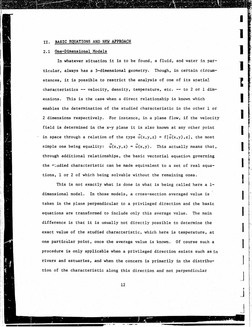
2.1 One-Dimensional Models

In whatever situation it is to be found, a fluid, and water in par-

ticular, always has a 3-dimensional geometry. Though, in certain circum-

stanc2s~ it is possible to restrict the analysis of one of its spatial

characteristics -- velocity, density, temperature, etc. to 2 or 1 dim-

ensions. This is th~ case when a direct relationship is known which

enables tha determination of the studied characteristic in the other l or

2 dimensions respectively. For instance, in a plane flow, if the velocity

field is determined in the x-y plane it is also known at any other point

~ ~

in space through a relation of the type u(x,y,z) = f[u(x,y),z], the most

simple one being equality: it'(x,y,z) = l:r(x,y). This actually means that,

through additional relationships, the basic vectorial equatio~ governing

the "':adied characteristic can be made equivalent to a set of real equa-

tions, 1 or 2 of whic.h being solvable without the remaining ones.

This is not exactly what is done in what is being called here a 1-

dimensional model. In those models, a cross-section averaged value is

taken in the plane perpendicular to a privileged direction and the basic

equations are transformed to include only this average value. The main

difference is that it is usually not directly possible to determine the

exact value of the studied characteristic, which here is temperature, at

one particular point, once the average value is known~ Of course such a

procedure is only applicable when a privileged direction exists such asin

riv.ers and estuaries. and when the concern is primarily in the distribu-

tion of the characteristic along this direction and not perpendicular

12

,.. • ' .• - • ;~·· ,.. • ~ ~ • • - -, • \ 4 • I ' ,, " . . ~

i I \• f'

I

"I

.I

'I ~~

. I

I I

I I

.I

'I

I I I I i I

I

J

.J l

CJ

J

'

l I 1 . i

' I. (·.

I I '_'~. I I I I I.

r 1 J

I, I 1 r ,·I i.

\

I I; ; j

'

I i: '.

I 1 I .J

I l ' I

' I; ! :

' I l I

1 ' ' i i

I I I

' I

I J' 1 '

t I. I

!

to it. In a stream the centerline is chosen as privileged direction.

One-dimensional models have the advantage of simplicity and they

require less data input than 2 or 3-dimensional models, particularly

where the boundary conditions are cuncerned. This is a very important

feature since, in mathematical models, one of the most difficult problems

is that of boundary conditions. The monitoring required for a 3-dimen-

sional water quality model of an estuary .muld be almost imposGj_ble to

meet, unless numerous simplification hypotheses are made which could des-

troy the supplementary precision given by a 3-dimensional study.

Moreover, where tramrver.se gradients are not too large, a cross-

section averaged value for BOD, DO, salinity or, in our case, temperature

is usually sufficient for decision-making in view of all the other factors

and unknowns which have to be taken into account. The hypothesis of a

small transverse gradient is not met when stratification occurs, as in

the vicinity of waste disposal devices, so that in those areas a 2 or 3-

dimensional near field study adds substantial knm~~·ledge to the tem-perature

or substance distribution. Though, in most cases, a relative cross~

sectional homogeneity is rapidly reached so that the zones where the

results of a !-dimensional model lack precision are very restricted.

Further justification for developing 1-dimensional models for water

quality lies in the fact that their range of application covers a substan-

tial part of the waste disposal sitns.

With the preceding remarks in mind, th.~ most general form of the

1-dimensional heat transfer equation for a variable area river or estuary

is as follows:

; I I 13

.;,: I ! ' I

.. • of\ • ~

' . .. . ... 1;1• J- . . ., ' . . . . '· -4 .

•'""" : -.., ,, ~"" ..-.:-wr-·- --~~--···••«a'~"'"'""'""""""'w_.w,. ><.,·,•""'"_"" __ ..._,.....,.,_~,..-"'---'•'-""'"'"1"'''-"''"~'t-"' ·''" ""'---~---"'"~--. . .

u !}

·-·---:--._=.J-· ---.··--.-..... ·--.• I ,., '

•

aat (ApcT) + a~ a ·=- [AE JL (peT)] + 0 b + WHD + THD L ax n (Qp cT) ax

(2-1)

where

A = cross-sectional area of river or estuary (ft2

)

T i d ( OF) = cross-sect on average water temperature

Q =

=

=

b =

X =

t =

pc =

discharge (cfs) of the river or estuary (including tidal flow)

longitudinal dis?ersion coefficient (ft2/sec)

net heat flux into water surface (BTU/ft2

.sec)

top width of river or estuary (ft)

longitudinal distance along the axis of the river or

estuary (ft}

time (sec.)

(density) (specific heat) = 62.4 BTU/ft3 . n:.•

WHD = waste heat discharge term (BTU/ft.sec)

THD = tributary heat discharge term (BTU/ft.sec)

The tributaries and waste heat discharges are considered as point

injections. The corresponding terms in Equation 2-1 are:

~1HD = i: Hi o(x-x.) (2-la) i

~

where

H. = heat discharge at injection point i (BTU/sec.) ~

xi = abscissa of injection point i (ft)

0 = Dirac delta function (dimension 1/length)

and

THD = I: Qj peT. o(x .... xj) (2-lb) j J

14

I

I 'I

:I ,,

I I

(~

I I :I 'I :1 I I I I I ,I

WI

: ,., f ~ ' "'\

1'

;;

I ,\I '. t·t

f1 ' t i

I 1

i

I/ I

j . , ! :;

1 l

1 j

I i

i'

I ~

< l

' '' I I

; 1

'i t!

1

t '

~

I :I ""!S'!:'-..

...... ~·"

>I~-

J •• 1" >I . • I I I I I I I I I I I I I

Where,

Q. = discharge of triburary j. (cfs) J

T. = water temperature of tributary J

X. = abscissa of tributary j. J

2.2 Net Surface Heat Flux: 0 n

(ft)

j. (oF)

Heat transfer ~etween a body of water and the environment can occur

through the free surface and through the bottom and sides. In the latter

case, the heat flux is limited by conduction in the adjacent soil and re-

mains very small because of the generally low thermal conductivity of

earth and because the temperature gradien~s are limited. Across the water

surface heat transfer by radiation, convection and evaporation is several

orders of magnitude higher and only these terms will be considered here.

Figure 2-1, taken from reference 2, shows schematically the more important

phenomena which contribute to the surface heat transfer. Not considered

here are the fluxes due to the heat contained in the evaporated water and

in the direct i_infall. Those te~ms are usually of much smaller magnitude

and can be neg!=cted. Though, the argument that they tend to cancel each

other is not fully valid, since evaporation and prec.1.pitation do not gen-

erally occur together and cancelation only happens in long-term averages.

Estimation of those various components has been the subject of many

theoretical and field studies and most of the derived equations are semi-

empirical. The following development is largely taken from reference 2,

where the current formulae are commented upon and new contributions have

been made to the determination of the heat flux in the case of an

15

" . . . . ~ . ~ . .. ' ~ ~

. 0 Clj. \

artificially he~ted water surface.

q,br

~s \

4>sr <Par

--Q

Figure 2-1. Heat Transfer Mechanisms at the Water Surface.

in which (units - energy/area.time)

cps =

=

=

=

=

=

=

=

incident solar radiation (shoi:t wave)

reflected solar radiation

net incident solar radiation = ~ - ~ '~'s '~'sr

incident atmospheric radiation (long wave)

reflected atmospheric radiation

net incident atmospheric radiation = ~ - ~ '~'a '~'ar

long wave radiation from the water surface

evaporative heat flux

conduction (sensible) heat flux

The units used in the following equations and formulae will be

stated as often as possible; they correspond to those currently used in

meteorology i.n the U.S., with all their incoherence. Fluxes will be

measured in BTU/ft2 .-day, temperatures in °F, pressures in millimeters

of mercury (mm. Hg), wind speeds in miles per hour (mph.) and heights in

meters. 16

.I I

1 1 I '1 1

I l I

I

I

t ,, I j; I

,f,

1: I ii ·t 1' ( ~

\l ,I: I

~ ~·

li

1! I.

I' I i

f I L I l l: ! l

I;

I 'l

I I I I I I I I

: l I i t l 1 '

I I

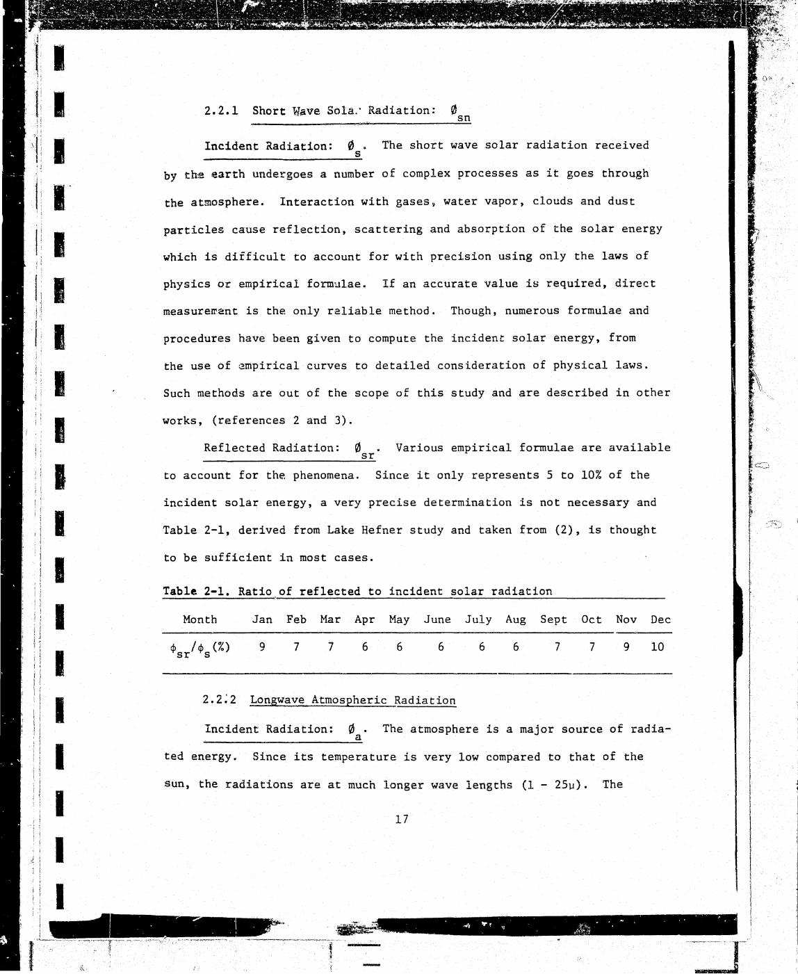
2. 2 .1 Short Wave Sola.· Radiation: 0 sn

Incident Radiation: 0 . The short wave solar radiation received s

by the earth undergoes a number of complex processes as it goes through

the atmosphere. Interaction with gases, water vapor, clouds and dust

particles cause reflection, scattering and absorption of the solar energy

which is difficult to account for with precision using only the laws of

physics or empirical formulae. If an accurate value is required, direct

measure~ant is the only reliable method. Though, numerous formulae and

procedures have been given to compute the incident solar energy, from

the use of ~mpirical curves to detailed consideration of physical laws.

Such methods are out of the scope of this study and are described in other

works, (references 2 and 3).

Reflected Radiation: 0 sr

Various empirical formulae are available

to account for the phenomena. Since it only represents 5 to 10% of the

incident solar energy, a very precise determination is not necessary and

Table 2-1, derived from Lake Hefner study and taken from (2), is thought

to be sufficient in most cases.

Table 2-1. Ratio of reflected to incident solar radiation

Month Jan Feb Mar Apr May June July Aug Sept Oct Nov Dec

¢ /q, (%) sr s 9 7 7 6 6 6 6 6 7 7 9 10

2.2;2 Longwave Atmospheric Radiation

Incident Radiation: 0 . The atmosphere is a major source of radia­a

ted energy. Since its temperature is very low compared to that of the

sun, the radiations are at much longer wave lengths (1- 25u). The

.( l .!

17

···=.s·

• I I

primary radiating element~ are water vapor, carbon dioxide and ozone.

Since the emission spectrum of the atmosphere as a whole is highly irre-

gular, the radiated flux can only be computed through empirical relation-

ships. Those usually deal with the atmospheric emissivity E which can a

be considered as an average emittance over the emission spectrum:

0 E

a (2-2) = a

a(T + 460) 4 a

where

0 :: atmospheric radiation flux a

0 = Stephan Bolzman constant = 0.1713 10-8 BTU/ft-2 hr-l °F-4

T = atmospheric temperature (oF) a

The influence of the clouds is usually accounted for separately,

so that the above formula is valid for clear sky radiation 0 ac Various

Si.apes have been given to E ac Some formulae only include t.t~ vapor

pressure as the one derived by Anderson (1954) from the Lake Hefner

studies:

where

E = 0.740 + 0.0065 e ac a

e = atmospheric vapor pressure (mm. Hg) a

(2-3)

Swinbank (1963) and Idso and Jackson (1969) have proposed formulae where

E is only a function of T . Stated directly in terms of radiation, ac . a

Swinbanks' formula is:

cpac = 1.2 l0-13 (T + 460) 6 a.

18

(2-4)

.L

.. .. I, ' '

I

I

I l I

I' j

Ll~ i;

~~ :~n-. !an

.,

j, I ! I

l I I

l i l I l '

1: I I

(

> i

I: i' l l ,j l ! I

=· ' I I

l <~

I I. I I·

and Idso and Jackson's is:

where

T a

= 4.15 10-S (T + 460) 4 [1 - .261 exp(-2.4 10-4

(T -32)2

] (2-5) a a

=

air tempe.rature at 2 m in °F 2

clear sky atmospheric radiation (BTU/ft -day)

Those two relationships give very similar values for tempera~ures

higher than 50°F but the last one gives better results below 4o•F. Though,

swinbank' s formula was us.ed in this study as the atmospheric temperatures

rarely went below 40°F.

Clouds tend to blacken the atmosphere thus increasing the radia-

tion. Their effects are accounted for by a formula of the type

= {2-6)

1Jhere

k = constant depending on the type, thickness and height

of the clouds

C = cloudiness ratio (0 for clear sky to 1 for overcast)

an average value of 0.17 is suggested for k.

~etlected Radiation: 0 ar A figure of 3% is usually accepted as

reflectan~. (or alberlo) for a water surface to longwave radiations~

0.03 0 a

Net Radiation! ~ an

(2-7)

Putting together the preceding results gives

19

- . ' i. • • .. . '<I~ • -

' .. • \ "' • • \ • '• • .,..1' .: L"J ~ _> ' . •

• • n • ~I •' • ,·"\ "";' • -p • .. .. . . ~- .... ~~-~.-.,-~--.. ~~-"''"'"'""~··-··

'lf -----

for the net long wave flux

1.16 10-13 (T + 460) 6 (1 + O.l7C2) a

2.2.3 Lcngwave Radiation from the Water Surface

{2-8)

This term is usually the largest of all the fluxes defined in

Figure 2-1. The emissivity of a water surface is known with good pre-

cision and this longwave back-radiation can be determined with accuracy

inasmuch as the water surface temperature is known precisely. This is

not always the CEde as a call layer usually forms near the surface which

is tt>o thin to allow a temperature measurement. But the following form-

ula gives a good enough approximation in view of all the errors intro-

duced in the detetmination of the other fluxes.

where

T = s

~br =

= -a + 460) 4 4.0 10 (T _ s

surface temperature in °F

back-radiation flux in BTU/ft2 .day.

2.2.4 Evaporative Flux

(2-9)

Evaporation from a water surface can occur as a result of both

forced convection (due to the wind) and free convection (due to the buoy-

ancy eff~cts). At natural water surface temperatures free convection is

negligible compared to forced convection. Though, when t.he water temp-

erature is increased, due to hea~; heat loads for instance, free con-

vection becomes sizable and has to be accounted for.

Many different approaches have been taken to determine the eva-

porative mass flux from a water surface. Most of the resulting semi-

20

I

J

" o 1 .. :... • t • .. -, t· ·1, \' r .. · • ._ t ~~ • • ....,.-:...-" ~ • 0 • ~ 1:1. .... • I . . : . . G

t r.

~I , I

~I r

.. ~

l I ;

t

I j I ~ . "l: r I ""' j"

1 : I lr

I: I I,

l ! 1·1 1 t

.111 I f

i -·

l{ I I I I I

! -·>1 I "' /f

l

L

I . I I I I

empirical formula can be written in the J::ollowing form:

where

w

E s pF(W ) (e - e ) z s z

E = evaporative mass

p = density of water

flux

= wind speed at height z

(2-10)

(mass/time.area)

z

F(W ) = wind speed function for mass flux including both free z

and forced convection effects (length/time.pressure)

e = saturated vapor pressure at the temperature of the s

e z

=

water surface

vapor pressure at height z

So that the evaporative heat flux is:

L E v

(2-11)

where L is the latent heat of vaporization. Within the range of tempera­v

tures encountere1 in the bodies of water under study, L can be taken as v

a constant and the heat flux becomes:

where

0 = f(W ) (e - e ) e z s z

(2-12)

f(W ) = wind speed function for heat flux (energy/area.time. z

pressure)

Natural or Unheated Water Surface: The number of formulae available to

evaluate f(W ) is great. A more detailed discussion of t:heir value is given z

21

' 0 ... ' • ,, " . ' I

• .... t • • ..- • I ·• - ..... •I .... Jlt- I

•• , >~;,.f • ' • ... I.,. '

't. . . . '

"I• ~ '-'

in reference 2, which conclusions we shall follow here, taking a refer-

ence height of 2 m and

(2-13)

where w2

is the wind speed at 2 m in miles per hour.

And

Artificially Hea_!:ed Water Surface. For a zer-o wind veloci, ty, mass

transfer by turbulent free convection can be accounted for by a diffu-

sive type equation:

E =

where

K ap

v m az (2-15)

E = mass flux of water vapor across the free surface

pv = vapor density

K = vapor eddy diffusivity m

z = altitude

If a simple analogy is made with turbulent free convection heat transfer

(flat plate analogy) Equation 2-15 can be transformed to yield

where·

0e = 22.4 (~e) 113 (e - e ) s a

~e ~ 'I - T s a

T = water surface temperature (°F} s

T = air temperature (°F) a

22

(2-16)

I

I

I I

I I

I:

j I ! :

l.

I I I I I I I I I

e a

atmospheric vapor pressure (mm Hg)

Theoretically Ta and ea should be measured at the same height.

Since water vapor is lighter than air, evaporation increases the

buoyant driving forces. This effect is taken care of by substituting

virtual temperatures for actual ones in Equation (2-16) which becomes

0 = 22.4 (~e )113

(e - e ) e v s a

(2-17)

where

.16 = T - T v sv av

and

T = (T + 460)/(1- 0.378 e /p) ~ s s

T = (T + 460)/(1 - 0.378 e /p) av a a

p = atmospheric pressure (mm Hg)

It would seem logical to account for forced convection as ~~s done

in the case of an unheated water surface by a factor 17 w2

(es- ea).

Though, experimental work performed by Ryan and aarleman (1973) seems to

prove that the predicted evaporation is too high and they advise a

coefficient of 14 instead of 17. Then for the heated water surface the

wind function is:

f(W2)

and

- 2L.4 (Ae )113 + 14 w2 v

(e - e ) s a

23

(2-18)

n ~ "' a ... ' • '" . , . . . • . • p . .

L 0

' ,. \ 0 (" .4Jik '" •l\' ' Q. ~ • Q ... ..

I. I

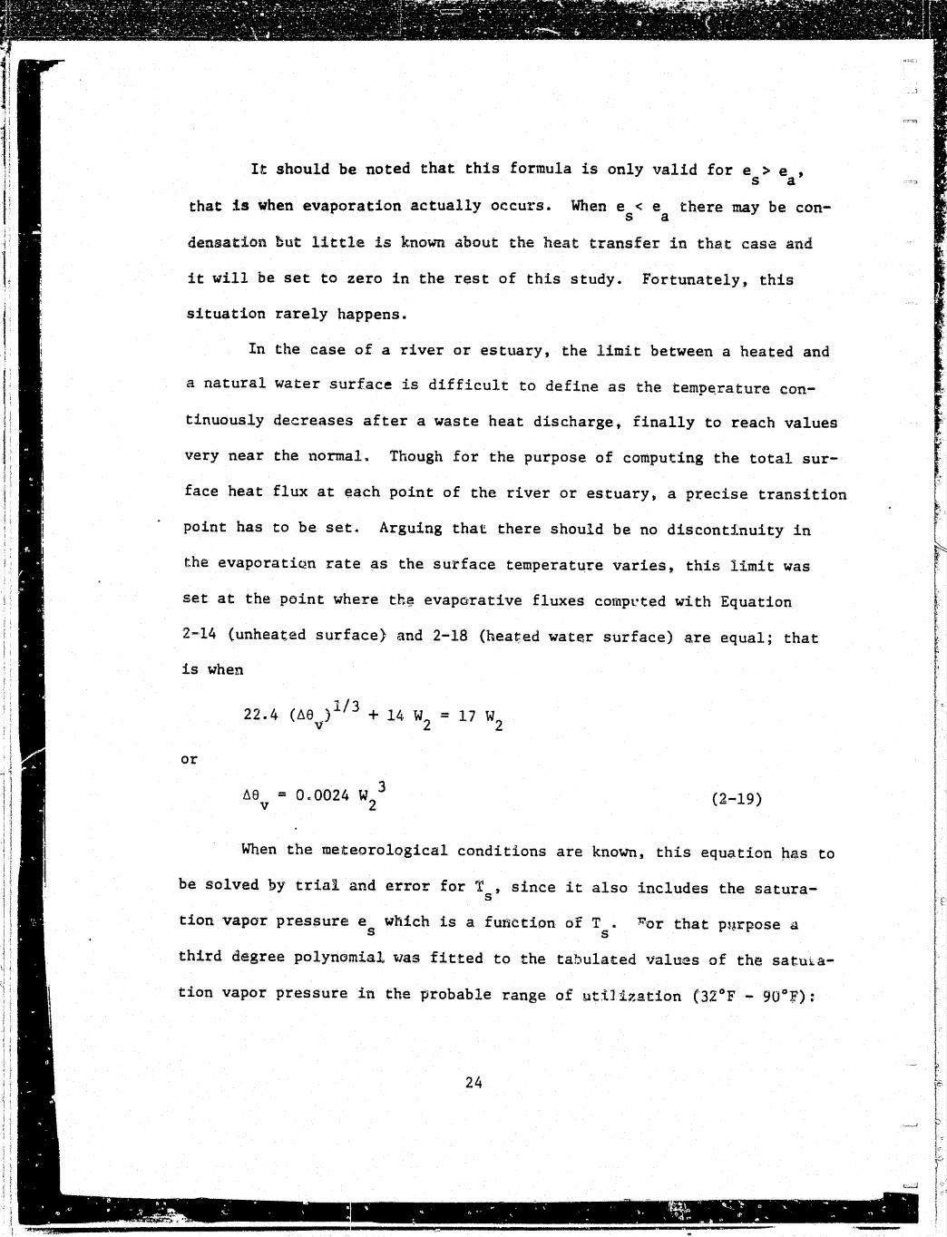
I·t should be noted that this formula is only valid for e > e , s a

that is when evaporation actually occurs. When e < e there may be con­s a

densation but little is known about the heat transfer in that case and

it will be set to zero in the rest of this study. Fortunately, this

situation rarely happens.

In the case of a river or estuary, the limit between a heated and

a natural water surface is difficult to define as the temp~rature con-

tinuously decreases after a waste heat discharge, finally to reach values

very near the normal. Though for the purpose of computing the total sur-

face heat flux at each point of the river or estuary, a precise transition

point has to be set. Arguing that there should be no discontinuity in

the evaporatiQn rate as the surface temperature varies, this limit was

set at the point where th? evapo,rative fluxes compt~ted with Equation

2-14 (unheated surface} and 2-18 (heared water surface) are equal; that

is when

22.4 (ll8 ' 113 + 14. w VJ 2 = 17 w2

or

ll8 3 (2-19) = o.oo24 w

2 v

When the meteorological conditions are known, this equ~tion has to

be solved by trial and error for 'l' , since it also includes the satura­s

tion vapor pressure es which is a function of T5

• r-"·or that p~}.rpose a

third degree polynomial. was fitted to the tabulated values of the sat:ut.a-

tion vapor pressure in the probable range of utilization (32°F- 90°f):

24

. . .. ,.. ~. - .. ~ . -...·. ,. ..,. ',• • • I ~ ~., Cl 1t. ._ ~ •

<q ,, • • .... ' t1" ... ..., , •• ' - • \ \ t"' -~ .. ""

! I

'' '

' I

l

! '

I I i

' I j

j

·tn

I tl I I I g

-

I ra-

:I I ' ~·,U ....

I I

e s

-2.4875 + 0.2907 T - 0.00445 T2

+ 0.0000663 r3 (2-20)

The maximum error introduced by this approximation is 5% at 32°F and 1%

A plot of the evap~rative heat flux versus temperature is given

on Figure 2-2 which shows the position of the transition point.

2.2.5 Conduction Heat Flux 0 c

Assuming that eddy diffusivity of heat and mass are identical,

Bowen (1926) related the conduction flux to the evaporation ·hrough a

ratio, now kr.own as the Bowen ratio R.

T - T s z

e - e s z

0 c

0 e R = = .255 (2-21)

the temperatures being expressed in °F and the vapor pressures in mm Hg.

The validity of this approach has often been put into doubt, but this

formula remains the most consistent with measurements.

2.2.6 Net Surface Heat Flux: 0 n

Gathering the results of the preceding pages gives a gen~ral

formula for the net surface heat flux.

0 c (2-22) - 0 + 0 sr a

0 ar

The determinat~on of the solar and atmospheric radiation terms

does not require the knowledge of the ~ater surface temperature and the

fluxes contributing to these terms will be grouped in a net radiation

term 0 . r

25

- ' ' • (\1\ ' . 0 • • . . ' ' \, . ~ "' . , ' - I . ' ._ • , . . • . ~ • , ..

"'"· ~ • • •• ' \ ~"' • : .... I) "' • \ • .. • \. • • • • • • \ . .. . • I t ~

./_

ftL~~-~~-~;··.::,:~:.·;t(::~·\:,:.}··::x?:'_;~L_-::'.~:'*_:::~=._.·-~:~-~~ ~~~:;.-.:~_-__ f_~c;::: __ ::~ ~: ~·-";~-.3 ~~·;)~:. ·. ~.~;;-----~l ~~-~·.'·-~--~~"}:~-'~----~;:. ~:---?}::~~-~-:~ -~~~:~;-]' ; ;

':1' •·.·. •.· :I . , \~........... ..

· ... : ''

17 w2 (e - e ) -s a

natural or unheated water surface

(e - e ) s a

22.4 {~6 )113 (e - e ) v s a

artificia}ly heated water surface

~-----------------------------*·------------------. T s

Figure 2-2. Evaporative heat flux versus surface temperature.

0 = 0 - 0 + 0 - 0 r s sr a ar

(2-23)

It should be noted that this net radiation term does not include the

longwave radiation from the water surface.

Then an expression for the net surface heat flux is:

0n a 0 - {4 10-8 (T8

+ 460)4 + f(W)[(e

8 -e) + .255(T -T )]J (2-24)

r a s a

26

. ' ' ' .a- '.

I:

I~

I

'I "I

I I I I I I

J

.J

f I j I i

l

I 1 !

I 1 :; ) .. ·~ 'I

I \ I

I E! )

I !:

j

I I

I I I I I

ll l \. I

1

I I

~~~t> ! }

I ~i 1

t

I '

' '

I i 1 > I

Following is a summary of the data requirements for the computa­

tion of the net surface heat flux. These data requirements can be divided

in two categories:

_ Meteorological conditions (MC) which can often be considered as .

constant over the length of the river or estuary under study, but which

are variable with time. They are:

T : a

r:

net radiation term 2 (BTU/ft .day)

b • (oF) am ~ent temperature

relative humidity = e /e a a sat

wind velocity at 2 m (mil~s per hour)

atmospheric pressure (rnm Hg)

- Water surface temperature T (°F) which varies with distance as s

well as with time.

For further use, the net surface heat flux will be written:

0n = 0 (MC,T ) n s

2.2.7 Equilibrium Temperature Concept

The equilibrium temperature TE is defined as ti:,e temperature at

which, given a set of meteorological conditions, the net surface heat flux

is equal to zero. It is a solution to the equation

(2-25)

and so, is only dependent on the meteorological conditions.

Reference 2 gives a way to solve this equation, using several

approximations, but the method still involves the assumption of a value

27

i I

. 'I • • • •

~ 0 • ' • • • Q • • .. • •

II f '. • • ' • , • ' • .. ~· ~~

for TE which is later checked and adjusted, so that it is believed here,

that a direct t~ial and error solution of .Equation 2-25 is the best way

to determine TE~ It is more precise and does not introduce more compli­

cation, especially when a computer is to be used.

2.2.8 Linearization of the Net Heat Flux Equation

For a given set of meteorological conditions, the typical shape of

the curve of the net surface heat flux versus temperature is shown on

Figure 2-3.

Considering the errors introduced in the determination of 0 , due n

to the utili?.ation of empirical formulae and to the space averaging of

the meteorological measurements, a linear approximation of the type

0 ~ - K (T - T ) n s E

(2-26)

can be considered as sufficient, particularly when the instantaneous

temperature distribution in the body of water under study does not pre-

sent a large difference between the maximum and the minimum. This is

usually the case in rivers and estuaries, in the natural state, but also,

to a lesser extent, when they are subject to waste heat loads as the

local temperature increases are now limited by law.

Though, if the approximation given Equation 2-26 is to be good,

the average surface temperature has to be taken into account in the

determination of K, as shown on Figure 2-3.

Here also, a method, involving a number of approxinations, is

described in reference 2 to determine K. This method requires the

28

. . .... ~' ~ .. . - .

,., "'']!

'

~1:. ·., I

~~~ . I L :

···)' . I

-l

I l

I :1 I

'!; . '~1 ! t

J, I I

r-· 1-1 ,, of

1.1 i

Ll I

I I I -I \I ! I l, 1

I I I I I I I

-K (T - T ) s E

Fisuze 2-3. Net surface heat flux versus tempet-atu't'e.

knowledge of the surface temperature and of the equilibrium temperature.

Since an. equation already exists (Equation 2-24) to determine 0 , the n

only interest of this linear approximation is its linearity with respect

to the surface temperature, which allows an easier solving of equations

involving 0 . T:1en, once an approximation of the surface tempjrature is n

!~nown, the easiest and most precise way to determine K is to compute 0 n

through Equation 2-24 and let K = - 0 I (T - TE). The units for K Ci-'!"~ n s 2 BTU/ft .day. 0 2'.

2.3 Transformation of the Heat Transfer Equation

Intrl.b.ttucing the linearized form 1:>f the surface heat flux into the

general form of the heat transfer Equation (2-1) gives

29

i. , ~ 0

" ' OJ -.... , ' I .. __...- .r, ~ o .. , • " ' I

' • I • , , 4 • • r • • ,..._ ' , ' ' ~' - I • • ~ ~ ~ •

' '

a a a a at (ApcT) + ai' (QpcT) ,. a;; [AEL a; (peT)] - b K (Ts TlO') + WHD+THD (2-27) 1-1

If there ie no vertical stratification, the surface temperature T is s

equal to the cross-section averaged temperature T. This is rarely true

but, when the average velocity is large enough to ensure good mixing,

the e~ror introduced by this approximation is small. Though, one must

always make sure that this approximation is valid before introducing it

into Equation 2-27. If this is the case, the number of unknown functions

is reduced to one in Equation 2-27 which, then, allows the determination

of the temperature distribution in the river or estuary under study,

provided appropriate initial and boundary conditions are furnished. It

is possible to determine the temperature distribution with or without

waste heat discharg~. from power plants by including or excluding the WRD

term. Let T(t,x) be the cross-section averaged temperature at time t and

abscissa x, with waste heat discharges, aud TN(t,x) the normal tempera­

ture, that is without waste heat discharge, at the same time and location.

Substituting in Equation 2-27 gi~es:

a~ (ApcT) +a~ (QpcT )= a~ [AE1 ;x (peT )]-b K(T) (T-TE) + WHD+THD (2-28)

where the dependence of the temperature on K is noted by writing K = K(T)4

This dependence will be studied in greater deL~ll in Chapter 3, bat if

T and TN are sufficiently close at all times and locations to allow the

30

r

I. I~

l I I I

J

I

l

' "'·

r II -~ 1

\

·l·l !

1-11) ·!

1• II

1

I I I

11 . n

\

i 1 !

' . '

t'

t; I'

' ! ; j: : l

l

I ) I

on.

I

I !-29)

I :r).

I !

I I I

K(T) = J{(TN), Equations 2-27 ..._";~d ~-28 can be subtr.::;cted to approximation

yield

AT = T-'i' is the temperature excess over the normal due to the where u N N

h t dic·charge This value is interesting as it can be considered waste ea ·' ·

a measure of the thermal pollution.

Equation 2-30 is very similar to the BOD mass transport equation:

a (AL) + JL (QL) = JL [AE aL ] - K1AL + Discharges ;w ax ax L ax

(2-31)

where

L = BOD concentration

= BOD decay coefficient (dimension: 1/time)

th~Jgh major differences exist:

a) In the BOD case, the decay is proporLional to the amount of

BOD present in a control volume, which gives the term -K1AL in Equation

2-31; whereas in the temperature case, the heat loss is proportional to

the free surface area of the considered body of water, which gives the

term -K b 6T in Equation 2-30.

b) In the BOD case, the decay coefficient K1 can be considered

as constant:; whei'~as for the temperature it varies with time, since it

ls dependent on the meteorological conditions; and with distance, since

:lt is d-ependent on the surface temperature. The dependence on the time

i.s very important since this equation treats unsteady flow!: and since

31

•• \ Q • - ~ • • •

• "' I>. - .., .. .(1} ' • "" ~ '

• fl.1 ,_ -'-"l I • !'- o, ~ • ~ IJ • , • -

i

1 i

l I I. t :

I.

I j!

the relative amplitude of the variations are large, as between day and

night. For instance, in extreme tidal flow cases, where the amplitude

of the tide is of the same order of magnit·ude as the mean water depth,

the temperature difference betlli~en tw~.... low water slacks cat be as high

as l0°F accordirj to the time of the day. Taking a constant K would

suppress those differences which can be very significant to the aquatic

life.

c) The knowledge of ~TN is usually insufficie~t when an assessment

is to be made regarding the impact on the ecology and it does not allow

any verification of the model since the temperature excess canna= be

determined by measu~emenr.

This shows that temperature cannot be treated exactly as BOD and

the model described in Reference 1, where Equation 2-31 is solved, has

to be modified to account for those differ~nces. Equation 2-1 will be

solved directly, computing 0 from Equation 2-24, since the introduction n

of the linearized form ~[ the surface heat flux loses much of its inter-

est when both K and TE are variable.

A full discussion of this approach is given in Chapter 4, but

before that, a steady model will be considered which allows a better

understanding of some of the phenomena involved.

32

, •. I~

I

I~

I I I I I I I I I I .I J

·41

1: ~ ;

il ;(

I; ' i

I , I I

I I

).

I l' ! :

I.

i I ..

i: :

'l

I

~~ I

l ~ I

I I I I I I I I I I I I I I I I I I I

III. STEADY STATE MODEL

3.1 !!X£otheses

In this simplified model the hypothesis is made of a steady situa-

tion for the meteorological conditions as well as for the river discharge.

A steady river discharge implies constant velocities and cross-sectional

areas with time, as can be seen from the continuity and momentum equations

which govern the flow. Though, the cross-sectional area is allowed to

vary with distance.

3.2 Possible Applications

Although steady state conditions are never met strictly since the

river discharge varies along the year, and so do the meteorological con-

ditions, this model has the advantage of simplicity and can be applied

in many cases as a f1.rst approximation by taking average conditions over

a limited period of time a month for instance.

Moreover? this model determines the temperature and not the temp-

~rature excess as many which are derived from Equation 2-30. This allows

much ~asier verifications and eventually adjustments over the average

conditions chosen.

We saw in Chapter 2 tha1; the heat decay coefficient varies with

the surface temperature as well as with the meteorological conditions.

In this steady state model, since the m~teorological conditions are held

constant and since the surface heat flux is computed directly from

Equation 2-24, exact values oi' the ciecay coefficient can be obtained.

and the influence of the surface temperature on it, can be explored

In this model, as well as in the~ unsteady one described in Chap-

ter 4, the meteorological conditions at:e covsidered as constant over the

33

~ . , . . . ,, . ' . I . . ' . • . ~ ' • • • D ; .. ~ • • •• • ~ • ' • II • - • "

.. . "' ....

"' I i ~ I

~

I: ' '

i ~~

'

l:

l I i '\

l.

. 'i <

; ;

.. l 1'

' ''

l

whole length of the river or estuary under study. The degree of exacti-

tude of this approximation depends on the length considered, but, in any

case, some errors arf! introduced. Moreover, since a continuous record

of the required meteorological parameters is rarely available., time-

averaged values over periods of 1 to 3 hours or more will be used in the

unsteady model. Supplementary errors are introduced by this procedure.

In order to obtain an idea of the subsequent errors in the temperature

distribution a sensitivity analysis will be performed in which a c.orrela-

tion coefficient will be computed between each of the meteorological

parameters and a representative characteristic of the temperature dis-

· tribution.

3.3 DeveloEment of the Model

Under the assumptions stated in 3-1 the general one-dimensional

heat transfer squat ion

a (ApcT) + .1... (QpcT) = _a at ax

(3-1)

becomes, for steady state conditions,

a a a ax (QpcT) ~·ax [AEL ax (peT)] + b 0n (3-2)

For a river, the dispersive term can be neglected and in a zone

where there is no tributary, aQ/ax = 0. Within the range of variation of

the temperature the term pc can be assumed to be constant and the final

form of the equation is:

dT -:11:

dx

0n(T) b(x) pcQ

(3-4)

34

fl I I I. ~-

I I I I I I

f

I r l I

l 1: r-

jc

I n IJ

~ I I

I !'

I I l

l. ,~

l

I I I

i' t

f l I .,) ~

l I l• j'

I I •' I

r I I' I ~ 1 1 ~ i

I I !

' I; j l

I I: I I I I I I fl

I I

'I !

:

I

This first order ordinary differential equation can be solved if

one boundary condition is prescribed. The easiest way to do it, both in

the field and for the model, is to specify the temperature at the upstream

end of the river portion under study.

T = T 0

at X = X 0

(3-5)

Discontinuities appear if there are tributaries or waste heat discharges.

At those points dT/dx is no longer defined and there is a change in the

discharge Q so that Equation 3-3 is not valid and a new upstream boundary

cohdition should be specified.

If at x = xA there is a •;ributary with a discharge QA and an

averagt~ temperature T L the new discharge will be Q + QA and the new up-·

strea~,l boundary condition

T = at (3-6a)

If the discontinuity is due to a waste heat input: of H BTU/sec.,

there will be no change in the discharge since the inplant water losses

are usually small compared to the river discharge and the new upstream

boundary condition will be:

T =

Simplified Case

+ H pcQ at (3-6b)

If the width b is constant and if the surface heat loss coefficient

K is assumed to be independent of the river temperature, that is, if we

take

35

. ~ . ' . . . . ' \ . . .. -.... \ " • 0

. "' ~ . . . . - ,.).. \ • -.. • • • 0 .._ f:l • I

(3-7)

Equatton 3-4 beco~es

dT Kb (T - T ) (3-8}

= --dx pcQ E

and an analytical solution is easily found to be

b K -~)x

T = T + (T - T ) pcQ (3-9) e

E 0 E

General Case (varying width)

In the general cas~ a finite difference scheme was used to solve

Equation 3-4. For that purpose a one-dimensional partition of the rive~

is done:

• .. ft • 0 • , X }

n

with segments [xi' xi+l] of non-necessa~ily constant length to allow

a smaller mesh spacing in the zones where the temperature gradients are

larger.

If T.1

is the cross-3ection aver~r·-1 temperature at abscissa xi'

we have according to the Taylor formula

substituting in Equation 3-4 gives

Ti+l - Ti

xi+l - xi =

0n[T(E:i)] b(t;i)

pcQ

36

(3-10)

(3-11)

I, ~ ~

(;)

fl

'~

I { ) 1 .

"

l

t

'j

'l f; : : ! :

, , r

\ ~ J

' l

Since the temperat.ure?, distributiop usually has an exponential

shape, ~i is more in the middle of the segment [x1 , xi+l] than at one

extremity, as shown on F'igure 3-le So, th~ value of the width will be

taken at

and, in order to simplify the geon1etrical data input, a linear interpola-

tion will be performed between xi and xi+l,

T

Figure 3-1.

distance

Position of ~i in the interval [x , x ]. i i+l

31

Cl-12)

.. \ . ·<· ... ..:0. ~~ ~ • • {\ • • • • • • • \ • - , . • " " - ::- • ~ • j •

_. • " • ' \, "' I ' JV ' j t~ 1 .J I ,}

f

r j

'

I

Such a procedure cannot be applied for 0n[I(~1)1 since the tempera­

ture at xi+l is unknown and the functional relationship ll~tween 0n and T

So 0 will be apprmtimated ~t the n prevents an implicit determination.

preceding mesh point xi. It is important to determine if such an approxi­

mation will not engender cascade errors as the numerical computations pro-

pagate. Let us consider the simplified case of a constant width. The

compute!d temperature at abscissa xi being ! 1 and the real one T:l. we have: -

'I + (x1

- x ) 0 0

0 (T ) b n o

pcQ

(3-13)

------------~------------------

suniming up give.s

(x. -x. 1) 0 (Ti 1)] 1. 1.- n -·

(3-14)

writing similcr equations for the exact temperature would give

so that

T -T =.JL i i pcQ

(3-16)

38

f ' .

. . . "'- . . . . . . . .

' ~ . . ' I I'

'' ,•

'

' j i:

:I

i ;

; i ( . 'j

1 I i l

.-1>]

3)

I r· .. ~. , ..... ~T:"'~-:~- ·;.- '·

Let us suppose that from k : 0 to i~ Tk - Tk has a constant sign.

If. to begin with, T0

> TE' T(x) will be a decreasing function and

T > T(E; ) 0 0

" (T) is a aecreasir.g function since w.rn '"'

0 (T ) < 0 [T(t )j n o n o

x0

) [0 (T )- 0 [T(t )]] < 0 n o n o (3-17)

and

Figure 3-2 shows how the solution is approximated in this case, when

T - T keeps negative.

T Q

Ti-l T - i Tk+l

Ti-l

X xl x2 xk xk+l xi-1 xi 0

Figure 3-2. Approxfmati~n of the solution in the most unfavorable ease

39

1 ' i ...;,

'~

r ..

,.,

...J

·'

'"-'

~·

'"" . ~J

t { j

·-~

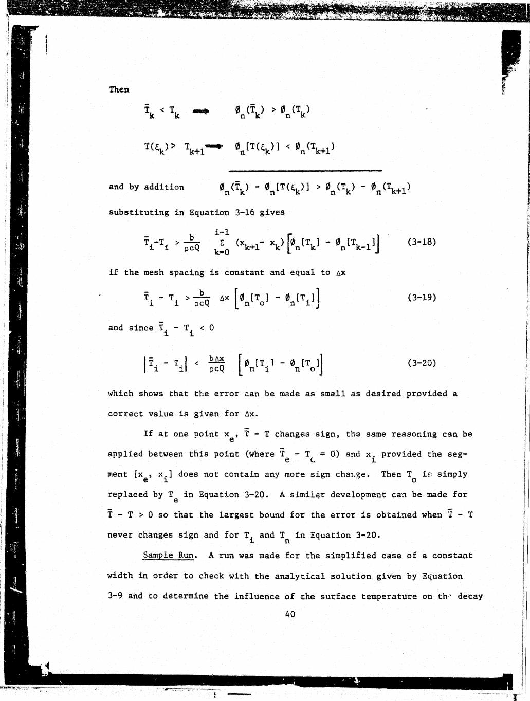
Then

and by addition

substituting in Equation 3-16 gives

b >-

pcQ

if the mesh spacing is constant and equal to ~x

-and since T. - T < 0 ~ i

bnx pcQ [ 0 [ T • 1 - 0 [ T ]]

n 1 n o

(3-18)

(3-19)

(3-20)

which shows that the error can be made as small as desired provided a

correct value is given for ~x.

-If at one point x , T - T changes signt the same reasoning can be e

applied between this point (where 'r - T = 0) and x. provided the seg-e {. ~

ment [x , x.] does not contain any more sign cha1;:c;;e. Then T i!li simply e ~ ,, o

replaced by T in Equation 3-20. A slmilqr development can be made for e

-T - T > 0 so that the largest bound for the error is obtained when T - T

never changes sign and for Ti and Tn in Equation 3-20.

Sample Run. A run was made for the simplified case of a constant

width in order to check with the analytical solution given by Equation

3-9 and to determine the influence of the surface temperature on th;· decay

40

I I i , I ; (

I. I

l'

\'

''

1 ;

I i; l ~

; I 1 1

i I

I I,

! l ·

1 be i; I 1

I •-r : , '1

i ; .y

! : Jr { ~

'' I

. ! - T

' \: I I'

'.1

n '

" !

: 'deca.y

'' I

._::;; >

J ' I '

'

coefficient K. Exact values of K were determined at each step by divid-

surface flux computed with Equation 2-24 by (T- TE). ing the net

is determined at the beginr:ng of each run for the corresponding meteor­

ological conditions by trial and error. This influenc • of the temperature

on K is particularly important in the derivation of Equation 2-29 where

K is taken to be the same with and without waste heat discharge. This

was explored by introducing a 400,000 BTU/sec heat input at x = 0, which

gives a typical temperature excess over the normal of 6.5°F at the injec-

tion point, with the 1000 cfs river discharge chosen~

£he geometrical and meteorological data for the sample run is

printed at the beginning of the results outputs given in Tables 3-1 and

3-2. The resulting temperature distributions, with and without waste

heat discharge are shown o~ Figure 3-3.

A 50 ft. mesh spacing was chosen {although the results are given

every 500 ft.) so that, with the waste discharge, where the temperature

variation is the largest, and so the error, the maximum error for the

47,000 ft. under study is less than

bnQx [0 (55.'}8) - 0 (61.41)] ·- o.oos pc n n .

as given by Equation 3-20. Working with the program has shown that the

error is usually much smaller (up to 5 times) but this formula has the

interest of giving an upper limit which is a measure of the model pre-

cision and can be used as a discretization criteria when a value of the

maximum temperature variation can be esti.mated beforehand.

It appears from the runs (see following pages) that the surface

41

. . . . . . . . . .. . : . . .. . . . :· . \ . . ~ ' . . : . . . . . . .. . ....- . . ' . ____________ ....__ ______ ~·-·- '< ,..,..-:--. -... -::--1 -

-

f

' '

] .. ,. l

I ! :

''

i' f: ; !

i:

TEMPERATURt: DI~TRI~UTION ~TLil>Y ***$***********•***********•**

THE ~MhlANT TEMPEPATUPE l~ THE PELATIVE HUMIDITY I~ THE '..liND VELOCITY AT 2M IS THE NET RADIATED FLUX IS TH£ ATI.,O~PHEP!C PnESSUR~ I~

EQUILIHRIUI•l TEMPERATUPE

60 OEG r • 7?

1 e 111/HOU P 250~ UTU/FT2/DAY

760 i~"IM H G

52.7969 PEG. F

THE PIVER Dl~CH~PGE I~ Hl0fi CF~

THE HEAT DISCHAPGE 1~ " f\ Tll/~

THE ItJl TIAL TEi1Pl:: r.~TU rE OF THE PIVEP lt:" 55 DEG F

rTATlON (ft) '.HDTH (ft) TEnPEPATUPE <•r) DECAY (Bro/•r.a.ft2

)

-r. 1C0~ 55

+"' 10~0 55

50U H>k)0 54.9734 1.51948£-~3

1 er.0 10~W 54.947 1.51914E-e3

150~ HHl~ 54.921 1.51R79E-03

2r'~" 1"ee 511.895/i t.:·1845E-03

25~0 HHW 54.£7 1 • 5 1 8 l 1 E- 03

3~0r: 1C00 54.8115 1.51776E-03

35t:l0 HW0 '511.82"'2 l .51745£-~.3

4"-lkl~ Hl0U 54.7958 1 .5 1711 E- 0.3

4~k>0 1~~" 54.1717 1.51678£-0.3

5~~~ l~k10 5Lt.7478 1 • 5 16 4 BE- ~: 3

55UIC 1U~0 ~4.72113 1.?\616£-03

GfOk'>fO liH1~ 54 .. 701 1 .515R5E-03

6~~k'J 1 ~)k'·~ 54.6781 1.51553[-03

7H~.~ki ·~"'~ 54.6554 1 .5 15 ?.4E- 03

15 Uld 1000 54.633 1 • 5 14 93 E .. 0.3

i:.Wki~ 1 '''-'(£) 54.6108 1 • 5 14 6 5 E- ~.3

850~ HJ~~ 5.4.589 1.514.36E-03

9~fc.10 ~~"" 54.5674 1.51406E-03

95mi tum: 54.54€; t.51377E-~3

1 ~HJ1r10 ll~l'lr1 5~ .5~5 1.5t351E·0~

1050k> 11:\00 54 .se4 1 1.5t3~2E-e,

11000 U~00 5LI.4S3 6 1.51293E-~3

11 5ft1L1 10~0 51~ ,.4633 1 .5126BE- 03

12.k'0~ 1 ~0,1 54.411.32 1.51?.40£-03

1 ~~500 1"00 5'1.423 4 1 • 5 12 1 4 E- 03

13000 ~'"~0 54.4038 t.51187E-03

13500 1"01£) 54.38.05 1 .5 1161 E- ~3

14~~0 1 '"'0 54.3654 1 .51137£-~3

14500 1000 54.3~65 1.51111E-2'3

15 "00 100~ 54.3279 1 .5l~B6E-~3

155016 1000 54.3095 1 • 5 10 6 l E- 0.3

16U01r1 1000 54.?.913 t • 5 103 7 E- 03

16500 1000 54 .fn33 1 • 5 10 1 4 E- 03

17000 HH10 54.2556 1 .. 50990£-03

17501r1 HH:10 54.238 t.50965E ... 0~

1 fHH:l0 !000 54.2207 1.50942E-03

Table 3-1. Reproduction of the computer output for the steady model

sample run without heat discharge. 42

l_)

,, \

!' l

I j

J ~""TiiTI OtJ (ft) WIDTH (ft) TEf-1Pl::f!ATU~"E (•F) lJl::Ct.Y (ITUrF.n.ft2) J

Hlt:U 54.~036 1.5~9~~E-e3 1 65~1" 19iH~Ii) HW~ 51!.186 7 J .50896£-03

195~H! U1"kl :,4.17 1.5087i!I::-03

:~ ~~kl"k111.l 1 k'" 0 5'• .. 15.35 1 .. 5~853£·03

Zt15k.l01 i~k'" 54.137~ 1.50830 E-V.3

~! 1 "~~ HHH.; 54.1211 ! .50809£-03 ·~

215~~ IU£10 5'' .105 2 1 "50788E•£3 '~ ~~D ~k>" 1"00 51r.(i895 1 •• 5e767E-03

2250~ t000 54.C74 1 .. 507 46E- 03 ~.

23"00 10"" 54.~5Fi7 1 .50727£-03 t I

235t10 1 ""0 54.~436 1.50704[-~3 J 24000 10,HJ 54.~286 1.506RfE··~3 ~ 24500 1 'HH;) 54.~H38 1 • 5 06 6 7 E -IZ 3 ~1\l

t 25000 HHH> 53.9993 L.SC646E-03 ;

I : £5500 100" 53.9848 t.se~29E·03 ! ! ;., ' f

Z6000 1000 53.9706 1.50609£-03 ~~65~0 HH:~0 53.9565 1.~;0587£ .... 03

1 \

27ii00 HJ0~ 53.9426 1.~SiJ569E-el3 ,

27500 HH:HJ 53.9289 1.50553E-03 ' .t 1 ~800~

1 ""'"' 53.9153 1 .• 50532E- 03

L,>

285~0 10Nl 53.9019 1 .505 J 6£-03 290kH1 HW0 53.FiJ:!R7 1 • .SC4~8E-IZ3 295"0 10~H1 53.E756 1 .50480£-03 30"~" 1000 53.8627 1 .50463E-03 ~·· 30500 100~ 53 .. 8499 1.50445£-03 31000 1000 53.8373 1 .5042~E- e3 . ' 3150~ 1000 53.8249 1 .5 r4 e9E- 03 32~00 1~0U 53 .. 8126 1.50393E-03 ~,A 4

325~0 UW0 53.80"4 1 .5fl13 77E·· 03 33000. 1000 53.7884 1.50,'Hi0E•03 ' l

3350~. I 000 53.,7765 1.50345E-03 340~0. 1~00 5~,.7648 1 • 5 0329£- (13 .,

L .. l

345"0· 1~00 53.7~32 1.50313£-03 ~ 35 0160. 1U00 53.7418 1 .5~l298E-03 ,, '

355~0. lldlH' 53.7305 1.502SJE-03 36(1~~. !U00 53.7193 1.50269E-e3

--~ 365016. l0C(1 ?3.7083 1.5"'252£-03 3 70~Hi .. 1(100 53.6974 1 .5023 7E- 03 375~~ .. HH:l0 53.6866 l .50221 E- 03

. l 380'>0 • 101"0 53.676 1 .502l18E-03 3S50k>. 10~0 53.6654 I.5kit93E-e3 39t!e0. 1UU0 53.6551 1.5Ul79S-03 39500. 1 ~00 5.3.6448 1.50167E-03 40e00. l0UC 53.6347 1.5~H 49E-03

i l 4050~ .. 1000 53.62LJ6 1.50136E•03

' ! 4Hl0"· 1r;,00 5.3.6148 1.50122E-~3 4151616. l00kl 53.605 1.501URE-t'3 4200~. 10~e 53.595 3 1 .5 0096E- 03 4}~5t 16. HJ00 53 .. 5858 1.50~R.3E·(1~

i' i' 43~00"' lb00 53.57~ 1.5006RE ... 03 I' 435ll0. 100~) 53 .s6·· 1.5r056E-03

'' 44,H)i0. HHJI6 53.5579 1.5~f'46E·03

) 44!HHl. HHHi 53 .:·4P8 t.50e3eE .. 03 '"·' I 45000. HHHI 53.5.398 t.5"r.t7E-r3 I. 45500. 1 0~HJ 53.53C9 1.500"7£ ... 03

460~~1 .. 1000 53.5 ~!~!~ 1.49994E-C3 46~'-.;il. Hl00 53.5135 1 .1499 R3 E- ~·3 IJ70li0. 1 "'-! ~~ 53 .5,14!) l ·'19973£-03 ~ll·

., . . ... 43 Yo

-~ I

-I • • ' ~ \_. ....(1 • ••• ' •

"( ~ • 1

41\; '\ • l I .,..,. '

' ' '

I

TE!JPERATUP.E DI!1Tr.I£lUT10ti c;TUUY ****************************~*

UY L!UiEC! CALCULATIO~~ OF THE SUT?FACE HEAT FLUX

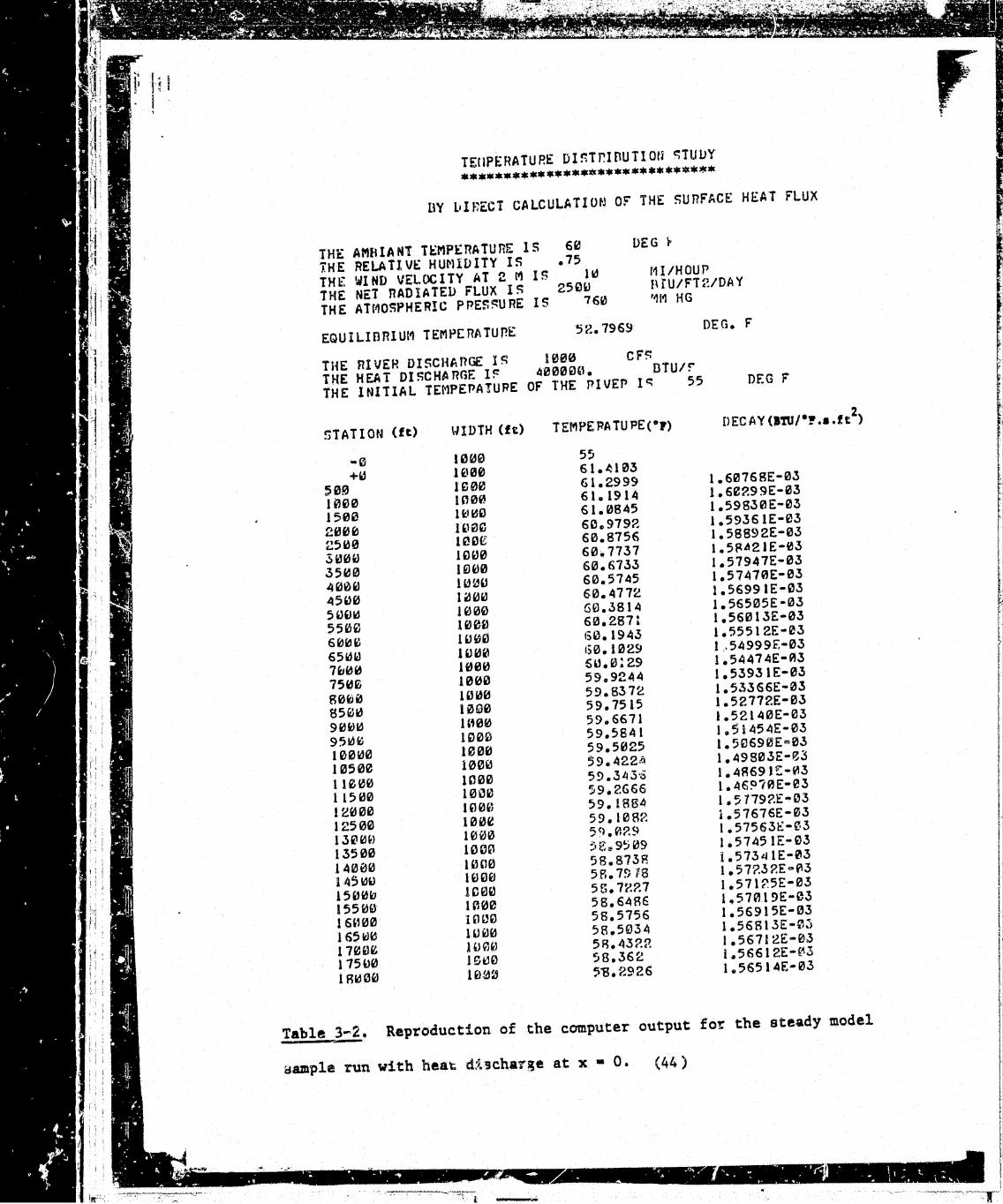
I>E G f. THE AMHlANT TJ::MPERATURE lS 1.HE RELATlVl:: HUNllJITY 15 TH£ WIND VELOCITY AT 2 M 15 THE NE1 RADlATEU FLUX IS THE ATM05PHER!C PPES~URE IS

60 .75

lid 250~

760

f11/HOUP f\ ru/FT2/DAY '11'1 HG

EQUILIBRIUM TEMPERATUrE 5?.. 7969

THE RIVER OI5CHARGE IS 1000 CF!'-: THE HEAT DISCHARGE 1~ 4000tni. DTU/r THE INITIAL TEMPEPA!UPE OF THE PIVEr I~ 55

STATION (ft) WIDTH (ft) TEMPE~ATU PE("l)

•0 1000 55

+" 1 t.l00 61. ~10.3

:; 0!'J lS00 61.2999

1000 1000 61.1914

1500 1 ~1l1'l 61.0845

2000 HH'S 60 .. 979?.

2500 UHH:: 60.8756

.300" HH'0 60.7737

3500 10~0 60.6733

400~ ·~~" 60.5745

45"0 li100 60.4772

5 "tH6 1000 60.3814

5500 1000 60.287:

600~ 1"~0 60.1943

651dld Hl00 150.1029

7iJ00 1000 su.0;29

750E 1000 59.9244

80~0 UH60 59. 8.3 72

as~1.1 HHl0 59.7515

90~1.1 H'00 59 .. 6671

9510ki 1000 59.5841

100160 1000 59.5025

10500 1000 59.4224

11000 lC00 59.34.3'6

i 1500 10"0 59.2666

12000 Hl0'~ 59.1884

12500 100£ 59. 10 8~~

1300~) HHJ0 5'=). ~?.9

1.3500 1000 !d.<;.,.9509

.14000 UHl0 58.873R

145 1.1k> HHlfJ 5P,. 79 H3

1500" HHJ0 55.7?.?.7

15500 1~00 58.64R€ 16,,00 Hl00 58.5756

165kl~ HH.I0 58.5034

1700~ HH1~) 5R.43?.g 175~0 10t10 58.362

1RI.10~ H.l!d~ 513.2926

DEG. F

DEG F'

1.60768£-03 1. 6e?.9 9E-03 1.59830£-03 1.59361£-03 1. 58892£-03 1 .. 5~-421£-03 1.57947£-03 1.57470£-03 1.56991£-0.3 1.56505£·03 1.56013E·03 1.55512£-03 1 ,• 54999£-03 1.54474E-A3 l.53931E-03 1. 53366£-03 1.52772£-03 1.52140£-03 1. 51454£-03 1.5~690£e03 1. 49803£-e:i 1.4H69lE-~3 1. 46?70E·03 1. 5779?.E-03 1.57676£-~3 1.575631-.:-~3 1.57451E·03 l.573lllE·03 1.57?,3?,£of'3 1.571~5£-03 1.57019E-C3 1.56915£-0.3 1.56813£-0:; 1.56712E-03 i • 5 6 6 1 2E .. f'\ 3 1.56514E·03

!!ble l:£· Reproduction of the computer output fo~ the steady model

aample run with hea'G d3.Jcharge at x • 0. (44)

I' I l

:

I~ 1.

\''

1

j:

:;

1 i

l : l !

' 1 i i! ! I

' !

! ; i

j I I'

~"TI\TION (ft) Hll>TH (ft)

185~k> HHHI l ~!1'11rJ 1 ~)(ll~tJ HJU~ 1 ~)50(!;

~!~~0k1 Hlw}~

?.~~t;0 HJ0{1J

~~HHl~ Hi0V. ~! 1500 1000 22000 1 k; 0") 2~!511~ } ,1~0

23~H!J~ lll~~i

23500 1~00

?.4~00 1~>00

24500 lVHi~'

:!5tH'" 1000 ~!55C0 I00P t6hH: HHJ0 265tJ~ HHH.i 27'->00 HH1~

~~ ?,~j~, Hl~0 ?.fH: t1e 1 ti ""-' ~851Jki HHJ~

29'-~~ 1':~.w ~:95 l:Jf(J HHH.I

3 '~'H:l0 HHH! 3050k3 1U0C 3H.'G0 HH'0 315C~ l ",,~ 32000 1C1Z~

3 ~!5 ,~(0 H.W~ 33C:HHI. 1 ~ li': 33500 ~ 1 £!'· k30 34"~c. HH?C 345~~. ll10~1

350Qf(J. Hw~: 3550~. HH.1~

3 6~HH:1. Hi~~

3650ltJ. l~U~

~~ 7000. H1 "~: 3 751tJft 0 1000 38e00. 1000 3·851cHJ. 100~ 390~0. UHHI 39500. Hl0C 40000. lltJ~O 40500. l~U~

4100~. 1"[10 4l50k3. HHl" 420~H.i. H1"'~ 42!i00. 1~00 ~300~. HW0 4350~. 1 "00 /f '1"00. 1000 4450~. 1 '! U0 1!5ll~0. 10"~ 4.550~. UW0 4 61a~~0 ~ 100~ 46500. )00{1

4 ":00. 1 "or.

45

~---" "'~r----.-.·~""--:"·-

f' •I ';

' -! .... + ~ .. ....,.

T iftlJl £ !> '' T U rE:

~~.224~~ 5H.l566 5H.U9 ~ ~. ~~!4~! 57 9 9593 57~8952 57.8319 57.7695 57.7fJ79 57.647 ~7.587 57.,5278 57.4693 57.4116 57.35115 57.2983 57 • ~:Lt27 57.1879 57.13.37 57.~8C.~ ~ 7. ~~~ 75 56.975il 5€.9?.4 56. 873~! 56.8~31 56.7736 56.724?. 5€.G76G 56. 6~!89 ~6.5819 S.G.5355 ~· 6.11897 56.4''''" 56.39~8 56.3556 56.3121 56.2691 56. ~~:~66 ~6.1847 ~(!. 1433 56.1"?.4 56.0€2 56.m:!22 55.9828 5~. 91:4 55.9056 55·.8677 55.83 ?.3 55.7933 55.,7568 55·. 72~8 55.6fl:52 55 .. 65 55.6153 55.5811 55.5472 55.5138 55.11f~"8

.. rt .I I

<•r) ll£Ct, Y (l'l'Uf0f.a.tt2) j

1.56417£-03 ' 'I 1.56.32JE-f3 I

1.56!:~7£-03 ,,

1. 56I34t:-;? .. ~ 1.5>S043E-03 1. 559531!:-03 }

1.55864£ .. ~l3 I 1 ~55 717E-tJ3 1. 55 690£ .. 0.3

c~

r.,~

I.556esE-e3 ' l 1.555!:1£-03 .J 1.5543RE-V'3 I 1.55356E .. ,'3 t .. 55276E-e3

r-.:$,

1.55197£-03

·-1.5511E!E-03 1 .. 55~,41£-03 le 5Lt965!::-f13 f

1.54890C:-f3 !, . j

1.5LI815E·€3

·~ I. 54 743E-03 1.54671E-P3 t.54599£-r3 l I. 5''53eF.-03 1. 541161 E-f-·3

'-t .. 5439~E-r3 1.54325E-03 1 • 54 ~5 9 E- vi 3

• 1 .. 54193£-03 1.,51l12RE-03 1.51l065E-,43 1.54~r.2E-03 !

, ... :t

1. 53940E·03 t:;

1.53878£-03 l -.)

I. 5381 CE-C3 1.53759E·e'3 ~ • 1. 53 70i'E-£3 11.153642£-03 1.535851::-0.3 1.53529E-03 1. 534731::- t'3 t.534ISE-e3 1.53363£-~3 1.53310E-C3 1. 5325 RE-03 J.53205E-03 1 • 53 15 .4E- 03 l.53I03E .. e3 1. 53053E-03 1. 53~r. 4E-rt.; 1 • 5295 5E·e'3 I.5?.907E-e3 1. 52B59E-03' 1.52812E-~3

•.--..'

t~~~5?.766E·0,1i t.52720E•03 1.52675£-03 1. 5?.63r E-r-3

. .....

1 '1'

;- ,.. .t l . " ' rf."

60

~ Ci\

55

50

~:. L ~-· ,-~--··.

Temperature (°F)

discharge

Without waste heat discharge

Equilibrium temperature

Dl.stance (ft) ,. '* i .r- • • ,. • .,. ... • • a • 1o,ooo 2o,u~o Jo,ooo 4o,ooo

Figure 3-3. Sample ron of the steady model with a.,1d without heat discharge at x • 0.

1'

I •

! ! '

; j

(I '! I' ! I

heat loss coefficient varies of about 1% per 1 degree F difference in the

river temperature. So, when the temperature variation is limited, the

approximation of a constant K is sufficient since the precision with which

K is known can be as bad as 10% depending on the accuracy and significance

of the meteorological data available.

Table 3-3 shows a comparison of the results obtained from the

model and from the analytical solution for the temperature excess over

the normal due to the heat discharge. The analytical solution for the

temperature excess is easily derived from Equation 3-9. If K is assumed

to be independent of the temperature this equation gives the normal temp-

erature distribution as well as the temperature distribution with the

heat discharge, T.

= ~T 0

Then if ~TN = T - TN we obtain by subtraction

b K ---X

e pcQ (3-2U

Here also it appears that if the initial temperature excess is

small the approximation of a constant decay coefficient is sufficient.

This is the case for most waste heat discharge disposals as environmental

laws prohibit excessive local heating of streams. Though, such an

approximation would be poor for cooling ponds where the intake and output

temperature difference is made as high as ?Ossible.

3~4 Sensitivity Analysis

The study of the temperature distribution in free surface bodies

of water requires extensive meteorol~gical data. This data is used to

determine the net surface heat flux through a semi-empirical relation-

ship such as Equation 2-23~ The mere utilization of such a formula

introduces an uncertainty of about 5% in the net fluxt but, added to that,

47

~

I ' ' I

I, , I \1

{ l

II '' I' i;

! ; j

j

'!

d !

J i ,; '

' i ' '

table 3-3 : COMPARISON OF THE TEMPERATURE EXCESS (T - TN) WI'l1i

CONSTANT AND VARYING K

STATION

(ft)

0

2000

4000

6000

8000

10000

12000

14000

16000

18000

20000

22000

24000

26000

28000

30000

32000

34000

36000

38000

40000

42000

44000

46000

-3 K • 1.60x10

6.41

6.09

5.79

5.50

5.22

4.96

4.71

4.48

4.25

4.04

3.84

3.65

3.46

3.29

3~13

2.97

2.82

2.68

2.55

2.42

2.30

2.18

2.07

1.97

, ""?,,c;~rr-;-,-c-T '!

K • 1.55x10-3 K • 1.5lxl0-3

(BTU/°F.sec.ft2)

6.41 6.41

6.10 6.11

5.80 5.82

5.52 5.54

5.26 5.28

5.00 5.03

4.76 4.79

4.53 4.57

4.31 4.35

4.10 4.15

3.90 3.95

3.71 3.76

3.53 3.59

3.36 3.42

3.20 3.26

3.04 3.10

2.90 2.96

2.75 2.82

2.62 2.68

.2.49 2.56

2.37 2.44

2.26 2.32

2.15 2.21

2.04 2.11

48

Varying K

(Model)

6.41

6.08

5.78

5.49

5.23

4.98

4.75

4.51

4.28

4.07

3.87

3.68

3.50

3.33

3.17

3.01

2.86

2.72

2.59

2.47

2.35

2..24

2.13

2.03

\ ~~ ,-• .!

I '

t /

l j '

l :1

I:

L

j: !

I ; i i i! J .

I

ll I' . 1

~

1 j i \

I ~ I

1 .

' f •

j i ' ' J ~

K

~.

•

iS a supplementary error due to the fact that the necessary meteorological

pat'ameters are not kno·..m exactly:

- The m~teorological data is considered as constant over the whole

length of the river or estuary under study and is often measured at only

one location.

- The time varying magnitude of each of the r~quired meteorological

parameters is averaged over periods of time ranging from 1 to 3 hours

or more.

- Measurements for some of the required parameters are only

available from stations located a distance away from the studi~d body

of water and the difference in surface cover (water, versus grass,

forest ... ) can be of significance.

- The measurement height of some parameters (such as wind velocity)

cannot always be equal to the one prescribed by some of the empirical

formulae used and empirical corrections are to be performed which tring

supplementary errors.

Even though it is difficult to estimate precisely the magnitude

of the errors in the meteorological parameters due to the preceding facts,

it is important to know what their influence can be on the subsequently

computed temperature distribution. The number of parameters involved,

as well as the form of the equations make it difficult to establish an

error formula for the temperature distribution. So, the steady model

was used to estimate the order of magnitude of those 2rrors. For that

purpose, a correlation coefficient was computed between each of the

meteorological parameters and the temperature variation ~t between two

49

. • • • • ' '7. ,. • . ·, I • ' • • • • • ~- "' • • • • • I • ~. • . ~. . ~ ~ • • • ~Q .Q •• • • ~ • • •• • 0 \ •

;-"--·~~~~.,-. i -~ I

~.

.I

i.

points of the river. The geometrical data used was the same as for the

sample run presented before,namely, a river discharge of 1000 cfs and a

top width of 1000 fte These numbers produce a large heat decay, since

the top width is large for such a discharge, so a maximum influence of

the meteorological conditions is expected.

For a meteorological parameter lJ the correlation coeffici.ent is

determined as follows:

c~

where

D.T =

T = X

T = 0

D.( l'lT) D.T

= ----~ ~

T - T X 0

cross section

cross section

averaged

averaged

(boundary condition)

(3-22)

tempera Lure at abscissa x

temperature at abscissa o

In this case, x was chosen as 47,000 ft. which allows a large part of

the temperature variation to take place.

The definition of C is such that if a 1% error is made in the jJ

measurement of JJ the corresponding error in the temperature variation

is C %. jJ

This correlation coefficient varies with JJ and with the other

meteorological parameters. Figures 3-4 to 3-8 show the approximate

range of variation of the correlation coefficients for relative humidity

(r), net radiated flux (0r)' wind velocity (W2), ambient temperature

(T ) and atmospheric pressure (p). The two cur·;es shown on each figtJre a

give the maximum and minimum of the correlation coefficients for other

50

'

I

I '

t: '' ; I ~ _;

I '

: : i

1 i i

I: \:

t: i, j

1 l

i ! ·1 I, l i

t i ''

. I ' '

1 I I I I

I

' I I i I

a

.. ~

:

ty

e

meteorological parameters in a range plausible for an upstream temperature

Those curves do not allow an exact determination of the terrors

because of the number of parameters involved. Though, they give an order

of magnitude and show that the most important parameters are tht! relative

humidity, the net radiated flux and the ambient temperature, and that

in extreme conditions the relative error in the temperature distribution

can be up to 5 times the relative error in the afore mentioned parameters.

It should be pointed out that those results apply to the ac:ual

stream temperature and not to the tempe~ature excess due to artificial

heat sources. In the latter case, the surface heat loss term is - K ~TN

(Equation 2-JO) and other authors such as Jobson (4) have studied the

sensitivity of ~his term to the various meteorological parameters. Only

K is a function of the meteor.ological parameters and it appears that the

most relevant parameters are the natural water temperature and the wind

speed; the ambient temperature and relative humidity being of almost no

influence. The last two parame,ters are of importance in the equilibrium

temperature TE wh~ci1 appears in the surface heat loss term -K(T - TE)

governing the actual stream temperature (Equation 2-28).

51

~

,, ~ l ~

4 !•

I ~

!

~

i t }

wr '

j i -, .

• • • • (I ~ J.;,:) ,. ~ • ~·. f. ' • "' • • ~ • • .. • • ' • • • ' ;. • '>( •• "

... j i ~ • .,. -- ;"'"-"*"1~,.,.,...,.--: f l ,,

··--···~-.- -··"-'"'")·-' ;) :.

~L..c....:~.~~---'

~··

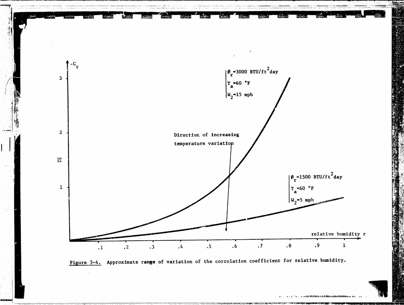
.,~1&· f ...

" ' ..SJ iq '· ! < i

~

~ l ,J

··.,1 ~-,-!

1 I

3

2 .

l.l1 N

1

"'

-C r

~ •3000 BTU/ft2day

r

T •60 °F a

w2•15 mph

Direction of increasing

temperature variatio

0 =1500 BTU/ft2day r

T m6Q °F a

I J -

1

-: relative humidity r

.1 .2 .3 .4 .5 .6 .7 .8 .9 1

Figure 3-4. Approximate ranse of variation of the correlation coefficient for relative humidity.

"' •• t ..... • .• ~o.t:il.i!t.:~UJij~.J£\,jj,l,i.,, •• ,.jlu.liA!A.li»~ ... ; ....

,,-- ~·~ JN4fl ... t.J](II3l)IW.;;:i(t,I.4W"~:·.

. - . ' "' ~ l -\. ..

f/' ~ I ~ f '1 :I 'i;. • • .I

~~--·~!.{ _ _. __ ,~~·- --~---·~

IJ1 w

4

3

2

1

.l.'~ijULC: .,)" "'Y • ••t-t--~._-..

-c0 r

15,000

tb ..

. . ,..; ---r·••--- --·---.;,..,..~ ........ - ••••--·-~ --~·~--.--- -~ .~ ....... -~- ·-··

T z6Q °F a

w2•5 mph

r -=.75

Direction of increasing temperature va~

T =60°F a

w2=15 mph

r = .. 2

f/J (BTU/ft2 .day) r

Net radiated Flux ---~

-~-r--------~-------,r--------r--------,--------,r--------r-------,r--------r--------~------~-----~~~-- ' -~

20,000 25,000 30,000

Figure 3-5. Approxfmate range of variation of the correlation coefficient for the net radiated flu~.

li.," .' \,

I I I

----,--~~·----------~------~~--~--~--~~--~--~~--~------,.-- --.-.---,. •• ~ ~ ' " ..... ---- ~· .... <

-·-".,.__,.. __ ~ • --.v•·-·-•~• -·~~·-~ ---- --""-•· . ~-------"--~-- ~

.4 ~

I ,.3

lJ1 ~

.2

~1

________ ,......_..,..__...,~~--..--- ~--·-

CW2

~~

/

·r •60 °F I a r •.75

f} •2500 t'

T •60 °F a

T =.5

2 BTU/ft day

¢ ~1500 BTU/ft2

day r

_,.,.... c & .... t: -- I 1 ° ::: ••• ' •• i • ·i •

< ' ' ' 10 15 20 5

!!(ure 3-6~ Approximate range of variation of the corrolation · coefficient ·for the wind velocity.

wind velocity w2 in mph

-~- ------···· .1 --. "' #' •.• -··"'lfi'i'· , . ..,....,. ... _"_~· ... - '.. .... • • ·~ - '"'"· AtE ~-:MO!!JI"'"'\\I!'I!\'IIIIIIIfiiii!'.IRII{IIII!IilfJIIIJ11tJIIIi!'ll•lll'lliiJ . . ;·ill"'' ' ••WI.i¥12t 2$UIIC t•P I . lllllf¥/.~hbtQM

~ ~~,:-~'~. t ~ k '- ;!o • • ·, • ' ~ l ~ ,.. \'·.o ~·· .

·-tr.~

~ l·.;,d ,, ., ' • ·l "- • ,.IT . •

_,~A-~ ..__ •"• ---- '~·~·~·~----··

-CT a

40 50

-- -~ -· ~~-~ -· ·--· --~ -~'-----~-~----~.~~----~ -· ...... -----....... ~- ,....._ .. -~.\-:. -.~ ...... ~

2 0 =3000 BTU/ft day r

w2=15 mph

r =.75

!.-----,r-----,..-----.------y------ . 60

2 ~ =1500 BTU/ft day

r w

2=0 mph

r =.25

70

_..

T °F a

Figure 3-7. Approximate range of variation of the corrolation coefficient for ambiant

temperature.

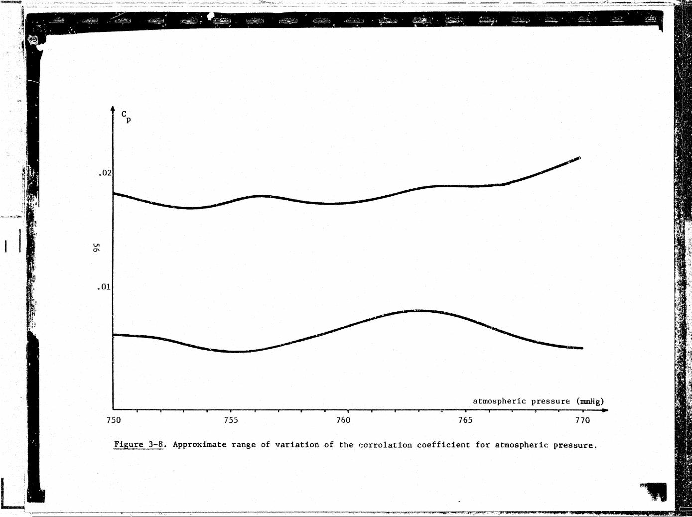
IOillll!""'il!!!l'

I

+ c p

.02

\J1

"'

.01

750 755

~-._:.~-- -J'.

atmo:;pheric pressure (mmHg)

760 765 770

Figure 3-8. Approximate range of variation of the r.orrolation coefficient for atmospheric pressure.

U' - ~ ~ .. _ ... ·~ --···~?""'· .......... __,-, ....... =·--·CCI! ····-" .,--------..,.,_----·--;:--' ~ ·>r.~_,.,, •• ._., ____ <_

i

I!

l i 1-(

I I I

I

i I

I. !

':

i.

I I

I ' '

' I

I,''~,

.o

"

-

IV· UNSTEADY MODEL

For highly variable flow conditions, such as in estuaries and

reservoirs, the hypotheses made for the steady temperature model described

in Chapter 3 are too far from reality to be considered. Taking average

floW conditions would damp out the time variation of the local temperature

and there is even no certainty that the results obtained would be the

average valuE's of the temperature. Moreover, the time variation of the

temperature is an important factor since its amplitude can be large and,

when an average value would be sustainable for aquatic life, it is possible

that the peaks could exceed the lethal limit. The additional stress placed

on living organisms by repeated temperature variation is another reason

for developing an unsteady model.

If the time variations of the flow characteristics are lr:>.ken i.nto

account, it is also necessary to consider the variability of the meteor-

o1ogical conditions. This is one of the major reasons for modifying

the model developed by Dailey ~nd Harleman (1972) which does not allow

for such variations.

4.1 Qescription of Dailey and Harleman's ~odel

This model is divided into two parts: a hydr&ulic part and a

water quality part. The river or estuary network, which can include

tributaries and islands, but no internal control structures or dams, is

divided into "reaches" which arc connected at "node points". Fl\)W j unc-

tions and separations must take place at node points, so that the reaches

only contain lateral injections of wastes or lateral inflows whose

57

-·

I

• i .,

I ~ ...• ~ . : ~

-r. " ,, : ~ '

I -j : I Jl -j f,

~~ • "1

. t

I -,..I

l! "I

~

.-i

......J

T

characteristics are independent of the flow situation in the reach. So,

lateral inflows can account for surface runoff or pumped storage devices

but not for tributaries since the discharge of the tributary at the june-

tion is influenGed by the discharge of the main flow. A typical estuary

network schematization is shown on Figure 4-1 taken from Reference 1.

In the hydraulic part, the equations which govern the flow are

solved in order to obtain some of the flow characteristics which are

required for the water quality part. Those equations are the continuity

equation:

.:2~ + i!Q ~it t.JX = (~-1)

T.vhere

A = . f h . (ft 2) cross sect1cn area o t e r1ver or estuary

Q = discharge of the river or estuary (cfs)

= lateral inflow per unit length of the channel (cfs/ft)

and the momentum equation:

where,

(.)

c

,j (AU) + 2_ (QU) 1t ax

Jz + u:ul~ =-Ag( __._+ dX C2 R

z h

d (. ~)

lX

U = cross section averaged velocity = Q/A (ft/sec)

g = acceleration of gravity

= Chezy coefficient z

(4--·2)

~ = hydraulic radius of the channel

p = fluid density

d = depth to the centroid of the channel cross-section c

58

. . . r 1

~-~Ji":.. ; ... ' ~· I "*· lJ' • .:

--

·-

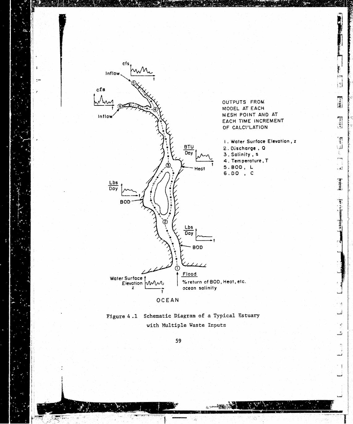
r

cfs

lnf!ow~1 5 ,

cfs ,

f '~ 'i..,

~~;~: Inflow ' -~\

~~

~\ BTU

~~y~ /J " ' t -Hect /.r 1""'\l ~

Lbs // /f' Cloy f "-"-... i { { •

'(_~:._~- t ;.1 : \ ~ aoo~-~ \ ,._ ) : .. ~ , ~u~

/ ,\·,, )( ® ''. . Lbs f

.. \. t-. Day L:::::t \ BOO ~

/~~ <D

OUTPUTS FROM MODEL AT EACH MESH POINT AND AT EACH riME INCREMENT OF CALCt'LATION

I . Water Surface Elevation, z

2. QjscharQe • a 3. Salinity , s 4. Temperature 1 T 5.800, L 6.00 , c

"~~ Water Surface ~

Elevation ~1\J 1. -~

t

t Flood

~·~return of BOD, Heat 1 etc. ocean salinity

OCEAN

F:tgure 4 .1 Schematic Diagram of a Typical Estuary

with Hultiple Waste Inputs

59

• ' .. ~ .. .t.

. .. ... \" • ".· ~ 4. ~ . ... . . •• . 1• • ~ ( ' ,~ \. • ' "" ' ' '"'• r ' \. ,Jfl , t -' \ ., r ' • .. V , '

,., ' !

'; i .

i.:-:,

l lJ

'"lr\ ;~; L~J

~ ;: irb .... <'

t_!j '•i

; r ,_j

·1

* ....:::!

~·1

_.;; !

.. l ........J J

1

d TtE term - Ag _£_ C!p accounts for the density variation along the let'igth

0 ax of the channel. This density variation c3n be caused by the salinity

intrusion but also by a temperature variation. Though, this last

effect is not included because of its small magnitude.

This set of partial differential equations can be solved provided

one initial condition and two boundary ccHditit11.s are prescribed. As the

model now stands, those initial and boundary conditions can be specified

either on the free surface elevation from a fixed horizontal datum or on

the discharge. Although other variables could be used such as the average

velocity or the cross-sectional area, the elevation and discharge are

the more likely to be available from gauge or control structure measure-

ments.

Tn~ finite difference scheme used to solve those equations is

described in detail in Reference 1 and has not been modified here.

The water quality part solves successively the equation governing

the distribution of salinity, temperature, BOD and DO. Our only interest

here ~s in temperature and the corresponding equation in the model is

J;)t (AT) + ':lat (QT) = ..]_ (AE aT) K A (T T ) + S

Q ~x 1 Jx - T - E (4-3)

where S is a source term accounting for waste heat discharges or lateral

inflows heat input.

The assumption made of a constant equilibrium temperature TE both

in space and in time allows to write

d =- (4-4) ax

60

":'

J 3 ~ n

" ':! .. ~ ... -..

_, ~ .... " .., : . ~

l : 1

'' 1e

t i l 1i

In age

:st

' al

>th

since, = Oll Equntion 4-4 is Lhen cquiv.Jlent to

.L A + _a_ Q = 0 ( 4-5) j)t (}X

• which is tha continuity Equation (4-1) with qL = 0. This shows that,

actually, Dailey and Harleman's model is only valid, for temperature,

when q1

yiC'lds

where

= o. In that case, subtracting Equation 4-4 from Equation 4-3

(4-6)

/\TE = T - TE

In order to later show how the modifications were introduced in

the model to account for the variability of the meteorological conditions

and for the proportionality of the surfa~~ heat flux to the surface area,

a summary of the numerical scheme used by Dailey and Harleman to solve

Equation 4-6 is now presented. Parts of it are directly taken from the

original work (reference 1).

For easier notation let us set tTE = c, and Equation 4-6 becomes

a at (Ac) + a ;) I

:)x (Qc) - IJx (AEL ,~ ) + "K.r Ac - S = 0 (4-7)

Each reach is divided into elements which lengths are not necessarily

constant and a linear variation of all the terms .z.n Equation 4-7 is

assumed over the elements. (r~. being the value of the variable nat J

mesh point j, the linear variation is realized by introducing interpolating

61

l 1

functions ~. defined as shown on Figure 4-2, and the linear interpolation J

for the variable a is realized by the equation

M li = }:

j=l 4>. (a).

J J (4-8)

1 2 3 j-1 j j+l M

Figure 4-2. Definition of the interpolating function ¢j.

Performing this interpolation for all the variables in Equation 4-7

and substituting them in Equation 4-7 yields

+ K •T

M r.

j=l

M + .,() [ r.

nX • l J=

~ (Ac) . j J

4>. (Qc) ·] - -:-);) ( ~ J J , X j=l

M r.

j=l «t>. (S).

J J = R(x, t)

;p. (AE ~ ) ] J L ax .

J

(4-9)

a residual R(x,t) exists because this piecewise linear approximation does

not match exactly the solution.

The method 1f the weighted residuals is then applied in the form

of the Galerkin's method, where the residual is weighted with the

62

~l

I !

r

l t j

l

l I !

1 l

t ::ion

j. i i ,_

. ; ;

,! '1 I

i

j l t

I ! ' l;

r l ! :

I I, t; l; 1 I' ' i '•

1 f: 1 i

n 4-7

does

rrm

interpolating functions,integrated over the length of the channel and

set to zero. This integral ca~ be expressed as a sum of integrals over

the eiements:

Jwi R(x,t) dx = ~.:J~. R(x, t) dx = 0 E ~

for i=l, 2, • • • , M (4-10)

which r::.>w gives M equations with M unknown values of c at each time step.

Those equations are

M

f J >.: ¢. ~ ( l: E ~ u j =1

<i>. (Ac).) dx J J

+ M }: r <i> • + ( [ <jJ • ( Q c) . ) dx

E j' ~ c.X j=l J J

)~ Jcp. '?13

M M ( ac . ) ~I $iKr

)~ ¢.(Ac). dx - ,~ ¢. (AE1 -) dx + .

E ~ tX j=l J ax J j=l J J

f<i>i M

- >: >: ·:·. ( s) . dx ,. 0 E j=l J J

i = 1' . • ' M (4-11)

A number of approximations are t~en introduced to transfo~n Equation 4-11

to a more solvable form.

(1) The time derivativ~ of the storage term is approximated as

a simple difference:

d M a (Ac) '::" 1.: ¢. (A.c.)

;)t j=l J at J J

A~+l -n+l A:l -n M c . c. ~ r. ¢. J ] ] L (4-12) j=J. J Llt

63

'· '· '

·--

' '

. '

where

-n c. = discrece value of c at mesh point j at time n J

This difference approximates the time derivative best at time

~t 1 t + 2 or (n + 2 ) l\t.

(2) £he remaining terms in the equation are approxtmated also

. + At at t1.me t 2 by averaging between times t and t + At.

For exFmple, the advective term is:

() 1 (Qc) ~ -ax 2

a M n+ 1 -n+ 1 M n -n ;) ( }. '-ll • Q . c . + }: •il • Q . c . ) lX j=l J J J j=l J J J

(4-13)

(3) In the dispersion term, the coefficient AE is averaged

over each element and c is assumed to vary linearly:

M -n+l i. •1>. c.

j=l J J

where AE = average of AE over an element

= ~ {(AE)~ + (AE)~. 1 } for element j, j+l ... J JY'

M -n

>: 1>.c. ) j=l J J

( 4-14)

Assw~tion (3) is necessary in order to avoid having the disper-

sive flux integral in Equation (4-11) ~sult in gradients of c rather

than value of c themselvec at the mesh points. A consequence of this

assumption about the f-\ispersive flux is a discontinuity at the mesh

points. This discontinuity can be shown by integrating the dispersive

flux integral by parLs:

.;;r:~·---7'':":~'"'~~ :t •

64

r>, L

r I

I l i I ;

i'

I l

l

' I I

i'

X

>: 41i () (AE ()c ) dx • r <P. AE ;)c J i E ax ax 1 ax xi-l

X + [<ll, AE :)c] i+l

~ ()x X. 1.

>: d<!l, --~ dx

AE ac dx ax i = 1, ••• , M (! .. -15)

E

Noting that

1. = 0 at x = x. 1 ~ 1.-

4>. = 1 at x = x. 1. 1.

~i = 0 at x = xi+l

the terms in brackets are

AE ;Jc ;)x

x=x. 1

element i-l,i

x=x. 1.

(4-16a)

(4-16b)

(4-16c)

(4-17)

element i, i+l

= (dispersive flux into element i-l,i)+(dispersive flux into element,i,i+l)

In the physical system this sum is zero; however, it is non-zero in the

numeric.11 .:;.~heme because of the piP.cewise linear approximation. Never-

theless, the physics of the sys tt~m are assumed to prevail, and the sum

of the two terms is set to zero, <"xcept at the boundaries. There, only

one of the terms appears, which corresponds to a natural boundary condi-

tion in numerical methods which are based on the calculus of variations. I ' .

f 65

IJ '

. . • l. , • . .

, . .... .. ~

To simplify che notation, the dispersive fluxes at the boundaries

will be written as:

-AE ac ()x

AE ac :lx

•

x=x M

1 = dispersive at time (n +

2) 6t flux into upstream

boundary

(4-18a)

1

= dispersive fh~x at time (n + ~) ~t into downstream L.

= - 'M ()iM

boundary (4-18b)

whert: oil and oiM are K~unt::cker deltas tn matrix notation.

Introducing the results of Equations (4-12) thf'~Uih (4-18) into

Equations (4-11) yields:

.. M f M ~ n+l -n+l f n+l-·n+l dx + .6.t dx I. •ll.( r. <j).A. c. ) E<P.(1: d Q. c. ) E ~ j=l J J J 2 F. 1. ·=1 X J J ... J

t\t ): AEn+l f d~I M dct>. +l + K6t r F· < ~ <t>.A~+l~~+l) +

__J_ -n dx dx 2

( ~: d c. ) E L dx j=l X J 2 E l j=l J J J

= f M n -n

~ <P.( [ ¢.AJ c.) dx E 1 j=l J J

Llt --2 f

M d<P. ~ n -n

E ct>.( E d Q. c.) dx E 1. j=l X ] J

L\t -:--=n l , -n K.6.t . .;. ... - fd<t>.. M dtt>. E AE -:. ( E --'- c . ) dx ---

2

[ M n l: J4>. ( r. ¢.A. E 1 j=l J J

~~) dx J 2 E L dx j=l dx J

1 n+-¢. S

2 dx, i =

1. + n

1At 6 .

1 - ~llt o .M + llt E

1. .£ 1. E 1, . . • M

(4-19}

Appendix A con~ains a summary of the values of the integrals in Equations

(4-19)~ With these values, Equations (4-19) may be written in matrix

notation as:

66

- • • Q .. • • .. ... • ....

• I ' <,. \ \ . .. . . \ . . ..

fi ~

'

l;

~ies

1m 1dary

4 • ~am

.t: 1dary

'\

l \ ' 1

i ' !

f ' i i l

t;'

to

lations

.X

-n+l A c . - =

-n D c + e = (4-20)

The coefficient matrices ~ and ~ are defi.n~~d in such a -way as to emphasize

their tri-diagonal nature. To save ~otation and execution time in the

computer, the individual mat~ix elements are evaluated in terms of certain

factors which can be calculated once and used repetitively thereafter.

A = =

where

ai =

i a =

H a =

i c =

bi ·-

;:, ~ '. }~ '. (-· , ...

1 a

1 c

2 a

2 c 0

0 M-1 b

M-1 a

2£2 n+1 fl,n+l fl,n+l

~1,2 A .. + 1 4 1

2f2(/.\i-1,i + n+l fi-l,n+l

/'::. . . +l)A. + 1,1 1 1

2£2 An+1 fM,n+l fM-l,n+l

~M-l,M + + M 4 1

£2 An+1 fi+1,n+1 fi,n+1

/1. .+1 + 1,1 i+1 4 1 '

£2 l'::.i-l,i An+l fi-l,n+l fi-1,n+1 i-1 4 1

67

·:: ... '\, 4-t. ,t_,~ .. ~-

+

1

'

M-1 c

M a

fi,n+l 1 ,

< i <

2 < i

2 < i < M-1 -

M-1

< M -

1\

li i n ; !

t. j

i " i

"""'1 J ' ' ~- I

_, ~ ' Lj

~ i

,, j

9 l .I

t J

rr;q ,, ' ~

li t:"'~~,

f f!' --~:I I

··--~~

~._.;ti

f ";'1 h\

"1 \..

and

D = ..

where

An+l En+l ; An+l En+l fi,n+l i i '{" i+l i+l

= 1 Ai~i+l

f2 1 (1 + _K~t) ::;; ,__

6 2

f = l ( 1 -· KL\ t) 3 6 2

Q~+lt.T fi,n+1 l. 4 ~ --~~--

rd1 dl a c

2 d2 ?

db d.'-a c

0 ~ ,, 0

M-1 db

L

dl zr ll1,2 An +

_l.n = t ..

a ~ 1 4 :J

di = 2f3 (/\. 1 + l\i, i+l) A~ a ].- , i l.

dM = 2f3 /j ~ £M,n fM-1,n a M···l ,M - 4 1

llt

4

fi-l,n 1

di f3 n fi+l,n fi,n 1 = l\. '+1 Ai+1 + ' 4 1 c l.,l.

68

fi,n 2 < i < M-1 1 J - -

< i < M-1 - -

. ' ... ,. ... "' . ~ .. . . . . I . a • • , • ' '

. .

·' .. j 1 l

j J.

I l

! '

j !

',~

! '

di = f n + fi-1, n + fi -1, n 2 < i < M b 3 t\-l,i Ai-l 4 1 '

The vectors c and e are defined as:

-n c = e •

Initial and Boundary Conditions

r1. L'lt + (source terms) 1

(sourc~ term)2

(source terms) 1 M-

- rML\T + (source terms)M

1

The set of M linear equations represented by Equation 4-20 is

1 d h · · h f · 1 ( -n+ 1) · so ve at eac t1me step to b~ve t e temperature pro 1 e ~ g1ven

-·n the one At before (~ ). It is then necessary, in order to start the

-1 computation to specify the initial temperature profile {~ ).

Though, Equation 4-20 contains M+2 unknowns: the val~es of c at

each of the M meshpoints and the two extreme dispPrsive fluxes, n1

At and

n2

~t; and ~ of them are to be specified as boundary conditions, at all

times, to allow the resolution of the system. The easiest choice would

seem to be the 2 dispersive fluxes, but their determination requires the

knowledge of the extreme temperature gradients, which are, in the general

case, more difficult to obtain than the temperatures themselves. So the

program is set to handle both types of boundary conditions.

4.2 Modification of Dailev and Harleman's Model

The exact equation for one-dimensional, unsteady heat transfer

69

-

l ,.,

l L j ' t

j LJ

.,

' i I' ~

,f ·.

~" 1

}'

c

r •

li . I

I'

__ ]

j' ! '

I.

i

i I

is Equation 2-1 and assuming the product pc to be constant over the range

of temperatures considered yields

a a a aT b0 WHD + THD (AT) + -. (QT) = - (AE - ) + ___n + (4-21)

()t ax ;)X L ax nc pc

and it is easy to check that

used in Equation 4-3.

WHD + THD pC

is equal to the source term S

If we consider the meteorological con:.itions as variable ~ith time,

Equation 4-4 is no longer valid an<;! the linearization of the surface heat

flux does not bring any simplification since ~TE cannot be isolated.

Moreover, if the model is to be run for long periods of time during which

the water temperature varies greatly, the dependence of the water tempera-

ture on K has to be taken into account. So, it was chose, here to direct-

ly detnrmine the net surface heat flux 0 through Equation 2-24 at each n

meshpoint and time step.

Equation 4-21 is similar to the one solved in Dailey and Harleman's

model (Equation 4-7) from which it differs only by the flux term. It

was not thought necessary to write a new pro~ram.

In order to keep as much as possible the structure of the original

program, the decay term was simply eliminated by setting the decay coeffi-

cient to zero in the data set; and the new value of the surface heat flux

was introduced as a supplementat•y term.

Keep~,ng consistent with the original numerical scheme, a piecewise

linear interpolation of b and 0n is performed between the mesh points.

b0n 1

- ·-PC PC

70

,, " H

' .

I I

t l !

l ! I

i

J , ' (

! -~ I ! 1

r

s

and Equation 4-11 becomes

1: Jrt> _1_ E i at F

a M ( L 4>.(Ac).) dx + L ¢.--a ( L $.(Qc).) dx j==l J J E l. X j=l J J

L fc~. E J' l.

M )~

j=l q>. ( S) . dx = 0

J J

where c now stanaG for T.

1 pc .. r .... _._rrt>i_ ~ !l>-l (b0 ). dx ~.J~ j-""1 J n J

i = 1, ••• , M (4-22)

According to hypothesis (2) previously stated, the new term should

. d . + t\t be approx1mate at t1.me t :z It should be noted that there is no

. 1 ~ k' + ~t rat1.ona ror ta 1ng t :z rather than any other valu~ in the segment

[t , t+At] except sim~licity, but this approximation was conserved here

because an iteration would require a complete change of the structure of

the program.

This approximation is

;; Jet'. E l.

M 1 f M _, _[

1 [ tj (b0 ) . ] dx = -

2 I ~. 1: r <ll. (b0 ) ~ 1 dx

J- n J E 1 j=l J n J

·f M n+1 t 4>. i: [ •L (b0 ) . ] dx E 1 j=l J n J

(4-23)

Thougt~ 0 is unknown at ~ime (n+l) ~t since it depends on the water n

temperature at that time, which is what is being calculated, and the func-

tional relationship between 0 and the temperature is too complicated to n

allow an implicit resolution. So, the temperature is taken at time n ~t

' j

.J

..

.J

only, which gives ~

71

. . . ,.. .. . 10 • ' I

(0 ) n+l/2 n j

which is furthermore approximated to

MC~ + MC~+l ( _,.,_] __ ...,..]_

2

so that Equation 4-23 can be approximated by

}.: fl~. E ~

A-. _1 J [

b~ + b~+l '+'j 2

and the new form of Equation 4-19 is

r M n+l ·-n+l ilt f M d<t>. n+l -n+l >: .~,i ( >: q,. A. c. ) dx + -2 f. <P. ( >. -d....l Q. c. ) dx E ' j=l J J J E ~ j=l x J J

M

(4-24)

(4-25)

(4-26)

+ 2.'\t E AE n+l -~ ( }.: --l c~+l) dx = 1• d<P. M d•P.

2 E L dx j = 1 dx J fl n -n L <P.( f. <t>.A. c.) dx E ~ j=l J J J

llt -- 2 J :H d •11 • r d <P • M d <f> •

>~ 4>. { >: _J_d Q~ ~~) dx - ll2t Er. AELn dx~ ( f. ---ld c~) dx E ~ j=l X J J j=l X J

E fcfl. ~ tfl. [b~ + b~+l 0 ( MCj + Mcj+l E ~ j=l J 2 n 2

-n ] cj ) dx

(4-27)

which can be written in matrix notation

-n+l A c =-

- D en + e + fn+l/2 =- (4-28)

72

'

I l J

I J

where~, £n+l, e• ~nand! are the same as in Equation 4-20, with K = 0,

and !n+l/2 accounts for the new shape of the surface heat flux term.

Tak!.ng the correct values for the integrals, as given in Appendix A, the

elements of the new matrix f are

£~1/2 r ~1! 2_ (0nQ)~+l/2 t:\1 2 (0 b) n+l/21 At = + -=...z..=,

-1 L 3 6 '~n '2 J pc

fn+l/2 [ ~i-1, i_ (~ b) n+l/2 ('~i-1,~ + f:... "+12 (0 b)~+l/2 = + ~;~

1 6 n i-1 3 n l.

+ 6

i,i+l_ (il b)n+l/2] t:\t 6 n i+l pc

fn+l/2 = [ 6M~l,M (0 b)n+l/2 + llM-l!M (ll b)n+l/2 J ilt (4-29)

M n M-1 3 n M pc

The initial and boundary condition requirements are the same as

in the original version of the model.

4.3 Test Run

In order to test the modification introduced, a run was made for

a steady situation with the same conditions as in t~~ sample run of the

steady model described in Chapter 3. The flow chara{'terisLtcs needed for

the steady model were the discharge (taken as 1000 cfs) and the width

(taken as 1000 ft). For the unsteady model, since the hydraulics are

computed through the continuity and momentum equations, more geometrical

data is required. The depth was chosen as 5 ft. which gives a cross-

section averaged velocity of 0.2 ft/sec. The required Manning's coeffi-

cient was chosen as 0.02 and the slope was computed through the Manning 1 s

73

t

r f

I t

~ t i ~·

t

~I . I

rl _ .... r

·r ,r .,. • .. • • : • ."" _..,. ' .... - - ~ + - - - • '1

. . '

t ¥

equation to be 0.854 10-6 ~o ensure a constant depth with distance.

The meteorological conditions are thE! same as for the s::.:nple run

of the steady model~ namely

T = 60°F a

r = .75

0 = 2500 .dTU/ft2 day r

p = 760 mm Hg

and the corresponding equilibrium temperature is 52.8°F. The dispersive

coefflc:ient is internally computed through the Taylor equation

= 77 n U ~516 (4-'30)

where n is the Manning's coefficient.

The upstream boundary condition was specified on the temperature

itself (61.4°F) and the downstream boundary was specified on the disper-

sive flux which is imposed to be zero. This implies a zero slope of the

temperature profile at the downstream boundary which is not totally exact

sine~ the temperature decay continues to infinity, but this condition

allows a better verification th:An imposing the temperature at the down-

stream end from the results of the steady model. The length of the per-

tion under study was chvsf!n to be long enough to allow an almost zero

slope o.f the temperature profile, and thus approximate better the down-

stream boundary condition.

The initial condition was chosen as 58°F all over the 50,000 ft.

of the river portion under study.

This run describes the evolution of the temperature profile

74

in a river initially at uniform temperature (58°F) larger than the equil-

ibrium (52.8°F) in which, from time t = 0 onwards, the upstream incoming

.I

j i ~acer is at il.4aF. The temperature p~ofiles after I, 2 and 3 days given

I I'

by the unsteady model are plotted on Figure 4-3 which shows the simultan-j

J. t +

j

eous progression of the hot water front and the general temperature decay.

The mean velocity being 0.2 ft/sec., at time 265200 s (3 days),

the hot water front traveled approximately 53,040 ft. and a steady state

l

I days matches almost perfectly the one given by the steady model.

should be reached. This is verified as the temperature profile after 3

i

! !

75

60

....., 0\

55

50

J I

-·---~-·~·~-,---. .......... ,.~.....___ ...... .__c_~ _, .. _......._ _____ _. -~-~~..._....., """" ~-''"' -. . ..-..• ~- - -- ~-~..-._~ ~·,·• •• __ .....-.....__ ·- •~•'-• --~-•- ~---·• ••---·--• .. ....-............... .---~..-.,_._,,_,~,.----.~---'"'""'""---•-.-.------·---· -~•

Temperature {°F)

time t = 1 da

)(

Temperature ~rofile as given by the steady model~

Results from tne unsteady model

in:f.tial temperature

time t = 3

tiw~ t =_2 days

Equi1~brium temptra~ure ____________________________________ , _____ .._.--

distance (ft) .-------.-- • a 1 • a a ' w-1 • t 1 • 1 1 • 1 • ; 1 ' ; w a 1 =- _.

10,000 20,000 30,000 40,000 50,000

Figure 4-3. Test run with steady river parameters and meteorological conditions.

~---~--- ---~

______J'~-------------------------------------------------------------------------------------------------~---

V. CASE_2_T_UDY: CONOWINGO RESERVOIR

5.1 Natural -~-~mperatur.e D~~tributio~

1 The ability of the modif~ed versjon of Dailey and Harleman's model

to predict temperatures as a function of distance and time under varying

meteorological conditions was tested on the Conowingo Reservbir, located

on the Susquehanna River at the border between Pennsylvania and Maryland.

This reservoir, a map of which is shown in Figure 5-l, is situated between

Holtwood Dam at the upstream end und Conowingo Dam at the downstream end.

The reservoir is also the site ot: the Pe.1ch Bottom Atomic Power Station

and of the Muddy Run Pumped Storage Generating Plant. The flow in the

reservoir is governed by the ope~ation of the hydroelectric dams and

pumped storage plant, so that it is highly unsteady and reversals of

the flow direction occur at fretfuent interva l.s.

The modified mathematical model was applied to determine the nattlral

temperature distribution in the reservoir as a function of time. Natural

temperature refers to the temperature in the absence of heat addition

by condenser water discharge from the Peach Bottom Atomic Power Station.

Because of the one-dimensional nature of the mathemati~al model in

which T = f(x,t), the calculated temperature at any given time and distance

corresponds to the temperature averaged over the (:ross-section of the reser- '

I voir. Observations of natural temperatures in Conowingo Reservoir show

that, except for a s~10rt period in late summer, there is relatively little

I temperature stratification. This is especit!lly true in the upper portion

of the reservoir where the average depth ls less than 20 feet. Thus the

utilization of the transient, longitudinal temperature distribution model '

seems to be justified. 77 I '

I

... ~t:~··*~

Jf'i

,. J

-~--~--"~--~---- _, _ ___,. ·~-· ---"-'-'-·~- ),..-..._._,_,,__ ~..J -~ ...... ~~--·- .,_...,.....~• ----~- ,__-, .. ,.--o......;---'"< •-··--,;,...--"-·-•"-'•••-., ~ ---~ . ..--.. ........ \.,--o------•,.,...._.•, J·----~

........ co

Holtwoool Dam

P•oc:h BoUotn Atomic Power .5tQtion

I .

/~ ,<(

1: .t

Conowinso Dam

.,..,.-------~'---+-----__

]I !I ~· X

~I ~·

I

I

.. N

.... 0 1•''• ,,,,,&t•••f nu t

Figure 5-l. Map of the Cbnowingo reservoir showimg the schematization used for the model.

U• ~ -~ ......... it4'fl --~···'·'"··~~-....... .....,""""'l"o!

·:::.~.

The pred-l.c.tive qualities of the model are required by the ultimate

aim of the study which is to determine the temperature excess over the

natural due to the operation of the atomic power plant. For that purpose

the model wi.ll compute the na":ural temperature, given the meteorologil·al

conditions and bo\Indary conditions independent of the heated water dis-

cl1arge. The temperature excess will be determined by subtracting the

calculated natt1ral temperatures from the measured temperatures in the

reservoir during operation of the power plant.

1'he portion of the reservoir in which the temperature distribution

is of primary interest is between the upstream end and the state line.

Therefore, the reservoir was divided into two reaches with a junction node

on the state line, as shown on Figure 5-l. It was necessary to extend the

model to Conowingo Dam in order to have adequate downstream boundary condi-

tions. The upstream boundary (node 1) was shifted south from Holtwood Dam,

to the point where th~ lake proper hegins, to avoid a section of very

shallow water which contains cascades and supercritical flows and for

whicl: the hydraulic part of the model cannot be applied because of limited

topographical information.

For the hydraulic part, the mesh spacing was chosen as 1500 ft. and

the time step as 720 sec. The discharge versus time was specified as the

upstr~am boundary condition (node 1) equal to the sum of the discharges from

Holtwood Dam and Muddy Run Pumped Storage .Plant. In this sum the discharge

from Huddy Run was taken as positive or negative according to whether the

Will..er is flowin~ into or pumped from the reservoir. The downstream boundary

(node 3) was specified on the elevation ns a function of time at Conowingo

t>am. All the data for the hydraulic part was taken from the operating

sclwdules of the dams and pumped storage plant. 79

-~

I i ,. j

I I

j ·~

' ;; ~ ~

~

l R

L.J

c:t;'

'-1

l

~{

J ' l ' l

r !

!

~' l.

-j l ' .... ..~

~~

I ~,-

_;I ' .,..,. · • ' . . I ~ I, 1 ' • • ;-- ~- • ' • • • f. 1 ,

.!_:~--' ... •• . ~ . .'1\ , '""" \ l ., • ~ ~ ' • .·~ - g • • • t.. . . , . 0 • • ''. • ·• . ·~ . • .. /

-'

'1

For the temp~rature computations the mesh spacing was chosen as

500 ft. and the time step as 720 sec. The upstream boundary condition

was specified as the tetnperatura versus tine, whten the dire!ction of. d'te

flow was downstream at node 1 and as the dispersive heat flux, AEL ?T , dX

when the flow direction was reversed. In the latter case the dispersive

flt~ is computed at each time step as well as an esimtate of lts variation

rate, thus allowing an approximation of its value at the next time step

which is used as boun.dary condition. This type of boundary condition,

which is similar to the one used at the ocean entrance in the case of an

estuary, was tnken to ensure future independence of the boundary condition

from the heated water discharge of the power plant. Otherwise, when the

flow reverses, the influence of the heat source due to the power plant may

reacl1 the upstream boundary and the subsequently computed temperature dis-

tri~ution would not be the natural one. The original model provides for

such a boundary condition, but the incoming temperature is specified as

constant with time anc a change had to be made to allow for the temporal

variation. The downstream boundary condition was specified on the disper-

sive flux of heat which is imposed as zero because of the presence of the

darn which breaks continuity and only allows advection. The longitudinal

dispersion coefficient EL was chosen as 100 times the Taylor value as

given by Equation 4-30, to obtain the best compromise between exactitude

of the results and stability of the numerical scheme for the longitudinal

t~mperature profi 1 Ps 4 Such a ratio is tvelJ in accordance with measurements

made on the Miss bwippi River and reported by Yot:sukura (196 7) which show

that for high values of the width to depth ratio (about 300 in our case)

the longitudinal dispersion coefficient can be as high as 200 times the

Taylor v?lue. Large values of the longitudinal dispersion coefficient ro

f

I

also tend to. smooth the numerical instabilities in the temperature profiles·

as can be seen by comparing Figures 5-7 and 5-8 which show the computed

profiles on September 2, 1972 at 24 hours with dispersion coefficients equal

to 100 and 10 times t:he Taylor value.

Two runs of the model were made; one for a period of 3 days starting

August 31, 1972 at 24 hours (Julian day 235) and ending September 3, 1972

at 24 hours (Julian day 238); and the other one for a period of 18 days

starting Apri] 7, 1972 at 24 hours (.Julian day 93) and ending April 25 at

24 hours (Julian day 116). These periods were chosen due to the availability

of me~a:surements to provide boundary conditions and to check the results of

botlt the hydraulic and temperature predictions of the model.

Plots of the outputs of the model for reach 1 are given on F!gures S-2

ttJ 5-8 for the September run and 5-9 to 5-13 for the Apri. · run. The results

for reach 2 are generally not given dS insufficient measurements were avail-

able to allow a verification. For both runs, extremely good correlation

is obtained for the hydraulic part as can be seen from Figures 5-2, 5-9

and 5-10. Unfortunately, the only measurements available were that of the

centerline surface velocity which is not strictly equal to the cross-section

averaged value computed by the one-dimensional model.

The results of the thermal part of the model are also in good agreement

with the measurements. Though, for the September run the computed values

become lower than the measured ones as time increas~s. This can be explained

by the fact that the measurements were made very near the surface whereas

the model determines cross-section averaged temperatures. More thorough

measurements made during that same period of time show that, in effect, the

temperature decreases with depth. In reach 1, where the depth varies between

12 and 19 feet, the temperature difference between the surfacE and the bottom 81.

c ' 0 -!4.

I .,

I 1 I

I ! I ,;

t

can be as hj.gh as 2°F. Unfortunately the time of the measurements at

varying depths was not recorded with sufficient precision to allm·l a

verification of the average temperatttres; but the computed values are

well within the probable range, since the difference between the computed

cross-section averaged temperature and the measured surface temperature

rarely exceeds l°F. The fact that this difference increases with time

at the beginning of the run is due to the specification of tha initial

condi tic..m wnich was made on the surface temperature. For the Apr-il run,

where t:he correlation is better, measurements at various depths show

that the vertical temperature gradients are much ]ower.

Another cause for differGnces between observed and calculated

temperatures is the fact that temperature measuremen~H at the upstream

boundary were not available and, when this boundary condition is 3pecified

on temperature (flow in the downstream direction), the data from the

nearest monitoring station, situated snmc 8000 ft. dounstream, was used.

Figure 5-3, which shows the variation with time of the temperature

at the upstream boundary for the September run, proves the validity of

the boundary condition used when the direction of flow reverses. Except

during the first flow rever~al, which is also the beginning of the run,

the computed temperature matches the measured one very well. The dis-

crepancy during the' first reversal comes from the fact that the dispersive

flux, which is used as a boundary condition, is computed from the initial

condition which is s~mewhat imprecise because of the limited number of

monitoring stations.

A~ in many mathematical model verifications, the available data,

although very extensive, proved to be partially inadequate in providing all

82

the information required to run the model and to precisely check 5.ts

results. This 1~ due to the fact that the characteristics which can be

determined with simplicity by measur~ment and by mathematical models

are rarely the same and jUdgement h~s to be 4sed in their inLerpretatlon.

I~ this case study ~f the Conowingo Reservoir, distortions are introduced

in the results because of the lack of temperature measurements at the

location which was dictated as the upstream boundary by modeling considera-

tions, n'd verification is influenced by the fact that only surface tempera-

ture measurements were generally available.

Despite these limitations, it is felt that good agreem0nt exists

between the resnlts of the model and the image of the physical reality

which can be derived from the avai laole, m~~u~m;,ements.

The condenser water discharge structure for Unit No. 2 of the Peach

Bottom Atom~c,: Power- Station is a surface ch<mn~l entering th(:"' reservoir

almost parallel to the shoreline. It is expected that the heated watt•r

plume wiJ 1 r~main attached tl1 the side thus creating significant transverse

temperature gradients. Although the mathematical model described herein

cnn include:! arti.fici~l heat injections, the one-dimens·ional nature of

the modt' I , which assum~s complete mixing of the hen ted e [ f 1 Ut'nt at' ross

the St1etion of the reservoir adjacPnt to th£' putfa11, is not realistic

in Lh L~ si, tu~t t ion. Bec.J us(! of the i ntcres L tn the near field exc.:es1:1 temp-

!:!rat'u.re distribution, tlw nrlJt•cdure outl i11eJ in section 5-1 was chosen.

Sim:e the latet'al gradients of the natural temperature are generally very

small, the excegs temperature t'im hi' t•omrmced by subtraction of the

computed natural temperature front tim me.Jsured temperature once the power

83

. . . . . • . • ;_. -~~ • - .• ' 4• ..... , • : ." . . ,, - •. · •.. J '. • • ••· • I .. :.t \.. .. ' • ., • • . t . ..,

ll -

l

j l , [

.

f '~ !

! ' l

r

~ I ~ r

~ I . l

~ I I

~ I

~ I ~,,

I

~ I I l

plant is operating. This procedure should be fairly accurate even in

the near field region of the outfall structure.

The complete mixing hypothesis inherent in the one-di·mensional

model theoretically gives the least local temperature increases and as

such is an interesting limiting case. Additional runs of the model

j were carried out taking into account the waste heat input from Unit 2

<>f the Peach Bottom Atomlc Power Station (discharge 1650 cfs, excess

I

I temperature 20.8°F). Figures 5-14 and 5-15 show the resulting excess

temperature profiles at different times of the day in April and '

September. The mean daily flow throngh the reservoir during April

is about five times larger than in September. This explains the fact

Lhat peak excess temperaturesat the power plant output lot:ation are

hight>r in September than in April. The larger excess temperatures in

the reservoir upstream of the plant in September are explained by the

fact that flow reversals are common during this period, whereas, during

April the flow is essentially unidirectional. The differences in

the profiles at different times of the day, especially in April, show

the importAnce of a transient model wher~ both flow characteristics

and meteorological conditions vary with time.

84

I

t

(X) Ul

L.

'Ci -v

0 10

can ~N

>-. I

..... -0 0 ....1 w >

~~ .

-en -0 CIO ~N -. >-.....

I -0 0 -l w >

, J . Ill .~. ' . .._ ' ---,. Ill :! r~

Ot::. ____ ........... !""... '" ···-···········'"· -~·-·· ~ ........ ;/'· ·.:·...:: ..

_N ___ , _________ ,,_~ ;~-- -· ____ ...._...._~-~-~ .......... ~- ... ,(.--~---......__~ ...... _._ ,,,--... _ ___._~,-------~J4--.. .... .:.·---··

At X = 13,000 ft

•

237·5

JULIAN DAY •

• Computed average velocity

--- Measured centerline surface velocity

35,000 ft

I ' \ fV \ •

• JULIAN DAY

Figure 5-2: Time variations of the velocity from September 1st t1 3rd, 1972 at two locations

in Conowingo Reservoir.

L. l L = • -~4\!l®:mt.£4 -· .. --- .~:. . .-. ~- .-.. .. ~ ... ., : . . '\1 . ~ 'L .. JWI!!I,!I!t ...... ..!.~~~-·. 1"""-.----~ .. ., __ J.-... -.",.-Jif

r .... --1-'

I'd

Q)

_.-. ~.,, ·-• ----'··~·. • __ ,,_. _._. • •~o-,..,--.-,..

'"~.........,__-~ ~ .,._ --·~· --· ·----~·-~"""--'-" ___ ,.,.,. __ .,__.._~,.-.__~ ... ~~~--~----____.-·-.--------~ __ , • ..,.,._, ___ ......._., _______ ~_ ......... ___ ,-. _____ .. # ___ ._.._._... • -~,...-..~---.;..... ..... .-....:":· \• -· 6~

In periods of flow reversal the boun­

dary condition is specified on the

dispersive flux and the dots •

indicate the measured values of the -o l.L

• Ct QJ "0 -w £r :::> ....

C:> <{ 0'\0:

LrJ a. ~ IJJ t-

co

m 1'--

CX) J'-

r­~

tD

• tl 1

I I I I I I I I I

•

I I I I I I I I I I

' I

' I I I I I

temperature.

Otherwise the boundary condition is ta­

ken as the measured temperature itself.

...._ f'<<<<• ')///,/<<££('1 C(?/?.//4 ,. ·- I ) I I

235 236

Figure 5-J: Time variation~ of tltl' Lt:•mpl'l'dtun.• from September 1st to 3rd, 1972 at the upstream end

of Conowingo Reservoir.

.." ·-.. ·- ~ " ... !Ul,ijQR

-----------~~-~,<-----~------------~·------------ -------~~'\ ~ ..... .,.......,...._...._ <• .........,..,; ti:tolf. ll!C£ ,tt~ ... ~.l

\\

• • ~ • .;.... I ,. ""' • " e:-- " ~ • ... -~- l· - ~

---.~'··- ...

-u.. -(.)' ., -a _...

w tt: :)

~ ..... <( cc ILt 0.. ~ w t-

05 I

V'\ 0 m

m ,....

I

CD r-.

,._ ,....

w t- --. -----

235

u1. l.onuw J. ut;,u 1\.l:!hurvoir.

I

236

Of:. ·"-~~4·

,, ~-~---~~-.,....~---·----~~-~~-~ ~ .. -~ ~--'"'-~--... ~-~---~""~ - --~-·---·· -~~·~~-· ~-...:..~~;::;,

--------------aM--~--._~ ... --~--~0..-............ .m ............ ..

• Measured valu~ of the surface temperature

Computed cross-section averaged temperature.

~ • "- •

TIME (Juljon Day) I .. lh~

237 238

Figure 5-4: Time var i.1Lions of the temperature from September 1st to 3rd~ 1972 at x = 19,000 ft. in

Conowingo R<.•servoir.

\o.....~ ,,..~ ).,..,. oi.-. •f ' • ••••• v .• -~-- # ~··· 1 r . L k¥5 JftS.....,...z I ~

--·~·~~-·,_ __ ___, ____ ,_.,_.,~----···-···'"·~~----~-.-.-··--";c.--·~·------,--- ~ ~=-?;.:-\---... ~-,.-~ .'H">~- •· " ...... ,_-;?:~~~

·-~-·~.r ~)

l .. ~

N CD

-&LCD Dl • 'a -

IIJ a::

m~o (::)~CD

a:: 1&1 0.. 2 LIJ ....

m 1'-

co 1'-

f<.. 1'-

I

I

I •

I

I

I .

235

~ ~~----..---·--··-~-----"'~~~--·----- .... -._...---·.....-...~-... ~ . .____~---~-lL---~---·--;..,.~ ----~---·'---~~----·

., Hellsured value of the surface tf',.mper&ture

--- Computed cross-section averaged temperature.

\

' 0

\ . •

-, •

• • • '\ .,. •

TIME {Julian Day)

236 237 238

Figure 5-5: Time Variations of the.Lemp~r:lture from September lst to 3rd, 1972 at x ~ 27,500 ft. in

Conowingo Reservoir.

]j"l ; !4 2 •

'- .• ..........__~~~-~-~·~ ,.._...____ - • :" "'""': """'"'~ ~ ~ .~ "*- • .,. .... " """"$ -·-=-·~-~-~!f!ll

' I - ~ ~ .: .,. ·~ :, ~!, ~';, _.,. ,

Po ,-~ .-# • • "' • l -. : - I • .. t 1~' , " a ~ . ':'""' . o "\ ,.. _.. #• ' •

.- • : '·. .} • !'j ~·· - "' . • ~ "'. • -- ., ... ~· ~ :;:,, •• ' ~: • ·3 .. _. < .... • \, ·~--4 0 • ' <oo 8!t_- "? - --• ~ ~ < _., < > ;-·., ,P I c•

' • ' ., , ' . -,- • "<l" .... . • ... .. ., ~ - -- . ' -... . -: "' •. . ~. > .. • • • • • - • • ' .. • ... ~ ~ • - • <> -_ ·~ .... • • - ., ~ Q ~ '¥ •' "' ~ - • :~- f '' \. ' /" . - - -·--;------ .., a ., "\ .' ·•

• 1 • r .:;» ~ • '"' -~

~

f: - -~

~ ·~--~- --~~- "'_,.__.___ .;:.. .. ------·'--'--·-·

(\j J a;

-I.L

0 ., "0 -

-CJ)

0 UJro a: :::l

00 ·.)­~.De{

0:::

t-l ::E w<n ..........

(I) f-..

,._ .......

0 6000

____ __,_, - 8_5 -----· J ...1-1-, ..... -h (t - "' .. ,.

-. ~ ..... -- ..... , -~~......-..---.. -- --~-- ...,...,.,., ______ '"" ---~-~------~-. ....,.._.,, --.. ~----~ _,.Q,,_ __ ,--.....,_....,~~-~·v:...-' ;'Ut.-·~~"- ·:rt~~~-·-

• Measured value of the surface temperature

--- Computed cross-section ave~aged temperature.

• - ..-.. ~ '·........,r ~

12 000 18 000

~

24000

•

DlSTANCE {feet) ·-.-

30000 36000 42 000

Figure S-6: Temperature profile in reach 1 of Conowingo Reservoir on September 1st, 1972 at 24 hours.

~ \.,_~- ... ,_ -- ~ l. t l

k L .. 1

_ L_ ..... 8 Pi'" ' 143¥¥ ~

; 11~~~1~ L. - . '" ';"::'~.. '~-~" -.~ ..... ~

~ .. ~~~-...._...--,=-.$·~-~,_,___-~---~-~----·/<" ____ --~-~-..,............-...--~------~ -~~~ ~---.,......, ~ ~~~ .. --....... -·-------~

:Q

-IJ.. 01 Cl)

'0 -w a: ::> t-c:l a: lLI a.. ~ w .....

\0 0

CJ)

0 Cl)

m ,.._

Q) ,.._

r-­,.._

w

---~~ ....... .il....-,. ~-~ -~-~---·.-...-.. __ .,__.. ,...'--.._.!&. · ··-~·;Cta,•t!--v·t"'-

·~ ~-,-:.~· ~-EM

• Measured value of the surface temperature

-- Computed croes-section averaged teDlrerature.

.,

DISTANCE (fee~)

~~------------~-------------r-------------r------------~-------------T------------~-------· 0 6000 12 000 18000 24000 30 000 36000 42 000

Figure S-7: Temperature profile in reach 1 of Conowingo Reservoir on September 2nd, 1972 at 24 hours

with EL = 100 ET.

~ ...... ~:.. -L-' , • ...._, a • • I iZ

·---·~~:-;--;;:··~--~~"~-:"'-'~--·-;~-..---"":''-:'-----·- '"' ~- '""""""-""'\<;_1t""-""~-----....... ~ ------~- ~ ..... ~~-~-.. ~.....-,t:; ~-~ F,/-- .·) ~.......--- ~-~

' "'

. \ ,. w ;- • .. - , , A • " r - <~t:,"'f!! ' - • ~ ,..::..

,...."~ ----~---- ' "' --------.... ·-· .... • ::..:;,';f- .... ,...t;'• l

)I -

:~ ! l ' ' ·; !

I

~ d ; !

~ ~"·-=· ""'~-""

-u.. •

D Q)

"'0 -w 0:: :::::> t-<( 0::

\OlU .... a.. ~ w t-

a>

0 Q)

(J') ,._,

co ,.._

,._ r-

~--·~·--'-~--........... ,H_,,....,,,~ ... - .~

• Measured value of the surface temperature

- Computed cross-section averaged temperature.

•

~ DISTANCE (feet)

0 6000 12 000 18 000 24000 30000 36 000 42 000

Figure 5-8: Temperature profile in reach 1 of the Conowingo Reservoir on September 2nd, 1972 at 24 hours

with EL = 10 ET.

r L_ t ____ _ Lc. -- l~--~ l L -~ L ·-"" L L- :.i c_v_J r- "' "' • l"l :...._ . ..ii L.-Jl

r-- . 1!1 l,... .. ,~,-~

;- ] --- M'-_-, 0~~ .~ __ ""_,. ... ._

• i ~

~

!::: u 0 ... w

.. N

..

>•

\[;) ;v

.. ;; c: ~

... N

- .. ... -... u 0 ... w >co

~·

I

107

Figure ~-9:

0 _,__ __ ,,.,.:..~ ·~- ......... ~---~·~,.,-~ .. ~.-..---.1~ ... ~_...---·----~-----~--~--~···~·--~..._, _____ ~---~-~··· ----.... :.!........ •• ~.-~,~- .. -~. --- .~~-~~~~-;

e

C!

~~

" 100 101 102 10.!1 104 105 101 107

JUUUI DAY

a Colf<,loiUIII VeiiiCIIJ

--"\ M••e .. rtlll VeleCIIJ

•

·--.-~. > ~~ ..,..__,_, ...... ~ ·r-----..-----...----· .. ----.-----·-----..-----.-----....------101 109 110 Ill 112 II .!I 114 lit! liS

JULIAN OAY

Time variations of the velocity from April 8 to 25, 1972 at x = 13,000 ft. in Conowingo Reservoir.

···-··· - • • -=- ii :; IM .. I ,. ·'!· .... ~--

"'

~· ,/'' ,-, '" .. "

--------------- 8.5.------ ........ -----------·------- --~-------... .--.-.......... --""'---.~ ----~--~--·---~-""'-----...--~_,_,_ ___ _

t I ' -~*-------~.~.~.------------------------·--------------------------------------------------------.-..........

I

• N

.. i "' ~

... ... u 0 ., .J

"' >

~ w

•

·~ ...

- "' 0

"' ~

... ... 0 CD

0 .J ... >

tJV ;Ju~· ~~- ~ ~ ·- ' I

9S 99 100 101 102

• •

~-----. ·---""""""'T'--~ ... ¥~ .--,--..-- ~-- 4 -...,.-.--· ,. •.• ··-·· ... T"" "'"~-----,.---·- r ~~

ID7 1011 109 II( Ill

ID3

·--- -_,..~ ----· ' 112

.~r~ ID4

JULIAN DAY

IO!l ID6

Computed Veloctly

-....,. Mea surcd Veloclly

ID7

·----..--·--~..,.-. -----r ·-----r--------,---------r ~ 113 114 ll!l 116

~ULIAN DAY

Figure 5-10: Time variations of the velocity from April 8 to 25, 1972 at x = 25,000 ft in Conowingo Reservoir.

l_ .. ~ ~ l L ln• L~ ",~ L.. • L~ /"'

L l .... -- 4' ~....,...,._--:--.,·~~-~~_,·------~~-· ... --. --............,.,._._._...~---------;r---

,,

,. n ~ ' - .Ji

f ... l"l J.! i..~

,- "' l.r....~ ... ·";'«~

,..... •1ft: L,., __ ,:i ,,_ ll L-~~·--j :". 1

~·«<-l'"O.;;jf

,.. i! "'~- _ .. )

__,...._,...,..r----~"' .__,_ ----- -~--~.;r--:-~~"""'...._,~··~·-~·~:

,·I

(:

+- ~- c-- '--k-- ~-----~--...._,.~ .. - ... ----~'"• .-- ............ ~-_.._,.._._.,.._. __ ._,_._....... ________ , _____ _

.-I.A.

N IQ

0 10

------~ .. ----~-----~~ ...... ------.-.---~-~--·'""'·---.. «'~~--.-~-~~--~......._-~-·--""-~--------.........,.....·;;;;:;,.._--._· __ ._. ""~-~"""' ..... --.. -~ ....... ~ ..... -~, .... ~~-, -~~~~~

0

0

0

0

C(j

a 'It '.,; -~i''ii'"'"'i!!L""' ..

I -·~ -·

\ •

L l

• • .. ao • ,

'-"w ~G:

::I .... cl a: &LI Q.

~ w ....

CD ..,.

' ... · • ,-Q

Nl ..,.

0 'It

IJ3

X

:\

l'f'; :..,-_......__..

...._ Computed cross-section overa·~ed Temperature

o • x Measured value of the surface Temperature at dlfferttnt poinls along the cross section as

shown below

:>'' 0

)C ~ - __ , ...... --- .. -.

0

--~--"

TIME lJUUAN DAY)

~ . 102 103

·--~---.,.------,-----,,

104 105 106 107 lOB

100 101 98 99

Fi;f&ure 5-11: Time variations of the temperature from Ap1·11 8 to 18, 1972 at x = 25,000 ft in Conowin~ Reservoir.

,.

·---- ,-----·-· ',-----,--.cc· ""::···.-·c--c-c·ceo-7~•~~"-""',.,_.,....,...,..~~"'"Y/,,..._~-~·-·....,_.----:- ,....._.., __ ..,~,_,..,.-.-.,..-,..,..,. _ _,___~~ ------~----------------------------------~--------------------~------------------~--~~~--~--~--~----~--------------~~~--------------~--~~-

',)

~~~~~._~--~._----------------~------------·~- ~·~::' ·-

l' '~

1._} • I ~--~~~ ~~

•• l "" f

. •1 ·'· " ~~--

t---· ~I

..::.-.,..e_~

I () --

L I

- .:~;,;;;;·----- ~ -- ~----- -- -'"'~

(,

-LL 0 -c ... :1 -0 ...

\0 c IJIQ.

E u t-

IQ -1 ~

~

N ~

c.\1 v

10

~

v

~ 0 v

0 v

.,..._ . .., .... '",.,.~·-· ..

&

•

0

•

•

• ft.

--~-----......._.., • • .-·-... ...... ~ ___ ..,.__,~.--. • ..W----~,;...;......A>.-,,0. •••: r ··-~~""-·.-,_~~• :.~.-~--~~~~~:~ .... ~

·~-. ~---~·-. -··- a EX 1 -

•

·-

•

computed cross-section averaged temperature

measured value of the surface temperature

"? Distance ( f t·) ~ ~-------~-----------.---------~-----------~------~--------~-------~---------~~---~~~ ~ 6000 12000 18000 24000 30000 36000 42000 48000 54000 60000 66000

Figure 5-12: Longitudinal temperature profile in Conowingo Reservoir on April 10, 1972 at 12 hours~

J &.! -~ - L .... ~ [_ . ~..:. --~~~ .. :,.,.,[,, ' .....

-~~~--,.- ----------,----~-

)lilt{ ~-,._ t­~

~ ' ~- --- • ..,. r: ' . ...-.-"-- ' ~~ '~ ji ii~ . ~~-~~---··-- ~"~--.._._~~ .. - ., --------.:li- '1 --=~_... .• ~' '--· --.,~ ~·

,r;,

,'.;..

"

li ~-~ -.. ~ .. --~ -·-·-~-----~·--~'-'•

-lL !...

u &... :::3 -0 &... tV Q,

E ., t-

\0 ()'\

1.0' (.()· v

<D v

I() LO v

1.0 v

LO v v

v v

LO I'Q v

I

•

~ 0

0

~ ""-

•

.. Computed cross section averaged temperature

• Measured value of the surface temperature

0 Measured cross section averaged temperature

• c

•

' 0

~ 0

•

0

I'Q 1 Oijstance (ft)

v sooo 12'ooo 1s'ooo 24ooo 30ooo 3GOOO 42ooo 4eooo 54ooo s6ooo 66ooo

Figure 5-13: Temperature profile in Conowingo Reservtllr on April 12, 1972 at 12 hours .

.... _ ..... , : u :u ~" *"' a : IUU . AMI! I I $$ J2!J. -

~--~ ,_.

I tf,/;;

)

ili!O!II~!IIli!.ll'l!i'~·-

~

!. £.. "'-·· ..... l

,.~,:

coo "' Q e . . 8..5

' ------------------ ---------------~ .. .m ......

10 N

CONOWINGO RESERVOiR STUDY

-ll. Computed Excess TemperQ~ure Profiles el - for Muddy Run Unit 2 with Meteorological

C\1 and Hydrological Datu of April 14 ,1972 ·

• ... :I

\0 -0 -..J .... ..

10 Q. --~ e , .... .. 1-

• • • () )(

liJ 12 am

I 6f!!! ,-

10 ----==-=~ 6

.!£1!!!!..

. Distance ( f t)

6000 12000 18000 24000 30000 36 000 . 42 000 48000 54000 60000 66000

Figur~e 5-14: Computed excess temperature profiles in the Conowingo Reservoir due to Peach Bottom - Unit 2

with meteorological and hydrological data of April 14, 1972.

r:· lic'll.:l<o•ln•- l L.4 ·- l L L ., , n

~--:-;< .• .J i-....... -. ... ..a r l'! 'lwl-....... ~~;,:j;JJ ~J !"'' 'J ....__ .J .......

,_ - ·~·- ·~--·..- ···-<""-'·--------.. --..~ ............ -..... _... ____ .~"----~---"'--"-4--·-·----------------·•·• 4··--~~.~>"~ ... ~·••r..,_~__,,._.~~;,.--,.,.__.,-~__...,,.-.~ . .,..,....,.,.~.,'":'"·~·~-...~·~~-:'~'.,..,..<!"""!F'..,.,"'•r•,_:> . ._•~·-,t~··..,.. .. - "'"'~ •,;,. , .. , • ., · ·•· : · · · · '• · •

~ ·-··:~-§· . ...J";.

If

~----------------~ 8.5 ---------·------,. •• j,_

-- .,._ _ ___,. -.,.-.~- ........ . ,_..__-~....lL-.~ --~~---~--------,----------~--,..........,__·-~

_ .. r--·,_ I! . J

1.0 0:

r---, - I _; JJ

CD

,_.

CD

--10 1.1.. .. ....

• ... 'It ::t -0

'" • Q.

E • ... rt)

• • • u loC

I.LI

N

r-~-l

- _j

,-----, r . J ~ t.. i

,.

,i /,.~

/llh Jlt I\\

lil~ ! •.. ·- ~l c-l

I I \\ 1/ I ' '\ ~ J2..i!!n Jr, ·: I \ ~ -~ .F

I}! I \ I f t 1·: I 1 \ \ I . : ' \ \ I :I I ' ~~~I ··\~ I ·/ I ~ ~\ I rl: "' \

r-.1 r--,

...6Jun

!£~ I: I ~

1 '/ I ~ .Gam

I 'I; I ~~, I I '~ I I / ........... .

I 'I,' I

I y' / I I I ,/ I

"----_........._., __ ,._,.:_....,_"!"" .. _ ... "'i ·-.--~-!'~"'::.-:-~-::."!

r1 ,.,..----..1 t,.. 4 r~-l r]·

CONOWINGO R ESERVOUl STUDY

Com,puted E xceu TtmJ)tvatura Pr otiles

'for Muddy R&Mt Unit 2. with MeteorologiclQI

10nd Hydrolo;icol Data of Stptember 3, \\97i!

" ~,' ! ~.~:/' I ~~-· . ~/ I ...;;;:~ / ..,.,~

___.,..-_..... ~ I Dlsfm'l<:• (1111}1 ... I I - ' ; I I ' I ' I .... ~ 6000 12000 18000 24000 30000 3600\0 42000 48000 ~4000 150000 66000

Figure 5-15: Computed e:f<cess temp-erature profiles. in the Conowin~·.,, Resetlvoir due to Peach Bottom - l!:!nit 2

with meteorological and hydrological data of September 3, 1972.

~~---'~"'·.....,._.,...,.~.'¢'"~ ,.,.,,,...,. . .., ~-::.:.\::.:.;.·:::.-::::::::: •. ::::::::::::-::·_~,-,;~~:..:;;;,-=-.;:;:.;:::w-~-:::;.-:•:::;;::..-:::~:;;,~ ~~-":"';;:"'"'"':' -~-=c~-..;.- ~ ~'7' :~-""-~-.-.:-:•:-:-:·:~---::Y·-::;:-;-"----"'--'' -'·:---~~-.--.:-"'---:~~':",:-;.::~~~~~;~~~;

J,il:l;

"

~

·i,

i.

t ~ ;\

i J ,.

I

)

'l i ,,

j 1

~\ I \ ; )

1 I '

J

VI. CONCLUSION

The two mathematical models presented in this study allow the deter-

mination and prediction of steady and unsteady temperature distribution

in free surface bodies of water where the assumptions required by a one-

dimensional model can be applied. These models have been verified by

comparison with analytical solutions and good agreement was found.

The data requirement for both models are geometric data, boundary

conditions for the determination of the flow characteristics and meteo-

rological conditions. In the case of the unsteady mOdel, time variations

of this data ca.n be specified, when applicable. This requirement is

sometimes difficult to meet, e§pecially for the variations of meteorologi-

cal conditions where the number of parameters to be specified is impor-

tant and where long term predictions remain mostly qualitative. In that

case, average seasonnal values should be used tijking into ac~ount the

daily variations of the solar flux and ambient temperature.

Utilization of the unsteady model is recommended in cases where the

flow ~haracteristics are highly transient, such as in estuaries or

hydroelectric reservoirs and f.qr situations in which the time variations

of the me teorol:'lgical conditions are to be considered. When the flow is

subject only to long term variations of small amplitude, "'uch as in ri-

vers, the steady model preaent~d here can give a vt:;>..ry good first appro-

xi~ation and has the advantage of a lower operation cost.

The unsteady model was appl il•t.l to ('nmput(' natural tempc.:r:atur:-e distribu-

tions ln Conowingo Res(.!rvoir umlc..•r tjmt' varying flQws and mctPornlogical

condi tiun~J. Good correluti<>n was obtained between the r(!!sut ts of the

modf;ll and mcm; uremen ts. Cal (:ula tions of excess tempE.' ra tures in the 99

• • • '" \ <;-... \-+ •

• • 'fl ,... r:. t\~ "'*--- . • ..... • • ; ' ...

r r

I I

I I l,

I i' I '

f; , I

l

reservoir with heat addition (from Peach Bottom·Unit No. 2) were made

under the hypothetical condition that the condenser water discharge

is uniformly mixed over the cross-section of the rest~rvoir adjacent

to the power plant discharge.

I

. ! 1-

i

100

--

.u:

1 l l I f l

l REFERENCES

1. Dailey, J.E. and Harleman, D.R.F., "Numerical Model for the Prediction of Transient Water Quality in Estuary Networks", Technical Report No. 158, R. M. Parsons Laboratory for Water Resources and Hydro­dynamics, Department of Civil Engineering, M.I.T., October 1972.

2. Ryan, P.J. and Harleman, D.R.F., "An Analytical and Experimental Study of Transient Cooling Pond Behavior"., Technical Report No, 161, R. M. Parsons Labor a tory for \aJa~er Resources and Hydrodynamics, Department of Civil Engineering, M.I.T., January 1973.

3. Eagleson, P.S., Dynamic Hydrology, McGraw-Hill Book Co., 1970.

4. Jobson, H. E., ''The Dissipation of Excess Heat from \.Jater Systems'', A§C~ (.Journal of the Power Division) l May 197'3.

J OJ

P""l ' ' 1 ! ' ••.•. ;I

.J

APPENDIX A

SUMMARY OF INTEGRAL VALUES IN THE WEIGHTED RESIDUAL EQUATIONS

j.1

In Element j-l,j:

x. - X

9. 1 = J J- fJ • 1 . J- ,J

-x + x j-1 ct>. =

J A. 1 . J- ,J

cpj+l ::: 0

In Element j,j+l:

¢. 1 = 0 J-

$. = J

cpJ'+l =

xi+l - x

L\j ,j+l

-x. + x

llj,j+l

Only in elements j-l,j and j,j+l will integ~als containing ~. provide a J

non-zero contribution. Their values are as follows:

102

I ! j, j

I II f I i j

r ~~ d<t>j-1 1 E dx dx dx = - _;;;...____ 11. J-l,j

E __l dx = 1 f~ d,~. 1 + --

E dx cl.x n. 1 J- ,j

E _j_ '*'i+l fd4>. d"'

E dx dx dx = -

E <P • . J-1 d = J d<t>.

E J dx x

J d<t>.

~ <Pj ~ dx = 0

d<P ~ J~· j+1 1 E '*'j dx dx = 2

1 2

l: ~"' dx=l I dq,.

E ux ·~ j-1 • 2

f d<t>. E ..,-1"' d 1 E dx '*'j+l x = 2

1 -~--

n. ·,J...1 J ,J.

E <P "' d J- ,J f /).. 1 .

E j '*' j X = 3 -- +

E J<P • 1' • +1 dx = E J J

nj ,j+l

L03

t 1. b r f

~o I l l

0 . t i l

f

0 i i ' I

0 1

! • I

I .

f1J 't

il.1··

:J

r· -~. ' . ' ~