-i- apa study guide lesson one: major elements

-i-

APA STUDY GUIDELesson One: Major Elements

INTRODUCTION . . . . . . . . . . . . . . . . . . . . . . . . . . . . . . . . . . . . . . . . . . . . . . . . . . . . . . . . . . . . 1

CHOOSING A TRANSFER PRICING METHOD (TPM) . . . . . . . . . . . . . . . . . . . . . . . . . . . . 2Specified Methods . . . . . . . . . . . . . . . . . . . . . . . . . . . . . . . . . . . . . . . . . . . . . . . . . . . . . . . 6Flexible “Best Method” Approach; Unspecified Methods . . . . . . . . . . . . . . . . . . . . . . . . . 7Creativity . . . . . . . . . . . . . . . . . . . . . . . . . . . . . . . . . . . . . . . . . . . . . . . . . . . . . . . . . . . . . . 8Tested Party . . . . . . . . . . . . . . . . . . . . . . . . . . . . . . . . . . . . . . . . . . . . . . . . . . . . . . . . . . . . 8Transactional Versus Profit-Based Methods . . . . . . . . . . . . . . . . . . . . . . . . . . . . . . . . . . . 9Internal and External Comparables . . . . . . . . . . . . . . . . . . . . . . . . . . . . . . . . . . . . . . . . . . 10CUP . . . . . . . . . . . . . . . . . . . . . . . . . . . . . . . . . . . . . . . . . . . . . . . . . . . . . . . . . . . . . . . . . 10CUT . . . . . . . . . . . . . . . . . . . . . . . . . . . . . . . . . . . . . . . . . . . . . . . . . . . . . . . . . . . . . . . . . 10Resale Price and Cost Plus . . . . . . . . . . . . . . . . . . . . . . . . . . . . . . . . . . . . . . . . . . . . . . . . 10CPM . . . . . . . . . . . . . . . . . . . . . . . . . . . . . . . . . . . . . . . . . . . . . . . . . . . . . . . . . . . . . . . . . 11Commission Income . . . . . . . . . . . . . . . . . . . . . . . . . . . . . . . . . . . . . . . . . . . . . . . . . . . . . 15Hybrid PLI . . . . . . . . . . . . . . . . . . . . . . . . . . . . . . . . . . . . . . . . . . . . . . . . . . . . . . . . . . . . 19Profit Split . . . . . . . . . . . . . . . . . . . . . . . . . . . . . . . . . . . . . . . . . . . . . . . . . . . . . . . . . . . . 20TPMs for Financial Products Cases . . . . . . . . . . . . . . . . . . . . . . . . . . . . . . . . . . . . . . . . . 22Cost Sharing and Buy-Ins . . . . . . . . . . . . . . . . . . . . . . . . . . . . . . . . . . . . . . . . . . . . . . . . . 23

Market Capitalization . . . . . . . . . . . . . . . . . . . . . . . . . . . . . . . . . . . . . . . . . . . . . . 27Acquisition Price . . . . . . . . . . . . . . . . . . . . . . . . . . . . . . . . . . . . . . . . . . . . . . . . . 29Foregone Profits (sometimes called Discounted Cash Flow) . . . . . . . . . . . . . . . . 30Residual Profit Split . . . . . . . . . . . . . . . . . . . . . . . . . . . . . . . . . . . . . . . . . . . . . . . 30Declining Royalty . . . . . . . . . . . . . . . . . . . . . . . . . . . . . . . . . . . . . . . . . . . . . . . . . 34Capitalized Expenditures . . . . . . . . . . . . . . . . . . . . . . . . . . . . . . . . . . . . . . . . . . . 35

Services . . . . . . . . . . . . . . . . . . . . . . . . . . . . . . . . . . . . . . . . . . . . . . . . . . . . . . . . . . . . . . 35

SELECTING COMPARABLE UNCONTROLLED COMPANIES OR TRANSACTIONS(COMPARABLES) . . . . . . . . . . . . . . . . . . . . . . . . . . . . . . . . . . . . . . . . . . . . . . . . . . . . . . . . . . 36

Searching for Potential Comparables . . . . . . . . . . . . . . . . . . . . . . . . . . . . . . . . . . . . . . . . 36Selecting Comparables . . . . . . . . . . . . . . . . . . . . . . . . . . . . . . . . . . . . . . . . . . . . . . . . . . . 38

Scrutinize Potential Comparables . . . . . . . . . . . . . . . . . . . . . . . . . . . . . . . . . . . . . 38Selecting a Set . . . . . . . . . . . . . . . . . . . . . . . . . . . . . . . . . . . . . . . . . . . . . . . . . . . 38Criteria Used . . . . . . . . . . . . . . . . . . . . . . . . . . . . . . . . . . . . . . . . . . . . . . . . . . . . 39

DECIDING ON THE ANALYSIS WINDOW AND RELATED MATTERS . . . . . . . . . . . . . 41Different Ways of Averaging . . . . . . . . . . . . . . . . . . . . . . . . . . . . . . . . . . . . . . . . . . . . . . 43

ADJUSTING THE COMPARABLES’ RESULTS BECAUSE OF DIFFERENCES WITHTHE TESTED PARTY . . . . . . . . . . . . . . . . . . . . . . . . . . . . . . . . . . . . . . . . . . . . . . . . . . . . . . . . 45

Asset Intensity Adjustments . . . . . . . . . . . . . . . . . . . . . . . . . . . . . . . . . . . . . . . . . . . . . . . 45

-ii-

Reason for the Adjustments . . . . . . . . . . . . . . . . . . . . . . . . . . . . . . . . . . . . . . . . . 46Types of Assets Adjusted For . . . . . . . . . . . . . . . . . . . . . . . . . . . . . . . . . . . . . . . . 47Computing the Adjustments . . . . . . . . . . . . . . . . . . . . . . . . . . . . . . . . . . . . . . . . . . 45Regulatory Provisions . . . . . . . . . . . . . . . . . . . . . . . . . . . . . . . . . . . . . . . . . . . . . 52

Other Adjustments . . . . . . . . . . . . . . . . . . . . . . . . . . . . . . . . . . . . . . . . . . . . . . . . . . . . . . 54Accounting Adjustments . . . . . . . . . . . . . . . . . . . . . . . . . . . . . . . . . . . . . . . . . . . . 54PLI Adjustments . . . . . . . . . . . . . . . . . . . . . . . . . . . . . . . . . . . . . . . . . . . . . . . . . . 54Other Adjustments Used . . . . . . . . . . . . . . . . . . . . . . . . . . . . . . . . . . . . . . . . . . . . 54Taxpayers’ Proposed Adjustments Supported by Regression Analysis . . . . . . . . 55

CONSTRUCTING A RANGE OF ARM’S LENGTH RESULTS . . . . . . . . . . . . . . . . . . . . . 56Arm’s Length Range . . . . . . . . . . . . . . . . . . . . . . . . . . . . . . . . . . . . . . . . . . . . . . . . . . . . . 57Interquartile Range . . . . . . . . . . . . . . . . . . . . . . . . . . . . . . . . . . . . . . . . . . . . . . . . . . . . . . 58Specific Result (“Point”) . . . . . . . . . . . . . . . . . . . . . . . . . . . . . . . . . . . . . . . . . . . . . . . . . 61Floors and Ceilings . . . . . . . . . . . . . . . . . . . . . . . . . . . . . . . . . . . . . . . . . . . . . . . . . . . . . 61Approaches for Profit Splits . . . . . . . . . . . . . . . . . . . . . . . . . . . . . . . . . . . . . . . . . . . . . . . 62

Comparable Profit Split . . . . . . . . . . . . . . . . . . . . . . . . . . . . . . . . . . . . . . . . . . . . 62Residual Profit Split . . . . . . . . . . . . . . . . . . . . . . . . . . . . . . . . . . . . . . . . . . . . . . . 62“Profit Creation” . . . . . . . . . . . . . . . . . . . . . . . . . . . . . . . . . . . . . . . . . . . . . . . . . 62Other Profit Splits . . . . . . . . . . . . . . . . . . . . . . . . . . . . . . . . . . . . . . . . . . . . . . . . . 63

Statistical Confidence Intervals . . . . . . . . . . . . . . . . . . . . . . . . . . . . . . . . . . . . . . . . . . . . 63

TESTING RESULTS DURING THE APA PERIOD, AND CONSEQUENCES OF BEINGOUTSIDE THE ARM’S LENGTH RANGE . . . . . . . . . . . . . . . . . . . . . . . . . . . . . . . . . . . . . . 64

How To Test the Results (Time Period and Averaging) . . . . . . . . . . . . . . . . . . . . . . . . . . 64Consequences of Being Outside the Range . . . . . . . . . . . . . . . . . . . . . . . . . . . . . . . . . . . . 66

CRITICAL ASSUMPTIONS . . . . . . . . . . . . . . . . . . . . . . . . . . . . . . . . . . . . . . . . . . . . . . . . . . . 68Guidelines for Avoiding Problems with Critical Assumptions . . . . . . . . . . . . . . . . . . . . . 69Effects of Not Meeting Critical Assumptions . . . . . . . . . . . . . . . . . . . . . . . . . . . . . . . . . . 70Standard Critical Assumption . . . . . . . . . . . . . . . . . . . . . . . . . . . . . . . . . . . . . . . . . . . . . . 70Taxpayer Specific Critical Assumptions . . . . . . . . . . . . . . . . . . . . . . . . . . . . . . . . . . . . . 70Operational Critical Assumptions . . . . . . . . . . . . . . . . . . . . . . . . . . . . . . . . . . . . . . . . . . 71Legal Critical Assumptions . . . . . . . . . . . . . . . . . . . . . . . . . . . . . . . . . . . . . . . . . . . . . . . 71Tax Critical Assumptions . . . . . . . . . . . . . . . . . . . . . . . . . . . . . . . . . . . . . . . . . . . . . . . . . 72Financial Critical Assumptions . . . . . . . . . . . . . . . . . . . . . . . . . . . . . . . . . . . . . . . . . . . . 72Accounting Critical Assumptions . . . . . . . . . . . . . . . . . . . . . . . . . . . . . . . . . . . . . . . . . . . 72Economic Critical Assumptions . . . . . . . . . . . . . . . . . . . . . . . . . . . . . . . . . . . . . . . . . . . . 73

EXHIBITSA - Calculations of Buy-in Payments Using Market Capitalization ApproachB - Memo - CPM Comparables’ Abnormal Profit LevelsC - Memo - Consistency in Asset Intensity AdjustmentsD - Formulas for Balance Sheet AdjustmentsE. - Slides - Buy-In Payments

-iii-

F. - Handout - Cost Sharing Buy-In PaymentsG. - Slides - Approaches to Valuing Cost Sharing Buy-Ins

-1-

APA STUDY GUIDE

Lesson One: Major Elements

INTRODUCTION

An Advance Pricing Agreement (APA) is an agreement between the Service and a taxpayeron transfer pricing methods to allocate income between related parties under InternalRevenue Code (IRC) section 482 and the associated regulations. Revenue Procedure 96-53 sets out procedures for negotiating and administering APAs. This APA Study Guideoffers practical advice to APA Program staff on substantive issues in negotiating APAs.

An APA normally requires agreement on these major substantive items:

• choosing a transfer pricing method (TPM)• selecting comparable uncontrolled companies or transactions (comparables)• deciding on the years over which comparables’ results are analyzed (the “analysis

window”), and related matters• adjusting the comparables’ results because of differences with the tested party• constructing a range of arm’s length results• testing results during the APA period, and consequences of being outside the arm’s

length range• critical assumptions

This Lesson addresses these major items. Lesson 2 [not yet written] addresses certainspecial topics.

Creativity and flexibility often are key to reaching an agreement. The regulations often donot provide clear guidance for special circumstances, and under the “best method” rulediscussed below one should fashion special provisions if needed to reach a fair andreliable result. Further, often two or more approaches to certain issues are possible, andthere is no clear basis for preferring one approach over another. (This is true about majorissues as well as technical details.) In this case, the Service can give the taxpayer itspreferred treatment of some issues in return for getting its own preferred treatment of otherissues. Also, in this case the Service might (in the interest of efficient tax administration)work with a reasonable approach proposed by the taxpayer rather than independentlydevelop another approach that might be equally reasonable. Finally, since treaty partnersare not bound by U.S. regulations, in the bilateral context the Service may deviate from theU.S. regulations. Some possible flexible approaches include:

• combining two different TPMs (discussed below)• modifying a TPM to address concerns (discussed below)• creating critical assumptions to address concerns (discussed below)

-2-

CHOOSING A TRANSFER PRICING METHOD (TPM)

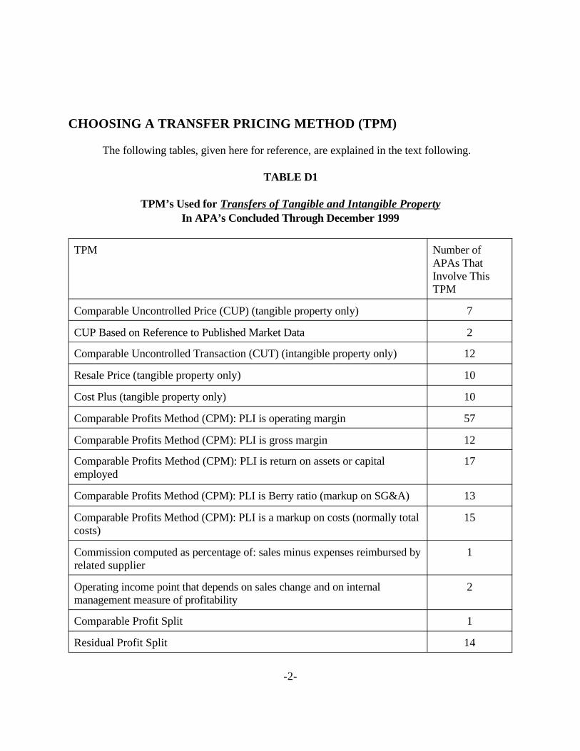
The following tables, given here for reference, are explained in the text following.

TABLE D1

TPM’s Used for Transfers of Tangible and Intangible PropertyIn APA’s Concluded Through December 1999

TPM Number ofAPAs ThatInvolve ThisTPM

Comparable Uncontrolled Price (CUP) (tangible property only) 7

CUP Based on Reference to Published Market Data 2

Comparable Uncontrolled Transaction (CUT) (intangible property only) 12

Resale Price (tangible property only) 10

Cost Plus (tangible property only) 10

Comparable Profits Method (CPM): PLI is operating margin 57

Comparable Profits Method (CPM): PLI is gross margin 12

Comparable Profits Method (CPM): PLI is return on assets or capitalemployed

17

Comparable Profits Method (CPM): PLI is Berry ratio (markup on SG&A) 13

Comparable Profits Method (CPM): PLI is a markup on costs (normally totalcosts)

15

Commission computed as percentage of: sales minus expenses reimbursed byrelated supplier

1

Operating income point that depends on sales change and on internalmanagement measure of profitability

2

Comparable Profit Split 1

Residual Profit Split 14

-3-

For globally integrated commodity trading, profit split by formula based oncompensation and commodity positions

2

Other Profit Split 8

Profit set to sum of a certain return on assets and a certain operating margin;this method combined with an other profit split

1

Agreed royalty (fixed rate) 7

Agreed royalty (rate varies with operating margin) 2

Agreed royalty (rate varies with ratio of R&D to sales) 1

Taxpayer’s worldwide royalty schedule justified by CPM analysis 1

R&D cost sharing amount plus a percentage of sales 1

-4-

TABLE D2

TPM’s Used for ServicesIn APA’s Concluded Through December 1999

TPM Number of APAsThat Involve ThisTPM

Charge-out of cost with no markup 17

Charge-out of cost with markup 41

Commission as percentage of sales 2

Markup on costs, but R&D expenses limited to certain percentage of sales 1

Asset-proportionate share of system-wide return on assets, but limited tocertain range of markup on costs

1

Profit is the sum of a markup on costs, a percentage of sales of patentedproducts resulting from contract R&D performed by tested party, andother factors

1

For real estate management, fee is percentage of rents plus percentage oftotal value of new leases, but not less than a certain markup on costs

1

Dollar cap on management fee 1

Profit split using five-factor formula 1

Profit split, subject to a floor on operating margin 1

-5-

TABLE D3

TPM’s Used for Financial ProductsIn APA’s Concluded Through December 1999


Profit split under Notice 94-40/Prop. Reg. 1.482-8 20

Residual profit split 2

Interbranch allocation (e.g., foreign exchange separate enterprise) 18

Market-based commission 2

Taxpayer’s internal allocation system 1

TABLE D4

TPM’s Used for Contributions to Cost Sharing ArrangementsIn APA’s Concluded Through December 1999

Cost Allocated By Number of APAsUsing ThisAllocation

Sales 7

Sales and production costs 2

Sales and profit 2

Profit 2

Raw material costs 1

-6-

TABLE D5

TPM’s Used for Cost Sharing Buy-in PaymentsIn APA’s Concluded Through December 1999


Capitalized R&D 2

The sum of the two payments, one based on capitalized R&D and the otherbased on residual profit split analysis

2

Market capitalization 1

Residual profit split with comparable acquisitions check 1

Specified Methods

Tables D1- D5 above list the transfer pricing methods (TPMs) used in APAs concludedthrough December1999. In general, the TPMs shown track the methods specified in theRegulations. Reg. § 1.482–3(a) specifies the following methods to determine income withrespect to a transfer of tangible property:

• comparable uncontrolled price (“CUP”) method (Reg. § 1.482–3(b))• resale price method (Reg. § 1.482–3(c))• cost plus method (Reg. § 1.482–3(d))• comparable profits method (“CPM”) (Reg. § 1.482–5)• profit split method (Reg. § 1.482–6).

Reg. § 1.482–4 specifies the following methods to determine income with respect to atransfer of intangible property:

• comparable uncontrolled transaction (“CUT”) method (Reg. § 1.482–4(c))• comparable profits method (“CPM”) (Reg. § 1.482–5)• profit split method (Reg. § 1.482–6)

The Regulations also provide methods applicable to transactions other than the transfer oftangible or intangible property. Reg. § 1.482–2(a) provides rules concerning the propertreatment of loans or advances between controlled taxpayers. Reg. § 1.482–2(b) dealswith provision of services, providing that services ordinarily should bear an arm’s lengthcharge, and that in certain circumstances an arm’s length charge may be deemed to be thecost of providing the services. Finally, Reg. § 1.482–7 provides rules for qualified cost

-7-

sharing arrangements under which the parties agree to share the costs of development ofintangibles in proportion to their shares of reasonably anticipated benefits from their use ofthe intangibles assigned to them under the agreement. APAs dealing with such cost sharingagreements can deal with both the method of allocating costs among the parties, and thedetermination of the amount of the “buy in” payment due when one party to a cost sharingarrangement makes preexisting intangibles available for the benefit of all participants.

Flexible “Best Method” Approach; Unspecified Methods

Under the Regulations, there is no strict hierarchy of methods. Further, particulartransaction types are not assigned exclusively to particular methods. Instead, theRegulations prescribe a more flexible “best method” approach. The best method is themethod that provides the most reliable measure of an arm’s length result. Reg. §1.482–1(c)(1). Moreover, methods not specified in these sections may be used if theyprovide a more reliable result; such methods are referred to as “unspecified methods.”

Usually, data based on results of transactions between unrelated parties provide the mostobjective basis for determining an arm’s length price. Reg. § 1.482–1(c)(2). In suchcases, reliability is a function of the degree of comparability between the controlledtransactions or taxpayers and the uncontrolled comparable transactions or parties, thequality of the data and assumptions used in the analysis, and the sensitivity of the results todeficiencies in the data and assumptions. Reg. § 1.482–1(c)(2). Factors affectingcomparability include the industry involved, the functions performed, the risks assumed,contractual terms, the relevant market and market level, and other considerations. Reg. §1.482–1(d)(3). Moreover, “[i]f there are material differences between the controlled anduncontrolled transactions, adjustments must be made if the effect of such differences onprices or profits can be ascertained with sufficient accuracy to improve the reliability ofthe results.” Reg. § 1.482–1(d)(2).

Thus, one normally cannot say that a TPM in the abstract is the most reliable. Rather, onepicks the most reliable combination of TPM, comparables, and adjustments. TPMs arediscussed in this section, comparable selection in the next section, and adjustments to thecomparables’ data in a later section. However, because these topics are closely linked,concepts about comparables and adjustments will be introduced in this section as needed.

Choosing the best method often requires considerable judgment. The need for judgment results in a large number of controversies between taxpayers and the Service, and is onereason the APA Program was established as an alternative dispute resolution forum. APAcases often are more difficult than a typical transfer pricing case. (If a case is easy toresolve, there is less need to resort to the APA process.) Since the best method is highlyfact specific to a particular case, the APA Team must develop a clear, detailedunderstanding of the taxpayer’s business, including the taxpayer’s functions and risks, theindustry involved, market conditions, and contractual terms. This factual development ismuch easier to accomplish in a cooperative effort with taxpayers than in an adversarialsetting such as audit and litigation.

-8-

The APA process has proven a valuable way for the Service to learn more abouttaxpayers’ businesses, and their concerns and difficulties in attempting voluntarily tocomply with their tax obligations. This experience can enable the Service to providebetter and more timely guidance about TPMs to taxpayers in general (not limited to those inthe APA Program). A good example concerns “global dealing” cases. In these cases, aglobal financial institution or affiliated group of companies would continuously tradesecurities and other financial products on a twenty-four hour basis, with responsibility forthe “book” of positions passing from location to location in accordance with the passing ofnormal business hours in a given location. Existing rules created uncertainty regarding theappropriate treatment of such fact patterns. The Service’s early experience with “globaldealing” APAs was described in Notice 94–40, 1994–1 C.B. 351. This Notice describedthe methods that had been used for a particular type of global dealing case. This Noticeand further APA experience informed the Service’s proposed “global dealing” regulations(63 Fed. Reg. 11177 [REG–208299–90] (March 6, 1998)).

The APA Program’s experience also can help the Office of Associate Chief Counsel(International) to provide better advice about TPMs to the field. An example is that theAPA Program’s experience with cost sharing buy-ins (discussed below) has informed theService’s advice given to the field on some audits of buy-ins.

Some types of TPMs used in APAs are discussed below. First, however, here are somegeneral remarks and concepts.

Creativity

The various TPMs are sometimes used in a creative manner, based on the economiccircumstances and the legitimate concerns of both the Service and the taxpayer. Forexample, if an APA’s TPM features a gross margin target for a U.S. distributor thatpurchases from a related foreign manufacturer, the Service may be concerned aboutexcessive advertising expenses. Indeed, since advertising expenses do not affect grossmargin, a taxpayer could, while staying within the prescribed gross margin range, conducta large advertising campaign that primarily benefits a related foreign manufacturer thatowns the brand name. The advertising would reduce U.S. operating profit and taxableincome, but the benefits of the advertising would rest largely with the foreign parent. Toprevent this situation, an APA could specify that, for purposes of computing thedistributor’s gross margin, advertising expenses above a certain level will be subtractedfrom sales (and thus decrease the gross margin). Then the taxpayer could not freelyincrease advertising expenses while staying within its gross margin range.

As another example, an APA using a CPM might specify a particular gross margin range,but subject to the need to meet a certain operating margin range. (Such a case would havebeen counted in Table D1 above as one instance of a CPM with an gross margin profitlevel indicator (PLI), plus one instance of a CPM with an operating margin PLI.).

Tested Party

-9-

In reviewing the methods discussed below, bear in mind the concept of “tested party.” Controlled transactions must involve two related parties. With some TPMs, only theresults of one of these parties are tested. For instance, consider a parent company thatmanufactures products that it sells to its subsidiary for wholesale distribution. With theresale price method under Reg. § 1.482–3(c), only the distributor’s gross margin is tested. With the cost plus method under Reg. § 1.482–3(d), only the manufacturer’s markup on costof goods sold is tested. With the comparable profits method under Reg. § 1.482–5, oneparty’s profitability (normally that of the simpler party, with no or fewer pertinentintangible assets) is tested. As another example, for provision of services under Reg. §1.482–2(b), typically only the provider of services is tested.

With some TPMs, the prices or results of both parties are tested. For example, with thecomparable uncontrolled price method under Reg. § 1.482–3(b), the price charged betweenthe related parties is tested . Similarly, with the comparable uncontrolled transactionmethod under Reg. § 1.482–4(c), the compensation for intangibles paid between the relatedparties is tested. With profit split methods under Reg. § 1.482–6, and for financialproducts cases under Prop. Reg. § 1.482–8, the split of profits between the related partiesis tested in light of each party’s contributions. With cost sharing under Reg. § 482–7, theparties’ sharing of costs is tested in light of the parties’ reasonably anticipated benefits.

The choice of tested party (together with the choice of TPM) can reflect a choice abouthow to allocate risk. Consider a manufacturer selling to a controlled distributor. Testingonly the distributor (for example, using a CPM with an operating margin PLI) assigns thedistributor a particular profit range. The distributor must then earn a profit within thatrange without regard to the system profit (i.e., the combined profit from manufacturing anddistribution). Thus, the distributor might be guaranteed a certain positive profit level evenwhen the manufacturer is sustaining substantial losses and the system profit is negative. One treaty partner has called this situation “profit creation” since it assigns profit to oneparty despite an overall loss. In particular cases this result may be a correct assignment ofrisk. However, in some cases one could argue for a sharing of risk, for example a profitsplit approach, in which both parties are tested. A profit split approach would lead to less“profit creation” when the system profit is negative and conversely would give thedistributor more profit when the system profit is large.

Transactional Versus Profit-Based Methods

Some TPMs, such as CUP, CUT, resale price, and cost plus, use comparable uncontrolledtransactions to determine an arm’s length price or range of prices. For example, the CUPmethod computes an arm’s length price or range of prices for the transfer of goods basedon a comparable uncontrolled price for the same or similar goods. Such methods arecalled “transactional” methods. Other methods, such as CPM and profit split methods, usecomparable uncontrolled companies to determine appropriate aggregate profit levels forthe tested party. For example, the CPM method specifies a particular profitabilitybenchmark for the tested party. Such methods are called “profit-based” methods. Sometimes a profit-based method is most reliable because closely comparable

-10-

uncontrolled transactional data are not available.

Internal and External Comparables

For transactional methods, one can distinguish “internal” versus “external” comparableuncontrolled transactions. Internal comparables are based on transactions between amember of the controlled group being analyzed and an uncontrolled party. For example, todetermine an arm’s length price or range of prices for a manufacturer M to sell a specificgood to a related distributor D, one might consider either the price that M chargesunrelated distributors for this good, or the price at which D buys this good from unrelatedmanufacturers. External comparables are based on transactions not involving a member ofthe controlled group being analyzed. In the scenario just given, an external comparabletransaction would be a price charged between a manufacturer and distributor who are notrelated to each other and are not members of the controlled group under analysis. Internalcomparables are sometimes preferable to external comparables because (1) more completefinancial data and/or descriptive information may be available, and (2) the internaltransactions may involve circumstances that are more similar to the circumstances of thetransaction being tested.

CUP

The CUP method has been used when one can identify uncontrolled transactions with therequired degree of comparability between products, contractual terms, and economicconditions. See Reg. § 1.482–3(b)(2)(ii). If the covered product is a commodity, thenpublicly available market data may provide a comparable price that could be used toestablish a CUP. In many other cases, however, data concerning external CUPs is difficultto obtain. Unrelated taxpayers dealing in the comparable product ordinarily would alsodeal in other items as well, and it is sometimes difficult to separate the pricing of therelevant transactions from the other results, based on publicly available data. Thus, in theAPA Program’s experience, there has been a tendency to use internal CUPs.

CUT

A CUT is a CUP for transfers of intangible property. As with the CUP method, APAsapplying the CUT method have tended to rely on internal transactions between the taxpayerand unrelated parties since it has often been difficult to identify an external CUT. Forexample, in a case dealing with a royalty for a nonroutine intangible such as a trademark, itcan be difficult to identify an unrelated party royalty arrangement that is sufficientlycomparable, due to the unique nature of the nonroutine intangibles. (Lesson 2 [not yetwritten] discusses how to determine arm’s length royalty rates.)

Resale Price and Cost Plus

As of December 31, 1999, ten APAs had used a transactional resale price method, andanother ten had used a transactional cost plus method. As with the CUP and CUT

-11-

approaches, internal comparables tend to be more reliable than external comparables. However, because product similarity is less important for the resale price and cost plusmethods than for the CUP method (see Reg. § 1.482–3(c)(3)(ii)(B), –3(d)(3)(ii)(B)),external comparables in many cases can be used.

It is sometimes hard to distinguish a transactional resale price method from a CPM with agross margin PLI (discussed below), and to distinguish a transactional cost plus pricemethod from a CPM with a markup on cost of goods as the PLI (discussed below). Thedifference in both cases is one of degree rather than kind. A transactional method focuseson prices for individual or narrow groups of transactions, while a CPM looks at profitsfrom broader groups of transactions or all of a company’s transactions. When dealing withtreaty partners that do not favor a CPM approach, it sometimes helps to use the term“resale price” or “cost plus” rather than “CPM”.

CPM

The CPM is frequently applied in APAs. Reliable public data on comparable businessactivities of independent companies is often more readily available than potential CUPdata. Also, comparability of resources employed, functions, risks, and other importantconsiderations for the CPM method is more likely to exist than the comparability ofproduct that is important for the CUP method.

The CPM is most commonly used with a profit level indicator, or PLI (defined below),such as operating margin or return on assets, that is based on operating profit. In suchcases, the CPM does not require comparability between the tested party and thecomparables regarding the classification of expenses as cost of goods sold or operatingexpenses, since that classification does not affect operating profit. The cost plus and resaleprice methods, in contrast, depend on such comparability. Reg. §§ 1.482-5(c)(3)(ii),1.482–3(c)(3)(iii)(B), 1.482–3(d)(3)(iii)(B). Also, in such cases the degree of functionalcomparability required to obtain a reliable result under the CPM is generally less than thatrequired under the resale price or cost plus methods. Because differences in functionsperformed often are reflected in operating expenses, taxpayers performing differentfunctions may have very different gross profit margins but earn similar levels of operatingprofit. Reg. § 1.482–5(c)(2)(ii).

As can be seen from Table D6, several profit level indicators (“PLIs”) have been usedwith the CPM. A PLI is a measure of a company’s profitability that is used to comparecomparables with the tested party. The regulations specifically mention only return onassets, operating margin, and Berry ratio, but state that other PLIs “may be used if theyprovide reliable measures” of arm’s length results. Reg. 1.482-5(b)(4). The choice of PLIturns on all the factors contained in the Regulations, including availability and reliability ofinformation, and the nature of the tested party’s activities.

1The regulations use the term “return on capital employed” for this PLI. That term can beabbreviated as “ROCE”. The APA Program uses ROCE as a synonym for ROA. However, somepractitioners use ROCE as a synonym for ROIC, on the next line of this table.

2The regulations use the term “operating assets,” which is defined in Reg. § 1.482-5(d)(6). This definition does not exclude intangible property. However, the APA Program normallyexcludes intangible property for reasons discussed below and then, to be consistent, excludesamortization of intangible property from the calculation of operating profit.

3Named after Professor Charles Berry, who used the Berry ratio when serving as an expertwitness in E.I. DuPont de Nemours & Co. v. United States, 608 F.2d 445 (Ct.Cl. 1979). Theregulations do not use the term “Berry ratio,” but the term is widely used in practice.

4Operating expenses means selling, general, and administrative, expenses, includingdepreciation. This is consistent with the definition in Reg. § 1.482-5(d)(4).

Since gross profit equals operating profit plus operating expenses, the definition of Berryratio given above is equivalent to the sum of operating profit and operating expenses, all dividedby operating expenses; this in turn is equivalent to 1 plus the ratio of operating profit to operatingexpenses. Therefore, if the company has positive profits the Berry ratio is greater than one.

5Total costs, which equals cost of goods sold plus operating expenses, is sometimesreferred to as “fully loaded costs.”

-12-

TABLE D6Profit Level Indicators (PLIs)

PLI Definition

return on assets (ROA)1 operating profit divided by the value of assets (normally, onlytangible assets) actively employed in the business2

return on invested capital(ROIC)

operating profit divided by the following: the value of assets(normally, only tangible assets) actively employed in thebusiness, minus non-interest bearing liabilities (NIBLs) suchas accounts payable

operating margin (OM) operating profit divided by sales

gross margin (GM) gross profit divided by sales

Berry ratio3 gross profit divided by operating expenses4

markup on total costs operating profit divided by total costs5

markup on cost of goods sold gross profit divided by cost of goods sold

6Reg. §§ 1.482-5(b)(4)(1), 1.482-5(d)(6). (This definition applies only to ROA; theregulations do not mention ROIC.) Also, the regulations mandate using the average of thebeginning and end of year asset levels “unless substantial fluctuations . . . make this an inaccuratemeasure of the average value over the year,” in which case a more accurate measure of thataverage value must be used. Reg. § 1.482-5(d)(6).

-13-

The first two PLIs listed divide operating profit by a balance sheet figure. The definitionof each balance sheet figure is based on tangible assets actively employed in the business. This consists of all assets, minus intangible assets such as goodwill, minus investments(e.g., in subsidiaries), minus excess cash and cash equivalents (e.g., cash and cashequivalents beyond the amount needed for working capital). (Practitioners sometimes useslightly different definitions.) The regulations instead use the term “operating assets” andin turn define that term.6 While the regulations allow for measuring all companies’ assetson a consistent basis in terms of either book or fair market value, in the APA Program’sexperience one cannot get the fair market value of assets for all companies. Also, whilethe definition in the regulations may leave intangible assets in the asset base, in the APAProgram’s experience it is difficult to include the tested party’s and the comparables’intangibles on a consistent basis. For example, intangibles acquired through purchasenormally are listed on a company’s books but intangibles developed internally are not. Therefore, the APA Program normally leaves intangibles out of the asset base. To beconsistent, the APA Program then excludes amortization of intangible property from thecalculation of operating profit. (That is, such amortization is not counted as an operatingexpense.)

This type of PLI may be most reliable if the level of tangible operating assets has a highcorrelation to profitability. Reg. § 1.482–5(b)(4)(i). For example, a manufacturer’soperating assets such as property, plant, and equipment could have more impact onprofitability than a distributor’s operating assets, since often the primary value added by adistributor is based on services it provides, which are often less dependent on the level ofoperating assets. The reliability of this type of PLI can also depend on the structure of thetaxpayer’s tangible assets and their similarity to those of the comparables, since differentasset categories can have different rates of return. (For example, fixed assets may be morerisky than accounts receivable and thus command a higher return.) The reliability also canbe diminished if the comparables vary substantially from the tested party in their relativeamounts of tangible and intangible assets, since intangible assets are left out of the assetbase but contribute to profitability. Finally, the reliability can be diminished if there areproblems in using book values as a proxy for the fair market values of tangible assets. Forexample, a company may have facilities that show a very low book value because ofdepreciation but in fact are still substantially productive.

The difference between ROA anc ROIC is that ROA focuses on the assets used, whileROIC focuses on the amount of debt and equity capital that is invested in the company. Consider two companies that each have operating assets totaling $200. Suppose the firstcompany has no non-interest-bearing liabilities (NIBLs), and the second company has $100of NIBLs in the form of accounts payable. Both have operating assets (the denominator for

-14-

the ROA PLI) of $200. However, when it comes to invested capital (the denominator forthe ROIC PLI), the first company has $200 while the second company has $100. The firstcompany requires $200 in debt and equity financing; the second requires only $100, sinceits suppliers are providing the other $100 needed to run the business. As discussed later inconnection with asset intensity adjustments, many economists who use ROA make anadjustment for NIBLs such as accounts payable, which narrows the differences in resultsachieved using ROA and ROIC.

Other PLIs consist of ratios between income statement items. These include operatingmargin (“OM”), gross margin (“GM”), Berry ratio, markup on total costs, and markup oncost of goods sold. For technical reasons, the denominator in the PLI’s definition generallyshould be an item that does not reflect controlled transactions. Thus, the operating marginand gross margin PLIs (which have sales in the denominator) generally are used for testedparties (often distributors) that sell to unrelated parties, while the markup on costs PLIs(which have total costs or cost of goods sold in the denominator) generally are used fortested parties (often manufacturers) that buy from unrelated parties. The Berry ratio PLI,which has operating expenses in the denominator, in principle could be used in either case.

PLIs based on income statement items are often used when fixed assets do not play acentral role in generating operating profits. This is often the case for wholesaledistributors and for service providers. Also, income statement-based PLIs may be morereliable when balance-sheet-based PLIs are unreliable for reasons discussed above. Forexample, consider a wholesale distributor tested party and wholesale distributorcomparables that each perform a significant marketing function and hold significantmarketing intangibles. Suppose that compared to the comparables, the tested party holdsrelatively little inventory and extends relatively little credit to its customers. Then thetested party’s ratio of intangible to tangible assets may be substantially greater than thecomparables’ ratios; as discussed above, in such circumstances balance-sheet-based PLIsare less reliable. The tested party’s intangible asset to sales ratio might however besimilar to comparables’ ratios. For example, each company may have dealer networks thathave value in proportion to sales. Then each company’s intangibles would contributeabout the same amount to the operating margin, so that an operating margin PLI might bereliable.

Operating margin has often been used when functions of the tested party are not closelymatched with those of the available comparables, since differences in function have lesseffect on operating profit than on some other measures such as gross profit (see Reg. §1.482-5(c)(2)(ii)).

Conceptually, the Berry ratio represents a return on a company’s value added functions andassumes that the company’s value added functions are captured in its operating expenses. This assumption is more reliable for distributors than for manufacturers. Formanufacturers, much of the value added function is reflected in cost of goods sold. Severalempirical studies performed by taxpayers and Service economists suggest that uncontrolledwholesale distributors with relatively low operating expense to sales levels (i.e., below

7Operating margin and markup on total costs have a mathematical relationship such that onecan compute one from the other. Let OM and MTC denote operating margin and markup on totalcosts, respectively. Let S, P, and C denote sales, operating profit, and total costs, respectively, sothat S = P+C. Then OM is defined as P/S and MTC is defined as P/C. Then MTC = P/C = P/(S-P) = (P/S)/((S/S)-(P/S)) = OM/(1-OM). Similarly, OM = P/S = P/(C+P) = (P/C)/((C/C+(P/C)) =MTC/(1+MTC).

-15-

10 to 15 percent) report much higher Berry ratios than companies with higher operatingexpense to sales levels. This result suggests caution in using the Berry ratio PLI tocompare companies with low operating expense to sales ratios to companies with higheroperating expense to sales ratios. On the other hand, the Berry ratio may be preferable tooperating margin if variations in sales volume do not involve similar variations in functionand risk. The following subsection discusses one such situation involving commissionagent activity.

In general, gross margin has not been favored as a PLI because the categorization ofexpenses as operating expenses or cost of goods sold may be subject to manipulation, sothat a taxpayer generating significant operating losses could nevertheless show grossmargins within an arm’s length range defined by a set of comparables with high operatingprofits. Further, as mentioned, functional differences can make a gross margin PLIunreliable.

As mentioned above, for technical reasons, the PLI’s denominator generally should notreflect controlled transactions. Therefore, one may consider using a markup on total costsrather than an operating margin when total costs reflects controlled transactions but salesdo not.7 An example is testing a manufacturer that sells to a controlled distributor. Occasionally, a PLI has been used that consists of operating profit divided by some subsetof total costs. In one case, for example, product specific taxes reimbursed by the purchaserwere excluded from the cost pool considered. Also, occasionally markup on cost of goodssold has been used as the PLI. That PLI shares the disadvantages of the gross margin PLI,discussed in the previous paragraph.

The choice of PLI is often a substantial issue in APA negotiations. The choice of PLIdepends on the facts and circumstances of a particular case. The APA Team’s analysisoften will consider multiple PLIs. If the results tend to converge, that may provideadditional assurance that the result is reliable. If there is a broad divergence between thedifferent PLIs, the Team may derive insight into important functional or structuraldifferences between the tested party and the comparables. For example, such divergencemay lead to a discovery that the taxpayer’s indicated asset values are not reliable orcomparable, such as in the case of a largely depreciated but still valuable asset base.

Commission Income

Sometimes taxpayers propose using the CPM when the tested party and the comparables

8Sometimes one hears the term “commissionaire.” Like a commission agent, acommissionaire facilitates direct sales from the supplier to the customer and gets paid acommission by the supplier. However, a commissionaire offers goods under its own name, whilea commission agent offers goods under the supplier’s name. In common law countries acommissionaire is considered an undisclosed agent and binds the supplier. In civil law countriesa commissionaire is not considered the supplier’s agent and thus does not bind the supplier. Michael Swanick, Mark Mudrick, and Erik Bouwman, “Tax and Practical Issues inCommissionaire Structures,” 97 TNT 17-63 (Tax Analysts). The analysis in this subsectionapplies to commissionaires as well as commission agents since both in general have lessfunctionality, assets, and/or risk than distributors.

9Some companies with mixed activity report commission income as a contra to operatingexpenses rather than as a revenue item. In such cases, one normally should restate commissionincome as a revenue item for purposes of the TPM.

10However, this expectation might not always come true. If a distributor’s risks turned outbadly and had an adverse effect on its financial results, one might after-the-fact expect the

-16-

have different proportions of commission sales. A Team Leader should exercise duediligence to identify these situations because they may require special treatment. In thesesituations an operating margin PLI can be problematic. The reason, explained below, isthat given the revenues, functions, risks, and assets of commission sales activity, there is noreason to think that commission sales and ordinary distribution of the same products in thesame market result in the same arm’s length operating margin.

While a distributor buys items from a manufacturer or other supplier and then resells themto the customer, a commission agent8 facilitates direct sales from the supplier to thecustomer and receives a commission payment for its services. (The commission is oftencomputed as a percentage of the price paid by the customer.) Sometimes a party does bothdistribution and commission sales. While a distributor reports revenue as the dollaramount of the product sold to customers (third-party sales), a commission agent generallyreports revenue as the dollar amount of commission received from the supplier, which isoften a small fraction of the third party sales.9

It is helpful to think of a commission agent as a somewhat stripped-down or reduceddistributor. A commission agent normally performs somewhat less functionality than adistributor. For example, a commission agent might not find customers, or might notwarehouse goods. A commission agent also typically incurs somewhat less risk than adistributor. For example, since it does not take title to goods, it typically has lessinventory risk. A commission agent also typically requires somewhat less assets than adistributor. For example, since it does not take title to the goods, a commission agentwould not have an inventory asset for those goods; and it might lack other assets such aswarehouses. The extent of these differences can vary. At one extreme, a commission agentmight look exactly like a distributor (e.g., finds customers, warehouses goods) except thatit does not take title to the goods. At the other extreme, the supplier might find customersand directly ship goods to the customer, with the commission agent performing only someminor functions such as billing or minor customer support. Because of this reducedfunctionality, risk, and assets, a commission agent typically would expect to earn lessoperating profit than a distributor per product sold or per dollar of third-party sales.10

commission agent to have more operating profit than a distributor per product sold or per dollar ofthird-party sales.

-17-

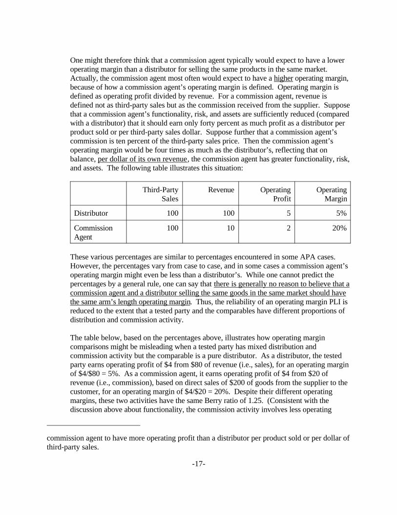
One might therefore think that a commission agent typically would expect to have a loweroperating margin than a distributor for selling the same products in the same market. Actually, the commission agent most often would expect to have a higher operating margin,because of how a commission agent’s operating margin is defined. Operating margin isdefined as operating profit divided by revenue. For a commission agent, revenue isdefined not as third-party sales but as the commission received from the supplier. Supposethat a commission agent’s functionality, risk, and assets are sufficiently reduced (comparedwith a distributor) that it should earn only forty percent as much profit as a distributor perproduct sold or per third-party sales dollar. Suppose further that a commission agent’scommission is ten percent of the third-party sales price. Then the commission agent’soperating margin would be four times as much as the distributor’s, reflecting that onbalance, per dollar of its own revenue, the commission agent has greater functionality, risk,and assets. The following table illustrates this situation:

Third-PartySales

Revenue OperatingProfit

OperatingMargin

Distributor 100 100 5 5%

CommissionAgent

100 10 2 20%

These various percentages are similar to percentages encountered in some APA cases. However, the percentages vary from case to case, and in some cases a commission agent’soperating margin might even be less than a distributor’s. While one cannot predict thepercentages by a general rule, one can say that there is generally no reason to believe that acommission agent and a distributor selling the same goods in the same market should havethe same arm’s length operating margin. Thus, the reliability of an operating margin PLI isreduced to the extent that a tested party and the comparables have different proportions ofdistribution and commission activity.

The table below, based on the percentages above, illustrates how operating margincomparisons might be misleading when a tested party has mixed distribution andcommission activity but the comparable is a pure distributor. As a distributor, the testedparty earns operating profit of $4 from $80 of revenue (i.e., sales), for an operating marginof $4/$80 = 5%. As a commission agent, it earns operating profit of $4 from $20 ofrevenue (i.e., commission), based on direct sales of $200 of goods from the supplier to thecustomer, for an operating margin of $4/$20 = 20%. Despite their different operatingmargins, these two activities have the same Berry ratio of 1.25. (Consistent with thediscussion above about functionality, the commission activity involves less operating

11Asset intensity adjustments probably would narrow this difference. As suggested above,the commission activity likely has a higher asset-to-revenue ratio than the distribution activity. Insuch cases, asset intensity adjustments would either lower the tested party’s operating margin orraise the comparable’s operating margin before the two are compared. However, in general it isdifficult to determine to what extent asset intensity adjustments correct this difference, so thatrelying on such adjustments may not be the most reliable method.

12A fourth alternative might be to use an operating margin PLI on the tested party’scombined operations but to alter the calculation by “grossing up” the commission income to thedollar amount of the third-party sales. However, this alternative is problematic. To follow this

-18-

expense per third-party sales than the distribution activity, but involves more operatingexpense per booked revenue than the distribution activity.) For purposes of this example,assume that both activities of the tested party earn an arm’s length return.

Tested Party,Total

Tested Party,Commission

Segment

Tested Party,Distributor

Segment

UncontrolledDistributor

Third-Party Sales 280 200 80 80

Revenue 100 20 80 80

Cost of Goods Sold 60 0 60 60

Operating Expense 32 16 16 16

Operating Profit 8 4 4 4

Operating Margin 8% 20% 5% 5%

Berry Ratio 1.25 1.25 1.25 1.25

Suppose next that the taxpayer finds an uncontrolled company that acts only as a distributor(no commission sales), with an income statement identical to that for the tested party’sdistribution activity. Suppose further that the taxpayer proposes using the CPM with anoperating margin PLI to test the tested party’s combined activities. The uncontrolleddistributor’s operating margin is 5%. The tested party’s distribution operations also havean operating margin of 5%, but the tested party’s combined operations have an operatingmargin of 8%, which might lead one to erroneously conclude that the tested party hasearned too much profit.11

To avoid this situation, one could either (1) use a different PLI such as the Berry ratio, (2)separately test the tested party’s distribution and commission operations, or (3) test onlythe tested party’s distribution operations and exclude the commission operations from theAPA’s covered transactions.12

alternative in the example above, one would substitute sales of $200 for the commission income of$20. The tested party’s combined operating margin would then be computed as 8/(80+200) =8/280 = 2.9%, which might suggest that the tested party is earning too little compared to theuncontrolled distributor’s operating margin of 5%. However, this suggestion would be flawed. Indeed, as discussed above, one normally would expect a commission agent to earn less operatingprofit per third-party sales than a distributor because the commission agent normally has lessfunctionality, risk, and assets per dollar of third-party sales. If a gross-up approach is used, oneprobably should perform a further adjustment to reflect these differences. This further adjustmentmight in some cases be accomplished in whole or in part through asset intensity adjustments. Because a commission agent typically has less assets than a distributor per dollar of third-partysales, asset intensity adjustments typically would raise the tested party’s operating margin orlower the uncontrolled distributor’s operating margin before the two are compared. However, ingeneral it is difficult to determine to what extent asset intensity adjustments correct this difference,so that relying on such adjustments may not be the most reliable method.

13This subsection has stressed the pitfalls of using on operating margin PLI whencommission income is involved. However, some practitioners believe that in most cases testingdistribution and commission activity together with an operating margin PLI actually will producecorrect results, in light of the rules on aggregation and set-off (Reg. §§ 1.482-1(f)(2)(i), -1(g)(4)),the safe harbor for nonintegral services (Reg. § 1.482-2(b)), the possibility that comparables mayhave a similar mix of activity, and the business realities of commission income. Henry Birnkrantand Pamela Ammermann, “A Dissenting View on the Proper Application of §482 to a Distributor’sCommission Income”, 30 Tax Management International Journal 539 (Dec. 7, 2001).

-19-

A taxpayer requesting an APA should explain the extent to which the tested party and thecomparables have a different mix of distribution and commission income, and should takesuch differences into account in the proposed TPM. If the Taxpayer’s request is not clear,the Team Leader will need to clarify this point before agreeing on a TPM.13

Hybrid PLI

In some cases, one PLI can be transformed into another PLI. The result is a hybridcombining some features of each. The most common example is transforming an operatingmargin into a gross margin. This happens as follows. First, the comparables’ operatingmargins are computed for the analysis window. (Analysis windows are discussed in alater section.) Next, the tested party’s operating expenses as a percentage of sales areadded to each comparable’s operating margin, to compute what the comparable’s grossmargin would have been if the comparable had had the same level of operating expenses asthe tested party. These “constructed” gross margins of the comparables are used todetermine a gross margin range for the tested party for the APA years. (In Table D6, thisapproach would be counted as using a gross margin PLI, since the TPM specifies a grossmargin range for the tested party to meet during the APA years.)

14A taxpayer’s assignment of risks normally should be honored unless it lacks economicsubstance. Reg. 1.482-1(f)(2)(ii)(A) (“In general, the district director will evaluate the results ofa transaction as actually structured by the taxpayer unless its structure lacks economic substance”);Reg. § 1.482-1(d)(3)(iii)(B).

-20-

Why is this hybrid approach used? In the example just given, the taxpayer or treaty partnermay want to use a gross margin PLI. For example, a taxpayer may want to use a grossmargin PLI in order to assign more risk to the tested party than an operating margin PLIwould14 or to give the tested party more incentive to control operating expenses. Asanother example, a treaty partner might in general object to an operating margin PLI basedon its domestic law or on certain philosophical grounds (e.g., objection to guaranteeing oneparty a particular operating profit even if the other party sustains substantial losses). Yet itmay not be reliable to use the comparables’ gross margins. For example, there may bequestions about whether the comparables categorize expenditures as cost of goods soldversus operating expenses in the same way the tested party does. Also, the tested partymay perform greater functions (as reflected in a higher operating expense level) and thusneed a greater gross margin than the comparables. Backing into a gross margin avoidsthese issues. One uses the comparables’ operating margin, so that there is no issue abouthow the comparables classify expenditures between cost of goods sold and operatingexpenses. Also, adding in the tested party’s operating expenses implicitly adjusts the grossmargin to take into account different levels of functionality.

One can present the approach in this example as using a “gross margin” PLI to appeal totreaty partners averse to the operating margin PLI. One can even present it as a “modifiedresale price” method to appeal to treaty partners that prefer transactional methods to profit-based methods such as the CPM. (Recall that, as discussed above, it can be hard todistinguish a transactional resale price method from a CPM method using a gross marginPLI.)

The hybrid approach has variant forms. In the example just discussed, we transformed anoperating margin range into a gross margin range by adding the tested party’s operatingexpenses during the analysis window to the comparables’ operating margins during theanalysis window. What if instead of adding in the tested party’s operating expenses duringthe analysis window, one added in the tested party’s operating expenses during each APAyear to derive to gross margin range for that APA year? The TPM, while nominally stillusing a gross margin, would then mathematically amount to just an operating margin rangebased on the comparables’ operating margins. Even if one labeled this approach a“modified resale price” method, it might not be palatable to a treaty partner averse to theCPM or to the operating margin PLI. As an intermediate approach, one could derive agross margin range for each APA year by adding in the tested party’s average operatingexpenses over the last few years (perhaps three years). The TPM, still nominally using agross margin, would now in substance use something in between a gross margin andoperating margin PLI.

15There is some question about how to treat intangible development expenses in thiscalculation. This issue is developed in the discussion below of the residual profit split method ofvaluing cost sharing buy-ins.

-21-

Profit Split

Profit split methods are used most often when both sides of the controlled transactions ownvaluable “nonroutine intangibles,” meaning intangibles for which there are no reliablecomparables. If all valuable nonroutine intangibles were owned by only one side, theother side’s contributions could be reliably benchmarked.

The choice between a profit split approach and an approach that assigns one party only areturn for routine functions often represents a choice of how to view the relationshipbetween two related entities. Assigning a party only a routine return implies viewing thatparty as a mere service provider; a profit split, in contrast, implies viewing that party as arisk-taking entrepreneur or joint venture partner. Normally, the parties’ own definition oftheir relationship should be accepted unless it is inconsistent with their conduct and theeconomic substance of the transactions. Reg. § 1.482-1(d)(3)(iii)(B).

In the bilateral context, a profit split approach sometimes makes agreement easier becauseeach country, by sharing in nonroutine profits, can feel that it is getting a “piece of theaction.” Also, a treaty partner might favor a profit split approach in order to avoid “profitcreation” (see the discussion of Tested Party earlier in this section on TPMs). Sometimestreaty partners seek a profit split when the Service believes that the foreign entity shouldget only a routine profit. In some of these cases, the Service has accepted a profit splitapproach as the only way to settle the case.

APAs have used both residual profit splits and (very rarely) comparable profit splits, asdescribed in the Regulations. Under a comparable profit split, the controlled parties’ totalprofits are split in the same ratio as total profits are split between “uncontrolled partiesengaged in similar activities under similar circumstances.” Reg. § 1.482-6(c)(2). Comparable profit splits are generally difficult to apply because of the difficulty of findinguncontrolled parties with sufficiently similar intangibles and circumstances. Only oneAPA has used a comparable profit split.

Under a residual profit split, the controlled parties are first each assigned a routine returnbased on a CPM analysis. Any remaining system profit or loss15 is considered due tononroutine intangibles (i.e., intangibles beyond those possessed by the comparablecompanies used in the CPM analysis) and is split between the parties “based upon therelative value of their contributions of intangible property to the relevant business activitythat was not accounted for as a routine contribution.” Reg. § 1.482-6(c)(3). These relativevalues might be computed according to the ratio of each party’s “capitalized cost ofdeveloping the intangibles and all related improvements and updates, less an appropriateamount of amortization based on the useful life of each intangible.” Id. If these

-22-

expenditures of the parties are “relatively constant over time” and the useful life of theintangible property of all parties is “approximately the same,” then the “amount of actualexpenditures in recent years may be used to estimate the relative value of intangiblecontributions.” Id.

In addition, APAs have used as an unspecified method other types of profit splits. Profitshave been split using weighted allocation formulas reflecting factors intended to reflect therelative contributions of each party. Some APAs have used factors based on operatingassets and certain operating expenses. Some APAs have used factors described in Notice94-40, discussed below under “TPMs for Financial Products Cases.” (While Notice 94-40 was written to cover certain financial products cases, the factors discussed there havebeen used in non-financial-products cases as well.)

TPMs for Financial Products Cases

Various TPMs have been used for financial products cases. One type of financial productscase involves “global dealing,” in which a global financial institution or affiliated group ofcompanies would continuously trade securities and other financial products on a twenty-four hour basis, with responsibility for the “book” of positions passing from location tolocation in accordance with the passing of normal business hours in a given location. These cases have been handled as follows:

• As described in Notice 94–40 (1994–1 C.B. 351), many of these APAs have usedan overall profit split using a multi-factor formula to represent the contribution ofvarious functions to worldwide profits. The factors used have sometimes beencompensation (intended to represent value from highly skilled personnel), tradingvolume (intended to represent level of activity), and maturity-weighted tradingvolume (intended to represent investment risk).

• Residual profit splits, as provided in Prop. Reg. § 1.482–8(e)(6), have beenapplied in two cases where routine functions, such as back office functions, werereadily valued. The residual profits were allocated on the basis of a case specificmulti-factor formula similar to that discussed in Notice 94–40.

• In one case the APA Team determined that the taxpayer’s internal profit allocationmethod provided an arm’s length result. In this case, reliability was enhancedbecause this internal method was used in determining arm’s length payments suchas compensation and bonuses. (See Prop. Reg. 1.482–8(e)(5)(iii).)

• In two cases, where all the intangibles were held in one jurisdiction and the otherjurisdictions provided routine marketing functions, a market based transactionalcommission was used as the most reliable measure of an arm’s length return forthose routine services. (This approach differs from the ones above in that it is not aprofit split. The TPM specifies just a return for routine functions, and onejurisdiction retains all additional profit.)

16The OECD Transfer Pricing Guidelines refer to these arrangements as cost contributionarrangements and discuss them in chapter 8.

17Reg. § 1.482-7(a)(1) states that even if the taxpayer does not comply with therequirements of a qualified CSA then the district director may apply the cost sharing rules to anyagreement that in substance constitutes a CSA.

-23-

A separate group of financial products cases involves U.S. or foreign branches of a singletaxpayer corporation that operate autonomously with respect to the covered transactions. For example, the different branches might autonomously enter into foreign currencytransactions with customers. Pursuant to the business profits articles of the relevantincome tax treaties, several APAs determined the appropriate amount of profits attributableto each branch by reference to the branches’ internal accounting methods. The branchresults took into account all trades, including interbranch and/or inter-desk trades. In orderfor this method to provide a reliable result, however, it was necessary to ensure that allsuch controlled trades be priced on the same market basis as uncontrolled trades. To testwhether this was so, the branch’s controlled trades were matched with that branch’scomparable uncontrolled trades made at times close to the controlled trades. A statisticaltest would then be performed to detect pricing bias, by which the controlled trades might asa whole be priced higher or lower than the uncontrolled trades. See the discussion under“Constructing a Range of Arm’s Length Results” below.

Cost Sharing and Buy-Ins

Some APA cases involve a cost sharing arrangement (“CSA”) under Reg. § 1.482–7.16 Under a CSA, a group of related taxpayers can share in the costs of developing intangiblesthat will be jointly owned. For example, affiliates in the United States, France, and Japanmight share in the costs of developing technology that each affiliate will exploit in itsrespective regional market. A CSA generally obviates the need for royalties for thetechnology developed under the CSA because generally each member of the CSA willexploit only the interests in that technology that it owns (e.g., intangible rights in its ownterritory). To receive this treatment the taxpayer needs to have a “qualified” CSA. Ataxpayer may claim that it has a “qualified” CSA only if it satisfies various requirementsset out in Reg. § 1.482-7(b).17 An APA Team sometimes can work with a taxpayer toensure that these requirements are satisfied. One key requirement is that participants sharecosts of development in proportion to their shares of reasonably anticipated benefits fromexploitation of the intangible to be developed. The regulations contain complex provisionson when and how to prospectively or retroactively adjust the cost shares during the life ofthe CSA based on changed circumstances or incorrect estimation of benefit shares. (Theretroactive adjustment provisions of Reg. § 1.482-7(f)(3)(iv) somewhat resemble theperiodic adjustment provisions of Reg. § 1.482-4(f)(2).) Table D9 shows the methods ofallocating cost sharing payments adopted in APAs completed through December 1999.

18Exhibit E provides legal background on buy-ins.

19Reg. § 1.482-4(c) provides for using comparable uncontrolled transactions of intangibleproperty (“CUT”), involving either “the same intangible property” or “comparable intangibleproperty.” Typically, all participants in a cost sharing arrangement are controlled, and theintangibles supplied are not made available to any party outside the cost sharing group, so that the“same intangible property” approach cannot be used. Taxpayers sometimes propose CUTs basedon “comparable intangible property,” but the very existence of the CSA might make thecircumstances of proposed CUTs not comparable to the circumstances of the tested transaction. (The “existence and extent of any collateral transactions or ongoing business relationships betweenthe transferee and transferor” can affect comparability. Reg. § 1.482-4(c)(2)(iii)(B)(2)(vii).) While a buy-in should compensate the use of preexisting intangibles for further R&D, it is rare thatCUTs confer rights of further development to the licensee. Furthermore, the CUT methods offeredby taxpayers often only provide an initial royalty rate. It may be appropriate to decrease thisinitial royalty rate over time due to the replacement of the preexisting intangibles with theintangibles developed under the CSA. The rate of decline is not addressed in the regulations thatdeal with CUTs. Also, if the intangible transfer occurs before the technology is commercialized,the “comparable intangible property” approach normally cannot be used. Comparability ofintangibles is especially hard to determine at the precommercial stage, and potential comparabletransactions likely would be secret. While the CUT method as presented in Reg. § 1.482-4(c) isthus often not applicable to buy-ins, some buy-in methods discussed below are in part based on aCUT approach. Additionally, a CUT analysis forms the foundation for the market capitalizationmethod.

Reg. § 1.482-5 (Comparable Profits Method (“CPM”)) applies to intangible transfers asfollows. A royalty paid for intangibles is deemed to be arm’s length only if the company payingthe royalty is left with an after-royalty profit that is arm’s length as determined by the CPM. Inprinciple, this approach could apply to determine the buy-in as a royalty stream. However, thecompany paying the royalties for the preexisting intangibles would also be an owner of intangiblesdeveloped under the cost sharing arrangement, and it normally would be difficult to finduncontrolled companies with comparable intangibles upon which to base the CPM analysis. While

-24-

The most difficult CSA cases to resolve are generally those that involve the transfer ofexisting intangibles. For example, one controlled participant might make its ownpreexisting intangibles available to the CSA. That participant is then considered to havetransferred interests in those intangibles to the other controlled participants, which mustpay an arm’s length compensation, or “buy-in” payment. Reg. §§ 1.482–7(a)(2),1.482–7(g)(1),(2).18 Specifically, each other controlled participant must pay the value ofthe CSA’s use of the intangibles at issue, determined according to the rules of § 1.482-1, -4, -5, and -6, multiplied by that participant’s share of reasonably anticipated benefits underthe CSA as defined in § 1.482-7(f)(3). See § 1.482-7(g)(2). For the first step in thiscalculation, the value of the CSA’s use of the intangibles, most of the specified methods forvaluing intangible transfers normally cannot be applied in a straightforward manner in thebuy-in context.19 Some other methods have been developed specially for buy-ins. In some

the CPM presented in Reg. § 1.482-5 is thus not often applicable to buy-ins, some buy-in methodsdiscussed below are in part based on a CPM approach.

Another specified method is the comparable profit split under Reg. § 1.482-6(c)(3). Asdiscussed above, this method is only rarely useable. Applying a comparable profit split to a costsharing buy-in would be especially difficult because “comparability under this method alsodepends particularly on the degree of similarity of the contractual terms of the controlled anduncontrolled taxpayers.” One rarely finds uncontrolled taxpayers in a similar cost sharingarrangement.

-25-

cases, these methods are based in part on specified methods such as CUT and CPM. Thesevarious methods are discussed later.

Buy-in payments may take the form of a lump sum payment, a series of installmentpayments based on a lump sum up front value with arm’s length interest, or “royalties orother payments contingent on the use of the intangible by the transferee.” Reg. § 1.482-7(g)(7). On audit, the taxpayer is normally free to choose the form of payment unless itsarrangement lacks economic substance. See Reg. § 1.482-1(f)(2)(ii)(A) (“The districtdirector will evaluate the results of a transaction as actually structured by the taxpayerunless its structure lacks economic substance.”) In the APA context, the Service mightargue for its preferred form of payment as part of the give-and-take of negotiations. Someof the buy-in methods discussed below naturally yield a lump sum result, while othersnaturally yield a result as a stream of royalties. If the best method yields a lump sum butthe taxpayer has chosen a royalty stream, the lump sum can be converted (with the help ofan economist and some assumptions) into a royalty stream. Similarly, if the best methodyields a royalty stream but the taxpayer has chosen a lump sum, the royalties can beconverted (again with the help of an economist and some assumptions) into a lump sum. Inpractice, taxpayers tend to choose royalty streams.

Table D5 shows buy-in methods used in APAs completed through December 1999. Thesemethods have been adopted on a case by case basis, depending on the taxpayer’s facts andcircumstances. Most of these methods, plus some others, are described below in simpleform, omitting many possible complicating issues. In reviewing these methods, please bearin mind the following considerations:

• Buy-ins presented in APAs often involve U.S.-owned intangibles being transferredto a low tax jurisdiction. In such cases, U.S. taxpayer normally would prefer alower buy-in amount.

• For some of these methods, the intangibles’ useful life is a key issue. A longeruseful life normally increases the buy-in payment. Often all intangibles of aparticular type (e.g., basic research, development, marketing intangibles) areassumed to have the same useful life.

20When expenditures lead to intangibles that can be used to increase profits, theexpenditures and associated intangibles are said to be placed “in service”. For example, if certainR&D leads to a product that can be made and sold, the R&D might be considered placed inservice when commercial-scale production begins.

21Taxpayers’ analyses sometimes omit capitalization after the intangibles are placed inservice, or even omit capitalization entirely. Also, taxpayers sometime propose capitalizing atonly the inflation rate instead of at the appropriate rate of return. Those approaches do not appearjustified.

-26-

• Some of these methods consider intangible development expenditures. Forexample, the residual profit split method compares the relative amounts ofexpenditures that were made to develop preexisting and cost-shared intangibles,and the capitalized expenditures method considers the expenditures used to developpreexisting intangibles. In order to determine the expected value in Year Y ofexpenditures made in the past, the following calculations are typically performed.First, the past amounts spent are capitalized. This means that they are increased invalue each year to reflect a rate of return on investment that is appropriate for theexpenditures’ risk. Second, after the intangibles produced by particularexpenditures are placed in service,20 the value, while still capitalized, issimultaneously amortized.21 This means that the value is decreased each year toreflect an assumption that the intangible’s value decreases over time (e.g., overtime becomes partially or completely obsolete). The value is amortized accordingto the intangible’s estimated useful life and amortization schedule. In taxpayers’analyses, amortization normally brings the intangible’s value down to zero after anumber of years; however, in some cases the intangible might retain some valueindefinitely.

• The capitalization described in the previous bullet can reflect that an R&D dollarspent at an earlier stage of a successful project contributes more value than an R&Ddollar spent at a later stage. However, one might also consider qualitative, case-specific factors that affect the value of certain R&D. Certain R&D might have beenespecially brilliant, pioneering, or lucky, resulting in unusually high value; andcertain R&D might have been especially routine or unlucky, resulting in unusuallylow value. In such cases, the normal calculations may need to be modified to betterreflect absolute or relative intangible values.

• APA requests covering buy-in payments should: (i) present at least two buy-invaluation methods, one of which should be market capitalization if a participantcontributes a substantial portion of its pre-existing intangible property, or should beacquisition price if a participant contributes a substantial portion of an acquiredtarget’s pre-existing intangible property; (ii) compute the results under each of themethods; (iii) explain why the results do not converge if that is the case; and (iv)

22See FSA 200023014, released June 9, 2000, text accompanying footnote 28.

23Practitioners sometimes focus on the imperfections of this method without consideringthat other methods may have equally great imperfections.

-27-

support the taxpayer’s conclusion that its proposed method is the most reliable one. If an APA request does not include a market capitalization or acquisition priceanalysis in the circumstances just described, the APA Team should perform such ananalysis as part of its due diligence.

• The results of some of the buy-in methods (as generally applied) can beexpected to converge under certain conditions. However, it is not expectedthat the results of all of the methods (even under favorable conditions) willconverge, because they implicitly contain different assumptions regarding thedefinition of the intangible that is being compensated under the buy-in. Thereis widespread confusion and disagreement about what, in principle, should becompensated in a buy-in payment. For instance, some taxpayers assume thatthe cost sharing regulations do not require an arm’s length buy-in paymentwhereas the IRS does not view the cost sharing regulations as a departurefrom arm’s-length principles. Exhibit F discusses these issues. (That exhibitalso introduces one method, frozen foregone profits, not discussed below.) Exhibit G provides some computational details for various methods. Thedescriptions of particular methods are not meant as endorsements of thosemethods.

For convenience, we will assume that a CSA has two parties: D (the “donor”), whoprovides some preexisting intangibles, and R (the “recipient”), who owes D a buy-inpayment.

• Market Capitalization

The market capitalization method derives a value for the intangibles at issue bystarting with the total value of a company’s assets, computed as the value of itsequity (as measured by its stock price) plus the value of its liabilities. From thistotal is subtracted the value of the company’s tangible assets, plus the value of anyintangibles not transferred or not compensable. The result is the value of theintangibles at issue, expressed as a lump sum. This method avoids the issues ofcost of capital, useful life, and amortization schedule. This method can beconsidered as a type of CUT analysis, since the stock price can be considered aprice paid by unrelated parties for (among other things) the intangibles at issue.22

Some practitioners object to this method for several reasons.23 Some have madethe argument that, at least in certain instances, a stock price measures factors other

24Such items include workforce in place, goodwill, and going concern. There is confusionabout the definition of these items. There are arguments that these items are not subject toallocation under section 482 because they do not meet the definitions of “intangible” in Reg. §§1.482-7(a)(2), -4(b). This complex subject is beyond the scope of this Study Guide.

-28-

than expectations about a company’s intrinsic value (e.g., future cash flows). Forinstance, stock prices may reflect expectations about future stock price movementsthat are unrelated to financial performance. To support their view thesepractitioners note that stock price fluctuations are more volatile than one wouldexpect if stock prices were solely a reflection of the intrinsic value of firms. Thus,according to this view, picking a stock price from any particular date would not bea reliable measure of the value of the intangibles. However, this issue can beaddressed through smoothing the volatility by using an average stock price over atime period near the buy-in date. But some argue that this is not an adequatesolution since even over extended periods stock prices may not reflect the intrinsicvalues of companies. These practitioners point to what may seem to be speculativebubbles in the stock market. For instance, the NASDAQ Composite climbed from755 in January 1995 to 4697 in February 2000, only to come back down to 1292 bythe beginning of September 2002. However, it is not necessarily the case that thesemovements represent “irrational exuberance”. They may, instead, reflect a changein the minds of investors on how to compute the intrinsic value of corporations,particularly in light of new information. This issue may become the subject ofnegotiations for possible adjustment.

Another concern is that the stock price is determined by outsiders who are not thebest judge of a company’s worth, especially if the company has valuableintangibles of uncertain value. This argument ignores the fact that the stock price isnevertheless an independent market assessment of value. In particular cases, ifstockholders are misinformed, the foregone profits method discussed below mightbe more reliable; one version of that method relies on the company’s ownpredictions.

Additionally, practitioners sometimes object that one cannot reliably subtract theproper amount from the company’s market price. For example, certain tangiblesand intangibles may not be included in the buy-in and may be hard to value. Also,some intangibles might be only partly transferred (e.g., a nonexclusive license,perhaps with other limitations), and it may be difficult to determine the differencebetween the value of those limited rights and the total value of the intangible. Finally, there are arguments that certain items of D’s value would need to besubtracted because they are not legally considered to be transferred intangibles;valuing such items could be difficult.24

Exhibit A contains a market capitalization analysis proposed by an APA team. Theanalysis first computes the company’s total market value and then subtracts the

25Sometimes people refer to the “comparable acquisitions” method. That term refers to amethod different from the acquisition price method discussed in the text. In general, thecomparable acquisitions method uses financial data from uncontrolled acquisitions of comparablecompanies to derive financial ratios (e.g., intangibles to sales, stock value to sales) that can beused to estimate intangible values. (Actually, one could sometimes just as well derive financialratios from comparable companies not being acquired.) For example, suppose that D has nomarket-determined stock price of its own, either because it is privately held or because it is part ofa larger entity with a unified stock. Then data from comparable acquisitions can be used tocompute a stock price for D (e.g., D’s sales times the comparables’ ratio of stock price to sales),which could then be used to compute a buy-in under the market capitalization method discussedbelow. Another application of the comparable acquisitions method is discussed below inconnection with the Capitalized Expenditures method.

26See Reg. § 1.482-1(d)(3)(ii)(A) (form of consideration).

-29-

value of both its tangible assets and its routine intangibles; the latter are estimatedusing the median result of comparable companies’ ratios of intangible to tangibleassets. This calculation yields the value of the company’s nonroutine intangibles. Finally, the analysis apportions that value between those nonroutine intangibles thatare the subject of the buy-in and those that are not.

• Acquisition Price

Suppose D buys company T’s stock or assets and then makes some or all of T’stechnology available to the CSA. Then the value of T’s assets (computed as thepurchase price in the case of an assets purchase, or the purchase price plus T’sliabilities in the case of a stock purchase), adjusted downward to reflect any valuenot due to intangibles made available to the CSA, can yield a value for theintangibles made available. This method is most reliable when the values of anydownward adjustments are easy to determine. Thus, if D withholds a substantialportion of T’s intangibles from the CSA, the method’s reliability could be reducedbecause those withheld intangibles could be hard to value.

This method is sometimes considered a variant of the market capitalization method,since it is based on the value of a whole company. As with the marketcapitalization method, there are arguments that certain items of T’s value wouldneed to be subtracted because they are not legally considered to be transferredintangibles.25

Some taxpayers argue that purchases made using the acquirer’s stock are notcomparable to those made using cash.26 The APA Program’s analysis is that whilethere may be some effect, the adjustment required would not be so large thatdifficulty in precisely estimating the adjustment would substantially decrease themethod’s reliability.

27This method is sometimes called “discounted cash flow,” but it normally looks atoperating profits rather than cash flows.

28See John Wills, “Valuing Technology: Buy-in Payments for Acquisitions,” Journal ofGlobal Transfer Pricing, Feb./Mar. 1999, pp. 28-34, voicing some taxpayers’ criticism of thisapproach, and R. William Morgan, “Buy-in Payments and Market Valuations,” Tax ManagementTransfer Pricing Report (BNA), Sept. 15, 1999, pp. 449-454, defending it.

-30-

• Foregone Profits (sometimes called Discounted Cash Flow)

The foregone profits method27 involves the following steps. First, estimate R’srevenues and expenses (including cost sharing contributions) for each year duringthe expected life of the intangible. These estimates could be based on analysis bythe company or by outside analysts. Second, estimate an appropriate return eachyear for R’s routine functions. Third, compute an estimated residual profit for Rfor each year, which equals estimated revenues, minus estimated expenses, minusestimated routine return. One could define the buy-in payment as this stream ofresidual profits. (If desired, one could divide these amounts by projected sales toderive royalty rates, and specify the buy-in in terms of those rates.) Alternatively,one could derive a lump sum buy-in by computing the present value for theestimated stream of residual profits. (If desired, one could divide that lump sum bythe present value of projected sales to derive a royalty rate, and specify the buy-inin terms of that rate.) The discount rate used for the present value calculationshould reflect the level of risk associated with the stream of residual profits.28

It is often difficult to project these income flows, especially if the buy-in concernsR&D still in an early stage. This problem can make the discounted cash flowmethod less reliable. If the buy-in payment is in the form of a lump sum orotherwise depends on a present value analysis, then the amount may be sensitive tothe discount rate assumed.

While the foregone profits method is not one of the specified methods under theregulations, Reg. § 1.482-4(d), including the accompanying example, envisions theuse of a foregone profits approach in valuing intangibles.

• Residual Profit Split

The residual profit split (“RPS”) method is described in Reg. § 1.482-6(b)(3) andis a method often proposed by taxpayers for valuing buy-ins. The RPS methodyields a stream of royalties from D to R. One calculates the royalty in any year Ybased upon D’s contribution to R’s residual profit (i.e., the profit that remains aftera routine return has been subtracted from total profits).

29We do not need, as we did with C’s expenditures, to multiply this total by R’s share ofthe CSA. The reason is that we counted from the beginning only R’s own cost contributions, whichequals that amount of the CSA’s intangible development expenditures that would be allocated toR’s use.

-31-

Generally, taxpayers propose to measure the D’s contribution to R’s residual profitby reference to relative stocks of intangible development costs.

To calculate D’s stock, first compute the total of all of D’s expenditures made tocreate the intangibles at issue, with each year’s expenditures capitalized andamortized to Year Y. (These expenditures were incurred before the date of thebuy-in.) This total represents the total amount in Year Y of D’s stock in thepreexisting intangibles. Multiply that total value times R’s share of the CSA (i.e.,R’s estimated share of benefits from the CSA) to get the value in Year Y of D’sstock that related to that portion of the intangibles enjoyed by R. (One in effectallocates a portion of D’s R&D expenditures to R’s operations.)

To calculate R’s stock, compute the total of all of R’s expenditures under the CSA,with each year’s expenditures capitalized and amortized to Year Y.29

Finally, D’s relative contribution to R’s residual profit in Year Y equals D’s stockdivided by the sum of D’s and R’s stocks. That fraction of R’s residual profitwould be the basis of a buy-in royalty paid by R to D.

Under this approach, R’s share of the residual will grow with time. R’s share willgrow more quickly when short useful lives are used to amortize D’s contributions.

Some have criticized the RPS approach because it can yield a buy-in price that ismuch less than the expected value to R of the transferred interest in intangibles. Taxpayers sometimes propose very short useful lives such that profits resultingfrom the intangibles ramp up after the end of the proposed useful life. In suchcases, one should consider whether (1) the intangibles at issue should have agestation period with no amortization, and (2) the useful life should reflectadequate time to include profits from improvements to the intangibles at issue. SeeExhibit F.

The R&D stock calculation presented above relies on the assumption that eachdollar invested in developing intangibles (adjusted for time and risk) is of equalvalue. Such an assumption may not be true if D contributes some provenintangibles with value far beyond their capitalized development costs, but the cost-shared intangibles develop a value close to their capitalized development costs. Insuch circumstances the RPS method as presented may not be reliable, though onemight be able to adjust for these circumstances by weighting D’s expenditures moreheavily than R’s expenditures. This point is supported by the preamble of the

-32-

section 482 regulations, which states that the reliability of the residual profit splitmethod “could be particularly adversely affected if capitalized costs ofdevelopment are used to estimate the value of intangible property because suchcosts may bear no relation to market value” (see also Reg. § 1.482-6(c)(3)(ii)(C)).

Even if one can agree on D’s and R’s relative intangible shares, there is someconfusion regarding how to calculate the royalty. An example can help illustratethe issues surrounding this calculation. In this example we assume that the CSA hasalready commenced. Prior to the execution of the CSA, D bore the costs of R&D. Subsequent to entering into the CSA, R paid for R&D through its ongoing cost-sharing payments. The following table presents D’s R&D expenditures allocated toR’s operation, and R’s R&D expenditures and profits:

D R (1) Beginning of Year R&D Stocks 50 50 (2) Additions to R&D Stocks 0 15 Equal to prior year R&D expense, by assumption

(3) R&D Stocks Before Amortization 50 65 = (1) + (2)(4) Amortization Rate 10% 20% (5) Amortization of R&D Stocks 5 13 =(3) * (4)(6) End of Year R&D Stocks 45 52 =(3) - (5)(7) Average R&D Stocks 47.5 51 Average of (1) and (6)(8) Share of R&D Stocks 48% 52% (9) Sales 220 (10) COGS 120 (11) SG&A, excluding R&D 50 (12) Routine Profits 4.4 = 2% * (9)(13) Residual Op. Profit before R&D 45.6 =(9) - (10) - (11) - (12)(14) R&D 25 Current year's R&D, per GAAP(15) Residual Op. Profit after R&D 20.6 =(13) - (14)(16) Residual Economic Operating Profit 27.6 =(13) - (5) [subtract (5) for both D and R]

The following are four different methods that one might consider for calculatingthe royalty:

Alternative I Residual Op. Profit after R&D 20.6 =(15) Multiplied by: D's Share 48% =(8) Equals: Royalty 9.9 Alternative II

30APA requests typically have proposed Alternative II or III. The language of Reg. §1.482-6(c)(3)(i) and the Nulon example in Reg. § 1.482-6(c)(3)(iv) arguably favor Alternative I,although they do not explicitly address the point at issue. For bilateral APAs one might look to theOECD Guidelines, which do not have similar language.

-33-

Residual Op. Profit before R&D 45.6 =(13) Multiplied by: D's Share 48% =(8) Equals: Royalty 22.0 Alternative III Residual Economic Operating Profit 27.6 =(16) Multiplied by: D's Share 48% =(8) Equals: 13.3 Plus: D's Amortization 5 =(5) Equals: Royalty 18.3 Alternative IV Residual Economic Operating Profit 27.6 =(16) Multiplied by: D's Share 48% =(8) Equals: Royalty 13.3

The APA Program believes that Alternatives II and III make better economicsense.30 In order to understand why it is helpful to consider the R&D function’sincome statement. From an accounting perspective the R&D function’s costs areequal to its period R&D expenses. In this example this amount is 25. From aneconomic perspective, however, period R&D expenses are often not an accuratemeasure of the cost of R&D associated with the revenues and profits generated bythe intangibles exploited in that period. For instance, R&D expenditures incurredin a particular year may be expected to generate sales only in future periods. In thisexample the economic cost of R&D is 18, the sum of the amortization of D’s R&Dand R’s R&D (see line 5).

The next item to consider in the R&D function’s income statement is profit. In thisexample there are two types of profit, routine profits and residual profits. Theroutine profits are associated with the routine functions and the residual profitsstem from the R&D function. From an accounting perspective and an economicperspective the routine profits are equal to 4.4. With respect to the residual profits(i.e., the R&D function’s profits) the accounting profits are equal to 20.6 (line 15)and the economic profits are equal to 27.6 (line 16). The following tablesummarizes the costs and profits for the R&D function:

31In Harlow Higinbotham, “The Profit Split Method: Effective Application for Precisionand Administrability,” Tax Management Transfer Pricing Special Report, Report No. 24, Oct. 2,1996, pp. 16-19, the author advocates Alternative III. Alternatives II and III will yield similarresults unless significantly different amortization rates are used in the calculation of D’s and R’sintangibles stocks.

-34-

Accounting Based Economic BasedCosts 25 18Profits 20.6 27.6

Given these figures and the fact that revenues by definition are equal to costs plusprofits, we can calculate the revenues for the R&D function as 45.6 under eithermethod. Since the R&D function receives its revenues in the form of royalties, the45.6 represents the amount of royalties payable to the R&D function (note that Dwill only have a claim on a portion of these royalties).

Therefore, Alternative I and Alternative IV make the mistake of confusing profitswith revenues. The differences between Alternative II and Alternative III aresubtle. As explained above, the revenues (i.e., royalties) for the R&D function areequal to 45.6. Alternative II, therefore, calculates the royalties owed to D as D’sshare (as measured by R&D stocks) of the total royalty. This alternative seems themost reliable one. Alternative III first calculates the economic residual profits andapportions them between D and R. It then adds back D’s costs of R&D to D’sshare of the residual economic profit to calculate the royalty amount. The royalty issomewhat lower because D is In effect subsidizing R’s higher amortization rate.31

• Declining Royalty

The declining royalty approach computes a royalty stream. As will appear, thisapproach has several variations.

First, one computes an appropriate royalty rate for immediately after the buy-in,when no cost-shared intangibles are in service. This initial royalty could be basedon a CUT analysis if third parties are paying royalties for the same intangibles thatare made available to the CSA. Alternatively, the initial royalty could be computedby subtracting a routine profit level (based on a CPM analysis) from the actualprofits just before the time of the buy-in to determine the residual profit due to theintangibles.

Next, the initial royalty rate is decreased over time. It could be decreasedaccording to an estimated useful life and amortization schedule (e.g., decliningbalance or straight line) for the intangible assets transferred to the CSA. Alternatively, it could be decreased by a calculation similar to the calculation

32See William Finan, “Reliably Determining a Buy-In Payment Under Code Sec. 482,”Journal of Global Transfer Pricing, February-March 1999, pp. 12-27.

-35-

made for the RPS method discussed above. That is, for any Year Y, the initialroyalty will be multiplied by (1) D’s pertinent intangible development costs,capitalized and amortized to Year Y, divided by (2) the sum of D’s and R’spertinent intangible development costs, each capitalized and amortized to Year Y.

Under the declining royalty approach, the royalty rate does not depend on R’soperating profits at all (using the CUT approach) or does not depend on R’s profitsafter the first year (using the CPM approach). In contrast, under the RPS approachthe royalty each year is directly tied to R’s profitability.

• Capitalized Expenditures

The capitalized expenditures method computes the buy-in as the amount ofexpenditures that generated the intangibles at issue, capitalized and amortized to thebuy-in date. Since these expenditures typically are primarily for R&D, this methodis sometimes called “capitalized R&D”.

Relative to other methods, this method tends to produce a low value for the buy-in. In some cost sharing APAs, the R&D that generated the intangibles in question wasquite successful, so that its value as of the buy-in date may be substantially morethan the capitalized and amortized values of the R&D expenditures. In such cases,the capitalized expenditures approach provides a figure that is lower than a fairestimate of the intangible’s value.

One refinement of this method acknowledges that the value of the R&D may besubstantially more than the capitalized and amortized costs. This method usescomparable companies to derive a ratio of intangible asset value to capitalized andamortized expenditures on those intangibles. One might choose comparables thatwere acquired by other companies, so that one could make use of public financialdata relating to the acquisition. (If acquired companies are used, the method issometimes called “comparable acquisitions”.) One then multiplies this ratio by thetested party’s capitalized and amortized expenditures related to the intangibles atissue to estimate the value of those intangibles as of the buy-in date.32

Services

APAs concerning the provision of services have applied Reg. §1.482–2(b)(3) to determinean arm’s length charge for such services. In general, services have been charged out atcost when they were not an integral part of the business activity of either the partyrendering the services or the recipient of the services. In cases where the services wereintegral, or where it was otherwise determined that parties dealing at arm’s length would

-36-

not have charged just the cost of services, the tendency has been to use a CPM with amarkup on total costs PLI to determine a specific arm’s length compensation rather than arange of compensations. In six cases completed through December 1999, other methods ofdetermining an arm’s length compensation have been determined to be the best method, asseen in Table D2.

Services provided should be compensated only if the recipient would have paid for them atarm’s length. If a parent provides services for a subsidiary that are duplicative withservices that the subsidiary already performs, or are otherwise unnecessary, then theservices should not be compensated. For example, suppose a parent audits its subsidiaryto satisfy its own investors or legal requirements, but the audit duplicates an audit thesubsidiary performed on its own. This type of expense is called “stewardship,” since it isperformed by the parent as a steward for its own investments rather than to benefit thesubsidiary. The parent should bear the cost of this expense.

SELECTING COMPARABLE UNCONTROLLED COMPANIES ORTRANSACTIONS (COMPARABLES)

At the core of most APAs are comparables. The APA program works closely withtaxpayers to find the most reliable comparables for each covered transaction. In somecases, CUPs or CUTs can be identified, with the attendant product- or intangible-specificanalysis of comparability and reliability. In the APA Program’s experience, CUPs andCUTs have been most often derived from internal transactions of the taxpayer. But othercases have used third party CUPs or CUTs from external transactions.

In other cases, comparables can be identified using the cost plus or resale price methods,with the requisite analysis of functional and accounting comparability.

In still other cases, comparable business activities of independent companies are used inapplying the CPM or residual profit split methods. For these profit based methods, wherecomparable business activities or functions of independent companies are sought, the APAProgram typically has applied a three part process. First, a pool of potential comparableshas been identified through broad searches. Second, companies having transactions thatare clearly not comparable to those of the tested party have been eliminated through the useof quantitative and qualitative analyses, i.e., quantitative screens and business descriptions. Then, based on a review of available descriptive and financial data, a set of comparablecompanies or transactions has been finalized. Third, the comparability of the finalized sethas then been enhanced through adjustments (discussed later).

Searching for Potential Comparables

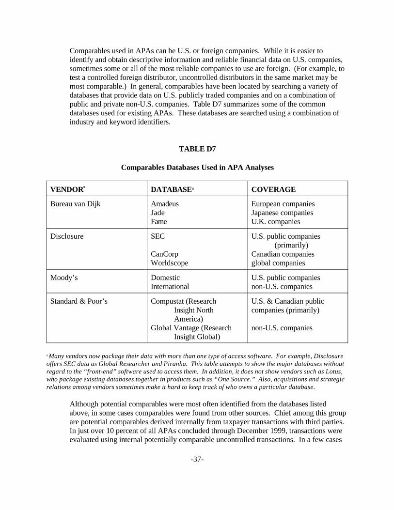
-37-

Comparables used in APAs can be U.S. or foreign companies. While it is easier toidentify and obtain descriptive information and reliable financial data on U.S. companies,sometimes some or all of the most reliable companies to use are foreign. (For example, totest a controlled foreign distributor, uncontrolled distributors in the same market may bemost comparable.) In general, comparables have been located by searching a variety ofdatabases that provide data on U.S. publicly traded companies and on a combination ofpublic and private non-U.S. companies. Table D7 summarizes some of the commondatabases used for existing APAs. These databases are searched using a combination ofindustry and keyword identifiers.

TABLE D7

Comparables Databases Used in APA Analyses

VENDOR* DATABASEa COVERAGE

Bureau van Dijk AmadeusJadeFame

European companiesJapanese companiesU.K. companies

Disclosure SEC

CanCorpWorldscope

U.S. public companies (primarily)

Canadian companiesglobal companies

Moody’s DomesticInternational

U.S. public companiesnon-U.S. companies

Standard & Poor’s Compustat (ResearchInsight NorthAmerica)

Global Vantage (ResearchInsight Global)

U.S. & Canadian publiccompanies (primarily)

non-U.S. companies

a Many vendors now package their data with more than one type of access software. For example, Disclosureoffers SEC data as Global Researcher and Piranha. This table attempts to show the major databases withoutregard to the “front-end” software used to access them. In addition, it does not show vendors such as Lotus,who package existing databases together in products such as “One Source.” Also, acquisitions and strategicrelations among vendors sometimes make it hard to keep track of who owns a particular database.

Although potential comparables were most often identified from the databases listedabove, in some cases comparables were found from other sources. Chief among this groupare potential comparables derived internally from taxpayer transactions with third parties. In just over 10 percent of all APAs concluded through December 1999, transactions wereevaluated using internal potentially comparable uncontrolled transactions. In a few cases

33Selection criteria are sometimes less specific for non-U.S. companies because there isnormally less publicly available descriptive information.

34Companies sometimes have financial data broken down by business line or geographicunits. Sometimes omitting one or more business or geographic segments can make a companymore comparable to the tested party. Thus, through the use of segmented data, an otherwiseunacceptable potential comparable might become acceptable. While such segmented comparablesmight be used in some cases, segment data is sometimes unreliable; the reliability must beexamined on a case-by-case basis.

-38-

comparables were found based on trade publications in specific industries, proprietarydatabases maintained by the taxpayer’s representative, and the taxpayer’s information oncompetitors.

Taxpayer representatives often have substantial resources for identifying potentialcomparables. Also, the APA Program prefers when possible to work with reasonableapproaches proposed by the taxpayer rather than to start from scratch. For both of thesereasons, the APA Program often relies to a large extent on a taxpayer’s comparablesearches. However, even when working from a taxpayer’s search, the Service’s APATeam will conduct its own searches when appropriate.

Selecting Comparables

• Scrutinize Potential Comparables

The initial list of companies from database searches can yield a number ofcompanies whose business activities may not be remotely comparable to those ofthe entity being tested. Therefore, so called “comparables” based solely on SIC orkeyword searches are almost never used in APAs.

Rather, pools of initially identified companies are accepted or rejected ascomparables based on a combination of quantitative and qualitative screens,business descriptions, and other information found in a company’s Annual Reportto shareholders and filings with the U.S. Securities and Exchange Commission(“SEC”).33 (The application of multiple quantitative screens to select comparables,without also analyzing descriptive information about the companies, generally hasnot been acceptable APA practice.) Normally, functions, risks, economicconditions, and the property (product or intangible) and services associated withthe transaction must be comparable. Determining comparability can be difficult,and is often at the heart of the APA Team’s work.34

• Selecting a Set

35“The arm’s length range will be derived only from those uncontrolled comparables thathave, or through adjustments can be brought to, a similar level of comparability and reliability, anduncontrolled comparables that have a significantly lower level of comparability and reliabilitywill not be used in establishing the arm’s length range.” Reg. 1.482-1(e)(2)(iii).

36For such comparables, “it is likely that all material differences have been identified”between the uncontrolled comparable and the controlled transaction. Further, each identifieddifference has “a definite and reasonably ascertainable effect on price or profit, and an adjustmentis made to eliminate the effect of each such difference.” Reg. § 1.482-1(e)(2)(iii)(A).

-39-

For selecting a final set of comparables, the standard in the regulations is that oneshould select the most comparable and reliable potential comparables, and onlyinclude potential comparables that are not “significantly” less comparable andreliable than the best ones available.35 However, this standard is susceptible todifferent interpretations, and choosing a set of comparables is an art rather than ascience.

In this regard, we should distinguish two situations. The first is the rare case whensome comparables are of high enough quality so that the arm’s length range wouldinclude all of their results.36 In such cases one normally should use thosecomparables to the exclusion of others, which normally would be deemed“significantly” less comparable or reliable. In principle, even just one suchcomparable would make an acceptable set, although a taxpayer might prefer to havemore comparables so as to define a range of arm’s length results instead of a singlepoint.

The second, more normal situation is that no such high quality comparables exist. In such cases, where even the best comparables give one some uneasiness, therecan be “strength in numbers.” Thus, including some additional comparables thatseem to be somewhat less comparable or reliable than the best ones can yield alarger set of comparables that produces a more reliable final result. When aninitial set of quantitative and qualitative screening criteria yielded a small set ofcomparables, the APA Team would often consider ways to relax the criteria to geta somewhat larger set.

There is no magic number of comparables to include. As a rough guide, havingthirteen or more would cause no uneasiness, having eight would cause slightuneasiness, and having only four would cause more substantial uneasiness. Butthese are just rough guides. Many APAs have used a range based on eight or fewercomparables, and some have used a range based on four or fewer comparables. Sometimes no additional comparables can be found of even roughly the samecomparability and reliability as the best ones.

• Criteria Used

37The lack of data does not always indicate startup or shutdown. For example, a companycan be acquired, after which there will be no more data available.

-40-

The APA Program has applied a combination of criteria to determine comparabilityof economic conditions. Specifically, it frequently has combined a “same industry”criterion with criteria focusing on the level of market served, the maturity of thecompany (minimum or maximum number of years of operation), and/or the marketserved (minimum or maximum percentage of sales in a geographic area and/orpercentage of government sales.)

In addition, the APA Program has generally required the potential comparables tohave complete financial data available for a specified period of time. Sometimesthis has been three years, but it can be more or less, depending on the circumstancesof the controlled transaction and the availability of good comparables. There is atension here. On the one hand, good comparables are often scarce, and requiring apotential comparable to have complete financial data for several years caneliminate a company that would make a good comparable. On the other hand, datafrom a very few years might represent atypical years of a company subject tocyclical fluctuations in business conditions. Also, a comparable with dataavailable for only a short period of years might be in a startup or shutdown period(and thus perhaps not sufficiently comparable to the tested party, assuming that thetested party during the APA years is not undergoing startup or shutdownactivities).37 Further, allowing comparables that do not have complete data for thewhole analysis window presents the issue of how to weight that comparable’sresults compared to other comparables’ results (see the next section, on analysiswindows).

Many additional criteria and/or screens have been applied in many cases. One is asales level screen. The rationale is that very different sales levels or transactionsizes might involve fundamentally different economic conditions (e.g. differenteconomies of scale, different negotiating power with suppliers and customers).

Another criterion is product similarity. Transactions involving different types ofproducts can face different economic conditions. The importance of productcomparability depends on the transfer pricing method being used (Reg. §1.482–1(d)(3)(v)). In using methods that rely on the identification of comparableuncontrolled companies, the APA Program has generally required less productcomparability than when using methods that rely on comparable uncontrolledtransactions. Nonetheless, product comparability, as determined from publiclyavailable corporate information, has often been used as a selection criterion whenpossible for uncontrolled companies.

38Memorandum of January 9, 2001, from Robert Weissler to APA Program ProfessionalStaff re: “CPM Comparables’ Abnormal Profit Levels: Minutes of Meeting of September 21,2000”.

-41-

Yet another criterion is financial distress. Companies in financial distress oftenhave experienced unusual circumstances that would render them not comparable tothe entity being tested. Recent thinking in the APA Program is that an unfavorableauditor’s opinion or bankruptcy during a particular year normally would make acompany not comparable for that year with a tested party that is not in similardistress. However, operating losses should not eliminate a potential comparableunless some additional factors are present. See Exhibit B.38

An additional important class of selection criteria involves the development andownership of intangible property. When the tested party does not own significantmanufacturing intangibles or conduct significant research and development(“R&D”), several criteria have been used to eliminate potential comparables thathave significant manufacturing intangibles or conduct significant R&D. Theseselection criteria have included determining the importance of patents or screeningfor R&D expenditures as a percentage of sales or costs. Quantitative screensgenerally have been used together with publicly available descriptive informationon the comparables.

Selection criteria relating to asset comparability and operating expensecomparability have sometimes been used. A screen of property, plant, andequipment (“PP&E”) as a percentage of sales or assets, combined with a reading ofa company’s SEC filings, has been used to help ensure that distributors (generallywith lower PP&E) were not compared with manufacturers (generally with higherPP&E), regardless of their SIC classification. Similarly, a test involving the ratioof operating expenses to either sales or total costs has helped to determine whethera company undertakes a significant marketing and distribution function. (However,in some cases lower or higher ratios of operating expenses to sales may indicateincreasing or decreasing sales, respectively, rather than functional differences.) This test has most often been used when complete descriptive information about acompany’s functions was not available.

DECIDING ON THE ANALYSIS WINDOW AND RELATED MATTERS

As described in the next three sections, the comparables’ results are adjusted as needed;the adjusted results are used to determine an arm’s length range; and the taxpayer’s resultsare tested against the arm’s length range. Before all that can happen, however, one must

39Multiple-year results of a controlled recipient of intangible property are also consideredunder the periodic adjustment provisions of Reg. § 1.482-4(f)(2). That section is concerned withthe statutory requirement under IRC § 482 that the compensation for an intangible be commensuratewith the income attributable to the intangible. Lesson 2 will address intangibles.

-42-

decide the time period over which to compute the comparables’ results, and certain relatedtechnical details.

In an audit context, for which the regulations were written, this choice of time period tendsto be fairly straightforward. Ordinarily, the comparable results “occurring in the taxableyear under review” will be used to test the tested party’s results for that year. (By the timea particular year is audited, comparables’ data for that year are almost always available.) However, certain circumstances warrant consideration also of data from the comparablesor the tested party “for one or more years before or after the year under review.” Normally, the same period is used for both the comparable data and the tested party data. Circumstances warranting the use of multiple year data include business cycles, product orintangible life cycles, and data availability issues. Reg. 1.482-1(f)(2)(iii) . When a CPMis used, “data from one or more years before or after the taxable year under review mustordinarily be considered.” However, “multiple-year data ordinarily will not beconsidered” when using the CUP method.39

The APA context is more complex, and is not directly addressed in the regulations. Thereason is that, because APAs are prospective, there is usually a mismatch between theperiod for which the comparables’ data is used (the “analysis window”) and the periodduring which the tested party’s results are evaluated (the “APA period” or “APA years”). For example, suppose that a calendar year taxpayer applies for an APA covering 2000-2004 on the last possible date, approximately September 15, 2001. The comparables’analysis in the taxpayer’s application probably would not include comparable data goingbeyond the year 2000. The taxpayer might propose an analysis based on comparable datafor 1998-2000.

In principle, it is possible to reduce this mismatch by updating the comparables’ results asthe APA period progresses. For administrative simplicity, there might be only one update. Thus, in the example just discussed, the arm’s length range applicable to years 2003 and2004 might be recomputed in 2003 based on the comparables’ results for 2000-2002. While this approach has occasionally been used, it is fraught with problems. How can onebe sure that the companies selected remain comparable to the tested party? Some might,for example, make major changes to their business. The Service and the taxpayer mightdisagree about particular companies. What if some or all of the original comparable set donot have data available for the new analysis period because they merged or went out ofbusiness? Then one might need to perform a new comparables search.

The APA Program typically has tried to use as late an analysis window as possible, toreduce the mismatch between the analysis window and the APA period. Sometimes, for

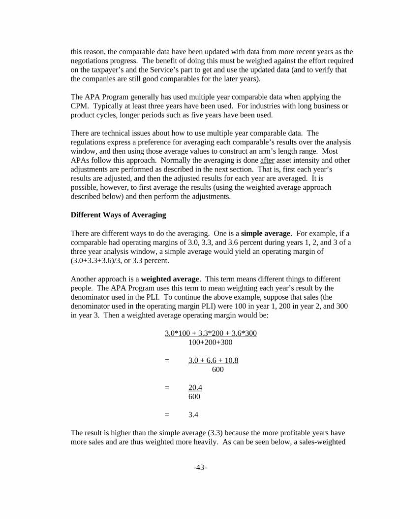
-43-

this reason, the comparable data have been updated with data from more recent years as thenegotiations progress. The benefit of doing this must be weighed against the effort requiredon the taxpayer’s and the Service’s part to get and use the updated data (and to verify thatthe companies are still good comparables for the later years).

The APA Program generally has used multiple year comparable data when applying theCPM. Typically at least three years have been used. For industries with long business orproduct cycles, longer periods such as five years have been used.

There are technical issues about how to use multiple year comparable data. Theregulations express a preference for averaging each comparable’s results over the analysiswindow, and then using those average values to construct an arm’s length range. MostAPAs follow this approach. Normally the averaging is done after asset intensity and otheradjustments are performed as described in the next section. That is, first each year’sresults are adjusted, and then the adjusted results for each year are averaged. It ispossible, however, to first average the results (using the weighted average approachdescribed below) and then perform the adjustments.

Different Ways of Averaging

There are different ways to do the averaging. One is a simple average. For example, if acomparable had operating margins of 3.0, 3.3, and 3.6 percent during years 1, 2, and 3 of athree year analysis window, a simple average would yield an operating margin of(3.0+3.3+3.6)/3, or 3.3 percent.

Another approach is a weighted average. This term means different things to differentpeople. The APA Program uses this term to mean weighting each year’s result by thedenominator used in the PLI. To continue the above example, suppose that sales (thedenominator used in the operating margin PLI) were 100 in year 1, 200 in year 2, and 300in year 3. Then a weighted average operating margin would be:

3.0*100 + 3.3*200 + 3.6*300100+200+300

= 3.0 + 6.6 + 10.8600

= 20.4600

= 3.4

The result is higher than the simple average (3.3) because the more profitable years havemore sales and are thus weighted more heavily. As can be seen below, a sales-weighted

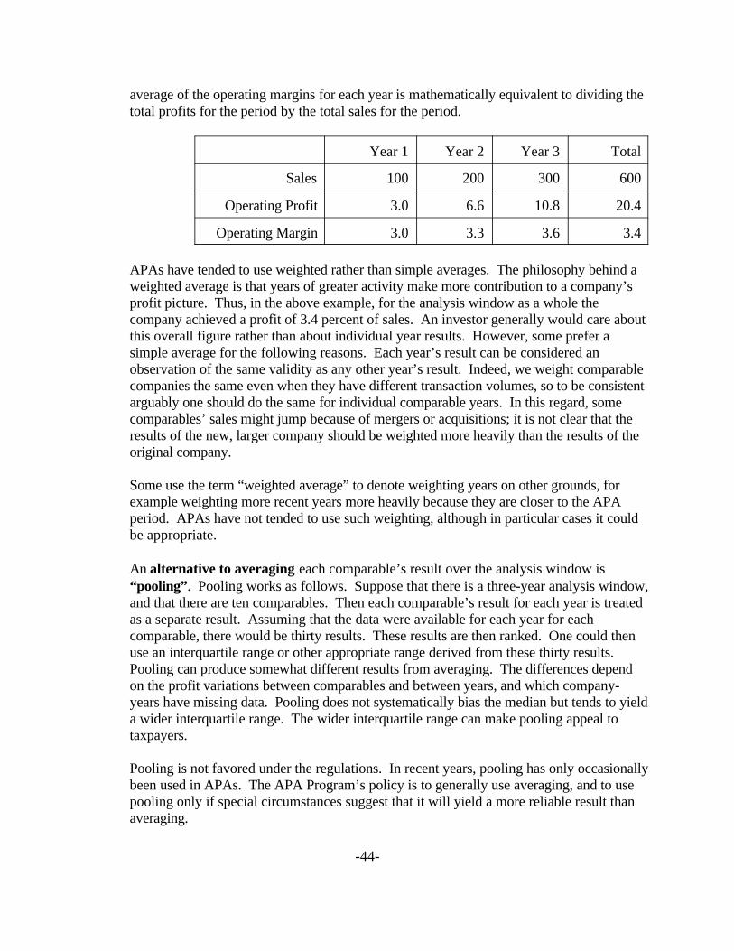
-44-

average of the operating margins for each year is mathematically equivalent to dividing thetotal profits for the period by the total sales for the period.

Year 1 Year 2 Year 3 Total

Sales 100 200 300 600

Operating Profit 3.0 6.6 10.8 20.4

Operating Margin 3.0 3.3 3.6 3.4

APAs have tended to use weighted rather than simple averages. The philosophy behind aweighted average is that years of greater activity make more contribution to a company’sprofit picture. Thus, in the above example, for the analysis window as a whole thecompany achieved a profit of 3.4 percent of sales. An investor generally would care aboutthis overall figure rather than about individual year results. However, some prefer asimple average for the following reasons. Each year’s result can be considered anobservation of the same validity as any other year’s result. Indeed, we weight comparablecompanies the same even when they have different transaction volumes, so to be consistentarguably one should do the same for individual comparable years. In this regard, somecomparables’ sales might jump because of mergers or acquisitions; it is not clear that theresults of the new, larger company should be weighted more heavily than the results of theoriginal company.

Some use the term “weighted average” to denote weighting years on other grounds, forexample weighting more recent years more heavily because they are closer to the APAperiod. APAs have not tended to use such weighting, although in particular cases it couldbe appropriate.

An alternative to averaging each comparable’s result over the analysis window is“pooling”. Pooling works as follows. Suppose that there is a three-year analysis window,and that there are ten comparables. Then each comparable’s result for each year is treatedas a separate result. Assuming that the data were available for each year for eachcomparable, there would be thirty results. These results are then ranked. One could thenuse an interquartile range or other appropriate range derived from these thirty results. Pooling can produce somewhat different results from averaging. The differences dependon the profit variations between comparables and between years, and which company-years have missing data. Pooling does not systematically bias the median but tends to yielda wider interquartile range. The wider interquartile range can make pooling appeal totaxpayers.

Pooling is not favored under the regulations. In recent years, pooling has only occasionallybeen used in APAs. The APA Program’s policy is to generally use averaging, and to usepooling only if special circumstances suggest that it will yield a more reliable result thanaveraging.

40Since these issues are raised by including comparables that lack data for the wholeanalysis window, one might consider excluding those comparables in the first place on the groundthat the less than complete data makes them unreliable. However, there may be a shortage of goodcomparables, and certain comparables with some data missing may otherwise appear quite good. The selection of comparables is discussed in the previous section.

-45-

Pooling might be considered in cases in which some of the comparables are missing datafor some years in the analysis window. Suppose there is a five-year analysis window, andthe selected comparables have data available for three, four, or five of those years. Ifaveraging were used, one comparable’s results based on only three years of data would beweighted the same as another comparable’s results based on five years of data. One mightargue, however, that the results based on three years of data should be given less weight. One way to weight less the comparables with only three years of data is by pooling, sinceeach comparable then contributes as many observations as it has years of data available.40

Even in cases of missing data, however, the APA Program will consider pooling onlywhen the taxpayer can make a specific showing that the comparables with less years ofdata should be weighted less. For example, a taxpayer might show that the comparablesare subject to strong cyclical variations, so that results based on fewer years are lessreliable. On the other hand, if the major profit variations are between companies, witheach comparable’s profit level fairly stable over the analysis window, then there would beno need to weight less the comparables with fewer years of data.

Sometimes taxpayers make the following argument for pooling. One cannot expect a testedparty’s annual results to meet an arm’s length range derived from comparables’ averageresults over multiple years, since those average results reflect a smoothing out of year-to-year variations. Thus, if the tested party’s results are tested on an annual basis, then thearm’s length range should be derived from comparables’ annual results (e.g., pooling)rather than comparables’ average results over multiple years. If a taxpayer makes such anargument, the APA Program normally would consider testing the tested party’s results overa multiple year period rather than using pooling.

ADJUSTING THE COMPARABLES’ RESULTS BECAUSE OFDIFFERENCES WITH THE TESTED PARTY

After the comparables have been selected, the regulations require that “[i]f there arematerial differences between the controlled and uncontrolled transactions, adjustmentsmust be made if the effect of such differences on prices or profits can be ascertained withsufficient accuracy to improve the reliability of the results.” Reg. § 1.482–1(d)(2).

Asset Intensity Adjustments

41For a more complete discussion, Brian Becker, “Capital Adjustments: A ShortOverview,” Transfer Pricing (BNA), Jan. 29, 1997, pp. 613-619.

-46-

One type of adjustment has been variously called an “asset intensity,” “balance sheet,” or“working capital” adjustment. This adjustment is performed when a CPM is used, eitherby itself or as part of another method such as a residual profit split.

• Reason for the Adjustments

Two concepts underlie the need for asset intensity adjustments. the first is that theamount of capital actively employed in a business normally affects a company’seconomic profit and expected return. The second is that hidden interest included ina company’s expenses or revenues should be removed. These concepts areexplained below.

The PLIs used with the CPM exclude explicit interest paid and received. Thereason is that the one is comparing profitability of operations. For example,consider three companies identical in all respects (e.g., working capitalrequirements, functions performed, sales, products, market, levels of accountspayable) except for capital structure. The first is completely financed by equity thatprovides for all working capital needs, with enough left over to purchase acertificate of deposit that pays interest equal to one percent of sales. The second iscompletely financed by equity that provides for all working capital needs, withnothing left over. The third meets its working capital needs partly by equity andpartly by taking out a long term loan on which it pays interest amounting to onepercent of sales. These companies’ before-interest profits will be the same, whiletheir after-interest profits will be different. For transfer pricing purposes, thesecompanies should be earning the same profit from operations, independent of theircapital structure. Therefore, the PLIs used to compare companies are defined toreflect profits before interest.

However, while the amount of money sitting in a long term deposit or owed on along term loan does not affect the profit earned from operations, the amount ofcapital actively employed in the business does. Actively employed capital canincrease operating profits in various ways. It can let a company:41

• offer credit to customers, who will then pay imputed interest in the purchaseprice, which will increase the reported operating profit.

• pay suppliers more promptly, resulting in lower prices, which will increasethe reported operating profit.

• hold more inventory, which can mean buying in bigger quantities fromsuppliers and/or offering quicker response to customers’ needs. Both of

42According to economic theory, a rational company would carry capital only to the extentthat the increased profits at least paid the carrying cost. Under the law of diminishing returns, asthe capital carried increases, each additional unit of capital increases profits less than the previousunit. A rational company will keep employing additional capital until, at the margin, the returnfrom the next unit of capital equals the cost to carry the capital.

43Robert Weissler, memorandum to Study Group on Consistency in Asset IntensityAdjustments, re: “Partial Survey of Issues,” Sept. 18, 2000.

-47-

these actions will increase reported operating profit, since the suppliersinvolved will offer discounts and the customers involved will pay apremium.

• own facilities and equipment that can increase operating profit.

Asset intensity adjustments are designed to adjust nominal profit levels to reflectthat companies with higher levels of actively employed capital are expected tohave higher profit levels. Typically, when one makes asset intensity adjustments,one assumes that the extra capital in question increases operating profit by anamount equal to the company’s cost to carry the extra capital.42 The carrying costhas often been defined as a borrowing rate such as the prime rate, but sometimes ahigher rate such as the taxpayer’s weighted average cost of capital would be moreaccurate.

The asset levels are compared on a relative basis. For example, for PLIs whosedenominator is sales (e.g., operating margin), the APA Program comparescompanies on the basis of assets per sales. The logic behind this approach is asfollows. If each dollar of capital employed increases a company’s operating profitby an amount y, then D dollars of capital employed increases the operating profit byDy, and increases the operating margin (which is operating profit divided by sales)by Dy/S. So it is the ratio of D to S (i.e., assets per sales) that determines the effectof the capital employed on the operating margin. This concept is behind the name“asset intensity”: one does not compare companies’ absolute asset level, but rathercompares their asset ratios or intensities (in this example, the ratio of assets tosales).

In some cases the benefit provided by an asset might be much different from itscarrying cost, so that the normal type of adjustment would not be appropriate. Forexample, a sudden market downturn could result in the buildup of largeunproductive inventories; and customers in distress might take a long time to paybut fail to pay the proper imputed interest. For a discussion of this issue andothers, see Exhibit C.43

• Types of Assets Adjusted For

-48-

The types of assets adjusted for depend on whether the PLI has an income statementitem in the denominator (e.g., operating margin, Berry ratio, markup on total costs)or a balance sheet item in the denominator (ROA, ROIC).

• PLIs with an Income Statement Item in the Denominator

The most common assets adjusted for in APAs include accounts receivable,inventory, and accounts payable (a negative asset, a type of non-interest-bearing liability), corresponding to the first three bullets above. Inpractice, when data has been available, most APAs have included theseadjustments, regardless of whether or not their effect is material.

Another asset adjusted for in APAs is plant, property, and equipment(PP&E), corresponding to the fourth bullet above. While this adjustmenthas been omitted in many APAs, the current thinking in the APA Program isthat in most cases this adjustment is appropriate because additional PP&Enormally enables a company to make additional profit. Sometimes thePP&E adjustment is done using a medium term interest rate while short terminterest rates are used for accounts receivable, inventory, and accountspayable. This difference reflects that PP&E is a longer-term asset than theothers.

Other assets have rarely been adjusted for. However, the current thinking inthe APA Program is that in principle, virtually all productive assetsactively employed in the business (including negative assets in the form ofnon-interest-bearing liabilities) should be adjusted for. This wouldinclude, for example, cash necessary for working capital purposes, prepaidexpenses, and accrued expenses (a non-interest-bearing liability).

Two limitations should be noted. First, interest-bearing assets or liabilitieswould not be included. Interest-bearing assets normally represent eitherpassive investments, which are not actively employed in the business, oritems like receivables with an explicit interest charge. When receivableshave an explicit interest charge, the sales price and operating profit areunaffected by the credit extended, since the extra income is recorded asinterest income rather than as in increase to the sales price. Similarly,interest-bearing liabilities result in explicit interest payments rather than,for example, an increased price of goods from suppliers. Second,intangible assets typically should not be adjusted for because one typicallycannot value intangibles across companies on a consistent basis (see theearlier discussion of the CPM using a return on assets PLI).

• PLIs with a Balance Sheet Item in the Denominator

44If the interest rate used for calculating the NIBLs adjustment were the same as thecompany’s overall return on assets, then the ROA and ROIC PLIs would yield the same result.

-49-

When a return on assets (ROA) PLI is used, an adjustment is normallyneeded to account for differences in non-interest-bearing liabilities (NIBLs)such as accounts payable. Indeed, a company with more accounts payablewill pay more imputed interest as part of its purchase price, which willdepress operating profit. This adjustment makes the ROA result closer tothe result one would get using a return on invested capital (ROIC) PLI. Typically, the adjustment is made using a debt rate of return, which isnormally lower than the weighted average cost of capital that applies to acompany as a whole.44

Given that the NIBLs adjustment is often performed using a lower rate ofreturn, one could then argue that if accounts payable receive a special lowerrate of return then so should accounts receivable, which are similar innature. If so, an adjustment should be made to reflect a lower return foraccounts receivable. (Regulation 1.482-5(e), Example 5, gives an exampleof an accounts receivable adjustment when using ROA.) One might alsoargue that in some cases other assets should receive special rates of return,as reflected by an appropriate adjustment. For example, arguably in somecases inventory should earn a different rate of return than plant, property,and equipment.

There is less need for asset intensity adjustments when a return on investedcapital (ROIC) PLI is used. This PLI already accounts for differences inNIBLs such as accounts payables, since NIBLs are subtracted from the assetbase. More generally, the philosophy behind a return on invested capitalPLI is that different asset types are fungible, and that regardless of assetmix, the investors in a company need a certain return on their investment. Following this philosophy, one would not assign different rates of return todifferent asset types. However, in particular cases one still might argue fordifferent rates of return.

• Computing the Adjustments

Conceptually, one can perform adjustments in one of three ways:

1) Adjust the comparables to the tested party. Adjust each comparable’s resultto be the result the comparable would have had if it had had the testedparty’s asset intensities. Derive an arm’s length range from thecomparables’ adjusted results, and test the tested party’s results against thatrange.

-50-

2) Adjust the tested party to the comparables. Derive an arm’s length rangefrom the comparables’ unadjusted results. Before comparing the testedparty’s results against that range, adjust the tested party’s results to be whatthey would have been if the tested party had the comparables’ assetintensities. (If there are more than one comparable, one might use averageasset intensity figures across the whole set of comparables.)

3) Adjust both the tested party and the comparables to asset intensities of zero. Adjust each comparable’s result to be the result the comparable would havehad if its pertinent asset intensities were zero. Derive an arm’s length rangefrom the comparables’ adjusted results. Before comparing the testedparty’s results against that range, adjust the tested party’s results to be whatthey would have been if the tested party’s pertinent asset intensities were zero.

In principle, all three approaches should yield the same results, except that thesecond approach could yield somewhat different results because one is notseparately using each comparable’s asset intensities. The first and thirdapproaches are most commonly used. The APA Program typically has used thefirst approach.

The precise formulas used to perform these adjustments have been the subject ofmuch discussion. Many versions used, differing in various technical details. Unfortunately, there is no good reference discussing the variations and their prosand cons. Fortunately, the different formulas tend to achieve similar results.

The APA Program has generally required that tested party’s and comparables’ databe compared on a first-in first-out (“FIFO”) inventory accounting basis. Althoughfinancial statements may be prepared on a last-in first-out (“LIFO”) basis, crosscompany comparisons are less meaningful when one or more companies use LIFOinventory accounting methods. Thus, if the tested party and/or comparables havedata stated on a LIFO basis, the data must first be converted to a FIFO basis beforeany asset intensity adjustments are done. This conversion is straightforward; itmakes used of the “LIFO Reserve” accounting item. This conversion directlyaffects costs of goods sold and inventories. Since it affects cost of good sold, ittherefore affects profitability, even before asset intensity adjustments areperformed.

To compare the profits of two entities with different relative levels of receivables,inventory, payables, and (in some cases) PP&E, the APA Program has estimatedthe carrying costs of each item and adjusted profits accordingly. Althoughsomewhat different formulas have been used in specific APA cases, Exhibit Dpresents one set of formulas used in many APAs. These formulas are used in the

45TPTOOL consists of a report file and a concepts file, with documentation, that run onCompustat’s Research Insight user interface. TPTOOL accesses Compustat’s North Americandatabase for information on comparables. The user inputs the tested party’s asset intensities andinputs appropriate carrying costs. The software then performs asset intensity adjustments(adjusting the comparables to the tested party) and computes interquartile ranges. The softwarewas initially developed in 1997 and 1998 by Robert Weissler of the APA Program, and has beenmodified some since then. The current documentation consists of the original documentation datedMarch 5, 1998, and a package of emails and memos describing subsequent changes.

46The regulations do not directly address how to compute a yearly average asset level inthe context of asset intensity adjustments. However, in defining operating assets for the purpose ofa return on assets PLI, the regulations mandate using the average of the beginning and end of yearasset levels “unless substantial fluctuations . . . make this an inaccurate measure of the averagevalue over the year,” in which case a more accurate measure of that average value must be used. Reg. § 1.482-5(d)(6).

-51-

APA Program’s “TPTOOL” software,45 but they do not represent any officialposition of the APA Program or the Service.

The software estimates comparables’ year-average asset levels by averaging thebeginning and end of year levels. This is fairly standard practice in the Service andwith practitioners. However, it can lead to inaccuracies. For example, if adistributor has a somewhat seasonal business with inventories elevated in thesummer, and has a December fiscal year end, then averaging the levels from twoconsecutive year ends would underestimate the average inventory during theintervening year. In such a case, one might consider averaging comparables’quarterly data.46

The tested party’s year-average asset levels are also by common practice computedby averaging the beginning and end of year levels. However, in particular cases adifferent approach should be used. As with comparables, there may be an issue ofseasonal fluctuations. The tested party may have other unusual fluctuations ortrends in asset levels that make the normal approach inaccurate. A practicalalternative approach is sometimes to take the average of monthly levels.

Another issue sometimes arises concerning the tested party’s asset levels. Conceptually, the comparables’ results and the comparables’ and tested party’sasset intensities in the analysis window are used as a proxy for what these resultsand asset intensities are expected to be during the (usually later) APA years. Typically the assumption that the APA years will be similar to the analysis windowin this regard seems reasonable, so that one proceeds on that basis. However, insome cases this assumption is not accurate. In one executed APA, the tested party’sreceivables intensity climbed substantially between the analysis window and theAPA years. Had the asset intensity adjustments been recomputed using actual

-52-

balance sheet amounts, the computed arm’s length range of operating marginswould have changed significantly in the direction of increased profitability. Whenthat APA came up for renewal, the APA Team and the taxpayer agreed to performthe asset intensity adjustments for receivables differently for each APA year,depending on the tested party’s receivables level in that year. In the renewalnegotiations, the Service also argued that certain other tested party asset intensitiesduring the analysis window were aberrational and therefore not a good proxy forexpected intensities during the APA period. The Service and the taxpayer agreedto substitute other values for some historical asset intensities, based on theintensities in other, more normal years of the analysis window.

• Regulatory Provisions

The regulations recognize the need for asset intensity adjustments but do notextensively discuss them. In general, reg. 1.482-1(d)(2) provides that if “there arematerial differences between the controlled and uncontrolled transactions,” then“adjustments must be made if the effect of such differences on prices or profits canbe ascertained with sufficient accuracy to improve the reliability of the results.”

In discussing the CPM, the regulations under 1.482-5 build on this generalprinciple. Reg. 1.482-5(c)(2)(iv) provides:

Adjustments for the differences between the tested party and theuncontrolled taxpayers. If there are differences between the tested partyand an uncontrolled comparable that would materially affect the profitsdetermined under the relevant profit level indicator, adjustments should bemade according to the comparability provisions of Sec. 1.482-1(d)(2). Insome cases, the assets of an uncontrolled comparable may need to beadjusted to achieve greater comparability between the tested party and theuncontrolled comparable. In such cases, the uncontrolled comparable'soperating income attributable to those assets must also be adjusted beforecomputing a profit level indicator in order to reflect the income and expenseattributable to the adjusted assets. In certain cases it may also beappropriate to adjust the operating profit of the tested party and comparableparties. For example, where there are material differences in accountspayable among the comparable parties and the tested party, it will generallybe appropriate to adjust the operating profit of each party by increasing it toreflect an imputed interest charge on each party's accounts payable.

This provision thus recognizes asset level differences as a reason for adjustmentsand specifically mentions differences in accounts payable. It also recognizes that

47The preamble also states that “differences in non-interest-bearing liabilities (such asaccounts payable) that would materially affect operating profit generally should be reflected byadjustments to operating profit to reflect an imputed interest charge on each party’s liability.” Thepreamble thus recognizes non-interest bearing liabilities as a larger class of assets subject toadjustment, of which accounts payable is one example.

48It is not clear why this example compares levels of receivables relative to sales. Whenusing a return on capital employed PLI, most economists would compare levels of receivablesrelative to capital employed. The drafters of this example likely missed this point.

-53-

one might as a matter of implementation perform adjustments just to thecomparables or to the comparables and the tested party.47

Two examples in regulation 1.482-5(e) also discuss asset intensity adjustments. Example 5 involves a return on capital employed PLI and an adjustment foraccounts receivable. The adjustment is stated as follows:

Each uncontrolled comparable’s operating assets is reduced by the amount(relative to sales48) by which they exceed [the tested party’s] accountsreceivable. Each uncontrolled comparable’s operating profit is adjusted bydeducting imputed interest income on the excess accounts receivable. Thisimputed interest income is calculated by multiplying the uncontrolledcomparable’s excess accounts receivable by an interest rate appropriate forshort-term debt.

Thus, this example specifically mentions accounts receivable and uses a short-termdebt rate to adjust that asset.

Example 6 does not specify the PLI used and assumes differences in accountspayable:

To adjust for these differences, the district director increases the operatingprofit of the uncontrolled distributors and [the tested party] to reflectinterest expense imputed to the accounts payable. The imputed interestexpense for each company is calculated by multiplying the company’saccounts payable by an interest rate appropriate for its short-term debt.

This example uses a short-term debt rate for accounts payable.

The regulations do not further discuss asset intensity adjustments. While theregulations touch on some of the issues, they do not provide a developedframework for analysis. Economic analysis must take over where the regulationsleave off.

49During the APA term, before the tested party’s results are tested for compliance with theagreed TPM, those results must be put on the same accounting basis as that used to adjust thecomparables (e.g., FIFO inventory accounting, same treatment of inventory writeoffs).

-54-

Other Adjustments

Aside from asset intensity adjustments, other types of adjustments are sometimesperformed. Sometimes the adjustments are done on an individual basis to each comparable(as asset intensity adjustments are done), and sometimes the adjustments are done to allcomparables in the same way. In the latter case, one is typically adjusting for a specialcircumstance of the tested party that distinguishes it equally (as far as the available dataindicates) from all of the comparables.

• Accounting Adjustments

Accounting adjustments are sometimes done to put all companies on a consistentbasis. These adjustments normally are done on an individual basis to eachcomparable. One adjustment normally done, already mentioned above inconnection with asset intensity adjustments, is to put all companies on a FIFO basisfor inventory accounting. Certain circumstances may warrant other accountingadjustments. For example, companies may differ in how they treat customer rebates(as a deduction from sales or an operating expense) or writeoffs from obsoleteinventory (as cost of goods sold, operating expense, or extraordinary expense). Generally, such adjustments are made only if an accounting issue seems importantand if it is possible to get sufficient data to perform the adjustment.49

• PLI Adjustments

The earlier discussion of the CPM method (in the section on TPMs) explained thatone can partly or fully transform one PLI into another by adding certain financialresults of the tested party to the comparables’ results. For example, one mightcompute an operating margin range for the comparables but then add in the testedparty’s operating expenses to get a gross margin range. Another way to think of thisapproach is that one starts with each comparable’s gross margin and then adjuststhat gross margin by adding the difference between the tested party’s operatingexpenses and the comparable’s operating expenses. Adding this differenceconstitutes an “operating expenses” adjustment, which is done individually for eachcomparable.

• Other Adjustments Used

Sometimes adjustments have been performed to account for differences in currencyrisk (to be discussed in Lesson 2) or functions such as R&D and manufacturing. Occasionally, there also have been adjustments for startup costs, geographic market

50 Sometimes taxpayers have proposed a geographic market adjustment that is in effect anadjustment for the different costs of capital to operate in those two markets. If a balance sheetbased PLI is used (e.g., return on assets, return on capital employed), then the comparable’sreturns could be adjusted based on the difference in cost of capital between the two markets. If anincome statement based PLI is used (e.g., operating margin, markup on total costs), then thecomparable’s returns could be adjusted using a variant of the normal asset intensity adjustments, inwhich the comparable and the tested party each have a different carrying cost for the assets inquestion. Such a modified asset intensity adjustment, if proposed by the taxpayer, would requirecareful scrutiny. One concern would be to make sure that the approach is sound in business andeconomic terms. Another concern is that certain approaches, if accepted in one case, might beimproperly extended by treaty partners or taxpayer representatives to other cases.

-55-

(see Reg. 1.482-1(d)(4)(ii)), cost of capital variations,50 nonroutine intangibles,sales shocks (i.e., dramatic unexpected changes in sales levels), and productliability. These adjustments have been evaluated on a case by case basis and madeonly when doing so improved the reliability of the results. They are sometimesdone individually for each comparable, and sometimes done the same way for allcomparables.

Sometimes an adjustment applies only to some of the APA years. For example, onecase involved a distributor whose business suffered during a particular yearbecause of a recession in its parent’s country. The Service and the taxpayerdiscussed possible adjustments to reflect that the distributor would not be expectedto earn a normal profit in that year.

As a matter of computation, when an adjustment applies only to some of the APAyears (or applies differently from one APA year to the next) and the tested party’sresults are tested on a multiple-year basis (as discussed in the section below ontesting and adjusting the tested party’s results), it is simpler to make an adjustmentto the tested party’s results before they are compared to the applicable range, ratherthan making an adjustment to the range for that particular year. For example,suppose that an APA specifies an operating margin of 2.0 percent to 4.0 percent,except that for one year the range would be adjusted downward by 1.0 percent. Inthat year, one could for computational purposes leave the range at 2.0 to 4.0 percentbut increase the tested party’s result by 1.0 percent before comparing it to therange. Then it is straightforward to average results from different years, since theyall are subject to the same range. If, for example, the taxpayer must in each APAyear meet the range on the basis of the average operating margin for that year andthe two previous years, then one can simply average the results for a three-yearperiod (including an increase of 1.0 percent for the special year) and compare theaverage to the range of 2.0 to 4.0 percent.

• Taxpayers’ Proposed Adjustments Supported by Regression Analysis

51Cf. Reg. 1.482-1(d)(3)(ii)(C), Example 2 (when discounts are given to variousuncontrolled customers depending on volumes, linear extrapolation is not reliable to determine thediscount for a controlled customer with volume much higher than all the uncontrolled customers).

-56-

Taxpayers sometimes propose creative adjustments supported by statisticalregression analysis. For example, if the tested party is a Japanese distributor ofscientific instruments, a taxpayer might present statistical evidence that in thisindustry in Japan the distributor’s profit level increases with the level of imports. The taxpayer would then propose adjusting each comparable’s profit level to whatit might have been if the comparable had had the same level of imports as the testedparty. Such arguments can be valid. In one bilateral case, the APA Programincluded in a recommended negotiating position such an adjustment based on theeffect of sales fluctuations on profits. However, these arguments from taxpayersrequire careful scrutiny as follows.

First, does the taxpayer’s analysis make economic sense? To continue the aboveexample, suppose the tested party sells only imports because its goods come fromits foreign parent, while the comparables all sell between 30 and 70 percentimports. Does the level of imports have the same economic meaning for both thecomparables and the tested party? For example, the comparables might tend toimport only certain specialty products that have higher margins. Thus, comparableswith more imports will have higher margins. However, the tested party may importa full line of instruments, mostly unspecialized, from its foreign parent. Then a highlevel of imports would not have the same significance. Also, it is in any eventquestionable that one can reliably extrapolate from comparables with 30 to 70percent imports to the case of 100 percent of imports.51 If import level isimportant, perhaps one should seek comparables closer in this regard to the testedparty. (One might still then do the suggested adjustment, but it would be morereliable.)

Second, is the taxpayer’s analysis statistically sound? Is the regression omittingother explanatory variables that should be added? Is the regression’s sample sizelarge enough? Several other questions could be asked.

Third, even if the taxpayer’s analysis makes economic sense and is statisticallysound, bear in mind that the taxpayer may have tried many possible adjustments andcarefully engineered one that gives a desired result. Does the taxpayer’s resultseem fair? Also, might the Service propose other adjustments that might seemequally justified but give opposite results?

CONSTRUCTING A RANGE OF ARM’S LENGTH RESULTS

52The term “transaction” here can include many transactions by one company, consideredon an aggregate basis. See Reg. § 1.482-1(f)(2)(iv) (product lines).

-57-

The types of ranges used in APAs completed through December 1999, are set forth inTable D8. The terms used in this table are defined below.

TABLE D8Types of Ranges

In APAs Concluded Through December 1999

Type of Range Number of APAsThat Involve ThisType

Full range 5

Interquartile range 41

Interquartile range recomputed after Tukey filter 5

Agreed range 11

Floor (result must be no less than x) 20

Ceiling (result must be no more than x) 4

Specific result 144

Financial products - statistical confidence interval to test for internal CUP 16

Arm’s Length Range

Reg. § 1.482–1(e)(1) states that sometimes a pricing method will yield “a single result thatis the most reliable measure of an arm’s length result.” Sometimes, however, a methodmay yield “a range of reliable results,” called the “arm’s length range.” A taxpayer whoseresults fall within the arm’s length range will not be subject to adjustment.

Under Reg. § 1.482–1(e)(2)(i), such a range is normally derived by considering a set oftwo or more uncontrolled transactions52 of similar comparability and reliability. If these

53For such comparables, “it is likely that all material differences have been identified”between the uncontrolled comparable and the controlled transaction. Further, each identifieddifference has “a definite and reasonably ascertainable effect on price or profit, and an adjustmentis made to eliminate the effect of each such difference.” Reg. § 1.482-1(e)(2)(iii)(A).

54One statistical method occasionally considered with large sets of comparables is toassume that the comparables’ results are a random sample of a larger set of results with a normaldistribution. One can then use statistical techniques to estimate that larger set’s median andstandard deviation based on the observed comparables’ results. By the definitions of normaldistribution and standard deviation, a range extending 0.675 standard deviations in either directionfrom the median will contain 50% of the members of the assumed larger set of results, with 25% ofthe members of that set lying above this range and 25% of the members lying below this range.

55“For purposes of this section, the interquartile range is the range from the 25th to the 75thpercentile of the results derived from the uncontrolled comparables. For this purpose, the 25thpercentile is the lowest result derived from an uncontrolled comparable such that at least 25percent of the results are at or below the value of that result. However, if exactly 25 percent of theresults are at or below a result, then the 25th percentile is equal to the average of that result and thenext higher result derived form the uncontrolled comparables. The 75th percentile is determinedanalogously.” Reg. § 1.482–1(e)(2)(iii)(C).

-58-

comparables are of very high quality, as defined in the Regulations,53 then under Reg.§1.482–1(e)(2)(iii)(A) the arm’s length range includes the results of all of the comparables(from the least to the greatest). However, the APA Program has only rarely identifiedcases meeting the requirements for the full range. If the comparables are of lesserreliability, then under Reg. § 1.482–1(e)(2)(iii)(B) “the reliability of the analysis must beincreased, where it is possible to do so, by adjusting the range through application of avalid statistical method to the results of all of the uncontrolled comparables.” Thereliability “is increased when statistical methods are used to establish a range of results inwhich the limits of the range will be determined such that there is a 75 percent probabilityof a result falling above the lower end of the range and a 75 percent probability of a resultfalling below the upper end of the range.” One such method, the “interquartile range,”“ordinarily provides an acceptable measure of this range,” although a different statisticalmethod “may be applied if it provides a more reliable measure.”54 In the case of bilateralAPAs, other methods for setting a range have been agreed upon between the CompetentAuthorities.

Interquartile Range

The “interquartile range” is the range from the 25th to the 75th percentile of thecomparables’ results. The precise definition in the regulations55 is somewhat difficult tounderstand. Table D9 shows how to compute the interquartile range for comparable sets of

56The table starts with a set of only one comparable and literally follows the definition inthe regulations. However, for sets of one to three comparables, one might question howmeaningful the definition of the interquartile range is. In those cases, the interquartile range isdefined to be the same as the full range.

-59-

different sizes. The table shows a recurring pattern that can be extended indefinitely.56 Inthe table’s center and right columns, 1 denotes the lowest comparable result, 2 denotes thenext lowest comparable result, and so on.

-60-

Table D9

Interquartile Ranges

Number of Comparables Bottom of Interquartile Range Top of Interquartile Range

1 1 1

2 1 2

3 1 3

4 average of 1 and 2 average of 3 and 4

5 2 4

6 2 5

7 2 6


9 3 7

10 3 8

11 3 9


13 4 10

14 4 11

15 4 12


17 5 13

18 5 14

19 5 15

A variant on the interquartile range involves a “Tukey filter,” as follows. First, the set ofcomparables is used to derive a standard interquartile range. Then the difference Dbetween the top and bottom of the interquartile range is computed. Next, all comparableswhose results are more than a certain multiple of D (often the multiple 1.5 is used) outsidethe interquartile range are discarded as “outliers.” Finally, the reduced set of comparables(without the outliers) is used to compute a second interquartile range, which is then used asthe arm’s length range. This approach has only occasionally been used for APAs (see

57The use of only one comparable transaction is more likely when that transaction is an“internal” comparable uncontrolled transaction, that is, a transaction that involves one of therelated parties under evaluation.

-61-

Table D8). The Tukey filter has been used to eliminate companies that were so anomalousthat they arguably should not have been included as comparables in the first place. Taxpayers have argued that proper comparable selection plus use of the interquartile rangeshould eliminate anomalous companies, and that adding a Tukey filter is a redundantsafeguard that unduly narrows the arm’s length range.

Specific Result (“Point”)

Even though a set of comparables could yield a range of results, some APAs havespecified a single or specific result, also called a “point.” This approach has been used insome APAs to avoid the possibility of manipulation to produce a result near the bottom ofa specified range. For bilateral APAs, each country might be concerned about the potentialfor such manipulation, making it easier for the two countries to agree on a specific resultthan on a range. In many APAs, the specific point has been the median point of the set ofcomparables’ results. However, in some APA cases, arguments for a different point havebeen made and accepted.

APAs also have often used a point in establishing a royalty rate. A set of comparables mayyield a range of possible arm’s length royalty rates. However, as a matter of businesspractice, companies typically fix precise royalty rates in advance. Therefore, APAs oftenrequire a specific royalty rate. Other methods in which a point rather than a range has beenused include CUP, resale price, and cost plus. Sometimes only one comparable transactionis used,57 yielding a specific result rather than a range. A point has also been used withCPM and with profits splits (discussed later). A point has commonly been used whenapplying the CPM to determine an arm’s length markup for integral services.

Floors and Ceilings

Some APAs specify not a point or a range, but a “floor” or a “ceiling.” When a floor isused, the tested party’s result must be greater than or equal to some particular value. Whena ceiling is used, the tested party’s result must be less than or equal to some particularvalue. Such an approach has been used, for example, where the TPM is a CPM withoperating margin as the PLI and the comparable transactions reflect certain currentbusiness conditions that might improve. The APA required that the tested party’s operatingmargin should always be above the bottom of the interquartile range, but permitted theoperating margin to go above the top of the interquartile range in case conditions improved.

Floors and ceilings are normally used only in unilateral APAs, to guarantee at least acertain minimum level of U.S. income or maximum level of foreign income. For bilateralAPAs, the treaty partner normally would object to an approach that put a minimum but no

-62-

maximum on U.S. income. Current APA Program practice does not favor the use of floorsor ceilings.

Approaches for Profit Splits

APAs have tended to adopt a point rather than a range when applying profit split methods. In some cases the choice of point or range, or the size of the range, has been an importantnegotiating point.

• Comparable Profit Split

In a comparable profit split under Reg. §1.482–6(c)(2), total profit is split in thesame ratio as the profit of comparable uncontrolled parties is split. Typically thismethod produces a specific ratio of profit split, although if more than one set ofcomparable parties were used it would be possible to derive a range. (Only oneAPA has ever used a comparable profit split.)

• Residual Profit Split

In a residual profit split under Reg.§ 1.482–6(c)(3), each party is first assigned aroutine return, and any residual profit or loss is split according to each party’srelative contribution of pertinent intangible property. Normally, the proportion inwhich to split the residual is a specific result that comes from specific valuesassigned to each party’s intangible contribution.

As normally implemented, this method also uses a specific result for the routinereturns. This approach is the simplest. Then for each APA year, the total U.S.profit, which consists of the U.S. routine return and the U.S. share of the residualprofit or loss, will be a specific result. However, in some APA negotiations, thetaxpayer has argued that the regulations entitle it to the interquartile range of eachroutine return. Under this approach, any total U.S. profit that results from anycombination of routine returns within these ranges (and from splitting the residualprofit or loss as agreed) is deemed to be arm’s length.

The regulations do not give clear guidance on whether taxpayers are entitled tosuch interquartile ranges. Reg. 1.482-1(e) explains that a taxpayer is permitted anarm’s length range, defined by the comparables, which can be either the full range,the interquartile range, or some other suitable range. However, this section of theregulations does not appear to contemplate a TPM in which two sets of rangeswould be used to generate a final result. Reg. 1.482-6(c)(3)(iii) gives an exampleof a residual profit split in which a point value is used for the routine profit.

• “Profit Creation”

58The treaty partner has also used the term “loss creation” for the situation in which oneparty has a loss despite an overall system profit. The treaty partner has similar concerns about“loss creation.” With both “profit creation” and “loss creation,” one party has a profit and theother a loss.

-63-

Another issue bearing on the range used in a residual profit split is what one treatypartner has called “profit creation”. This term term refers to the situation in whichone party to a controlled transaction earns a profit even though there is a totalsystem loss from the transactions at issue.58 This can occur when there is a residualloss after routine profits are taken. For example, suppose the tested partymanufacturer’s expected routine profit is $4M and the tested party distributor’sexpected routine profit is $8M, but there is a system loss of $2M. There is then aresidual loss of $14M. Suppose that this loss is split 50/50 ($7M each). Then themanufacturer’s total profit will be $4M minus $7M, or -$3M, while thedistributor’s total profit will be $8M minus $7M, or $1M. The distributor thusmakes $1M profit despite a system loss of $3M.

The Service’s position is normally that if the TPM was properly chosen, such“profit creation” is correct. However, one treaty partner finds such “profitcreation” troubling. To accommodate this concern, the Service in some cases hasagreed on constraints that minimized the extent of “profit creation.” For example,in some cases involving a profit split range, a constraint was added that eachparty’s profit could not exceed the greater of (1) zero, (2) the system profit, and (3)the bottom of the range as originally determined. Thus, a party could not earnabove the bottom of its range if that would give the party positive profit greater thanthe system profit.

• Other Profit Splits

The various points just discussed concerning ranges under a residual profit splitcould also apply to an unspecified profit split structured similarly to residual profitsplits. Such a TPM would assign a routine profit to each party and then split theresidual in some manner other than according to intangible contributions as wouldbe required for a residual profit split under Reg. 1.482-6(c)(3).

Statistical Confidence Intervals

Some APAs involving financial products have employed a “statistical confidence interval”to compare pricing of a large set of controlled transactions with a comparable set ofuncontrolled transactions. An example is a financial institution with fairly autonomousbranches in several countries. Pursuant to the business profits article of the applicableincome tax treaties and Prop. Reg. §1.482–8(b), APAs have been executed allowing thetaxpayer to allocate profits between branches with reference to the branches’ internal

59Averages can be computed on a simple basis (averaging the numerical results from eachyear) or on a weighted average basis, which is equivalent to taking total results for the wholeperiod (e.g., total operating profit divided by total sales, to yield a total or a weighted averageoperating margin). These concepts are discussed above in the section on analysis windows. Theweighted average approach is often considered preferable since it reflects the taxpayer’s totalresults.

Averaging can be mathematically tricky if the range is not the same for each APA year. Asolution to this problem is to keep the range the same each year and make a special adjustment tothe tested party’s results in particular years before comparison with the range. This approach isdescribed earlier in the section on adjusting the comparables’ results.

60In an audit context, if “data relating to uncontrolled comparables from multiple years isused, data relating to the controlled taxpayer for the same years ordinarily must be considered.” Reg. 1.482-1(f)(2)(iii)(A). However, as discussed above in the section on analysis windows, in

-64-

accounting methods, taking into account all trades, including interbranch and/or interdesktrades. In order for this method to provide a reliable result, however, it is necessary toensure that all such controlled trades be priced on the same market basis as uncontrolledtrades. To test whether this is so, a branch’s controlled trades are matched with thatbranch’s comparable uncontrolled trades made at times close to the controlled trades. Astatistical test is performed to detect pricing bias, by which the controlled trades might as awhole be priced higher or lower than the uncontrolled trades. This has been accomplishedby construction of a statistical “confidence interval.” Typically a two-tailed 95%confidence interval is used. This means that the controlled trades are accepted as arm’slength unless the prices of the controlled trades are so different from the prices of theuncontrolled trades that random variations would have caused differences of that size (orgreater) less than 5% of the time.

TESTING RESULTS DURING THE APA PERIOD, AND CONSEQUENCESOF BEING OUTSIDE THE ARM’S LENGTH RANGE

Once an arm’s length range is determined, the results of the tested party or parties must bemeasured against that range. If the results are outside of that range an adjustment to incomemay be warranted and there may be other consequences.

How To Test the Results (Time Period and Averaging)

A preliminary question is the time period over which to test the tested party’s results. Thesimplest approach is to test each year’s results against the arm’s length range. Otherapproaches involve averaging59 over a multiple-year period.60

the APA context the analysis window (that is, the period of the comparables’ results) usuallycannot match the APA period (during which the APA’s TPM applies).

-65-

There are different approaches to averaging. One approach is to require only that theaverage results within all the APA years in aggregate fall within the arm’s length range. Another approach is to use a rolling average over a number of years, for example a three-year rolling average. With a three-year rolling average, in any given APA year the averageresults for that year and the two previous are tested against the arm’s length range. (Thetesting might start in the first APA year; alternatively, it might start in the third.)

Taxpayers often argue for averaging on the ground that their industry is subject to cyclicalor otherwise fluctuating return. See Reg. 1.482-1(f)(2)(iii)(B) (“Circumstances that maywarrant consideration of data from multiple years include . . . the effect of business cyclesin the controlled taxpayer’s industry, or the effects of life cycles of the product orintangible being examined.”) However, averaging can permit a taxpayer to defer taxableincome by deliberately achieving profits below the range in early years that are averagedwith higher profits in later years. With some taxpayers this danger is greater than withothers. The APA Program’s policy is that averaging should be done only when justified byparticular circumstances. These circumstances could include, among others, the nature ofthe industry, the desire to renew a prior APA on the same basis, and a treaty partner’sdesire to avoid the need for adjustments. Some circumstances might argue againstaveraging, such as a taxpayer’s apparent manipulation of averaging to defer income in aprior APA.

Sometimes compromise approaches are used. For example, a taxpayer may accept anarrower range in exchange for being tested on an average basis. Or averaging may beused, but a taxpayer still must on a yearly basis meet an expanded range.

Sometimes the possibility of deferral is lessened through the choice of averaging method. For example, for a five-year APA, a three-year rolling average permits less deferral thanan average over the whole term. However, rolling averages can pose special problemsrequiring creative solutions. Suppose a three-year rolling average is used and the testingstarts in the first APA year. Then a taxpayer could arbitrarily lower its profits for the firsttwo years of the APA term but still be within the range on a three-year rolling averagebasis as a result of high profits in the two years prior to the APA term. The Service mightconsider this non-arm’s-length behavior. One compromise is to state that, for purposes ofcomputing a three-year average, the results for the two years right before the APA periodwill be deemed not to exceed (for example) the top of the arm’s length range. As anotherexample, suppose that a three-year rolling average is used, the testing starts in the thirdAPA year, and the APA period is five years. The taxpayer could deliberately report verylow profits in the first, second, fourth, and fifth APA years but very high profits in the thirdAPA year. For example, suppose the operating margin range is 2 to 4 percent, thetaxpayer’s sales are the same each year, and the taxpayer reports the following results:

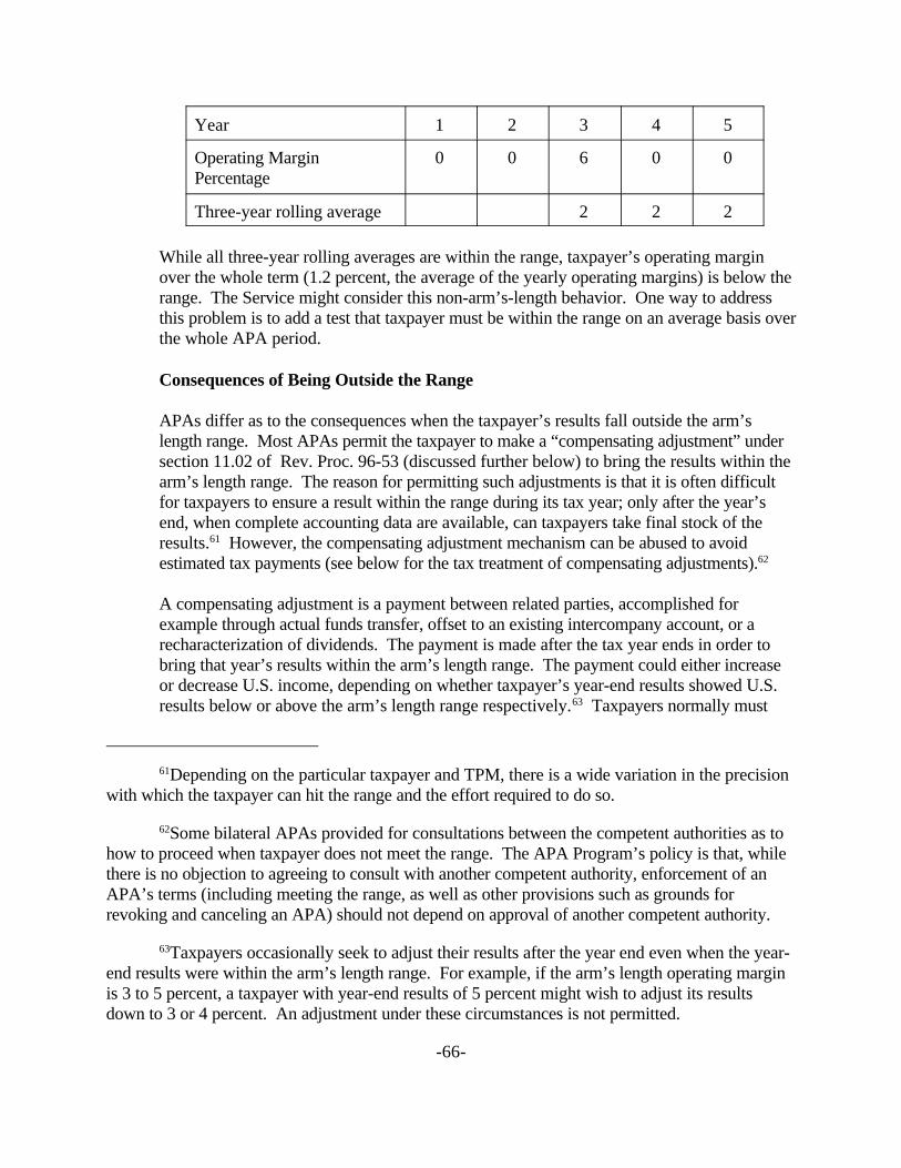
61Depending on the particular taxpayer and TPM, there is a wide variation in the precisionwith which the taxpayer can hit the range and the effort required to do so.

62Some bilateral APAs provided for consultations between the competent authorities as tohow to proceed when taxpayer does not meet the range. The APA Program’s policy is that, whilethere is no objection to agreeing to consult with another competent authority, enforcement of anAPA’s terms (including meeting the range, as well as other provisions such as grounds forrevoking and canceling an APA) should not depend on approval of another competent authority.

63Taxpayers occasionally seek to adjust their results after the year end even when the year-end results were within the arm’s length range. For example, if the arm’s length operating marginis 3 to 5 percent, a taxpayer with year-end results of 5 percent might wish to adjust its resultsdown to 3 or 4 percent. An adjustment under these circumstances is not permitted.

-66-

Year 1 2 3 4 5

Operating MarginPercentage

0 0 6 0 0

Three-year rolling average 2 2 2

While all three-year rolling averages are within the range, taxpayer’s operating marginover the whole term (1.2 percent, the average of the yearly operating margins) is below therange. The Service might consider this non-arm’s-length behavior. One way to addressthis problem is to add a test that taxpayer must be within the range on an average basis overthe whole APA period.

Consequences of Being Outside the Range

APAs differ as to the consequences when the taxpayer’s results fall outside the arm’slength range. Most APAs permit the taxpayer to make a “compensating adjustment” undersection 11.02 of Rev. Proc. 96-53 (discussed further below) to bring the results within thearm’s length range. The reason for permitting such adjustments is that it is often difficultfor taxpayers to ensure a result within the range during its tax year; only after the year’send, when complete accounting data are available, can taxpayers take final stock of theresults.61 However, the compensating adjustment mechanism can be abused to avoidestimated tax payments (see below for the tax treatment of compensating adjustments).62

A compensating adjustment is a payment between related parties, accomplished forexample through actual funds transfer, offset to an existing intercompany account, or arecharacterization of dividends. The payment is made after the tax year ends in order tobring that year’s results within the arm’s length range. The payment could either increaseor decrease U.S. income, depending on whether taxpayer’s year-end results showed U.S.results below or above the arm’s length range respectively.63 Taxpayers normally must

64The rationale for this distinction may be as follows. When the full range is used, thecomparables are of high reliability, such that the arithmetic mean of the results is the best point tochoose. When the interquartile range is used, the comparables are of lesser reliability, so somecomparables may be inappropriate outliers. Using the median instead of the arithmetic meandecreases the effect of those outliers.

-67-

make compensating adjustments within 90 days of the due date of the tax return (withextensions) for the year in question, but an APA can provide for a different deadline. If thedeadline is met, then no interest is paid or accrued on the intercompany amount due, and thetransfer is deemed for estimated tax purposes to occur on the last day of the tax year. (Thefavorable estimated tax treatment of compensating adjustments is intended to avoidpenalizing taxpayers that despite good faith efforts did not come within the range during thetax year.) However, there is no waiver of any interest due on additional tax owed as aresult of the compensating adjustment.

Precisely what adjustment is made? Under Reg. § 1.482–1(e)(3), if a taxpayer’s resultsfall outside the arm’s length range, the Service may adjust the result “to any point withinthe arm’s length range.” Accordingly, an APA may permit or require a taxpayer and itsrelated parties to make an adjustment after the year’s end to put the year’s results within therange, or at the point, specified by the APA. Similarly, to enforce the terms of an APA, theService may make such an adjustment.

Of the APAs that involve a range rather than a point, some provide for adjustment to theclosest edge of the range. This approach, normally sought by taxpayers, does not penalizea taxpayer for missing the range. Some APAs provide for adjustment to the median orsome other point within the range. An adjustment to the median, for example, candiscourage taxpayers from aiming for the very edge of the range, since if they miss therange they will be put at the median. An adjustment to the median also can discouragedeliberate missing of the range in an abuse of the compensating adjustment mechanism. Reg. § 1.482–1(e)(3) states that the adjustment is “ordinarily” to the median of thecomparables’ results when the interquartile range is used, and to the arithmetic mean of thecomparables’ results when the full range is used.64

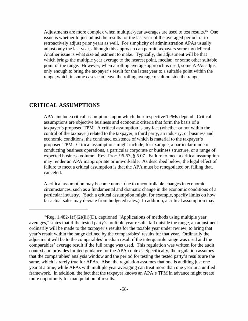
65Reg. 1.482-1(f)(2)(iii)(D), captioned “Applications of methods using multiple yearaverages,” states that if the tested party’s multiple year results fall outside the range, an adjustmentordinarily will be made to the taxpayer’s results for the taxable year under review, to bring thatyear’s result within the range defined by the comparables’ results for that year. Ordinarily theadjustment will be to the comparables’ median result if the interquartile range was used and thecomparables’ average result if the full range was used. This regulation was written for the auditcontext and provides limited guidance for the APA context. Specifically, the regulation assumesthat the comparables’ analysis window and the period for testing the tested party’s results are thesame, which is rarely true for APAs. Also, the regulation assumes that one is auditing just oneyear at a time, while APAs with multiple year averaging can treat more than one year in a unifiedframework. In addition, the fact that the taxpayer knows an APA’s TPM in advance might createmore opportunity for manipulation of results.

-68-

Adjustments are more complex when multiple-year averages are used to test results.65 Oneissue is whether to just adjust the results for the last year of the averaged period, or toretroactively adjust prior years as well. For simplicity of administration APAs usuallyadjust only the last year, although this approach can permit taxpayers some tax deferral. Another issue is what size adjustment to make. Typically, the adjustment will be thatwhich brings the multiple year average to the nearest point, median, or some other suitablepoint of the range. However, when a rolling average approach is used, some APAs adjustonly enough to bring the taxpayer’s result for the latest year to a suitable point within therange, which in some cases can leave the rolling average result outside the range.

CRITICAL ASSUMPTIONS

APAs include critical assumptions upon which their respective TPMs depend. Criticalassumptions are objective business and economic criteria that form the basis of ataxpayer’s proposed TPM. A critical assumption is any fact (whether or not within thecontrol of the taxpayer) related to the taxpayer, a third party, an industry, or business andeconomic conditions, the continued existence of which is material to the taxpayer’sproposed TPM. Critical assumptions might include, for example, a particular mode ofconducting business operations, a particular corporate or business structure, or a range ofexpected business volume. Rev. Proc. 96-53, § 5.07. Failure to meet a critical assumptionmay render an APA inappropriate or unworkable. As described below, the legal effect offailure to meet a critical assumption is that the APA must be renegotiated or, failing that,canceled.

A critical assumption may become unmet due to uncontrollable changes in economiccircumstances, such as a fundamental and dramatic change in the economic conditions of aparticular industry. (Such a critical assumption might, for example, specify limits on howfar actual sales may deviate from budgeted sales.) In addition, a critical assumption may

66Some past APAs took this approach but mislabeled the adjustment to the range as acritical assumption. This practice should be avoided since it can cause confusion and couldprovide the taxpayer grounds to argue for cancellation.

-69-

become unmet due to a taxpayer’s actions that are initiated for good faith business reasons,such as a change in business strategy, mode of conducting operations, or the cessation ortransfer of a business segment or entity covered by the APA.

Guidelines for Avoiding Problems with Critical Assumptions

1. Make critical assumptions extreme outer limits. Then, if they are unmet, thingshave changed so much that cancellation would be appropriate. Also, taxpayerswill be less able to manipulate a failure of the assumption. Finally, with thisapproach critical assumptions will not fail so much. It is a shame to conclude anAPA after much effort, only to be back at the negotiating table after a criticalassumption fails.

2. When possible, make critical assumptions objective. Critical assumptions canrefer to either subjective conditions (e.g., material changes in a business) orobjective (e.g., sales dropping by a certain percentage). The standard criticalassumption given below is subjective. However, when possible, make othercritical assumptions objective. For example, refer to sales dropping by a definitepercentage rather than sales dropping “substantially.” This practice will avoiddisputes over whether the terms of a critical assumption were met.

3. Try to use TPM provisions rather than critical assumptions. For example,instead of having a critical assumption that sales not fluctuate too much frombudgeted amounts, it might be possible instead to provide that such fluctuations willcause certain adjustments to the range.66 As another example, suppose that an APAuses a CPM with a gross margin PLI for a U.S. distributor. The Service may beconcerned that the distributor will make excessive advertising expenditures withoutreimbursement from the parent, with the effect of building up the parent’s marketingintangibles. (Such expenditures would not affect gross margin, and thus would notcause the distributor to fall outside an agreed gross margin range.) Instead ofincluding a critical assumption that advertising expenses must be within a certainlevel, one could specify that for purposes of computing the distributor’s gross profitlevel during the APA years, advertising expenses above a certain amount will besubtracted from sales.

4. Do not confuse critical assumptions with the scope of the APA. For example, anAPA may specify that new product types will not be covered. This provisionshould be part of the definition of covered transactions; the APA should not includea critical assumption that new products not be introduced.

-70-

5. Do not confuse critical assumptions with obligations of the taxpayer. Forexample, an APA may require a taxpayer to record certain information in aregularly compiled database. (This requirement could be put in an additionalparagraph in the text of the APA, with language clearly stating that taxpayer wascommitting to this obligation as an express term of the APA.) If the taxpayer doesnot do so, the taxpayer has violated the terms and conditions of the APA, whichgives the Service the option to either enforce or cancel/revoke the APA. Thisobligation of the taxpayer is not a critical assumption and should not be so labeled.

Effects of Not Meeting Critical Assumptions

If a critical assumption has not been met, the taxpayer must notify the Service. (However,the Service itself may determine whether a critical assumption is met, perhaps usinginformation gained on examination.) The parties may agree on certain revisions of theAPA, or may agree to keep the APA the same despite the failure of the critical assumption. (For bilateral cases, the foreign competent authority will be consulted, but in absence ofagreement by the foreign competent authority the Service and the taxpayer can still reach anagreement.) If the parties cannot agree how to handle the failure of the critical assumption,the APA is canceled. Rev. Proc. 96–53, § 11.07.

Standard Critical Assumption

Included in the model APA is the following critical assumption (this language is subject torevision):

The business activities, functions performed, risks assumed, assets employed, andfinancial [and tax] accounting methods and categories [and estimates] of Taxpayershall remain materially the same as described in Taxpayer’s request for this APA.

Taxpayer Specific Critical Assumptions

The APAs concluded as of December 31, 1999, included approximately 160 differentcritical assumptions in addition to the model APA critical assumption noted above. Manyof these critical assumptions appear in more than one APA. Most of the criticalassumptions reflect specific terms and factors of each taxpayer in an elaboration of thegeneral model APA critical assumption. The critical assumptions have not alwaysfollowed the guidelines given above.

The critical assumptions can be subdivided into the following categories, discussed furtherbelow:

(i) operational(ii) legal(iii) tax

-71-

(iv) financial(v) accounting(vi) economic

Operational Critical Assumptions

Over 100 critical assumptions fell into the operational category. Over twenty involvedcosts or expenses, such as how the taxpayer defines, computes, allocates, and apportionscosts and expenses, and limits on the amount and manner by which expenses and costs canvary. An example is that a U.S. subsidiary’s deductions for restructuring fees shall notexceed a stated maximum dollar amount.

Six operational critical assumptions involved sales. These concern limits on sales mixes,maximum sales amounts, projections of sales, and permissible sales trends and variations. An example of this type of critical assumption is that the combined sales of coveredproducts for each APA year must be within 20% of the previous year.

Five operational critical assumptions involved permissible variations in items other thansales or expenses. These include how new or disposed of affiliates are treated, to whatextent inventories can fluctuate, or to what extent covered purchases can be importedfinished products. An example of this type of critical assumption is that the share ofcovered products that are imported finished goods can vary by X% from the historicalbaseline share percentage of imported finished goods.

The rest involved other limits on change. These critical assumptions state in a specificway that the following items remain substantially the same: customers, products, risks,functions, business methods, assets, pricing policies, absence of catastrophic events,business structure, presence and effect of a cost sharing agreement, functional currency,operating assets, presence or absence of intangible assets, intangible asset ownership,parties to the agreement, licensee agreements, specific personnel, location of specificpersonnel, presence or absence of commissions, and royalty amounts and percentages. Anexample of this type of critical assumption is that the location of a particular key executivemay not change.

Legal Critical Assumptions

Fourteen critical assumptions involved legal issues. They include the nature and scope ofcompetent authority agreements. An example is that the competent authorities’ mutualagreement, which is conditioned on the system profit remaining above a specified minimumlevel, will remain in effect (i.e., that such condition will continue to be satisfied).

Other critical assumptions of this nature involved liquidations, dissolutions, customs lawchanges, major regulatory changes, new import or export barriers, and maintenance of adistributor agreement in a specific form. An example of this type of critical assumption isthat customs duties on imported covered products shall not vary beyond certain limits.

67It probably would have been better not to have a critical assumption for this, but insteadto state that the taxpayer had an obligation to keep the statute of limitations open. See Guideline 5above.

68It may have been more appropriate to recast some of these critical assumptions as TPMprovisions. See Guideline 3 above.

69Many of these critical assumptions probably could have been expressed instead as anobligation of the taxpayer. See Guideline 5 above.

-72-

Others involved which controlled entity has title to inventory and production equipment, orwhich controlled entity is required to maintain guarantees, warranties, or product liability. An example of this type of critical assumption is that a parent corporation must maintainexisting guarantees for all liabilities of its subsidiary, including its debt and productliability guarantees.

Tax Critical Assumptions

Eleven critical assumptions involved tax issues. These issues include estimated taxliability, period of limitation on assessment, tax effect of specified expenses, sourcing ofincome, Subpart F income, permanent establishment, foreign tax credit limitation,increasing coverage to other controlled foreign corporations, the ability to change aspecified tax election, ability to file for a refund, and a condition of subsequently enteringinto a closing agreement for rollback years. An example of this type of critical assumptionis that the period of limitation on assessments shall be kept open for all APA years untilsuch period expires for the last APA year under U.S. tax law.67

Financial Critical Assumptions

Eighteen types of critical assumptions were financial in nature. These involve limitationson system loss, intangible profit projections, buy-in payments, lack of currency risk, andvalid business reason for debt. Also included in this category are a number ofrequirements for maintaining various financial ratios such as profit splits, Berry ratios,operating profit margins, and gross profit margins, within prescribed ranges or withinlimits. An example of this type of critical assumption is that the TPM may not yield a grossmargin outside A% to B% for a controlled subsidiary, nor may the combined operatingmargins be outside C% to D% for the parent and the subsidiary, unless due to validbusiness reasons or attributable to economic conditions beyond the parent’s control.68

Accounting Critical Assumptions

Seven critical assumptions involve accounting methods or practices.69 These includeassumptions regarding the use of generally accepted accounting principles, favorablecertified opinions, mark to market accounting, consistency of accounting computations for

-73-

all related parties, methods of accounting for foreign currency gains and losses, andunchanged methods for both financial and tax accounting. An example of this type ofcritical assumption is that manufacturing costs must be computed in the same manner byU.S. and foreign members of an affiliated group.

Economic Critical Assumptions

Eight critical assumptions involve economic and financial conditions. These includeassumptions regarding interest rates and changes in interest rates. They also includeassumptions that there will not be significant changes in market conditions, technology,product liability, product design, process design, and market share. An example of thistype of critical assumption is that there shall not be an unexpected economic developmentthat materially affects a company’s market share or market price of a covered product.

-i- apa study guide lesson one: major elements

Documents