© eric xing @ cmu, 2006-20101 machine learning generative verses discriminative classifier eric...

© Eric Xing @ CMU, 2006-2010 1

Machine LearningMachine Learning

Generative verses discriminative Generative verses discriminative classifier classifier

Eric XingEric Xing

Lecture 2, August 12, 2010

Reading:

© Eric Xing @ CMU, 2006-2010 2

Generative and Discriminative classifiers

Goal: Wish to learn f: X Y, e.g., P(Y|X)

Generative: Modeling the joint distribution

of all data

Discriminative: Modeling only points

at the boundary

© Eric Xing @ CMU, 2006-2010 3

Generative vs. Discriminative Classifiers


Generative classifiers (e.g., Naïve Bayes): Assume some functional form for P(X|Y), P(Y)

This is a ‘generative’ model of the data! Estimate parameters of P(X|Y), P(Y) directly from training data Use Bayes rule to calculate P(Y|X= x)

Discriminative classifiers (e.g., logistic regression) Directly assume some functional form for P(Y|X)

This is a ‘discriminative’ model of the data! Estimate parameters of P(Y|X) directly from training data

Yn

Xn

Yn

Xn

© Eric Xing @ CMU, 2006-2010 4

Suppose you know the following …

Class-specific Dist.: P(X|Y)

Class prior (i.e., "weight"): P(Y)

This is a generative model of the data!

),;(

)|(

111

1

Xp

YXp

),;(

)|(

222

2

Xp

YXp

Bayes classifier:

© Eric Xing @ CMU, 2006-2010 5

Optimal classification

Theorem: Bayes classifier is optimal!

That is

How to learn a Bayes classifier? Recall density estimation. We need to estimate P(X|y=k), and P(y=k) for all k

© Eric Xing @ CMU, 2006-2010 6

Gaussian Discriminative Analysis

learning f: X Y, where X is a vector of real-valued features, Xn= < Xn,1…Xn,m >

Y is an indicator vector

What does that imply about the form of P(Y|X)? The joint probability of a datum and its label is:

Given a datum xn, we predict its label using the conditional probability of the label given the datum:

Yn

Xn

2

21

2/12)-(-exp

)2(

1

),,1|()1(),|1,(

2 knk

knn

kn

knn ypypyp

x

xx

'

2'2

12/12'

2

21

2/12

)(exp)2(

1

)(exp)2(

1

),,|1(

2

2

kknk

knk

nknyp

x

x

x

© Eric Xing @ CMU, 2006-2010 7

Conditional Independence

X is conditionally independent of Y given Z, if the probability distribution governing X is independent of the value of Y, given the value of Z

Which we often write

e.g.,

Equivalent to:

© Eric Xing @ CMU, 2006-2010 8

Naïve Bayes Classifier

When X is multivariate-Gaussian vector: The joint probability of a datum and it label is:

The naïve Bayes simplification

More generally:

Where p(. | .) is an arbitrary conditional (discrete or continuous) 1-D density

)-()-(-exp)2(

1

),,1|()1(),|1,(

121

2/1 knT

knk

knn

kn

knn ypypyp

xx

xx

Yn

Xn

jjkjn

jkk

jjkjk

knjn

kn

knn

x

yxpypyp

jk

2,,2

12/12

,

,,,

)-(-exp)2(

1

),,1|()1(),|1,(

2,

x

m

jnjnnnn yxpypyp

1, ),|()|(),|,( x

Yn

Xn,1 Xn,2 Xn,m…

© Eric Xing @ CMU, 2006-2010 9

The predictive distribution

Understanding the predictive distribution

Under naïve Bayes assumption:

For two class (i.e., K=2), and when the two classes haves the same variance, ** turns out to be a logistic function

* ),|,(

),|,(

),|(

),,|,(),,,|(

' '''

k kknk

kknk

n

nkn

nkn xN

xN

xp

xypxyp

1

1

1

1222

1221

1

2222

12

1221

121

11

1

1

1

)(2

log)-(exp

log)-(exp

log)][-]([)-(exp

j

jjjjjnCx

Cx

jjj jjj

nj

j jjj

nj

x

nT xe

1

1

)|( nn xyp 11

**

log)(exp

log)(exp

),,,|(

' ,'','

'

,,

k j jkj

kj

njk

k

j jkj

kj

njk

k

nkn

Cx

Cx

xyp

2

2

22

21

21

1

© Eric Xing @ CMU, 2006-2010 10

The decision boundary

The predictive distribution

The Bayes decision rule:

For multiple class (i.e., K>2), * correspond to a softmax function

j

x

x

nkn

nTj

nTk

e

exyp

)|( 1

nT xM

j

jnj

nne

x

xyp

1

1

1

11

01

1

exp

)|(

nT

x

x

x

nn

nn x

e

ee

xyp

xyp

nT

nT

nT

1

1

1

11

2

1 ln

)|(

)|(ln

© Eric Xing @ CMU, 2006-2010 11





Discriminative classifiers: Directly assume some functional form for P(Y|X)


Yi

Xi

Yi

Xi

© Eric Xing @ CMU, 2006-2010 12

Linear Regression

The data:

Both nodes are observed: X is an input vector Y is a response vector

(we first consider y as a generic

continuous response vector, then

we consider the special case of

classification where y is a discrete

indicator)

A regression scheme can be

used to model p(y|x) directly,

rather than p(x,y)

Yi

Xi

N

),(,),,(),,(),,( NN yxyxyxyx 332211

© Eric Xing @ CMU, 2006-2010 13

Linear Regression

Assume that Y (target) is a linear function of X (features): e.g.:

let's assume a vacuous "feature" X0=1 (this is the intercept term, why?), and define the feature vector to be:

then we have the following general representation of the linear function:

Our goal is to pick the optimal . How! We seek that minimize the following cost function:

n

iiii yxyJ

1

2

21

))(ˆ()(

© Eric Xing @ CMU, 2006-2010 14

The Least-Mean-Square (LMS) method

Consider a gradient descent algorithm:

Now we have the following descent rule:

For a single training point, we have:

This is known as the LMS update rule, or the Widrow-Hoff learning rule This is actually a "stochastic", "coordinate" descent algorithm This can be used as a on-line algorithm

n

i

ji

tTii

tj

tj xy

1

1 )( x

ji

tTii

tj

tj xy )(1 x

tj

tj

tj J )(

1

© Eric Xing @ CMU, 2006-2010 15

Probabilistic Interpretation of LMS

Let us assume that the target variable and the inputs are related by the equation:

where ε is an error term of unmodeled effects or random noise

Now assume that ε follows a Gaussian N(0,σ), then we have:

By independence assumption:

iiT

iy x

2

2

22

1

)(

exp);|( iT

iii

yxyp

x

2

1

2

1 22

1

n

i iT

inn

iii

yxypL

)(exp);|()(

x

© Eric Xing @ CMU, 2006-2010 16

Probabilistic Interpretation of LMS, cont.

Hence the log-likelihood is:

Do you recognize the last term?

Yes it is:

Thus under independence assumption, LMS is equivalent to MLE of θ !

n

i iT

iynl1

22 2

11

2

1)(log)( x

n

ii

Ti yJ

1

2

21

)()( x

© Eric Xing @ CMU, 2006-2010 17

Classification and logistic regression

© Eric Xing @ CMU, 2006-2010 18

The logistic function

© Eric Xing @ CMU, 2006-2010 19

Logistic regression (sigmoid classifier)

The condition distribution: a Bernoulli

where is a logistic function

We can used the brute-force gradient method as in LR

But we can also apply generic laws by observing the p(y|x) is an exponential family function, more specifically, a generalized linear model (see future lectures …)

yy xxxyp 11 ))(()()|(

xT

ex

1

1)(

© Eric Xing @ CMU, 2006-2010 20

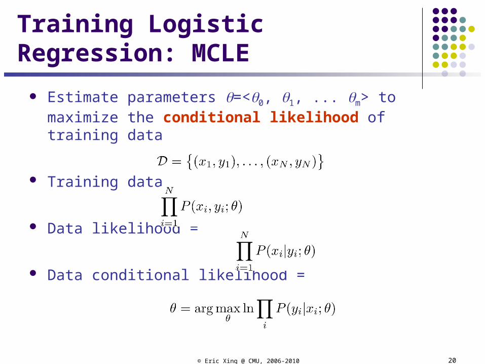
Training Logistic Regression: MCLE

Estimate parameters =<0, 1, ... m> to maximize the conditional likelihood of training data

Training data

Data likelihood =

Data conditional likelihood =

© Eric Xing @ CMU, 2006-2010 21

Expressing Conditional Log Likelihood

Recall the logistic function:

and conditional likelihood:

© Eric Xing @ CMU, 2006-2010 22

Maximizing Conditional Log Likelihood

The objective:

Good news: l() is concave function of

Bad news: no closed-form solution to maximize l()

© Eric Xing @ CMU, 2006-2010 23

The Newton’s method

Finding a zero of a function

© Eric Xing @ CMU, 2006-2010 24

The Newton’s method (con’d)

To maximize the conditional likelihood l():

since l is convex, we need to find where l’()=0 !

So we can perform the following iteration:

© Eric Xing @ CMU, 2006-2010 25

The Newton-Raphson method

In LR the is vector-valued, thus we need the following generalization:

is the gradient operator over the function

H is known as the Hessian of the function

© Eric Xing @ CMU, 2006-2010 26

The Newton-Raphson method

In LR the is vector-valued, thus we need the following generalization:

is the gradient operator over the function

H is known as the Hessian of the function

© Eric Xing @ CMU, 2006-2010 27

Iterative reweighed least squares (IRLS)

Recall in the least square est. in linear regression, we have:

which can also derived from Newton-Raphson

Now for logistic regression:

© Eric Xing @ CMU, 2006-2010 28





Discriminative classifiers: Directly assume some functional form for P(Y|X)


Yi

Xi

Yi

Xi

© Eric Xing @ CMU, 2006-2010 29

Naïve Bayes vs Logistic Regression

Consider Y boolean, X continuous, X=<X1 ... Xm> Number of parameters to estimate:

NB:

LR:

Estimation method: NB parameter estimates are uncoupled LR parameter estimates are coupled

**

log)(2

1exp

log)(2

1exp

)|(

' ,'2

,'2,'

'

,2

,2,

k j jkjkjjk

k

j jkjkjjk

k

Cx

Cx

yp

x

xT

ex

1

1)(

© Eric Xing @ CMU, 2006-2010 30


Asymptotic comparison (# training examples infinity)

when model assumptions correct NB, LR produce identical classifiers

when model assumptions incorrect LR is less biased – does not assume conditional independence therefore expected to outperform NB

© Eric Xing @ CMU, 2006-2010 31


Non-asymptotic analysis (see [Ng & Jordan, 2002] )

convergence rate of parameter estimates – how many training examples needed to assure good estimates?

NB order log m (where m = # of attributes in X)

LR order m

NB converges more quickly to its (perhaps less helpful) asymptotic estimates

© Eric Xing @ CMU, 2006-2010 32

Some experiments from UCI data sets

© Eric Xing @ CMU, 2006-2010 33

Robustness

• The best fit from a quadratic regression

• But this is probably better …

© Eric Xing @ CMU, 2006-2010 34

Bayesian Parameter Estimation

Treat the distribution parameters also as a random variable The a posteriori distribution of after seem the data is:

This is Bayes Rule

likelihood marginal

priorlikelihoodposterior

dpDp

pDp

Dp

pDpDp

)()|(

)()|(

)(

)()|()|(

The prior p(.) encodes our prior knowledge about the domain

© Eric Xing @ CMU, 2006-2010 35

35

What if is not invertible ?

log likelihood log prior

Prior belief that β is Gaussian with zero-mean biases solution to “small” β

I) Gaussian Prior

0

Ridge Regression

Closed form: HW

Regularized Least Squares and MAP

© Eric Xing @ CMU, 2006-2010 36

Regularized Least Squares and MAP

36

What if is not invertible ?

log likelihood log prior

Prior belief that β is Laplace with zero-mean biases solution to “small” β

Lasso

Closed form: HW

II) Laplace Prior

© Eric Xing @ CMU, 2006-2010 37

Ridge Regression vs Lasso

37

Ridge Regression: Lasso: HOT!

Lasso (l1 penalty) results in sparse solutions – vector with more zero coordinatesGood for high-dimensional problems – don’t have to store all coordinates!

βs with constant l1 norm

βs with constant J(β)(level sets of J(β))

βs with constant l2 norm

β2

β1

© Eric Xing @ CMU, 2006-2010 38

Case study: predicting gene expression

The genetic picture

CGTTTCACTGTACAATTT

causal SNPscausal SNPs

a univariate phenotype:a univariate phenotype:

i.e., the expression intensity of i.e., the expression intensity of a genea gene

© Eric Xing @ CMU, 2006-2010 39

Individual 1

Individual 2

Individual N

Phenotype (BMI)

2.5

4.8

4.7

Genotype

. . C . . . . . T . . C . . . . . . . T . . .

. . C . . . . . A . . C . . . . . . . T . . .

. . G . . . . . A . . G . . . . . . . A . . .

. . C . . . . . T . . C . . . . . . . T . . .

. . G . . . . . T . . C . . . . . . . T . . .

. . G . . . . . T . . G . . . . . . . T . . .

Causal SNPBenign SNPs

…

Association Mapping as Regression

© Eric Xing @ CMU, 2006-2010 40© Eric Xing @ CMU, 2006-2008 40

Individual 1

Individual 2

Individual N

Phenotype (BMI)

2.5

4.8

4.7

Genotype

. . 0 . . . . . 1 . . 0 . . . . . . . 0 . . .

. . 1 . . . . . 1 . . 1 . . . . . . . 1 . . .

. . 2 . . . . . 2 . . 1 . . . . . . . 0 . . .

…

yi =

J

jjijx

1

SNPs with large |βj| are relevant

Association Mapping as Regression


Experimental setup

Asthama dataset 543 individuals, genotyped at 34 SNPs Diploid data was transformed into 0/1 (for homozygotes) or 2 (for heterozygotes) X=543x34 matrix Y=Phenotype variable (continuous)

A single phenotype was used for regression

Implementation details Iterative methods: Batch update and online update implemented. For both methods, step size α is chosen to be a small fixed value (10-6). This

choice is based on the data used for experiments. Both methods are only run to a maximum of 2000 epochs or until the change in

training MSE is less than 10-4


For the batch method, the training MSE is initially large due to uninformed initialization In the online update, N updates for every epoch reduces MSE to a much smaller value.

Convergence Curves


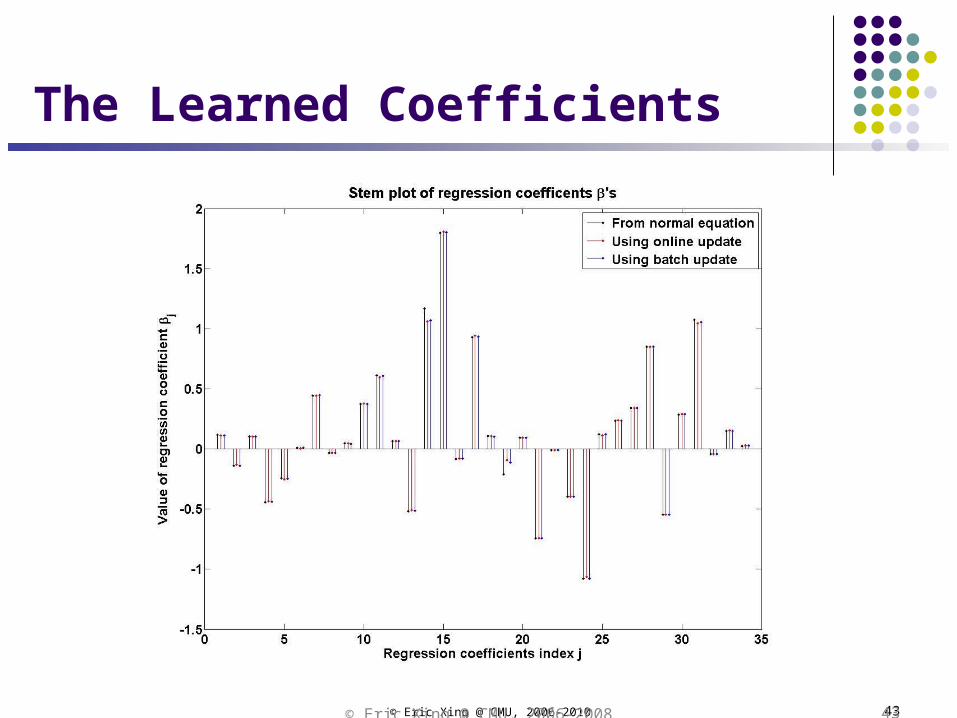
The Learned Coefficients


The results from B and O update are almost identical. So the plots coincide.

The test MSE from the normal equation is more than that of B and O during small training. This is probably due to overfitting.

In B and O, since only 2000 iterations are allowed at most. This roughly acts as a mechanism that avoids overfitting.

Performance vs. Training Size

© Eric Xing @ CMU, 2006-2010 45

Summary

Naïve Bayes classifier What’s the assumption Why we use it How do we learn it

Logistic regression Functional form follows from Naïve Bayes assumptions For Gaussian Naïve Bayes assuming variance For discrete-valued Naïve Bayes too But training procedure picks parameters without the conditional independence

assumption

Gradient ascent/descent – General approach when closed-form solutions unavailable

Generative vs. Discriminative classifiers – Bias vs. variance tradeoff

© Eric Xing @ CMU, 2006-2010 47

Parameter Learning from iid Data

Goal: estimate distribution parameters from a dataset of N independent, identically distributed (iid), fully observed, training cases

D = {x1, . . . , xN}

Maximum likelihood estimation (MLE)1. One of the most common estimators

2. With iid and full-observability assumption, write L() as the likelihood of the data:

3. pick the setting of parameters most likely to have generated the data we saw:

);,,()( , NxxxPL 21

N

i i

N

xP

xPxPxP

1

2

);(

);(,),;();(

)(maxarg*

L )(logmaxarg

L

© Eric Xing @ CMU, 2006-2010 48

Example: Bernoulli model

Data: We observed N iid coin tossing: D={1, 0, 1, …, 0}

Representation:

Binary r.v:

Model:

How to write the likelihood of a single observation xi ?

The likelihood of datasetD={x1, …,xN}:

ii xxixP 11 )()(

N

i

xxN

iiN

iixPxxxP1

1

121 1 )()|()|,...,,(

},{ 10nx

tails#head# )()(

11 11

1N

ii

N

ii xx

1

01

x

xxP

for

for )(

xxxP 11 )()(

© Eric Xing @ CMU, 2006-2010 49

Maximum Likelihood Estimation

Objective function:

We need to maximize this w.r.t.

Take derivatives wrt

Sufficient statistics The counts, are sufficient statistics of data D

)log()(log)(log)|(log);( 11 hhnn nNnDPD thl

01

hh nNnl

N

nhMLE

i

iMLE xN

1

or

Frequency as sample mean

, where, i ikh xnn

© Eric Xing @ CMU, 2006-2010 50

Overfitting

Recall that for Bernoulli Distribution, we have

What if we tossed too few times so that we saw zero head?

We have and we will predict that the probability of seeing a head next is zero!!!

The rescue: "smoothing" Where n' is know as the pseudo- (imaginary) count

But can we make this more formal?

tailhead

headheadML nn

n

,0headML

'

'

nnnnn

tailhead

headheadML

© Eric Xing @ CMU, 2006-2010 51

Bayesian Parameter Estimation

Treat the distribution parameters also as a random variable The a posteriori distribution of after seem the data is:

This is Bayes Rule

likelihood marginal

priorlikelihoodposterior

dpDp

pDp

Dp

pDpDp

)()|(

)()|(

)(

)()|()|(

The prior p(.) encodes our prior knowledge about the domain

© Eric Xing @ CMU, 2006-2010 52

Frequentist Parameter Estimation

Two people with different priors p() will end up with different estimates p(|D).

Frequentists dislike this “subjectivity”. Frequentists think of the parameter as a fixed, unknown

constant, not a random variable. Hence they have to come up with different "objective"

estimators (ways of computing from data), instead of using Bayes’ rule. These estimators have different properties, such as being “unbiased”, “minimum

variance”, etc. The maximum likelihood estimator, is one such estimator.

© Eric Xing @ CMU, 2006-2010 54

Bayesian estimation for Bernoulli

Beta distribution:

When x is discrete

Posterior distribution of :

Notice the isomorphism of the posterior to the prior, such a prior is called a conjugate prior and are hyperparameters (parameters of the prior) and correspond to the

number of “virtual” heads/tails (pseudo counts)

1111

1

11 111 thth nnnn

N

NN xxp

pxxpxxP )()()(

),...,(

)()|,...,(),...,|(

1111 11

)(),()(

)()(

)(),;( BP

!)()( xxxx 1

© Eric Xing @ CMU, 2006-2010 55

Bayesian estimation for Bernoulli, con'd

Posterior distribution of :

Maximum a posteriori (MAP) estimation:

Posterior mean estimation:

Prior strength: A=+ A can be interoperated as the size of an imaginary data set from which we obtain the

pseudo-counts

1111

1

11 111 thth nnnn

N

NN xxp

pxxpxxP )()()(

),...,(

)()|,...,(),...,|(

N

ndCdDp hnn

Bayesth 11 1 )()|(

Bata parameters can be understood as pseudo-counts

),...,|(logmaxarg NMAP xxP 1

© Eric Xing @ CMU, 2006-2010 56

Effect of Prior Strength

Suppose we have a uniform prior (==1/2),

and we observe Weak prior A = 2. Posterior prediction:

Strong prior A = 20. Posterior prediction:

However, if we have enough data, it washes away the prior. e.g., . Then the estimates under weak and strong prior are and , respectively, both of which are close to 0.2

),( 82 th nnn

25010221

282 .)',,|(

th nnhxp

4001020210

2082 .)',,|(

th nnhxp

),( 800200 th nnn

100022001

10002020010

© Eric Xing @ CMU, 2006-2010 57

Example 2: Gaussian density

Data: We observed N iid real samples:

D={-0.1, 10, 1, -5.2, …, 3}

Model:

Log likelihood:

MLE: take derivative and set to zero:

22212 22 /)(exp)(/

xxP

N

n

nxNDPD

12

22

21

22

)log()|(log);(l

n n

n n

xN

x

2

422

2

21

2

1

l

l)/(

n MLnMLE

n nMLE

xN

xN

22 1

1

© Eric Xing @ CMU, 2006-2010 58

MLE for a multivariate-Gaussian

It can be shown that the MLE for µ and Σ is

where the scatter matrix is

The sufficient statistics are nxn and nxnxnT.

Note that XTX=nxnxnT may not be full rank (eg. if N <D), in which case ΣML is not

invertible

SN

xxN

xN

n

TMLnMLnMLE

n nMLE

11

1

TMLMLn n

Tnnn

TMLnMLn NxxxxS

Kn

n

n

n

x

x

x

x

2

1

TN

T

T

x

x

x

X2

1

© Eric Xing @ CMU, 2006-2010 59

Bayesian estimation

Normal Prior:

Joint probability:

Posterior:

20

20

2120 22 /)(exp)(

/

P

1

20

22

020

2

20

20

2

2 11

11

N

Nx

N

N ~ and , //

/

//

/~ where

Sample mean

20

20

2120

1

2

2

22

22

21

2

/)(exp

exp),(

/

/

N

nn

NxxP

22212 22 ~/)~(exp~)|(/

xP

© Eric Xing @ CMU, 2006-2010 60

Bayesian estimation: unknown µ, known σ

The posterior mean is a convex combination of the prior and the MLE, with weights proportional to the relative noise levels.

The precision of the posterior 1/σ2N is the precision of the prior 1/σ2

0 plus one contribution of data precision 1/σ2 for each observed data point.

Sequentially updating the mean µ ∗ = 0.8 (unknown), (σ2) ∗ = 0.1 (known)

Effect of single data point

Uninformative (vague/ flat) prior, σ20 →∞

1

20

22

020

2

20

20

2

2 11

11

N

Nx

N

NN

~ , //

/

//

/

20

2

20

020

2

20

001

)( )( xxx

0 N

© eric xing @ cmu, 2006-20101 machine learning generative verses discriminative classifier eric...

Documents