Jurnal Kejuruteraan 7 (1995) 19-31

Theoretical Evaluation of Dynamic Creep Modulus of Bituminous Concrete and Comparison with

Experimental Results

Shakor R Badaruddin

ABSTRACT

Knowledge of bituminous creep modulus is very importan! to fully characterize a premix. Conventional methods to determine it involve elaborate laboratory procedure requiring specialized equipment and trained personnel. Theoretical methods. to calculate dynamic creep modulus (E*) have been available bur very little comparison between theoretical and laboratory results are available in the literature. A study was carried out to determine the laboratory E* values of a ser of field cores. The same cores were then analyzed for rheir physical properties such as penetration. viscosity and air-void content which were used as input for the determination of the theoretical E*. A comparison was then made between rhe laboratory and theoretical E* values in graphical plots which showed agreement within a factor two. In many analysis, this is close enough given the inherent variability within a premix. Thus. in cases where laboratory E* could not be performed. a quick esrimate could be obtained using the method shawn in this srudy.

ABSTRAK

Pengetahuan mengenai modulus rayapan bitumen adalah penting dalam mencirikan pracampuran. Penentuannya dengan kaedah biasa melibatkan tatacara makmol tertentu yang memerlukan peralatan khusus dan kakilangan yang terlatih. Memang telah wujud kaelinh teori untuk menghirung modulus rayapan dinamik (E*). rerapi terlalu sedikit dilakukan perbandingan amara hasil teori dengan keputusan makmal. Suatu kajian lelah dilakukan un/uk menentukan ni/ai makmal bag; E* bag; suatu set sampel teras lapangan. Sampel reras yang sama kemudiannya dianalisis untuk mengerahui sifat­sifat fisikal seperti rusukan. kelikatan. dan kandungan lompang udara. yang digunakan sebagai nilai awal penentuan E* teori. Perbandingan kemudiannya dilakukan amara nilni-nilai E* malanal dan teori linlam suatu plot graf yang menunjukkan perserujuan dengan faktor 2. Dalam kebanyakan analisis. ini adalah memuaskan memandangkan kebolehubahan yang terwujud pada pracampuran. Oleh itu. dalam kes-kes yang mana nilai E* makmal tidak dapar diperolehi. anggaran yang cepar boleh diperolehi dengan kaedah yang ditunjukkan dalam kajian ini.

INTRODUCTION

Various characteristics of bituminous concrete must be known before its perfonnance can be predicted in the field. The basic test methods commonly available are rigorous laboratory ones comprising mainly of testing the ..

• 20

mixture like Marshall Stability, void content and testing the properties of mixture components namely the aggregates and the asphalt. These mixture characteristics which are used for mix design do not fully explain or rather govern the way the pavement will perform because mix design is an empirical procedure [I]. This is evident from the continuous problems faced by the pavement industry especially with regards to rutting and early failure [2]. Thus there has been an increasing attention towards investigating the complex material response, or the static and dynamic creep modulus when a simulated traffic load is applied to bituminous concrete (premix). As a result numerous studies have evolved [3, 4] which show that creep testing are valuable tools in characterizing pavement performance [3,5]. Dynamic creep test has been indicated to provide a better predicted response for highway pavements because the dynamic or repeated loading tests in the laboratory simulates traffic loading [5, 6].

Laboratory testing of dynamic creep however is a cumbersome procedure requiring skilled expertise and sophisticated equipmentation. Evaluation of dynamic creep theoretically without having to carry out the actual dynamic test would provide designers with a tool to improve pavement design more efficiently. In this paper a method is shown how to obtain the theoretical dynamic creep modulus for bituminous concrete mixtures which compares favorably with results of repeated loading tests in the laboratory on the same samples.

CONCEPT OF DYNAMIC CREEP MODULUS

Dynamic creep modulus of bituminous concrete (or premix), denoted by E*, is a simple variation of the Young's elastic modulus E due to it being no longer elastic; it is viscoelastic, comprising of a compacted matrix of elastic aggregates held together by a viscous binding agent, asphalt. Young's

p

~~ 1---4-------1 r -:- 1-,-I , I

: i : I I

: ; : L ..........•...................... , ................... ··1··········

I ' I I I I I I I I I I I

: j : , -----.;-----1-.

t FIGURE I. Typical Sample Deformation Under Load.

21

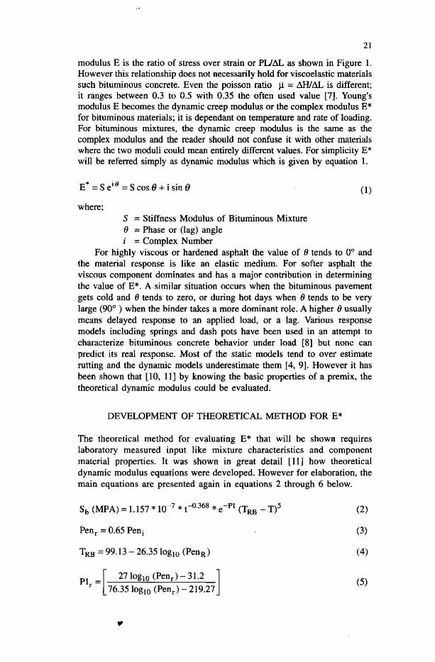
modulus E is the ratio of stress over strain or PUt.L as shown in Figure I. However this relationship does not necessarily hold for viscoelastic materials such bituminous concrete. Even the poisson ratio 11 = &l/t.L is different; it ranges between 0.3 to 0.5 with 0.35 the often used value [7]. Young's modulus E becomes the dynamic creep modulus or the complex modulus E* for bituminous materials; it is dependant on temperature and rate of loading. For bituminous mixtures, the dynamic creep modulus is the same as the complex modulus and the reader should not confuse it with other materials where the two moduli could mean entirely different values. For simplicity E* will be referred simply as dynamic modulus which is given by equation I.

E' = S e; 8 = S cos /I + i sin /I

where; S = Stiffness Modulus of Bituminous Mixture o = Phase or (lag) angle i = Complex Number

(I)

For highly viscous or hardened asphalt the value of 9 tends to 0° and the material response is like an elastic medium. For softer asphalt the viscous component dominates and has a major contribution in detennining the value of EO. A .similar situation occurs when the bituminous pavement gets cold and 9 tends to zero, or during hot days when 6 tends to be very large (90° ) when the binder takes a more dominant role. A higher 0 usually means delayed response to an applied load, or a lag. Various response models including springs and dash pots have been used in an attempt to characterize bituminous concrete behavior under load [8] but none can predict its real response. Most of the static models tend to over estimate rutting and the dynamic models underestimate them [4, 9]. However it has been shown that [10, ll] by knowing the basic properties of a premix, the theoretical dynamic modulus could be evaluated.

DEVELOPMENT OF THEORETICAL METHOD FOR E*

The theoretical method for evaluating E* that will be shown requires laboratory measured input like mixture characteristics and component material properties. It was shown in great detail [I I] how theoretical dynamic modulus equations were developed. However for elaboration, the main equations are presented again in equations 2 through 6 below.

Sb (MPA) = 1.157 * 10-7 * (-0.368. e-Pt (TRB _ T)5

Penr = 0.65 Pen;

TRB = 99.13 - 26.3510g lO (PenR)

PI = [ 2710gIO (Penr ) - 31.2 ] r 76.35 10gIO (Pen r) - 219.27

(2)

(3)

(4)

(5)

... 22

log" (S.) = [S. : s. ] [log" (S,)- 8J + [S. ~ S. ]llog" (S,) - 8~ + S, (6)

where

S, = 10.82 -1.342 [100 - V.] V. + Vb

5, = 8.0 + 5.68 * 10-' V. + 2.135 *10'" V:

S = 0.610 [1.37 V; -1] , glO 1.33 V. - I

S. = 0.76 (S, - S,)

THEORETICAL RESULT

The method for predicting theoretical dynamic modulus was applied to the data obtained in the laboratory on a set of field samples. Five measurements are necessary for evaluating dynamic modulus namely initial binder penetration, volume concentration of binder. volume concentration of aggregate, time of loading and test temperature [10]. Bituminous core samples 100 mm diameter and aboot 50 mm high were analyzed to obtain the physical properties of the material. The results are summarized in Table 1. As can be seen equations 2 through 6 can be used to obtain dynamic modulus at any service temperature below 30°C and at an unlimited dynamic loading frequency. In this paper, two test temperatures 20°C and 30°C and three loading frequencies are used. The cutoff at 30°C is due to the limitations of the Van der Poel's [12] nomograph from which equations 2-6 are derived where the asphall binder response is no longer represented. The three loading frequencies represent slow. medium and fast vehicles where 55 km/h approximately equals 34 miles per hour which is equivalent to 56 Hz of loading [lO].

The result in Table I will be compared to actual measured dynamic modulus of the same samples under simulated loading in the following section.

LABORATORY DYNAMIC CREEP MODULUS

In the above section. a set of field core samples were analyzed for their physical and material properties 10 be used in equations 2-6 for determining the theoretical dynamic creep modulus of bituminous concrete. The same samples were initially tested to determine their dynamic creep modulus.

TEST METHOD

The tests were conducted using an MTS 458.2 Model in a climate controlled chamber. Sample response was read via a pair of LVDT'S (Linear Voltage Differential Transducers) at a rate of lO readings a second using the Note Book Software [13]. Load was applied for only 30 seconds. A typical sample

TABLE I. Summary of Laboratory Dynamic Creep Modulus of Bituminous Concrete

Sample Freq. E@2OC E@3OC E@4OC Sample Freq. E@2OC E@3OC E@4OC Number Hz PSI PSI PSI Number Hz PSI PSI

• 121 1.49E+06 4.34E+OS 1.7 I E+OS 81S 4.13E+06 1.88E+06 4.74E+OS 121 4 1.88E+06 6.87E+OS 4.64E+OS 81S 4 S.SSE+06 3.42E+06 6.30E+OS 121 8 2.17E+06 8.3SE+OS 6.16E+OS 81S 8 S.39E+06 4.S4E+06 1.l8E+06 12S 2.S0E+06 1.62E+06 3.20E+OS 817 2.49E+06 1.27E+06 6.20E+OS 12S 4 3.40E+06 2.40E+06 S.86E+OS 817 4 3.36E+06 2.S0E+06 1.90E+06 12S 8 3.S0E+06 2.70E+06 7.14E+OS 817 8 364000 29S0OOO 2330000 S27 3.I3E+06 9.33E+OS 6.S8E+OS 23S 1.28E+06 1.01E+06 2.60E+OS S27 4 3.24E+06 I.S8E+06 I.44E+06 23S 4 1.6SE+06 1.l9E+06 7.80E+OS 527 8 4.03E+06 1.92E+06 1.4SE+06 23S 8 1.69E+06 1.58E+06 9.73E+OS 326 I 2.39E+06 .3.9SE+05 1.76E+OS 33S I 2.83E+06 S.18E+OS S.12E+OS 326 4 2.53E+06 1.28E+06 9.90E+OS 335 4 3.9IE+06 6.62E+05 S.46E+OS 326 8 2.64E+06 2. I 4E+06 9.90E+OS 33S 8 S.20E+06 7.36E+05 6.53E+OS

7213 1 1.54E+06 1.03E+06 6.22E+05 336 1 5.40E+06 3.30E+06 l.40E+06 72\3 4 2.34E+06 1.74E+06 6.30E+OS 336 4 9.20E+06 6.40E+06 1.26E+06 72\3 8 2.94E+06 2.22E+06 6.3SE+OS 336 8 1.l5E+07 8.12E+06 1.76E+06 42\3 1 1.92E+06 8.36E+05 5.29E+OS 535 1 S.38E+06 2.06E+06 7.24E+OS 42\3 4 1.92E+06 I.00E+06 8.36E+OS 53S 4 9.ISE+06 4.63E+06 9.8IE+OS 42\3 8 1.92E+06 1.40E+06 I.06E+06 S35 8 1.4 1 E+07 S.OSE+06 1.34E+06

826 I 2.93E+06 1.32E+06 4.57E+OS 537 I 2.50E+06 2.50E+06 9.00E+OS 826 4 3.80E+06 I.SIE+06 6.78E+OS S37 4 4.S2E+06 3.20E+06 1.17E+06 826 8 4.52E+06 2.03E+06 8. II E+05 537 8 S.75E+06 3.68E+06 1.l6E+06 827 I S.SOE+06 2.06E+06 1.50E+06 836 2.80E+OS 1.3 1 E+OS 7.34E+04

TABLE I . Continued

Sample Freq. E@2OC E@3OC E@4OC Sample Freq. E@2OC E@3OC E@4OC Number Hz PSI ' PSI PSI Number Hz PSI PSI

827 4 5.60E-HJ6 2.90E+06 I.4SE+06 836 4 4.09E+05 1.93E+05 1.14E+OS 827 8 5.70E+06 3.S0E+06 I.S3E+06 836 8 4.7SE+05 2.28E+05 I.SI E+OS 216 4.22E+OS 4.00E+OS 1.62E+OS 837 1.46E+07 1.67E+06 2.17E+OS 216 4 1.13E+06 6.42E+OS 2.SSE+OS 837 4 1.98E+07 4.24E+06 3.32E+OS 216 8 2.43E+06 7.73E+05 3.38E+OS 837 8 2.14E+07 7.62E+06 4.8SE+OS 217 7.SSE+06 3.33E+06 2.70E+OS 34S 3.80E+06 2.50E+06 6.IOE+OS 217 4 9.68E+06 3.70E+06 7.80E+05 34S 4 4.80E+06 3.20E+06 1.36E+06 217 8 I.ISE+07 3.86E+06 1.30E+06 34S 8 6.30E-HJ6 3.6IE+06 2.03E+06

6112 4.08E-HJ6 2.30E+06 6.S4E+04 7413 2.22E+OS 1.30E+OS 3.20E+OS 6112 4 4.50E-HJ6 2.70E+06 1.30E+05 7413 4 3.87E+OS 2.6SE+OS 3.40E+OS 6112 8 1.07E+07 S.06E-HJ6 2.S6E+OS 7413 8 4.34E+OS 8.50E+OS 1.30E-HJ6 6114 3.3IE+06 2.08E-HJ6 I.97E+OS 7417 2.18E-HJ6 1.76E+05 I.96E+OS 6114 4 3.77E+06 2.4IE-HJ6 I.00E-HJ6 74 14 4 3.28E-HJ6 4.69E+05 3. 16E+OS 6114 8 4.38E-HJ6 2.30E-HJ6 1.0SE-HJ6 7414 8 3.73E-HJ6 7.09E+05 4.9SE+OS 7112 I.46E-HJ6 4.20E+OS 2.36E+OS 846 I 4.36E-HJ6 1.97E-HJ6 S.29E+OS 7112 4 2.02E-HJ6 1.32E-HJ6 4.32E+OS 846 4 4.9SE-HJ6 2. 1 OE-HJ6 6.7SE+OS ~

7112 8 2. 1 7E-HJ6 1.6IE+06 S.50E+OS 846 8 S.IOE+06 2.30E+06 7.S6E+OS 7114 1 I.7SE+06 S.46E+OS 6.32E+OS 847 I 3.47E+06 2.06E+06 1.64E+06 7114 4 3.ISE+06 I.04E+06 1.28E+06 847 4 4.93E+06 2.76E+06 1.70E+06 7114 8 3.36E+06 1.26E+06 1.94E+06 847 8 6.59E+06 3.0SE+06 2.80E+06

25

loaded and ready for testing is shown in Figure 2 where the two LVDT'S are clearly shown on each side of it. The flat faces of the sample were capped using a sulphur compound to ensure parallelism so that load was uniformly applied in a vertical direction. To further guarantee load uniformity, the top platted was attached to a ball and pin joint held in place by set of three springs. This platen was thus able to rotate and seat itself firmly on the top surface of the sample permitting full contact and efficient load transfer.

Data was recorded in ASCII format and thus was readily retrieved into any database or spreadsheet software for analysis. The raw data represented sample deformation response corresponding to the applied load. A typical sample response during dynamic loading is shown in Figure 3. Each LVDT shown in Figure 2 recorded sample responses in separate data files. Thus two data files were generated when a sampJe was tested at each temperature and frequency combination. Since three test temperatures and three loading frequencies were used, each sample was tested nine times which generated eighteen ASCII data files. However E* values for only two test temperatures (20'C and 30'C) were used for comparing with the theoretical E* due to limitations of the latter, as explained earlier.

CAPPING MATERIAL

LOADING PLATEN

.. 4' .... ' ':- ...... - ; .... ,.- - . . ~- ..... ~.~ ... -

.. .. ....... I" .. -:. ..... --...... .. ..... .liiir.I.. .. • --'--~ -.~ ..... -

.. ......... _ ........... 4. • - .... ~ .... ..... ~ .. .. , ....... -... ~ .. ... - ..... ~ ...... ': ....

-+LVDT

SAMPLE

FIGURE 2. Sample Ready for Testing With Two LVDTs to Record Deflection

RESULTS AND ANALYSIS

The data files were imported in a Lotus 123 spreadsheet and by application of macro commands the experimental E* values were evaluated. A summary of the results is shown in Table 2. The phase angles of each test were also evaluated as shown.

The dynamic modulus E* values measured in the laboratory is affected by temperature and loading frequency. At higher temperature the E* value is low, while at higher test loading frequency it is high. vice· versa. Thus the

•

.. 26

I.' 1.8

1.7

1..

1.,

I.'

j 1.3 ~

1.2

1.1

0.'

0.8

0.7 '---~---'--'---'r----'--.... -'---r---'-.---r---'--.... -'----o

2., 7.5 12.5 17.5 22.5 27.5 32.5

lime (sec.)

FIGURE 3. Typical Sample Response During Dynamic Loading

worst combination would be a high test temperature combined with low test frequency whence the E* is at it's lowest. In the field this translates to a very hot day and slow moving vehicles.

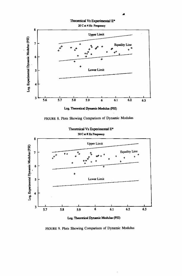
The laboratory E* values were compared against the theoretical values in plots shown in Figures 4 to 9. These plots show that the laboratory evaluated dynamic modulus agrees with the theoretical value for the same bituminous cures within a factor of two. This result is in agreement with other research findings that used other test methods in the laboratory. This result indicates to us that within a factor of two (of the actual value), the E* of bituminous concrete could be determined using theoretical methods if the basic properties of the mixture are known. This becomes very important especially when the E* is needed but could not be determined in the laboratory due to equipment or other problems. The theoretical E* then becomes a useful estimate of actual E* in situations like pavement design, overlay design, and statistical analysis for perfonnance prediction purposes.

CONCLUSION

Evaluation of the dynamic creep modulus, E*, of bituminous concrete has in the past been carried out by conducting rigorous laboratory tests. The E* of bituminous cores from the field were detennined using a direct

27

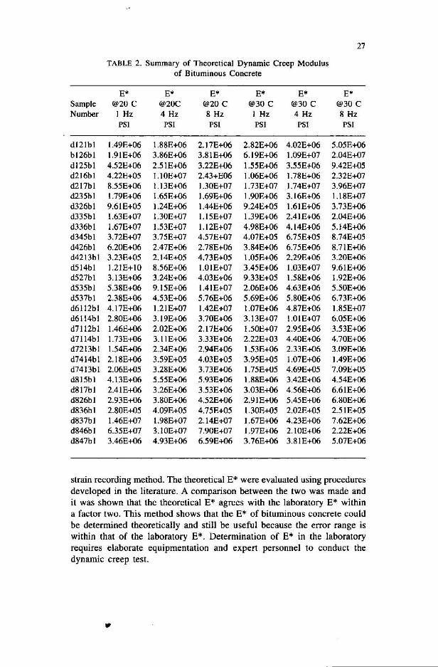
TABLE 2. Summary of Theoretical Dynamic Creep Modulus of Bituminous Concrete

E* E* E* E* E* E* Sample @20 C @2OC @20C @3OC @30 C @3OC Number I Hz 4 Hz 8 Hz I Hz 4 Hz 8 Hz

PSI PSI PSI PSI PSI PSI

dl21bl 1.49E+06 1.88E+06 2.17E+06 2.82E+06 4.02E+06 S.OSE+06 bl26bl 1.91E+06 3.86E+06 3.8IE+06 6.19E+06 I.09E+07 2.04E+07 dl2Sbi 4.52E+06 2.5IE+06 3.22E+06 I.5SE+06 3.SSE+06 9.42E+OS d216bl 4.22E+OS 1.l0E+07 2.43+E06 I.06E+06 1.78E+06 2.32E+07 d217bl 8.5SE+06 1.13E+06 I.30E+07 1.73E+07 1.74E+07 3.96E+07 d23Sbi 1.79E+06 1.6SE+06 1.69E+06 1.90E+06 3.16E+06 1.18E+07 d326bl 9.6IE+OS 1.24E+06 1.44E+06 9.24E+OS 1.6 I E+06 3.73E+06 d33Sbi 1.63E+07 1.30E+07 l.lSE+07 1.39E+06 2.4 I E+06 2.04E+06 d336bl 1.67E+07 I.S3E+07 1.12E+07 4.98E+06 4.14E+06 S.14E+06 d34Sbi 3.72E+07 3.7SE+07 4.57E+07 4.07E+OS 6.7SE+OS 8.74E+OS d426bl 6.20E+06 2.47E+06 2.78E+06 3.84E+06 6.7SE+06 8.71E+06 d4213bl 3.23E+OS 2.14E+OS 4.73E+OS I.OSE+06 2.29E+06 3.20E+06 dSI4bl 1.21E+1O 8.S6E+06 1.01E+07 3.4SE+06 1.03E+07 9.6IE+06 d527bl 3.13E+06 3.24E+06 4.03E+06 9.33E+OS I.58E+06 1.92E+06 dS3Sbi S.38E+06 9.ISE+06 1.41E+07 2.06E+06 4.63E+06 S.50E+06 dS37bl 2.38E+06 4.S3E+06 S.76E+06 S.69E+06 S.80E+06 6.73E+06 d6112bl 4.17E+06 1.2 I E+07 1.42E+07 1.07E+06 4.87E+06 1.8SE+07 d6114bl 2.80E+06 3.19E+06 3.70E+06 3.13E+07 1.0 I E+07 6.0SE+06 d7112bl 1.46E+06 2.02E+06 2.17E+06 I.SOE+07 2.9SE+06 3.53E+06 d7114bl 1.73E+06 3.IIE+06 3.33E+06 2.22E+03 4.40E+06 4.70E+06 d7213bl 1.54E+06 2.34E+06 2.94E+06 1.53E+06 2.33E+06 3.09E+06 d7414bl 2.18E+06 3.59E+OS 4.03E+OS 3.9SE+OS 1.07E+06 1.49E+06 d7413bl 2.06E+OS 3.28E+06 3.73E+06 I.7SE+OS 4.69E+OS 7.09E+OS d81Sbi 4.13E+06 S.5SE+06 S.93E+06 1.88E+06 3.42E+06 4.S4E+06 d817bl 2.4IE+06 3.26E+06 3.S3E+06 3.03E+06 4.56E+06 6.6IE+06 d826bl 2.93E+06 3.80E+06 4.52E+06 2.9 I E+06 S.4SE+06 6.80E+06 d836bl 2.80E+OS 4.09E+OS 4.7SE+OS 1.30E+OS 2.02E+OS 2.SIE+OS d837bl 1.46E+07 1.98E+07 2.14E+07 1.67E+06 4.23E+06 7.62E+06 d846bl 6.3SE+07 3.IOE+07 7.90E+07 1.97E+06 2.IOE+06 2.22E+06 d847bl 3.46E+06 4.93E+06 6.59E+06 3.76E+06 3.8IE+06 S.07E+06

strain recording method. The theoretical E* were evaluated using procedures developed in the literature. A comparison between the two was made and it was shown that the theoretical E* agrees with the laboratory E* within a factor two. This method shows that the E* of bituminous concrete could be determined theoretically and still be useful because the error range is within that of the laboratory E*. Determination of E* in the laboratory requires elaborate equipmentation and expert personnel to conduct the dynamic creep test.

..

• Theoretical Vs. E<perimental E·

2O.C. II HI PreqlJenC)'

9

iil e,. 8

Upper Limit !

i ::E

1 7 + • Equality

• +. Une + • t ++ + +

'3 +

.~ 6

! lower Limit

$ .. oS

4 6 6.1 6.2 6.3 6.' 6.5

Log. Theoretical Dynamic Modulus (PSI)

HGURE 4. Plots Showing Comparison of Dynamic Modulus

Theoretical V s E<perimental E· 30C.IHz~

8

Upper Limit til e,. 7

! + .. Equality Line + of' + + + + .+ + + +

6 + ... + + + .~ • ~

. +

S + +

+ '3 5 • Lower Limil

fi

1 w 4 OJ .. oS

3 5.6 5.7 5.8 5.9 6 6.1 6.2

Log. Th""Clicll Dynamic Modulu. (PSI)

F1GURE 5. Plots Showing Comparison of DynamiC Modulus

Theoretical Vs. Experimental E' 20 C. 1 Hz Fn=quency

10

~ 9

S 8

~ UppecUmit

" 7 Equality Line .~ .. +. • .. ,+, • , .. .. g. .... .. .. ...

6

"3 • .' .. Lower Limit

5 5

1 4 " '" ..

oS 3

2 5.8 5.9 6 6 .1 6.2 6.3 6.4

Loa. n-.tical Dynornlc Modulu. (PSI)

HGUl{c b. Ph.Jb ~hlJwil1g Comparison of Dynamic Modulus

~ticalVsExpcrimen~IE' 30 C M. 4 Hz Frequency

9

~ e:, ! 8 Upper Limil

I " 7 .~ Equality

g. " Line + + .. .. +, .. .. + .. t

i + 6 • ..

1 #" +

.:l 5 Lower Limit ..

oS

4 5.9 6 6.1 6.2 6.3 6.4 6.5

Log. Theoretical Dynamic Modulus (PSn

FIGURE 7. Plots Showing Comparison of Dynamic Modulus

...

• 1lIeoIWcal Vs Experimemal E*

20 C at 4 Hz Fmquc:ncy 8

Upper Limit

~ 7

i • Equolily Un.

++ • .. ." -/+ • " .+ • • +++ + .. ••

+ • . ~ 6 .. ! +

+

... "3 5

1 5 Lowei' Limit

.:l 4 .. .s 3

5.6 5.7 5.8 5.9 6 6.1 6.2 6.3

Log. n-<bcall>ynomic ModuIuI (PSI)

FIGURE 8. Plots Showing Comparison of Dynamic Modulus

Theoretical Vs Experimenlal E*

3OC .. IIh"'-Y

8

~ Upper Limit

;; e,

7 Equality Line !I •• + .. ~

~ .to "' .. • • ~

... • .. • • •• • • .. • • .w 6

l' • ...

"3 5 Lower Limit 5

1 .:l 4 .. .s

3 5.7 5.8 5.9 6 6.1 6.2 6.3

Log. Tbeoreti<all>ynlmic Modulus (PSI)

FIGURE 9. Plots Showing Comparison of Dynamic Modulus

PI

S ..... Sit' Sy' Sz V, Vb

NOTATION

Stiffness of Binder Temperature of Ring and Ball Test Penetration Value of Bitumen at 25"C Notation for the word Residual Notation for the word Initial Penetration Index Stiffness of Binder Parameters Percent of Aggregate by Volume Percent of Asphalt by Volume

REFERENCES

31

1. Goetz. W. H. The Evolution of Asphalt Concrete Mix Design Asphalt Concrete Mix Design: Development of a More Rational Approaches. ASTM STP 1041. W. L. Gartner, Ed., American Society for Testing and Materials. Philadelphia, 1985.

2. Von Quintas, H. L.. J. A. Scherocman, C. S. Hughes. and T. W. Kennedy. NCHRP Report No. 338, Asphalt-Aggregate Mixture Analysis System (AAMAS), Transportation Research Board, National Research Council, Washington, D.C., 1991.

3. Bonnaure, F., G. Gest., A. Gravais., and P. Uge. A New Method of Predicting Asphalt Paving Mixtures. Proceedings. Association of Asphalt Paving Technologists, 46, L 977.

4. Bolk, H.1.N.A .. The Creep Test, SCW Record 5, Netherlands, 1981. 5. Shell Pavement Design Manual. Shell Petroleum Company, London, 1978. 6. Yeager. L. L., and L. E. Wood. A Recommended Procedure for the Detennination

of the Dynamic Modulus of Asphalt Mixtures, JHRP-74-18, 1974. 7. Roberts F. L .. P. S. Kandhal , Dab-Yin Lee. and T. W. Kenedd)'. HoI Mi.

Asphalt Materials, Mixture Design. and Construction. NAPA Education Foundation. Lanham, Maryland. 1991.

8. Shakor R. Badaruddin. Prediction of Rutting in Bituminous Pavements From Field Sample Analysis. Journal. Institution of Engineers Malaysia, June, 1993.

9. Sousa, J. B., J. Craus, C. J. Monismith. Summary Repon on Permanent Deformation in Asphalt Concrete. SHRP, National Research Council. Washington D.C. , 1991.

to. Coree B. J. and T. D. White. The Synthesis of Mixture Parameters Applied to the Determination of AASHTO Layer CoeffLcient Distributions. Proceedings. Association of Asphalt Paving Technologists, 58, 1989.

11. Shakor R. Badaruddin. Development of Semi-Empirical Model to Predict Rutting in Bituminous Pavement. Inte rnational Journal of Science and Engineering, USA. [Accepted for Publication, Spring 1993).

12. C. van der Poel . A General System Describing the Viscoelastic Properties of Bitumen and its Relation to Routine Test Data. Journal of Applied Chemistry. 4. Pan 5, 1954.

13. Labtech Notebook Version 4. Manual. Data Acquisition Software. Laboratory Technology Corporation, Maryland, 1986.

Department of Civil and Structural Engineering Universili Kebangsaan Malaysia 43600 UKM Bangi Malaysia

...