© 2015 Kejia Chen

     

 

TRANSPORT OF SOFT MATERIALS IN CROWDED ENVIRONMENT

BY

KEJIA CHEN

DISSERTATION

Submitted in partial fulfillment of requirements for the degree of Doctor of Philosophy in Chemical Engineering

in the Graduate College of the University of Illinois at Urbana-Champaign, 2015

Urbana, Illinois

Doctoral Committee:

Professor Charles Schroeder, Chair Professor Steve Granick, Director of Research Professor L. B. Freund Professor Mary Kraft Professor Andrew Ferguson

ii  

ABSTRACT

Fluorescent microscopy was used to study the transport of soft material objects in

crowded environment. Delaunay triangulation and wavelet transform were adapted to extract

more information from images of macromolecules with irregular shapes and heterogeneous

transportation dynamics. Systems studied are actively transported endosomes in living cells, and

diffusing semi-flexible polymer chains in rigid networks. By going beyond traditional particle

tracking and trajectory analysis, it was discovered that for protein transportation rather than

directing the protein-containing endosomes steadily towards intended destination with regulatory

mechanisms as commonly believed, efficient random search is an alternative mechanism that can

offer both high energy efficiency and delivery accuracy. The imaging study of double-stranded

DNA molecules in actin and agarose gel showed that the popular mental image of a snake sliding

back and forth may not be how polymers actually reptate. The application of advanced analytical

tools to high resolution microscopy images of dynamic systems is expected to lead to the

discoveries of many more new mechanisms and concepts.

iii  

ACKNOWLEDGEMENTS

First of all, I want to thank my advisor, Prof. Steve Granick, for his constant

encouragement, patience, and support. He gave me full autonomy and showed me how to keep a

curious and open mind even after working on a problem for a long time. I would like to thank

Prof. L. B. Freund and Prof. Andrew Ferguson for taking interests in my research and providing

many thought-provoking ideas. I also want to thank Prof. Charles Schroeder and Prof. Mary

Kraft for sharing their expertise in DNA and membrane.

I would like to thank my lab mates at the Granick group. In particular, Dr. Bo Wang

started me on many interesting problems and showed me what it meant to be innovative and keep

a high standard. Dr. Juan Guan’s vivid descriptions were what first got me interested in the

research in this lab. Dr. Sung Chul Bae and Dr. Chang-Ki Min showed me the art of building

optical setups. Dr. Stephen M. Anthony introduced me to single particle tracking. James Kuo

taught me how to work with actin. Dr. Yan Yu answered my numerous questions about vesicles.

Changqian Yu showed me the way around the lab. Dr. Ah-Yong Jee helped me keep spirit high

after long strings of failed experiments. Boyce Tsang was always ready to explain to me complex

concepts in the most simple and clear manner. Adam Szmelter did much of the grind work on

some of the most challenging experiments presented in the dissertation.

Additionally, I want to thank Dr. George Bachand and Dr. Virginia Vandelinder at

Sandia National Lab, Marco Tjioe, Dr. Hannah Deberg, and Dr. Hyeongjun Kim from the Selvin

group, Sukrit Suksombat from the Chemla group, Nan Zheng from the Cheng group, Kieran

Normoyle from the Brieher group, Dr. Jeremiah Park from the Ha group, and Prof. Sang-Hee

iv  

Shim at UNIST. Their generosity in sharing their expertise and time has made research so much

easier and more pleasurable.

This work was supported by the U.S. Department of Energy, Division of Materials

Science, under Award No. DEFG02-02ER46019.

v  

TABLE OF CONTENTS

Chapter 1: Introduction…………………………………………………………..………………...1

Chapter 2: Diagnosing Heterogeneous Dynamics in Trajectories with Multiscale Wavelet............6

Chapter 3: Extending Particle Tracking Capability with Delaunay Triangulation….....................38

Chapter 4: Memoryless Self-reinforcing Directionality in Active Transport within Cells.............60

Chapter 5: Intermittent motion of semi-flexible polymers in network...........................................84

1  

CHAPTER 1

INTRODUCTION

1.1 Objective

While the transport of small molecules is well understood for a long time, the

mechanisms of transport of macromolecules, such as proteins and polymers, in crowded

environment are still being debated.1 There are many promising theories,2, 3 but the validation of

these theories has depended mostly on ensemble averaged scaling behaviors.4 Competing

theories can predict similar scaling at experimentally accessible time and length scales. These

experimental results therefore cannot conclusively prove or disprove different mechanisms.

The advancement of fluorescent microscopy has made it possible to image individual

macromolecules in crowded environment.5-8 We now have front row seats in watching these

macromolecules as they navigate their environment. This eliminates the need to deduce

individual behaviors from macroscopic observables. As the next step, we need to develop new

analytical tools to extract quantitative information from these unprecedentedly detailed images to

develop mechanistic understandings.9, 10

To go beyond traditional center-of-mass and second order moments based single-particle

tracking and trajectory analysis,11 methods developed in the graph theory and signal processing

fields were adapted to capture conformational information and to separate heterogeneous

dynamics. These new tools have led to the realization that unlike the transport of small molecules,

there are often multiple transport mechanisms that coexist and alternate intermittently. These

2  

tools have also revealed how different parts of a macromolecule, often exposed to different

environment, coordinate their motion.

This dissertation developed and applied two new analytical tools in the study of active

transport of proteins inside cells and DNA passive diffusion in actin and agarose gel networks.

1.2 Organization

In the following chapters, the developed analytical tools were first introduced in Chapter

2 and 3. These tools were then applied in two specific systems in Chapter 4 and 5.

Chapter 2: Based on wavelet transform, the method transforms raw data to

locally match dynamics of interest and thereby extracts and quantifies transient

heterogeneous dynamical changes from large datasets generated in single

molecule/particle tracking experiments. In separating the different dynamics, statistically

adaptive universal thresholding was used to avoid a single arbitrary threshold that might

conceal individual variability across populations. How to implement this multiscale

method is described, focusing on local confined diffusion separated by transient transport

periods or hopping events, with 3 specific examples: in cell biology, biotechnology, and

glassy colloid dynamics. The discussion is then generalized within the framework of

continuous time random walk.

Chapter 3: Delaunay triangulation is adapted to extend the capabilities of particle

tracking in three areas: (1) discriminating irregularly-shaped objects, which allows one to

track items other than point features; (2) combining time and space to better connect

3  

missing frames in trajectories; (3) identifying shape backbone. Specific examples were

given for each of the capabilities.

Chapter 4: A large set of trajectories of protein-containing endosomes in living

cells were analyzed using the above two methods. Brownian-like steps in endosome

transport were observed to self-organize into truncated Lévy walks through a positive

feedback in directional persistence. Lévy walks have functional advantages over

Brownian motion in random searching and transport kinetics and we believe Lévy

dynamics can be an efficient alternative to highly regulated transport. Although the

random nature of the transport has been reported before, the particular type of random

walk the motion follows is rather surprising. In classic random walk models, it is

common to introduce memory kernels to describe Lévy dynamic, the required memory

over long time and large length scales lacks obvious reasonable grounding here. A

molecular model was developed that shows the slow fluctuations of the number of

available motors, coupled nonlinearly to the fast motor binding and unbinding events

through the load-dependent unbinding rate is sufficient to produce the effective positive

feedback that constructs Lévy dynamics from Brownian steps.

Chapter 5: Images of fluorescently labeled λ-DNA chains threaded through F-

actin or agarose network meshes were analyzed using the methods described in Chapter 2

and 3. A strong coupling between shape fluctuation and chain transport was identified.

The shape and motion of a chain are simultaneously arrested most of the time and

spontaneous large shape fluctuation transiently allows a chain to break free and achieve

4  

net transport. This was observed at both individual chain and ensemble level. Tracking

the chain ends reveals that the end motion is also intermittent, which can lead to the arrest

of shape and chain motion. The duration of the arrested phase suggests a heterogeneous

transport barrier. This novel mode of transport might be important to transport in porous

media and crowded environment as shape fluctuation is widely present in a broad class of

soft materials.

1.3 Future Prospects

While the analytical tools developed here have some generality, many more new tools are

expected as the imaging subjects diversify. Although these new tools will extract ever more

information, there is the danger of over-interpretation. The complexity of these new analyses and

lack of a universal approach also mean it will be harder for readers to fully appreciate these

results and therefore to advance the field. Accompanying mathematical equations with the

physical meaning in each application is therefore very important; while careful control analyses

and verification with multiple approaches will help prevent over-interpretation of the microscopy

images.

1.4 References

1. Fakhri, N., MacKintosh, F.C., Lounis, B., Cognet, L. & Pasquali, M. Brownian motion of stiff

filaments in a crowded environment. Science 330, 1804-1807 (2010).

2. Aradian, A., Raphael, E. & de Gennes, P.G. A scaling theory of the competition between

interdiffusion and cross-linking at polymer interfaces. Macromolecules 35, 4036-4043 (2002).

3. Muthukumar, M. Mechanism of DNA transport through pores. Annual Review of Biophysics and

Biomolecular Structure 36, 435-450 (2007).

5  

4. Everaers, R. et al. Rheology and microscopic topology of entangled polymeric liquids. Science

303, 823-826 (2004).

5. Guan, J., Wang, B., Bae, S.C. & Granick, S. Modular stitching to image single-molecule DNA

transport. Journal of the American Chemical Society 135, 6006-6009 (2013).

6. Tokunaga, M., Imamoto, N. & Sakata-Sogawa, K. Highly inclined thin illumination enables clear

single-molecule imaging in cells. Nature Methods 5, 159-161 (2008).

7. Teixeira, R.E., Dambal, A.K., Richter, D.H., Shaqfeh, E. & Chu, S. The individualistic dynamics

of entangled DNA in solution. Macromolecules 40, 2461-2476 (2007).

8. Robertson, R.M. & Smith, D.E. Direct measurement of the intermolecular forces confining a

single molecule in an entangled polymer solution. Physs Revs Letts 99 (2007).

9. Valentine, M.T. et al. Investigating the microenvironments of inhomogeneous soft materials with

multiple particle tracking. Physical Review E 64 (2001).

10. Granick, S. et al. Single-molecule methods in polymer science. Journal of Polymer Science Part

B-Polymer Physics 48, 2542-2543 (2010).

11. Crocker, J.C. & Grier, D.G. Methods of digital video microscopy for colloidal studies. Journal of

Colloid and Interface Science 179, 298-310 (1996).

6  

CHAPTER 2

DIAGNOSING HETEROGENEOUS DYNAMICS IN

TRAJECTORIES WITH MULTISCALE WAVELET

2.1 Background

The experimental study of dynamics has been deeply transformed during the past

generation by new technologies that acquire digital images in vast quantities, allowing one to

record motion of objects of interest, one-by-one in real space and time.1-7 When datasets of this

kind are analyzed, the capacity to track individual objects over a long time allows not only

quantification of individual variations within populations but also complex temporal fluctuations

of individual moving elements. The valuable information offered by huge datasets goes beyond

what can be obtained from the classic ensemble-averaged approach, and has often provided

unexpected mechanistic insights. This approach of “deep” statistical imaging has already led to

significant progress in a variety of fields, from physical sciences such as diffusion6-11 and other

dynamics in condensed matter,5, 12, 13 to biological sciences such as ecology14 and cell biology.15-

17 Much important work revolves around improving experimental techniques to collect the

data.18, 19

                                                              Adapted with permission from Bo Wang, Juan Guan, and Steve Granick (2013) Diagnosing

Heterogeneous Dynamics in Single Molecule/Particle Trajectories with Multiscale Wavelets, ACS Nano,

7, 8634-8644. Copyright 2013 American Chemical Society

 

7  

Here we ask a different question: how to analyze such data for embedded information?

For many problems, but not all, it is reasonable to assume random fluctuations with some

probabilistic distribution around an average value. However, dynamics in the physical and

biological worlds are often heterogeneous. When the statistical character of the process changes

intermittently with time due to stochastic switching between coexisting and often competing

microscopic processes,1-17 averaging over these distinct processes may give misleading results.

Progress is impeded by the paucity of methods to identify these distinct processes, and to

quantify them, especially in the presence of noise in the data. An ideal method would be

automated to handle large datasets, involve no judgment on the part of the analyst, and resolve

rapid dynamic changes. In practice, to differentiate different modes of motion, one selects a

metric of interest. Some of the metrics commonly used with aggregates of data include the

scaling of mean square displacement (MSD),20-22 correlation functions,23, 24 diffusion

coefficient,25 and other trajectory characteristics.26-28 While each of these performs well for

certain particular systems, these families of methods require prior information or assumptions

about the character of the motion.

A delicate matter is to select the appropriate time window over which to seek dynamic

changes of the observables. Too short a time can exaggerate noise but too long sacrifices

temporal resolution and increases the chances of undesired mixing of distinct processes that

switch more rapidly. Further, one needs to accumulate reliable statistics, but rare and transient

events are too-readily averaged out, especially as reliability typically requires at least hundreds

of data points. Also problematical is to select a criterion by which to distinguish random

fluctuations from real changes in dynamics; there is no general way to avoid judgment in

selecting these thresholds, and judgment risks being arbitrary, too subjective, and too demanding

8  

of different definitions depending on the case at hand. Taking a different approach, probability

inference can be used to choose between models, maximizing the likelihood that a certain model

fits the data.22, 25, 29 But this presents its own complexity, especially because it requires prior

assumptions in associating the data to particular models.

This chapter presents wavelet transforms and universal thresholding as useful techniques.

Developed in the field of digital signal processing,30-33 here we show how to apply wavelet

analysis to detect dynamic changes hidden in time-resolved positional trajectories of physical

and biological systems. The advantage of this method is that it analyzes data on multiple scales

simultaneously by decomposing time series into a full set of time scales while preserving

information in time and frequency domains simultaneously. The following discussion presents

first the method, then demonstrates its usefulness in three dynamical physical systems involving

soft and biological matter, and concludes by generalizing the discussion.

2.2 Results and Discussions

2.2.1 Methodology

The qualitative principle of wavelet analysis is simple:30-32 moving along a time series of

observables, transient changes in dynamics result in wavelet coefficients with large absolute

values, as wavelet transform is known to be very effective at detecting discontinuity. Fig. 2.1a

shows schematically the main idea: a time series of raw data is expanded to time-resolved

wavelet coefficients on different scales (or frequency), by convolution over local times with the

wavelet basis function. Background “noise”, which represents in part random fluctuations, in

part the mixing of different processes in the system, is measured on small scales (high

frequency), and projected statistically to larger scales (low frequency) generating a “universal

9  

Figure 2.1. The main idea of wavelet analysis implemented in this study. (a) Schematically: the

information embedded at small and large scales in a time series of raw data is expanded by

wavelet transform. The information at small scale provides a global estimate of “noise” level and

generates a universal threshold that can be projected onto long times, allowing one to localize

“signal” from noisy background. (b) Spatial position plotted against time in an illustrative

trajectory. (c) The corresponding wavelet coefficients are plotted against time as the result of

local integration using the Haar continuous time wavelet transform (CWT). Red: positive values;

blue: negative, green and yellow: near-zero. Dynamics of interest are identified on the scale

(frequency) over which bands of coefficients are distinct. Information is lost if the scale is too

large (frequency too small), whilst noise overwhelms events if the scale is too small (frequency

too high). The usable range of scales is in between two black lines. Arrows in panel (b) point to

two events of interest for further analysis. A time span of background noise is also highlighted in

(b).

10  

threshold” that naturally adapts to the noise amplitude. This threshold allows one to discriminate

dynamics of interest, “signal” that exceeds this threshold, on larger scales.

One inspects a time series of an observable (Fig. 2.1b). There results a spectrum of

wavelet coefficients against time and scales (Fig. 2.1c). Over small scales, the wavelet

coefficients are dominated by featureless random fluctuations, whereas at large scales, the

coefficients of given time points are heavily distorted by dynamics extending for long times

around it. Importantly, at the intermediate scales, transient changes above background

correspond to distinct bands in wavelet coefficients that can be resolved with confidence.

Detecting the convergence to these local maxima of wavelet coefficients on these scales localizes

dynamic heterogeneity, the information we seek. As explained below, this local detection has a

time resolution better than the exact scale on which this analysis is carried out. This statistically

rigorous multi-scale method overcomes the current difficulties in analyzing heterogeneous

dynamic data as we have introduced.

To implement the method there are 4 steps: (a) choose the wavelet basis function; (b)

perform the wavelet transform; (c) determine the scale and threshold; (d) assign the physical

processes.

Wavelet selection.

The wavelet transform calculates the local integral values of time series over various

scales with weighting defined by the wavelet function used. Different scales generate a times

series of wavelet transform coefficients corresponding to different time scales. Specifically, the

11  

wavelet transform30-32 of a time series s t on scale a is

00

1,

t tC t a s t dt

a a (1)

where the wavelet function has width a , centered at time 0t . To satisfy Lipschitz continuity,

local maxima of 0 ,C t a correspond to singularities in s t . Therefore, to detect dynamical

changes, one searches for regions converging to local maxima in 0 ,C t a along 0t .

The appropriate wavelet depends on the nature of the dynamic heterogeneity for which

one searches. Ideally, to choose an efficient wavelet, one needs to maximize the cross-correlation

between wavelet and the signal of interest, as it would produce highest local maxima in wavelet

domain and thus improve the localization of the signal. This can be achieved by screening

through known wavelet libraries: Daubechies, Symmlets, Coiflets, and many others.31 However,

we emphasize that the choice of wavelet must be physically driven. For example, if the

background contains fluctuations around an average level but the signal shifts the average, then

one selects with one vanishing moment (such as Haar wavelet), also known as Daubechies 2

wavelet, such that local maxima in 0 ,C t a correspond to discontinuity above this constant fast

fluctuating component. This situation includes all three examples discussed below, as well as

single molecule FRET time traces that have been reported earlier.34, 35 As another example, when

the dynamics exhibits abrupt, fast back-and-forth jumps between several positions/states (e.g.

harmonic oscillators in double potential wells), the detection should target maximum curvature

in the trajectory. Then one selects with two vanishing moments (such as Daubechies 4

wavelets) such that local maxima in 0 ,C t a correspond to maximum curvature in trajectories.30

Similarly, when targeting discontinuity in gradients, Daubechies 6 wavelets with three vanishing

12  

moment should be used.30 While the mathematical steps of implanting this method are

straightforward, as a premise one needs judicious judgment of what type of motion to target.

In the three physical examples discussed in detail below: we choose the wavelet on a

physical basis. These are the cases of local confined diffusion separated by transient transport

periods or hopping events so the appropriate wavelet should have one vanishing moment. In

particular, “Haar wavelet” quantifies the displacement between the average position of n points

before and after position i along a trajectory with equal weighting to the position of all the points

around the center point:

1( , 2 )

i n i n

j jj i j i

C i n x xn

. (2)

What this means physically is quantifying the drift of mean position over time. For

Brownian motion, there is no drift of the mean position, which wanders around zero, but for

directional transport, drift is decidedly finite. The point may seem paradoxical, as everyone who

has tossed coins is familiar with the fact that the numbers of heads and tails are rarely equal, due

to statistical fluctuations. It is a matter of scale: as the time scale increases, the difference

between the mean positions becomes pronounced. The wavelet transform must be evaluated over

scales that are long enough.

Implementing the wavelet transform.

The wavelet is mathematically defined as local integrals according to Eq. (1), but in

practice it is more efficient computationally to compute the coefficients by correlations between

a short section of the time series data and the chosen wavelet, shifting and stretching the wavelet

according to 0t and scale a . Using MATLAB for convenience, we compute continuous wavelet

13  

coefficients at real, positive scales of trajectories projected onto x and y dimensions separately.

An example is shown in Fig. 2.1. This shows the result of a trajectory transformed into time

series of coefficients over various scales.

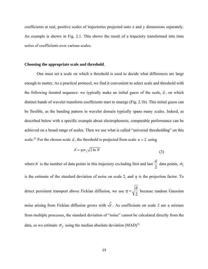
Choosing the appropriate scale and threshold.

One must set a scale on which a threshold is used to decide what differences are large

enough to matter. As a practical protocol, we find it convenient to select scale and threshold with

the following iterated sequence: we typically make an initial guess of the scale, a , on which

distinct bands of wavelet transform coefficients start to emerge (Fig. 2.1b). This initial guess can

be flexible, as the banding pattern in wavelet domain typically spans many scales. Indeed, as

described below with a specific example about electrophoresis, comparable performance can be

achieved on a broad range of scales. Then we use what is called “universal thresholding” on this

scale.31 For the chosen scale a , the threshold is projected from scale 2a using

2 2 ln N (3)

where N is the number of data points in this trajectory excluding first and last 2

a data points, 2

is the estimate of the standard deviation of noise on scale 2, and is the projection factor. To

detect persistent transport above Fickian diffusion, we use 2

a

because random Gaussian

noise arising from Fickian diffusion grows with t . As coefficients on scale 2 are a mixture

from multiple processes, the standard deviation of “noise” cannot be calculated directly from the

data, so we estimate 2 using the median absolute deviation (MAD)31

14  

2

median ( ,2)

0.6745i C i

(4)

Finally, we refine the scale and threshold through iterated assignment and validation of

training trajectories, if necessary. Criteria by which to decide whether refinement is needed are

(a) whether the assignments are insensitive to small changes of scale and threshold, and (b)

whether other metrics, such as MSD and correlations, are separated in ways that are anticipated

based on physical characters of these processes.

Note that while this detection method is local, the estimate of noise level is global, as the

entire trajectory is used to estimate the noise level. This gives reliable and fully automatic

thresholding adaptive to each individual trajectory, with thresholds reflecting the heterogeneity

between trajectories. Although this “universal threshold” assumes a Gaussian noise, in

implementing this method, we have noticed empirically that regardless of the exact statistical

characteristics of noise, a wide range of scales give equally robust separation, as will be

illustrated below. Physically, the reason is that the dynamics of interests are so well separated

that the details do not make a decisive difference.

Interpreting data to assign physical process.

Naturally, the physical process of interest depends on the problem at hand. In the sections

below, we present three examples of distinguishing between “signal” and “noise.” In all three

examples the “signal” contains heterogeneity that is characteristic of the system, and the noise

describes the Brownian component that constantly fluctuates as background.

Assignment proceeds by combining the time periods during which wavelet coefficients

on scale a exceed the threshold . For multidimensional trajectories, e.g. x, y, and z in

Cartesian space, this is repeated for each dimension and the results are combined. When the

15  

trajectories are isotropic, a common threshold can be used for all dimensions. When dimensions

are statistically dependent, separate thresholds should be used for each dimension. The

confidence of assignment depends on the trajectory length, especially for very short trajectories,

as then a reliable estimate of noise level becomes impossible. We typically discard trajectories

shorter than 300 data points.

2.2.2 Three Examples

To test the efficacy of this method and to illustrate the operation in practice, we illustrate

this wavelet analysis with three examples: to distinguish active transport from passive diffusion

of single-particle motion in cell biology, to identify pauses of single-molecule DNA trajectories

in electrophoretic mobility, and to capture intermittency of single-particle glassy dynamics.

Focusing on the first example, the latter two examples illustrate that this method is general.

Active transport in living cells.

Intracellular transport of endosome “cargo” proceeds by a stochastic switching between

passive diffusion and active transport along microtubules, dragged by motor proteins, kinesin

and dynein.36 This switching between two types of motions, active and passive, is known to

happen on sub-second time scales; in function, it enhances cell reaction kinetics and maintains

cellular functions.37 It is of fundamental significance to resolve active processes uncontaminated

by passive fluctuations, but to do so, methods are needed to discriminate between them.

The data are contained in a Ph.D. thesis.38 Using fluorescence microscopy (see experimental

details below), we obtained trajectories of EGF-containing endosomes in living HeLa cells and

we implemented wavelet analysis to assign passive and active motion. From raw data of

16  

trajectories illustrated in Fig. 2.2a and Fig. 2.2b, two types of motions cannot be distinguished on

short time scales. We computed the Haar wavelet coefficients at a scale of 32 frames for all

trajectories (Fig. 2.2c), a scale on which banding of wavelet transform coefficients is clearly

distinguishable. The threshold was set according to universal thresholding with results indicated

in gray in Fig. 2.2c; the segments that exceed the threshold were assigned as active. Combining

results both on x, and y, the separation is overlaid on the original trajectory in Fig. 2.2a, with

active portion highlighted in red. Fig. 2.2d shows that the assigned active segments were

invariably super-diffusive while passive segments were invariably either diffusive or sub-

diffusive, which is reasonable physically.

The major advantage of wavelet analysis, for this example, is considered to be that

universal thresholding is adaptive to heterogeneities between trajectories. We found the imputed

thresholds to vary by two orders of magnitude, depending on the noise level, quantified by

frame-to-frame displacement (∆r) of that particular trajectory (Fig. 2.3a). We conclude that

universal thresholding is adaptive. Nonetheless, Fig. 2.3b shows that according to the trajectory,

the imputed active fraction spanned a wide range that was independent of the threshold,

suggesting that thresholding did not introduce an artificial bias such as low thresholds giving

large active fraction or vice versa. The arrows point out trajectories, which are <10% of all, for

which after the initial assignment, fine-tuning of the threshold was necessary. They were the

trajectories that are statistically biased with a prohibitively large fraction of active transport to

estimate the passive fluctuations using MAD (Eq. 4). They were identified during the refinement

step where for each individual trajectory, the mean square displacement (MSD) of the assigned

passive portion was calculated and fit as a power law in time, 2r t , where 1 is

17  

Figure 2.2. Example: a cell biology problem involving single-particle imaging of endosome

transport along microtubules by molecular motors. (a) From a plot of the trajectory, x against y

in Cartesian coordinates, wavelet analysis identifies active (red) and passive (gray) segments of

the trajectory. (b) During this trajectory acquired by time-lapse imaging, the frame-to-frame

displacement in the x direction (20 fps) is plotted against time. (c) The wavelet coefficients of

this data at scale 32 frames are plotted against time, indicating the middle band of small

coefficients that we identify with passive diffusion and the extreme values of wavelet

coefficients that we identify with active motion. (d) Mean square displacement (MSD) is plotted

against time on log-log scales for “active” (red) and “passive” (gray) segments of this trajectory.

The shaded gray region demarcates the lower limit of Fickian diffusion with log-log slope 1, and

upper limit of directional motion with log-log slope 2. These trajectories imputed from wavelet

analysis split into two families, sub-diffusive (passive) and super-diffusive (active).

18  

expected for passive motion according to physical reasoning. For these trajectories, the fitted

initially exceeded 1.1, and the thresholds were decreased and the process repeated iteratively

until the criterion 1.1 was satisfied. This refinement is a technical compromise for a small

portion of the data that is imperfect; it is not an intrinsic problem of the method. This process is

optional. While we chose to lower the threshold to rescue the data as much as possible,

alternatively, these biased trajectories can be excluded from the downstream analysis.

Figure 2.3. The universal threshold is adaptive and unbiased. Continuing the cell biology

example, for this scatter plot of 3443 endosome transport trajectories, each trajectory’s threshold

is determined individually and plotted against (a) average frame-to-frame displacement (∆r) and

(b) imputed active fraction of that trajectory. The black lines are drawn to guide the eye,

indicating the thresholds on noise level but not the active portion of individual trajectories.

Arrows note a subpopulation of trajectories (<10% of the total), for which universal thresholding

needs refinement. The reasons for refinement are described in the text, and the text describes

how to fine-tune the threshold iteratively and automatically.

 

19  

Figure 2.4. The choice of wavelet function depends on the physical problem. Continuing the

cell biology example, a zone where the trajectory traces out loops corresponds to the boxed area

in Fig. 2.2a. (a) Implementing the Haar wavelet, we assign a large portion of the loops (indicated

by the arrows) as passive (gray), whereas (b) implementing the Daubechies 4 wavelet we assign

them as active (red), but these two wavelets make the same identification elsewhere in the

trajectory. The Haar wavelet is nonetheless preferred except for special circumstances owing to

its simple, physical interpretation as a drift of mean position.

 

To test the accuracy of the assignment, we disrupted microtubules using nocodazole,

which eliminates active transport, and then the trajectories were analyzed as before. Fewer than

0.1% of total steps were mistakenly assigned as active motion. To further test the reliability of

the wavelet-based assignments, manual checks were performed. We inspected 10 representative

trajectories, a total of 16,816 image frames, and manually assigned the active frames. This visual

inspection found that false-positives of active steps amounted to only ~5% of the total active

steps. Also, visual inspection suggested that ~20% of the active steps were missed by the wavelet

analysis. Similar performance was confirmed on simulated trajectories (Methods Section). As

visual inspection was subjective, we are unable to decide to which method more confidence

should be given. Our main conclusion is two-fold. First, errors of the wavelet analysis tended to

20  

err on the conservative side, tending to mistakenly assign active steps as passive motion.

Detailed arguments concluded that these miss-assignments did not bias the data.38 Second, this

conservatism resulted in excellent discrimination of the active steps themselves.

The visual inspection suggested that miss-assignments occurred at the transition of active

and passive motion. Other false negatives identified manually are more debatable. For example,

sometimes the active motion circled around or reversed directions as shown in Fig. 2.4.

Depending on the dynamics of interest, one may or may not want to identify these motions. The

Haar wavelet (Daubechies 2) will assign them as passive (highlighted by arrows in Fig. 2.4a) as

the drift of mean position approaches zero at those points; while wavelet with 2 vanishing

moments (here we use Daubechies 4 for simplicity), which targets motions that introduce abrupt

changes in local curvature, will assign them as active (Fig. 2.4b). So an appropriate wavelet

should be selected based on the need.

Advantages of this analysis are considered to be mainly two. First, large datasets were

processed automatically in a short time. Visual inspection would have been prohibitive; the

visual inspection of 10 trajectories just mentioned consumed roughly 5 hr, whereas on a PC 3443

trajectories were analyzed in 10 minutes. Second, the wavelet analysis suggested significantly

new conclusions about the physical process. Wavelet analysis identified that EGF-containing

endosomes in HeLa cells spend around 30% of the total time (879,427 out of 3,211,776 steps) in

active transport, which is consistent with the manual assignment of 27%. In contrast, the fraction

found by existing methods reported in the literature21, 23, 26 was less than 5% with more false

positives (see Methods Section for details). Furthermore, while subjective visual inspection

suggested that the average duration of continuous active transport is ~1.1 s, this number was

~0.75 s using wavelet analysis but less than half of this (~0.3 s) using the other methods.21, 23, 26

21  

Although visual inspection can be subjective and likely misses short active durations, these

simple but important measurements are considered to indicate that wavelet analysis presents a

significant improvement. This high-throughput analysis can provide statistics needed to compute

velocity autocorrelation functions, velocity distribution functions, as well as directional

persistence of active transport.

Intermittent mobility in DNA electrophoresis.

Recent single-molecule measurements from this laboratory show that when -DNA

migrates through agarose gel under the action of an electric field, the time-dependent position of

individual molecules proceeds in spurts with pauses in between.39 This is another problem of

how to separate “signal” (the spurts) from “noise” (the pauses), in the presence of uninteresting

background noise. While to the eye it may be obvious that molecular mobility exhibits two states

(Fig. 2.5a), to automatically separate these two is challenging, as the frame-to-frame

displacements of center of mass shows no temporal pattern above random fluctuations (Fig.

2.5b).

To discriminate these two mobility states, a wavelet analysis was used on each single-

molecule trajectory. On scales 8 and 32, the universal threshold separated the pauses and jumps

nicely for λ-DNA in 1.5 wt% agarose gel under electric field 12 and 6 V/cm respectively (Fig.

2.5a and c). At each field strength, a range of scales give good separation (Fig. 2.5c). Too-small

scales result in missing a large portion of spurts, too-large scales assign mistakenly many pauses

as spurts. The envelope of usable scales (which still spans a broad range) decreased with field

strength because, as the lifetime of pausing shortened as the force on the DNA molecules

increased, shorter scale became better at most accurately assigning these faster transitions.

22  

Figure 2.5. Example: a biotechnology problem involving single-molecule imaging of DNA

electrophoresis in agarose gel as described in the text. (a) Illustrative trajectories showing that

DNA center of mass motion at 12 V/cm is discontinuous, the wavelet analysis identifying spurts

of rapid motion (red) and pauses between spurts (gray), neither of them equal to the mean speed.

The trajectory at 6 V/cm drive is discontinuous likewise. (b) Frame-to-frame displacement of a

6V/cm trajectory (33 fps) is plotted against time. (c) This panel compares efficacy over a broad

range of scale of analysis as well as drive voltage. Over a broad intermediate range of scale the

mobility separation of this electrophoresis data is robust without depending on the specific

choice of scale. Symbols represent examined conditions: solid, successful separation, open: poor

separation.

23  

Analyzing ~1,000 trajectories we found that spurts comprised 30% (68,222/230,057

steps) and ~60% (61,436/102,574 steps) of the total time elapsed, under electric field 6 and 12

V/cm respectively. The speed during spurts much exceeded the mean speed (Fig. 2.5a). This

significant contrast would not have been quantified otherwise, and provides firm numbers from

which to examine competing electrophoresis theories.40

Hopping dynamics in a colloidal supercooled liquid.

It is well established that dynamics in supercooled liquids is intermittent.12, 41, 42 As

illustrated in Fig. 2.6a, in both positional and angular space, trajectories are at first restricted to a

narrow region of space, then hop suddenly to a new region, probably reflecting collective

rearrangements of the neighbors.42 Despite numerous previous studies, such hopping events are

hard to identify automatically in large datasets. The difficulty is that, during hopping,

displacements or directional persistence of the motion do not necessarily differ from those during

caging (Fig. 2.6b), and the duration of the hopping is typically short, if not instantaneous.

Therefore, these events are often characterized ambiguously as “fat tails” of total ensemble-

averaged displacement distributions.6, 12, 41

However, these abrupt changes present pronounced peaks in wavelet transform

coefficients (Fig. 2.6c). By the methods described above, they can be located precisely by a

wavelet analysis. Detecting hopping in this way, one notices hopping simultaneously in position

and rotation, indicating that rotational motion correlates closely with translational motion. This

observation agrees with our previous conclusion drawn from ensemble-averaged correlation

functions,42 but from the wavelet analysis the evidence of rotational-translational coupling is

made more direct.

24  

Figure 2.6. Example: a glassy dynamics problem involving the identification of hopping events.

(a) Typical raw data showing an angular trajectory, plotted against (these are the out-of-

plane and in-plane angles respectively) and the concomitant positional trajectory, x plotted

against y, for the index-matched colloidal glass discussed in the text, showing the wavelet-

identified hops (red) between regions of caged motion (gray). (b) Plotted against time, one

observes the frame-to-frame in-plane angular and spatial displacement of these trajectories. (c)

Coefficients of the wavelet transformation of the time series, evaluated at scale of 16 frames, are

plotted against time for the in-plane angle and the y spatial position, each threshold denoted as a

horizontal dashed line. The vertical red bar shows the interval when wavelet coefficients exceed

the threshold, which identifies the hop. (d) Dependence of the imputed hopping time, which

defines the time resolution of the method, on the wavelet scale and threshold selected to analyze

it. The threshold from universal thresholding is adjusted down or up by a constant factor of 0.9

(red), 1.2 (green), and 1.5 (blue).

25  

Figure 2.7. Analysis of continuous time random walk (CTRW) simulated from known data,

showing how the analysis depends on various amounts of added noise type and noise level.

Noise level is measured in multiples of standard deviation of the signal, s . First, for different

types of noise, the dependence on noise amplitude is shown of the false positive rate (a) and false

negative rate (b): zero noise (red squares), single component Gaussian noise (green asterisks),

compounded Gaussian noise (magenta circles), time varying noise (blue triangles). Also, for

three thresholding methods, the dependence on noise amplitude is shown of the false positive

rate (c) and false negative rate (d) plotted against noise amplitude for three thresholding methods

and single component Gaussian noise: universal threshold (red squares), SURE (green asterisks),

and Minimax (blue circles).

 

As this transition is so sharp, and presumably instantaneous, this example poses a

stringent test for the time resolution of our method. Therefore, we used the hopping time as the

shortest duration of events that can be detected with wavelet analysis, and this defines the time

resolution of the method. Fig. 2.6d shows that the time resolution improves when the scale

26  

becomes smaller and the threshold increases. However, the difference is small, suggesting that

the time resolution is related to but is not limited by the scale on which the analysis was carried

out. As a rule of thumb, a wide range of scales gives similar time resolution, ~5 frames. Further,

by changing the time between evaluations of the data, we showed that the time resolution is

largely unaffected. These tests demonstrated the robustness of the method and the ability to

identify truly transient dynamics.

With this method, it would be interesting to revisit the enormous amount of data that is

available in the literature, 6, 12, 41 to directly measure the caging time, as well as its distributions,

when approaching the glass transition. Further, using these hopping events as reference points,

one could examine the dynamic paths and structural organizations around those events.

Information of this kind could be difficult to obtain otherwise, as rare events of this kind can be

buried deeply in conventional correlation functions that average over all time.

 

2.2.3 Generalization

The above three examples are variations of dynamic processes with rapid motions

(jumps) and waiting periods between them. Such dynamics can be described as continuous time

random walks (CTRW), widely reported in single particle tracking data.43, 44 To generalize this

discussion, we simulated standard one-dimensional CTRW trajectories with power-law

distributed waiting time between steps and exponentially distributed jump size (Fig. 2.7a),45 and

applied the wavelet analysis on these trajectories to identify the jumps. As by construct here we

have perfect knowledge of where the jumps are, it allows us to evaluate the method’s

performance more rigorously and explore how the performance is affected by experimental

27  

complications such as noise level and type. It also allows us to directly compare alternative

techniques to compute the thresholds.

First we confirmed that, in the ideal case where there is no noise, wavelet analysis

identifies the periods of motion almost without fault; in Fig. 2.7b and 7c the false positives rate is

0.43% and the false negative rates is 1.43%. Then, we considered complications in practice. In

experiments, multiple sources of noise often coexist, among them localization error and thermal

fluctuation.46 The noise magnitude often increases with time; for example, signal dims as dye

molecules bleach, which amplifies the localization error in tracking experiments. To evaluate

such potential pitfalls, we added increasing magnitudes of three simulated types of noise:

constant Gaussian noise, non-Gaussian noise with two components, and noise with increasing

amplitude with time (see Methods for details). No significant difference in outcome resulted

(Fig. 2.7b-c), demonstrating the robustness of the method. We also observed that even when the

noise level was so large that it was comparable to the signal itself, the false positive rate

remained small while even eyes would have a false positive rate close to 50%. Consistently, we

found more false negatives than false positives, as the universal threshold is known to be strict.

This “strictness” is desirable as false positives are more probable to introduce bias in

downstream analysis.

Now we compare other threshold computing techniques, such as SURE (Stein’s unbiased

estimate of risk) and Minimax.47 Similar performance was observed for the physical situations

considered in this chapter (Fig. 2.7d-e). This observation is reassuring, as the efficacy of

separation should not critically depend on how the wavelet analysis is implemented. Our purpose

is to set up a general platform. Of course, other thresholding techniques, known and well-

28  

developed in the field of digital signal processing, could alternatively be employed as appropriate

for other needed circumstances.

2.3 Conclusions

We have described a robust method to automatically detect dynamic heterogeneity in

time series data that are collected routinely in many labs across various fields. We have applied

this method to three separate examples: in cell biology, biotechnology, and soft matter physics,

to illustrate and validate the method, and to demonstrate its broad usefulness. Since the analysis

makes no assumptions about the physical nature of the dynamics, we emphasize that the method

is general. Selecting the wavelet, the scale, and the threshold are the three main steps of the

method, and our examples along with discussion show when and how the method’s performance

depends on the educated choices that the user makes about these prime considerations. We note

that, while these parameters need to be chosen on physically-motivated grounds, performance of

the method is robust within broad ranges of parameters, and insensitive to various experimental

complications.

It is impossible to achieve perfect separation without full knowledge of the microscopic

mechanism. One only can do so with a certain level of statistical confidence, depending on the

method used. Apart from the wavelet method described in this chapter, the existing methods fall

into two categories. One class is based on fitting the data to presumed models. A second class is

based on ensemble-averaged quantities which suffer from incompatibility between time

resolution and statistical reliability. With 3 applications discussed above, and in another test of

the method using simulated data whose statistical character was known precisely by direct input

of the data, we have discussed how a wavelet approach can aid in going beyond these limitations.

29  

2.4 Materials and Methods

Active transport.

Endosomes in HeLa cells were fluorescently labeled by incubating the cells with 0.15

µg/mL biotinylated EGF complexed to Alexa-555 streptavidin (Invitrogen) for 20 min. The

endosomes were tracked under physiological conditions on a homebuilt microscope in a highly

inclined illumination optical (HILO) geometry with the laser beam inclined and laminated as a

thin optical sheet with thickness of ~1 µm into the cells.48 To avoid focal plane drifting, the

objective was simultaneously heated and immersion oil with ultralow fluorescence standardized

at 37 °C (Cargille) was used. Fluorescence images were collected by a back-illuminated electron

multiplying charge-coupled device (EMCCD) camera (Andor iXon DV-897 BV). Typically,

each movie lasted 4,000 frames at a frame rate of 20 fps. The movies were converted into digital

format and analyzed using single-particle tracking programs,49 locating the center of each

particle in each frame and stringing these positions together to form trajectories. The tracking

uncertainty was < 5 nm.

Active transport simulation.

To validate wavelet analysis on active transport, we simulated trajectories for which the

true statistics are known. The following properties were fed into simulations: 1) the active

transport had an exponential distribution of step size, the average being the experimentally-

measured value, ~40 nm/step (50 ms per step); 2) the direction between adjacent active steps was

allowed to vary by an angle selected at random from a uniform distribution bounded by π/50 to

mimic the upper limit of the curvature observed in experimental trajectories (~ 1 µm); 3)

fluctuations perpendicular to linear active transport were introduced as a Gaussian noise with

30  

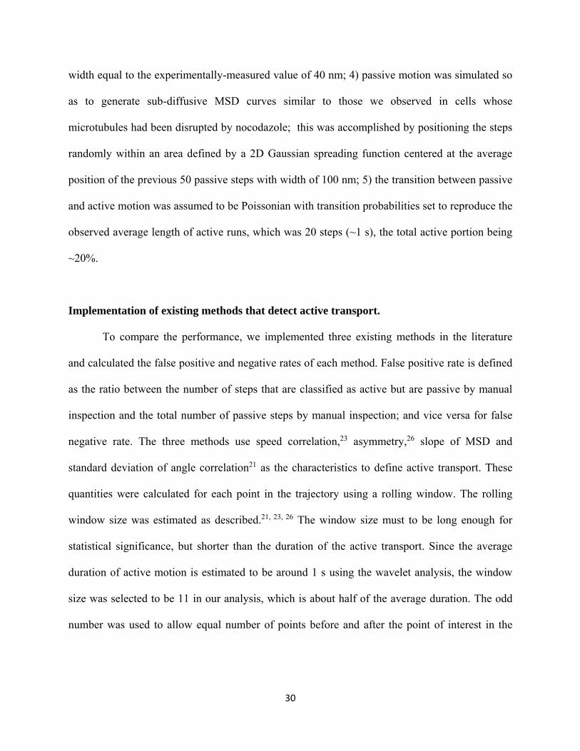
width equal to the experimentally-measured value of 40 nm; 4) passive motion was simulated so

as to generate sub-diffusive MSD curves similar to those we observed in cells whose

microtubules had been disrupted by nocodazole; this was accomplished by positioning the steps

randomly within an area defined by a 2D Gaussian spreading function centered at the average

position of the previous 50 passive steps with width of 100 nm; 5) the transition between passive

and active motion was assumed to be Poissonian with transition probabilities set to reproduce the

observed average length of active runs, which was 20 steps (~1 s), the total active portion being

~20%.

Implementation of existing methods that detect active transport.

To compare the performance, we implemented three existing methods in the literature

and calculated the false positive and negative rates of each method. False positive rate is defined

as the ratio between the number of steps that are classified as active but are passive by manual

inspection and the total number of passive steps by manual inspection; and vice versa for false

negative rate. The three methods use speed correlation,23 asymmetry,26 slope of MSD and

standard deviation of angle correlation21 as the characteristics to define active transport. These

quantities were calculated for each point in the trajectory using a rolling window. The rolling

window size was estimated as described.21, 23, 26 The window size must to be long enough for

statistical significance, but shorter than the duration of the active transport. Since the average

duration of active motion is estimated to be around 1 s using the wavelet analysis, the window

size was selected to be 11 in our analysis, which is about half of the average duration. The odd

number was used to allow equal number of points before and after the point of interest in the

31  

rolling window. The Lmax for the asymmetry method was set at 71 to match the longest possible

duration of active motion.

The thresholds for all three methods were determined from Brownian simulation. 100

Brownian trajectories of N=1000 frames with 20 fps were simulated for diffusion coefficient D =

0.001µm2s-1. The trajectories were composed of steps with a uniform probability distribution for

step direction and an exponential probability distribution for step length with a mean of 4D t .

For consistency with the literature,21, 23, 26 the threshold was defined for each parameter so that

99% of the simulated trajectories were classified as passive. These thresholds were designed to

include 1% false positives, but the real performance was worse according to our validation test.

The thresholds for speed correlation, asymmetry, slope of MSD and standard deviation of angle

correlation were 0.886, 1.25, 20.4 and 1.1 respectively. We verified that the thresholds were

sensitive to neither N nor D. When comparing the active assignment using these thresholds with

manual selection, we saw that fewer than 20% of the segments that were marked active manually

were identified as active by these methods. We therefore iteratively lowered the threshold for

each method until reaching a similar performance achieved by wavelet analysis (80-90% of the

segments that were marked active manually were identified as active by the respective method).

However, in doing so, we saw a sharp increase of false positive to ~20%.

Electrophoresis.

λ-DNA, covalently labeled by rhodamine (Mirus) was embedded within 1.5 wt% agarose

gel (Fisher, molecular biology grade, low EEO) in the presence of 1× TBE and glucose oxidase-

based anti-photobleaching buffer. Imaging and tracking details are published elsewhere.39 The

strength of the electric field was 6 to 12 V/cm.

32  

Colloid glass.

Briefly, the system involves tracking modulated optical nanoprobes (MOON) tracer

particles, prepared by coating a hemisphere of poly-methylmethacrylate (PMMA) particles with

12 nm of aluminum, in colloidal supercooled liquids comprised of PMMA colloids 1.42 μm in

diameter at volume fraction 0.51. The solvent is index-matched and density-matched. Bright

field imaging was used to track these probes as a function of time in four dimensions (x, y, in-

plane and out-plane angles), the metal side facing the objective appearing black. Details of the

experiments are published elsewhere.42

CTRW simulation.

To test wavelet analysis on anomalous diffusion that can be described as continuous time

random walk, we simulated trajectories for which the true statistics are known. For 1D

simulation in this spirit, exponentially distributed random numbers were generated for the step

size and the waiting times between steps were drawn from a power law distribution with

exponent 2. To this signal, noise was then added. Noise was generated from a normal distribution

with the standard deviation n , which is some multiple ( ) of the standard deviation s of the

step size distribution. For compound noise, two normally distributed random variables, each with

/ 2n s were added. For time varying noise, normally distributed random variables with

/ 2n s , n s and 2n s were added to the first, second and last 1/3 of the

trajectory.

SURE and Minimax were selected as the thresholding methods to compare with universal

thresholding because they are known to be less strict and their implementation is known to be

33  

computationally less expensive than other methods such as cross-validation.47 The thresholds

were calculated following literature.47, 50

 

2.5 References 1. Kusumi, A. et al. Paradigm shift of the plasma membrane concept from the two-dimensional

continuum fluid to the partitioned fluid: High-speed single-molecule tracking of membrane

molecules. Annual Review of Biophysics and Biomolecular Structure 34, 351-U354 (2005).

2. Barkai, E., Garini, Y. & Metzler, R. Strange kinetics of single molecules in living cells. Physics

Today 65, 29-35 (2012).

3. Moerner, W.E. New directions in single-molecule imaging and analysis. Proceedings of the

National Academy of Sciences of the United States of America 104, 12596-12602 (2007).

4. Brandenburg, B. & Zhuang, X. Virus trafficking - learning from single-virus tracking. Nature

Reviews Microbiology 5, 197-208 (2007).

5. Waigh, T.A. Microrheology of complex fluids. Reports on Progress in Physics 68, 685-742

(2005).

6. Wang, B., Kuo, J., Bae, S.C. & Granick, S. When Brownian diffusion is not Gaussian. Nature

Materials 11, 481-485 (2012).

7. Granick, S. et al. Single-molecule methods in polymer science. Journal of Polymer Science Part

B-Polymer Physics 48, 2542-2543 (2010).

8. Wong, I.Y. et al. Anomalous diffusion probes microstructure dynamics of entangled F-actin

networks. Physical Review Letters 92 (2004).

9. Cohen, A.E. & Moerner, W.E. Suppressing Brownian motion of individual biomolecules in

solution. Proceedings of the National Academy of Sciences of the United States of America 103,

4362-4365 (2006).

34  

10. Condamin, S., Tejedor, V., Voituriez, R., Benichou, O. & Klafter, J. Probing microscopic origins

of confined subdiffusion by first-passage observables. Proceedings of the National Academy of

Sciences of the United States of America 105, 5675-5680 (2008).

11. Wang, B. et al. Confining potential when a biopolymer filament reptates. Physical Review Letters

104 (2010).

12. Weeks, E.R., Crocker, J.C., Levitt, A.C., Schofield, A. & Weitz, D.A. Three-dimensional direct

imaging of structural relaxation near the colloidal glass transition. Science 287, 627-631 (2000).

13. Cheng, X., McCoy, J.H., Israelachvili, J.N. & Cohen, I. Imaging the microscopic structure of

shear thinning and thickening colloidal suspensions. Science 333, 1276-1279 (2011).

14. Turchin, P. Quantitative analysis of movement: measuring and modeling population redistribution

in animals and plants. (Sinauer Associates, Incorporated, 1998).

15. Zhao, K. et al. Psl trails guide exploration and microcolony formation in Pseudomonas aeruginosa

biofilms. Nature 497, 388-391 (2013).

16. Suh, J., Wirtz, D. & Hanes, J. Efficient active transport of gene nanocarriers to the cell nucleus.

Proceedings of the National Academy of Sciences of the United States of America 100 (2003).

17. Jaqaman, K. et al. Robust single-particle tracking in live-cell time-lapse sequences. Nature

Methods 5, 695-702 (2008).

18. Zhu, L., Zhang, W., Elnatan, D. & Huang, B. Faster STORM using compressed sensing. Nature

Methods 9, 721-U286 (2012).

19. Sahl, S.J., Leutenegger, M., Hilbert, M., Hell, S.W. & Eggeling, C. Fast molecular tracking maps

nanoscale dynamics of plasma membrane lipids. Proceedings of the National Academy of

Sciences of the United States of America 107, 6829-6834 (2010).

20. Liao, Y., Yang, S.K., Koh, K., Matzger, A.J. & Biteen, J.S. Heterogeneous single-molecule

diffusion in one-, two-, and three-dimensional microporous coordination polymers: directional,

trapped, and immobile guests. Nano Letters 12, 3080-3085 (2012).

35  

21. Arcizet, D., Meier, B., Sackmann, E., Raedler, J.O. & Heinrich, D. Temporal analysis of active

and passive transport in living cells. Physical Review Letters 101 (2008).

22. Monnier, N. et al. Bayesian approach to MSD-based analysis of particle motion in live cells.

Biophysical Journal 103, 616-626 (2012).

23. Bouzigues, C. & Dahan, M. Transient directed motions of GABA(A) receptors in growth cones

detected by a speed correlation index. Biophysical Journal 92 (2007).

24. Thompson, M.A., Casolari, J.M., Badieirostami, M., Brown, P.O. & Moerner, W.E. Three-

dimensional tracking of single mRNA particles in Saccharomyces cerevisiae using a double-helix

point spread function. Proceedings of the National Academy of Sciences of the United States of

America 107, 17864-17871 (2010).

25. Tuerkcan, S., Alexandrou, A. & Masson, J.-B. A Bayesian Inference scheme to extract diffusivity

and potential fields from confined single-molecule trajectories. Biophysical Journal 102, 2288-

2298 (2012).

26. Huet, S. et al. Analysis of transient behavior in complex trajectories: Application to secretory

vesicle dynamics. Biophysical Journal 91 (2006).

27. Zaliapin, I., Semenova, I., Kashina, A. & Rodionov, V. Multiscale trend analysis of microtubule

transport in melanophores. Biophysical Journal 88, 4008-4016 (2005).

28. Tejedor, V. et al. Quantitative analysis of single particle trajectories: mean maximal excursion

method. Biophysical Journal 98, 1364-1372 (2010).

29. McKinney, S.A., Joo, C. & Ha, T. Analysis of single-molecule FRET trajectories using hidden

Markov modeling. Biophysical Journal 91, 1941-1951 (2006).

30. Mallat, S. A wavelet tour of signal processing. (Elsevier Science, 1999).

31. Percival, D.B. & Walden, A.T. Wavelet methods for time series analysis. (Cambridge University

Press, 2006).

32. Ivanov, P.C. et al. Scaling behaviour of heartbeat intervals obtained by wavelet-based time-series

analysis. Nature 383, 323-327 (1996).

36  

33. Yang, H. Detection and characterization of dynamical heterogeneity in an event series using

wavelet correlation. Journal of Chemical Physics 129 (2008).

34. Taylor, J.N., Makarov, D.E. & Landes, C.F. Denoising single-molecule FRET trajectories with

wavelets and bayesian inference. Biophysical Journal 98, 164-173 (2010).

35. Taylor, J.N. & Landes, C.F. Improved resolution of complex single-molecule FRET systems via

wavelet shrinkage. Journal of Physical Chemistry B 115, 1105-1114 (2011).

36. Vale, R.D. The molecular motor toolbox for intracellular transport. Cell 112, 467-480 (2003).

37. Mueller, M.J.I., Klumpp, S. & Lipowsky, R. Tug-of-war as a cooperative mechanism for

bidirectional cargo transport by molecular motors. Proceedings of the National Academy of

Sciences of the United States of America 105, 4609-4614 (2008).

38. Wang, B. in Materials Science and Engineering, Vol. Doctor of Philosophy (University of Illinois

at Urbana-Champaign, 2011).

39. Guan, J., Wang, B., Bae, S.C. & Granick, S. Modular stitching to image single-molecule DNA

transport. Journal of the American Chemical Society 135, 6006-6009 (2013).

40. Dorfman, K.D., King, S.B., Olson, D.W., Thomas, J.D.P. & Tree, D.R. Beyond gel

electrophoresis: microfluidic separations, fluorescence burst analysis, and DNA stretching.

Chemical reviews 113, 2584-2667 (2013).

41. Kegel, W.K. & van Blaaderen, A. Direct observation of dynamical heterogeneities in colloidal

hard-sphere suspensions. Science 287, 290-293 (2000).

42. Kim, M., Anthony, S.M., Bae, S.C. & Granick, S. Colloidal rotation near the colloidal glass

transition. Journal of Chemical Physics 135 (2011).

43. Tabei, S.M.A. et al. Intracellular transport of insulin granules is a subordinated random walk.

Proceedings of the National Academy of Sciences of the United States of America 110, 4911-4916

(2013).

37  

44. Weigel, A.V., Simon, B., Tamkun, M.M. & Krapf, D. Ergodic and nonergodic processes coexist

in the plasma membrane as observed by single-molecule tracking. Proceedings of the National

Academy of Sciences of the United States of America 108, 6438-6443 (2011).

45. Montroll, E.W. & Weiss, G.H. Random walks on lattices .2. Journal of Mathematical Physics 6,

167-& (1965).

46. Calderon, C.P., Harris, N.C., Kiang, C.-H. & Cox, D.D. Quantifying multiscale noise sources in

single-molecule time series. Journal of Physical Chemistry B 113, 138-148 (2009).

47. Donoho, D.L. & Johnstone, I.M. Ideal spatial adaptation by wavelet shrinkage. Biometrika 81,

425-455 (1994).

48. Tokunaga, M., Imamoto, N. & Sakata-Sogawa, K. Highly inclined thin illumination enables clear

single-molecule imaging in cells. Nature Methods 5, 159-161 (2008).

49. Anthony, S., Zhang, L.F. & Granick, S. Methods to track single-molecule trajectories. Langmuir

22, 5266-5272 (2006).

50. Donoho, D.L. & Johnstone, I.M. Adapting to unknown smoothness via wavelet shrinkage.

Journal of the American Statistical Association 90, 1200-1224 (1995).

38  

CHAPTER 3

EXTENDING PARTICLE TRACKING CAPABILITY

WITH DELAUNAY TRIANGULATION

3.1 Background

We are in the midst of an imaging revolution. Going beyond the older use of images to

provide primarily qualitative information (important as that is), rapid developments are

underway in quantitative imaging – the standardized quantification of large statistical datasets,

often from time series of images, and usually enabled by rapid computer processing. While

particle tracking of moving objects in time series of images has become routine,1, 2 a great

limitation is that the standard particle tracking analyzes diffraction-limited spots, for example in

single-molecule studies.3, 4 This study concerns three significant limitations of the standard

methods: first, difficulty to separate reliably objects that are in close proximity; second,

difficulty to identify the same moving element in time series in which there are some missing

frames; third, difficulty to describe irregular, asymmetric shapes. This chapter explains how to

extend these capabilities using Delaunay triangulation in ways that are computationally efficient

and easy to implement with common software packages.

                                                              Adapted with permission from Stephen M. Anthony, and Steve Granick (2014) Extending particle

tracking capability with Delaunay triangulation, Langmuir, 30, 4760-4766. Copyright 2014 American

Chemical Society.

 

39  

The technical problem is the following. While to identify different objects in an image

often seems obvious to one’s eyes, identifying them automatically using computers for

quantitative analysis is often hampered by noise in the image, irregularity of shapes, and

proximity of objects. The first step to separate objects is to identify the pixels that comprise each

object, but in general it is not possible to identify all points correctly, not when there is low

signal-to-noise and intensity variation within an object. This precludes simple grouping by

connectivity. When dealing with objects of irregular shape, to separate them becomes more

difficult. Standard clustering techniques such as K-means and hierarchical have limitations: K-

means5 is only suitable for spherical shapes with similar sizes and hierarchical6 works only when

all the objects have similar shape (detailed comparisons are presented below). Difficulties arise

when the objects are highly non-spherical and random; it is a serious problem as this class

includes important moving objects such as the polymer chains,7, 8 rod-like bacteria,9 highly-

branched neurons,10 and irregular domains in phase separation.11

After one succeeds in identifying objects quantitatively and pixel-wise, connecting the

position of an object from one frame to the next can reveal useful information about the

dynamics of motion. But this is problematical to do, because connecting objects between frames

to build up trajectories can be difficult when the object disappears from view for a few frames

before becoming visible again, which is common due to blinking of fluorophores and diffusion

in and out of the focal plane. If, in analysis, one decides to terminate each trajectory when the

moving object becomes invisible, this will improperly bias the data towards short trajectories and

will interfere with accumulating information about long time dynamics. There are attempts to

connect the gaps in time after linking particles in adjacent frames.17, 18 The new method proposed

here simultaneously connects the gaps in space and in time. A better method to bridge time gaps

40  

may also further improve the performance of super-resolution imaging techniques, such STORM

and PALM, by combining the signal that single fluorophores present during different activation

cycles.

Another application of Delaunay triangulation is in the study of shapes that change with

time: for example, the quantification of cell shape12 and polymer chains configurations.13 While

center of mass motion is the standard quantity of which to keep track,14, 15 a good descriptor for

shape is less obvious. Principal axes,7 moments,16 ellipticity,17, 18 and degree of asymmetry19 are

some of the metrics that have been used to describe shapes. While each captures some important

aspects of the shape, such single-number quantifications cannot describe internal degrees of

freedom, such as twists and turns within the shape. But it is not helpful to go to the other extreme

and retain for analysis all the points in an object; if the information retained is too large, changes

of the same shape cannot be discriminated either. The backbone of objects strikes a fine balance

between keeping too few and too many details.

Graph theory, developed in mathematics and computer science, contains tools useful for

these problems. Delaunay triangulation, one such tool, divides a space into sub-regions

according to the rule that the circumcircle of any triangle must be empty (Fig. 3.1). Possessing

the unique property that all nearest neighbors are connected, it quantifies spatial proximity very

well, and as spatial proximity is the physical basis for clustering points, this explains why

Delaunay triangulation is widely used in urban and geological studies to aggregate feature

points.20

41  

Figure 3.1. Example of performing Delaunay triangulation on four points in a plane. The

triangulation in (a) is correct because the circumcircles (blue) of both triangles (red) exclude the

fourth point (green). Case (b) shows an incorrect triangulation where the circumcircles of both

triangles contain the fourth point. This tutorial example generalizes to arbitrarily-large numbers

of points. The text discusses the example of multidimensional space where one axis is position

and a second axis is time. (c) Comparison of computation time using Delaunay triangulation

(blue) and brute force strategy (red) of calculating the distance between all points on an image..

While the brute force approach is independent of the dimension, 3D takes longer (blue solid line)

than 2D (blue dash line) for Delaunay triangulation. The brute force approach is relatively

advantageous only for 3D trajectories containing few points (3D: two spatial coordinates plus

time), as discussed further in the supplementary material.

 

As we show below and illustrate in detail, this method applies efficiently when the time

variable is added. In this argument, the concept of spatial proximity extends to connecting

trajectories; one considers time as an additional dimension orthogonal to space, defining the

distance between two points as a combination of their distances in space and time, thus

42  

augmenting the effectiveness of particle tracking through intervening times. The application to

identifying backbones of objects follows similarly, as the minimum spanning tree, defined

below, of the graph of all distances for a set of points is a sub-graph of their Delaunay

triangulation.21 In this study, we demonstrate how Delaunay triangulation can be applied to these

problems and how the performances compare with existing methods.

3.2 Methods

Separating objects.

The process of separating objects includes four steps: (1) selecting an intensity threshold

and binarizing the image according to this threshold; the threshold is typically selected as n

standard deviations above the average intensity of the image. Here, for physical reasons one

selects n depending on the signal-to-noise ratio of the image. (2) Performing Delaunay

triangulation (Fig. 3.2c) on the points in the binarized image (Fig. 3.2b); this is done using the

built-in function in common software, for example “Delaunay” when one uses Matlab. (3)

Selecting a threshold for the maximum distance between two neighboring points in the same

object and removing edges in the Delaunay triangulation that exceed the threshold (Fig. 3.2e);

and (4) grouping the connected points by the remaining edges (Fig. 3.2h).

43  

Figure 3.2. Example of separating actin filaments in a fluorescence image (images taken from

ref. 7). The raw image (a) is first binarized (b) and a Delaunay triangulation (DT) (c) is

constructed on the points that were set to unity in the binarized image. Different edge thresholds

were used to remove the long edges (red) and the remaining edges (blue) are shown in (d-f).

Finally points that are connected by the remaining edges are grouped together (g-i). Each group

is represented by a different color. Proper threshold (“thld”) choice (h) is important, as

depending upon the threshold chosen, either oversegmentation (g) or undersegmentation (i)

segmentation may occur. (j-l) shows the results obtained using other clustering functions

available in Matlab: k-means, fussy c-means, and hierarchical.

44  

To achieve successful separation, the choice of appropriate threshold is critical. The

performance of the method depends on two competing factors: the separation between objects

and the gap within an object. The higher the ratio between the two, the less sensitive the method

is to the choice of threshold. Too low a threshold can cause objects to be artificially fragmented

(Fig. 3.2d, g) while too high a threshold can cause nearby objects to artificially cluster together

(Fig. 3.2f, i). It is often necessary to iteratively test different candidate threshold values to obtain

one that works the best. In Fig. 3.2, we purposely illustrate a very challenging example with two

objects being very close at the bottom of the image and with part of the largest object in the

bottom left corner of the image not being as bright as the rest so that the object becomes

fragmented by binarization. This example gives a ratio close to 1, which approaches the limit of

the method. Therefore we see a high sensitivity to the threshold value, as expected, but to

mitigate this problem one can exploit the special properties of the edges linking two objects.20

Zooming in (Fig. 3.3a), one notices that the edges that connect the two objects are substantially

longer than neighboring edges. Based on this observation, one can remove such edges by

comparing edge lengths locally. For each point, if an edge connects to this point exceeds a local

threshold, the edge is removed. The local threshold is then determined by:20

2threshold (P ) = mean (P )+ mean_variation( ) ij G j iG (1)

where 2mean (P )iG j is the mean length of the edges formed by the points in the second-order

neighbors of point Pj . Second order neighboring points provide a window to look at local

details. Furthermore, can be tuned to adjust sensitivity to local variations. Since the number of

edges formed by second order neighboring points can be small, the error associated with

calculating variations can become significant. Therefore, the mean variation of all the sub-graphs

mean_variation( ) iG is used as the variation indicator.

45  

Another type of local inconsistency can be links between clusters as shown in the

example in Fig. 3.3c. Consider the point circled in red in Fig. 3.3d, it has multiple second-order

neighbors to the left, but only one to the right. One way to quantitatively capture this is to

introduce the idea of local aggregation force,20 which sums up vectorially the influence of the

second-order points on a given point:

2,2

1, ,

, j k ij k P P k G j

j k

F P P e P N Pd P P

(2)

while the direction of the vector ,j kP Pe

is determined by the positions of the points. The length of

the vector should be inversely proportional to the distance between the two points so that points

located far away have lesser influence, hence the normalization by 2 ,j kd P P . Summing up the

individual local aggregation force gives the cohesive local aggregation force on a point:

2, ,i

t j j k k G jF P F P P P N P

(3)

As seen from Fig. 3.3d, the cohesive aggregation force on point located on the border of a cluster

point to the interior of that cluster. This causes the point to have a tendency to move into the

cluster and implies that the edge pointing to the opposite direction should be removed.

Mathematically, this is done by looking at the angles between the cohesive aggregation force

vector and the vector between the point and its first-order neighbors. When angles exceed a

reasonable threshold, 150˚ for this example, then the edge is removed. For points in the interior

of the cluster, the magnitude of the cohesive aggregation force should be very small as the forces

due to neighbors in opposite directions cancel each other. The direction of the cohesive

aggregation force is therefore random and removing edges using the above criterion can result in

arbitrary segmentation of the cluster. To avoid this, the angle criterion is only applied to points

46  

with cohesive aggregation force greater than a set threshold so that all edges in the interior of

clusters are not affected, as seen in Fig. 3.3e.

Figure 3.3. Examples of local removal of inconsistent edges. (a) This shows a zoom-in of the

boxed area in Fig. 3.2f. Edges formed by second-order neighbors of the asterisk point are

highlighted in red. (b) This shows the result after removal, from (a), of long local edges. (c) This

shows an example of local link edges removal. (d) This shows the cohesive aggregation force of

the circled point. (e) Edges that point in the opposite direction from the cohesive aggregation

forces are removed. (f) This shows the final clustering result.

Connecting trajectories.

The same procedure can connect trajectories, the only difference being that instead of

using a threshold to identify feature points as would be seen by one’s eyes, a new coordinate

47  

system defines trajectory points. The idea is that a trajectory can be viewed as an object whose

points lie in a temporal-spatial coordinate system.

Consider the simulated example in Fig. 3.4; two particles diffuse in a micron-sized 1D

system and are observed every 1 ms. The two trajectories are easily identified by frame-to-frame

spatial comparison, except for the problematical last point where there is a time gap. This is an

example of the usefulness of Delaunay triangulation, as both of these trajectories can reach the

last point through either a jump in space or time. A “slowly” moving object is most likely to

move a short distance even after a long time elapses; it is unlikely to move a long distance

quickly. Conversely, a “rapidly” moving object is most likely to move a long distance quickly; it

is unlikely to remain for a long time near the same location. To determine which is more likely

quantitatively, we begin by selecting a conversion factor for time and forming a 2D coordinate

system with time as the orthogonal axis. Having established the equivalent scales of the temporal

and spatial axes, we then assess, from the relative distance between points in this 2D space, the

relative likelihood of the options. But as the distance between orthogonal points depends on the

equivalent scales of the axes on which they sit, how to set their equivalent scales requires

judicious thinking. The best choices of equivalent scales depend on the physical problem at

hand. When the motion is ballistic or has persistent direction, such as active transport of

endosomes by molecular motors along microtubules or the electrophoresis of DNA chains where

there is a well-defined velocity, the obvious conversion factor between space and time is the

velocity. One can multiply the time data with the velocity to convert to spatial units. For

example, if the velocity is 100 nm/s, then 10 ms will be converted to 1 nm, so 10 ms in the

temporal dimension should have the same length as 1 nm in the spatial dimension.

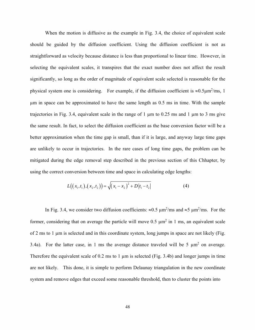
48  

When the motion is diffusive as the example in Fig. 3.4, the choice of equivalent scale

should be guided by the diffusion coefficient. Using the diffusion coefficient is not as

straightforward as velocity because distance is less than proportional to linear time. However, in

selecting the equivalent scales, it transpires that the exact number does not affect the result

significantly, so long as the order of magnitude of equivalent scale selected is reasonable for the

physical system one is considering. For example, if the diffusion coefficient is 0.5µm2/ms, 1

µm in space can be approximated to have the same length as 0.5 ms in time. With the sample

trajectories in Fig. 3.4, equivalent scale in the range of 1 µm to 0.25 ms and 1 µm to 3 ms give

the same result. In fact, to select the diffusion coefficient as the base conversion factor will be a

better approximation when the time gap is small, than if it is large, and anyway large time gaps

are unlikely to occur in trajectories. In the rare cases of long time gaps, the problem can be

mitigated during the edge removal step described in the previous section of this Chhapter, by

using the correct conversion between time and space in calculating edge lengths:

2

1 1 2 2 1 2 1 2, , ,L x t x t x x D t t (4)

 

In Fig. 3.4, we consider two diffusion coefficients: 0.5 µm2/ms and 5 µm2/ms. For the

former, considering that on average the particle will move 0.5 µm2 in 1 ms, an equivalent scale

of 2 ms to 1 µm is selected and in this coordinate system, long jumps in space are not likely (Fig.

3.4a). For the latter case, in 1 ms the average distance traveled will be 5 µm2 on average.

Therefore the equivalent scale of 0.2 ms to 1 µm is selected (Fig. 3.4b) and longer jumps in time

are not likely. This done, it is simple to perform Delaunay triangulation in the new coordinate

system and remove edges that exceed some reasonable threshold, then to cluster the points into

49  

Figure 3.4. A 1D simulated trajectory to illustrate how Delaunay triangulation applies to

trajectories with missing frames. The 1D trajectories (red and green) are plotted in 2D with time

as the orthogonal dimension. The problem is to decide, to which trajectory does the last point in

time belong? If passage in time is given a relatively small length (a), the jump in space is

relatively large and the last point should belong to the red trajectory on physical grounds. Using

Delaunay triangulation, after removing the long edges, the last point indeed is connected to the

red trajectory. But if the passage in time is given a relatively large length (b), the last point would

be assigned to belong to the green trajectory.

trajectories. In this case, the competing factors are: the separation between points that belong to

different particles and the gap between points that belong to the same particles. Local edge

removal can again be applied to reduce sensitivity to the value of threshold with which the

analysis begins. Note that in this example, for all but the last point, the trajectories identified by

the Delaunay triangulation using either equivalent scale are the same as those connected by

frame-to-frame comparison. Therefore Delaunay triangulation can connect the trajectories on its

50  

own and one does not need to use it together with frame-to-frame comparison. The advantage of

Delaunay triangulation is that it provides a rational decision of how to treat the final point of the

trajectory. If the edges connecting the final point to both trajectories turn out to be too long, then

the final point will be assigned as the start of a new trajectory. Physically, this could happen

when a new particle enters the field of view, and hence becomes a useful method to discriminate

genuine new particles from older particles that had momentarily disappeared from view.

Identifying backbones.

Whereas after isolating an object, simple spline curve fitting can identify its backbone

provided that it does not contain sharp turns, this works poorly for objects with sharp turns, such

as the DNA molecule in Fig. 3.5a. Delaunay triangulation is helpful in such cases. Two

additional steps are needed after performing Delaunay triangulation on the points of an object:

(1) find the minimum spanning tree of the edges from the Delaunay triangulation; (2) locate the

longest path in the minimum spanning tree. A minimum spanning tree is a subgraph that

connects all the vertices of a graph with the lowest weight. Mathematically, the minimum

spanning tree for the complete graph of the distances between the vertices is known to be a

subset of the Delaunay triangulation of the same set of vertices.21 It is part of common software

packages. For example, in the MatlabBGL graph library22 used for the current study, the

function called “mst” calculates the minimum spanning tree of a graph.

The backbone of the object should simultaneously minimize both the length of the path

connecting the two ends of the object and the extent of the excursions away from the backbone

required to reach all other points. The subset of the edges forming the longest path in the

minimum spanning tree provides a good approximation of the optimal backbone, tending to

51  

balance these two competing optimizations. By definition, the minimum spanning tree between

any pair of points will take the shortest path between those points except when adding additional

intermediate points result in a reduction in the length of the paths required to connect the

remaining points in the graph.

When computing the minimum spanning tree, it is critical to use intensity-weighted edge

lengths:

2, , exp j kw j k j k

I IL P P d P P

I

(5)

where I is the average intensity of all the points. This is because if simple Euclidean edge

lengths were used, as in Fig. 3.5c, in many subregions of the graph the minimum spanning tree

would be highly degenerate. Even if the degeneracy could be broken when considering larger

graphs, perhaps the entire graph, and even if this produced a unique minimum spanning tree, the

result would be artificial for the following reason. The structure of the minimum spanning tree

depends most strongly on pixels at the edges of the thresholded region; therefore the longest path

within the minimum spanning tree exhibits significant randomness and is likely to be off center

(Fig. 3.5c). In contrast, when considering the intensity warped space, distances between high

intensity points are relatively shorter than between dimmer ones. Therefore the shortest path

preferentially includes the brighter pixels (Fig. 3.5d). In addition to producing better and more

robust results, weighing algorithms that favor edges between bright pixels are physically

reasonable because in experiments based on fluorescence imaging, the local intensity normally

depends on the local density of fluorophores.

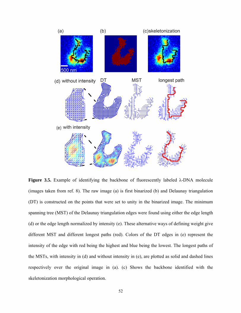
52  

Figure 3.5. Example of identifying the backbone of fluorescently labeled λ-DNA molecule

(images taken from ref. 8). The raw image (a) is first binarized (b) and Delaunay triangulation

(DT) is constructed on the points that were set to unity in the binarized image. The minimum

spanning tree (MST) of the Delaunay triangulation edges were found using either the edge length

(d) or the edge length normalized by intensity (e). These alternative ways of defining weight give

different MST and different longest paths (red). Colors of the DT edges in (e) represent the

intensity of the edge with red being the highest and blue being the lowest. The longest paths of

the MSTs, with intensity in (d) and without intensity in (e), are plotted as solid and dashed lines

respectively over the original image in (a). (c) Shows the backbone identified with the

skeletonization morphological operation.

53  

Note: this result is insensitive to the exact form of the intensity weighting. We tried an

alternative approach to define the intensity-weighted edge lengths, Eq. (6), and obtained the

exact same result:

2 ,,

j k

w j kj k

d P PL P P

I I

(6)

 

3.3 Discussions: Comparison with alternative methods

Separating objects.

Given a set of points corresponding to different objects, while it should be possible in

principle to calculate by brute force the pairwise separation distances rather than perform

Delaunay triangulation, to do so can be very computationally expensive and easily exceeds the

maximum computer memory when the number of points is large.

A quantitative comparison of computational time was presented in Fig. 3.1c. The

computational time grows nearly linearly with the number of points for Delaunay triangulation,

but for the brute force strategy it grows quadratically, with more details given in the

Supplementary Information. The reason for the near linear computational time for Delaunay

triangulation is that sub-graphs of the triangulation are insensitive to vertices far away from the

region. Various algorithms exploited this property. For example, the divide and conquer

algorithm recursively draws a line to split the vertices into two set and compute the Delaunay

triangulation for each set. The two sets are then merged along the splitting line and with fast

merge operation, the total running time is O(nlogn).23 In terms of memory requirements for

computation, empirically we observed that in Matlab while 100,000 data points require only

about 1.6 GB of RAM when using Delaunay triangulation, 30,000 points computed using brute

force already require more than 24 GB of RAM, which exceeds what common computers have.

54  

To put this into perspective, readers should consider that 30,000 data points are commonly

acquired in typical particle tracking experiments. This is evident when one considers that

particle tracking typical spans at least 1000 frames with 10s or even 100s of objects in each

frame. Brute force calculation is therefore prohibitively demanding for efficient computation.

To separate objects, an important advantage of Delaunay triangulation is that, unlike

other clustering methods, it makes no assumption about the shape, size distribution, or number of

objects. For example, K-means5 requires the number of clusters as an input and cannot separate

the objects correctly unless this input is correct. It then assigns all points to the cluster centers to

which they are closest and iteratively updates the centers until the total distance is minimized. K-

means effectively divides space into spherical regions; when dealing with nonspherical objects,

parts of an object can be unwittingly assigned to the circle of another object. This was clearly

seen in Fig. 3.2j. Similarly, if there is a wide distribution of object sizes, parts of a large object

might be closer to the center of a nearby small object than to its own center, resulting in mistaken

identification. These problems limit the usefulness of K-means to spherical objects with similar

sizes. In spite of these limitations, K-means is used fairly frequently in the current literature

because of its ease of implementation. In this study, we emphasize that Delaunay triangulation

can do better. The methods presented here can be implemented easily because most common

software packages contain implementations of Delaunay triangulation. For example, to

accomplish Delaunay triangulation we routinely employ Matlab and compute the minimum

spanning tree using the MatlabBGL graph library.22

One limitation of using Delaunay triangulation to separate objects, which is also a

limitation for other clustering techniques, is that when two objects are very close, it becomes

difficult to separate them. This can be mitigated by inspecting locally to remove edges that are

55  

longer than their neighbors and also edges that link two objects, using the methods that we have

described in detail above. By setting a relatively high threshold globally and removing local

inconsistencies afterwards, the combination of Delaunay triangulation with local edge removal

can be robustly applied to processing large datasets.

Connecting trajectories.

Beyond this, Delaunay triangulation is a natural solution to the endemic problem of how

to connect missing frames in trajectories. When it comes to connecting trajectories, it is true that

frame-to-frame comparison can be extended to include neighboring frames if frequent frames are

missing, but this requires arbitrary judgment, such as how many neighboring frames to include,

and what to do when a point is closer to the current point in space than another point, yet is

further removed in time. Delaunay triangulation condenses all the above considerations into the

single question of equivalence scales of the temporal and spatial axes. This makes the problem

much easier and more quantitative to approach. For example, for the special case of

STORM24 experiments, the experimental design ensures that the spatial positions of the

fluorophores do not change, so the temporal scale can be set to be much smaller than the spatial

scale to make jumps in space very unlikely, and this assists in closing gaps in time. This is in the

same spirit as the maximum likelihood based statistical method to find the most likely set of

fluorophore positions.25 As in separating objects, when two points are too close, Delaunay

triangulation can combine the respective trajectories to which they belong and the same local

edge removal steps can be used to separate the trajectories.

To extend this method to higher dimensional data (such as 4D, three spatial dimensions

and 1 time dimension) is easily accomplished. In Matlab, one uses the provided N-dimensional

56  

Delaunay triangulation function “delaunayn”. Alternatively, Qhull provides a freely available,

open source implementation of the Quickhull algorithm,26 a commonly used N-dimensional

delaunay triangulation algorithm. Within Mathematica, an interface intended to facilitate the use

of Qhull is provided by Wolfram Research.

Identifying backbones.

There exist alternative, well-established skeletonization methods that work well when all

the pixels of an object can be identified, in other words when there are no holes and scattered

points due to noise or non-uniformity.27 However, often this is not the case with fluorescence or

bright field images because labeling intensity and refractive index can vary from point to point.

The current method based on Delaunay triangulation has a higher tolerance of missing points as

the general structure of the minimums spanning tree is not easily affected by a few missing

points. Another advantage over morphological methods is that the current method is able to take

into account the pixel intensities. It is interesting that the morphological operation of

skeletonization (Fig. 3.5c) gives the same backbone as the minimum spanning tree without

intensity normalization. The comparison highlights the importance of using the intensity

information when seeking to identify the backbone of an object.

As an alternative when points in an object are scattered, the most competitive alternative

to Delaunay triangulation is probably the B-spline,28 which fit a smooth curve to the point cloud.

Variations of B-spline curve fitting exist29 but generally, B-spline based methods have difficulty

when dealing with sharp turns or large thickness variation along the backbone.30 The minimum

spanning tree of Delaunay triangulation is less sensitive to these issues. But a limitation of using

backbone as a representation of object shape is that when objects are close to spherical there is

57  

not well-defined longest path, so there is no unique backbone. Another limitation is that the

method is most accurate within objects, less so towards their ends.

3.4 Conclusions

The proposed methods can enhance the current capabilities of particle tracking

algorithms by allowing irregular shaped objects to be separated and have their shape

characterized by the backbone, as well as providing an easy way to connect trajectories with

frequent missing frames. Applications that can gain the most benefit by adopting these methods

include: single molecule studies of polymer conformation dynamics,13 cell morphology studies,12

and super-resolution imaging techniques that are based on photo-activation cycles.24

3.5 References

1. Dupont, A. & Lamb, D.C. Nanoscale three-dimensional single particle tracking. Nanoscale 3,

4532-4541 (2011).

2. Saxton, M.J. & Jacobson, K. Single-particle tracking: Applications to membrane dynamics.

Annual Review of Biophysics and Biomolecular Structure 26, 373-399 (1997).

3. Moerner, W.E. New directions in single-molecule imaging and analysis. Proceedings of the

National Academy of Sciences of the United States of America 104, 12596-12602 (2007).

4. Xia, T., Li, N. & Fang, X. Single-molecule fluorescence imaging in living cells. Annual Review

of Physical Chemistry, Vol 64 64, 459-480 (2013).

5. Jain, A.K. Data clustering: 50 years beyond K-means. Pattern Recognition Letters 31, 651-666

(2010).

6. Estivill-Castro, V. & Lee, I. Multi-level clustering and its visualization for exploratory spatial

analysis. Geoinformatica 6, 123-152 (2002).

58  

7. Hsieh, C.-C., Balducci, A. & Doyle, P.S. An experimental study of DNA rotational relaxation

time in nanoslits. Macromolecules 40, 5196-5205 (2007).

8. Guan, J., Wang, B. & Granick, S. Automated single-molecule imaging to track DNA shape.

Langmuir 27, 6149-6154 (2011).

9. Zhao, K. et al. Psl trails guide exploration and microcolony formation in Pseudomonas aeruginosa

biofilms. Nature 497, 388-391 (2013).

10. Micheva, K.D., Busse, B., Weiler, N.C., O'Rourke, N. & Smith, S.J. Single-synapse analysis of a

diverse synapse population: proteomic imaging methods and markers. Neuron 68, 639-653

(2010).

11. Jensen, M.H., Morris, E.J. & Simonsen, A.C. Domain shapes, coarsening, and random patterns in

ternary membranes. Langmuir 23, 8135-8141 (2007).

12. Joshi, S.D., Kim, H.Y. & Davidson, L.A. Microscopy tools for quantifying developmental

dynamics in Xenopus embryos. Methods in molecular biology (Clifton, N.J.) 917, 477-493

(2012).

13. Levy, S.L., Mannion, J.T., Cheng, J., Reccius, C.H. & Craighead, H.G. Entropic unfolding of

DNA molecules in nanofluidic channels. Nano Letters 8, 3839-3844 (2008).

14. Walder, R., Kastantin, M. & Schwartz, D.K. High throughput single molecule tracking for

analysis of rare populations and events. Analyst 137, 2987-2996 (2012).

15. Flier, B.M.I. et al. Single molecule fluorescence microscopy investigations on heterogeneity of

translational diffusion in thin polymer films. Physical Chemistry Chemical Physics 13, 1770-

1775 (2011).

16. Shimada, J. & Yamakawa, H. Moments for dna topoisomers - the helical wormlike chain.

Biopolymers 27, 657-673 (1988).

17. Rosin, P.L. Measuring shape: ellipticity, rectangularity, and triangularity. Machine Vision and

Applications 14, 172-184 (2003).

59  

18. Aktas, M.A. & Zunic, J. Measuring shape ellipticity. Computer Analysis of Images and Patterns:

14th International Conference, Caip 2011, Pt I 6854, 170-177 (2011).

19. Klingenberg, C.P., Barluenga, M. & Meyer, A. Shape analysis of symmetric structures:

Quantifying variation among individuals and asymmetry. Evolution 56, 1909-1920 (2002).

20. Deng, M., Liu, Q., Cheng, T. & Shi, Y. An adaptive spatial clustering algorithm based on

delaunay triangulation. Computers Environment and Urban Systems 35, 320-332 (2011).

21. Aurenhammer, F. Voronoi diagrams - a survey of a fundamental geometric data structure.

Computing Surveys 23, 345-405 (1991).

22. Gleich, D. Boost C++ Libraries (http://www.boost.org/).

23. Cignoni, P., Montani, C. & Scopigno, R. DeWall: A fast divide and conquer Delaunay

triangulation algorithm in E-d. Computer-Aided Design 30, 333-341 (1998).

24. Rust, M.J., Bates, M. & Zhuang, X. Sub-diffraction-limit imaging by stochastic optical

reconstruction microscopy (STORM). Nature Methods 3, 793-795 (2006).

25. Mukamel, E.A., Babcock, H. & Zhuang, X. Statistical deconvolution for superresolution

fluorescence microscopy. Biophysical Journal 102, 2391-2400 (2012).

26. Barber, C.B., Dobkin, D.P. & Huhdanpaa, H. The Quickhull algorithm for convex hulls. Acm

Transactions on Mathematical Software 22, 469-483 (1996).

27. Lam, L., Lee, S.W. & Suen, C.Y. Thinning methodologies - a comprehensive survey. Ieee

Transactions on Pattern Analysis and Machine Intelligence 14, 869-885 (1992).

28. Eilers, P.H.C. & Marx, B.D. Flexible smoothing with B-splines and penalties. Statistical Science

11, 89-102 (1996).

29. Lee, E.T.Y. Comments on some b-spline algorithms. Computing 36, 229-238 (1986).

30. Liu, Y., Yang, H.P., Wang, W.P. & Society, I.C. Reconstructing B-spline curves from point

clouds - A tangential flow approach using least squares minimization. International Conference

on Shape Modeling and Applications, Proceedings, 4-12 (2005).

60  

CHAPTER 4

MEMORYLESS SELF-REINFORCING

DIRECTIONALITY IN ACTIVE TRANSPORT WITHIN

CELLS

4.1 Background

With obvious differences in trajectories of these distinct types of random walks (Fig. 4.1),

Brownian motion is composed of exponentially distributed steps but a Lévy walk is composed of

steps drawn from probability distributions with heavy power-law tails1,2. In almost all physical

systems the power-law tail of Lévy walks is inevitably cut off, or truncated, at a characteristic

scale that often is the system size. Brownian and truncated Lévy transport (for brevity,

“truncated” will be omitted for the rest of this chapter) have been studied extensively in separate

physical systems, and have been viewed as distinct transport mechanisms that arise from

different origins and that have different functions1-7. Paradoxically, mathematical analysis casts

doubt on this distinction, as exponentially distributed independent variables can sum into power-

law distributions provided there are proper correlations or “memory”2, 3, but a great difficulty can

be to find the physical justification for such formalism. In this chapter, in a system lacking

                                                              Adapted with permission from Bo Wang, and Steve Granick (2015) Memoryless self-reinforcing

directionality in endosomal active transport within living cells, Nature Materials, 14, 589-593. Copyright

2015 Macmillan Publishers Limited.

 

61  

memory, we present experiments and a simple molecular-based mechanism showing that self-

reinforcing directionality can be programmed in a generalizable and physically realistic way that

allows Lévy transport over long distances to arise from local Brownian-like motions.

Figure 4.1. Feedback in directional persistence transforms transport dynamics. Exponentially

distributed steps of Brownian motion (left) self-organize into power-law distributed flights of

truncated Lévy walk (right) under the action of positive feedback in directional persistence.

Contrariwise, negative feedback reverses this.

Our field of application concerns the self-propelled objects known as “active matter”4-8.

We consider a classic system of active transport, endosomal transport in cells18-22.

Mathematically, illustrated schematically in Fig. 4.1, Brownian random walkers can convert to

Lévy walks when probability p(L) of traveling in some direction grows with the distance already

traveled2, 3. Physically, how to program such long directionality in a molecular system that may

lack long term memory? Fig. 4.2 shows the physical idea. Cargo (endosome) is dragged by

62  

multiple molecular motors along straight microtubule tracks processively, but during this process

some motors may detach from the microtubule and rebind stochastically on time scale shorter

than 1 s. An opposing force, a combination of viscous drag and viscoelastic constraints, is shared

equally between engaged motors bound to the microtubule6, 9-11. When the force on each motor

(“load”) exceeds the stall force, transport pauses. Thus, this active transport consists of

sequences of motion, separated by pauses: it is a catenation of hundreds of unidirectional

molecular steps, called a “run”, whose direction is determined by the orientation of microtubules

and the polarity of motors. Although these transient unidirectional motions have been

extensively studied from certain points of view12, 13, the directional correlations between adjacent

runs on larger length scales have not been considered previously. Since microtubules are so stiff

as to be straight on the scale of hundreds of micrometers, we suppose that transport only turns

when all engaged motors dissociate from one microtubule and then attach to another nearby

microtubule pointing in a different direction5, 9, 14. Indeed, strands of microtubule are known to

cross paths intermittently at spacings (~1 µm for mammalian epithelium cells used in this

study15) smaller than or comparable to the motor processive distance (0.5-5 µm10). In linking this

physical situation mechanistically to the mathematical idea illustrated in Fig. 4.1, we reasoned

that since motors dissociate exponentially more slowly as load decreases9, 11, as more motors on

an endosome bind to the same microtubule to share the load, dissociation happens more slowly.

Consequently, dissociated motors have more time to rebind, and hence cargo transport should

continue farther along that microtubule.

63  

Figure 4.2. The experimental system: active transport of endosomes in live cells. (a) Cargo is

transported along microtubule networks dragged by molecular motors with nanometre-sized

steps. The motors can pause, dissociate, and rebind. (b) Microtubules extend in multiple

directions and cross paths to form networks, leading to complexity in transport directionality,

especially when multiple motors bind simultaneously to work as a team. (c) A representative

trajectory with runs, turns, and flights. See text for definitions. Grey dots are the tracked

positions of the trajectory and the active portions detected by wavelet analysis are highlighted by

circles. The lines with color denote elapsed time with scale shown in the inset.

4.2 Results and Discussions

Testing this idea, we used fluorescence imaging and single particle tracking6, 16 to collect

data about hundreds of thousands of runs in live mammalian cells, as described in Methods

64  

section. Each run lasted ~1 s in time and ~0.5 µm in distance on average and concerned two

types of endosomes, tagged by fluorescently labeled epidermal growth factor (EGF) and low

density lipoprotein (LDL), in parallel sets of experiments. To minimize potential photo-toxicity,

each cell was observed for ~10 min. To avoid conceivable artifacts from 2D projection of the

motions while at the same time giving fast and accurate localization of their centres (spatial

precision < 5 nm and temporal resolution 50 ms6), we employed laminated optical imaging with

an optical sheet ~1 µm thick. To separate active runs from local jiggling, a new wavelet-based

method was employed16, enabling automated determination of active runs from over 100 million

tracked positions. Trajectories that we observed are illustrated in Fig. 4.2c and Fig. 4.3. Random

to the eye, they are consistent with random walks reported in other recent studies17, 18, but

separating the runs from the local jiggling reveals their unusual nature of randomness.

We observe a high tendency for transport to maintain directionality between runs before

it turns (Fig. 4.4a), consistent with what has been observed in the literature19, 20. When analyzed

statistically, the average probability to switch direction after each run was ~0.25. Focusing on

the actual turns, we defined “flights”, which are consecutive runs that persist in direction

punctuated by pauses (Fig. 4.2c), and identified the turning points between flights, employing to

do so the error-radius analysis standard in the field of ecology7 (Methods section). We find that

the turns were made in isotropic directions (Fig. 4.4a), which implies no preferred direction in

our experimental time window (~10 min). Importantly, isotropy is a necessary condition for

either Brownian or Lévy walks21, 22. This new analysis reveals that p(L) grew with L, as

illustrated in Fig. 4.4b, suggesting that this system conforms to the scenario in the middle panel

of Fig. 4.1.

65  

Figure 4.3. Trajectories to illustrate the complexity of the intracellular transport, at large scale

(main figure) and also a zoomed-in portion of the trajectory (Inset). This complexity motivates

the wavelet and error radius analysis used in our analysis, which is robust to biological

stochasticity and measurement uncertainty. These trajectories were obtained from EGF-

containing endosomes in HeLa cells. The lines with color denoting elapsed time are smoothened

as described in the trajectory analysis section and overlaid on the original tracked positions (grey

dots) with the active portion detected by wavelet analysis highlighted by black circles. The flow

of alternating persistent and turning periods is indicated by arrows and dashed circles,

respectively. A period of trajectory with frequent turns is magnified in the inset.

Extending the analysis, we identify in the data power-law tails of flight length

distributions, clearly different from commonplace Brownian random walks, whose step size

distribution is exponential. In Fig. 4.4c, the plot of relative probability against distance on log-

66  

log scales confirms that exponential events of individual run lengths added up to a power-law tail

of flight length distribution, whose power-law slope is µ = -2 from maximum likelihood

estimation. The range of the power-law tail does not depend on how the data is binned to

calculate the distributions (Fig. 4.4c, inset). It spans the entire length scale that is physically

reasonable: from the smallest possible step size which is the individual run length, to the largest

possible step size, which is the size of the cells. Indeed, in other systems, power-law tails with a

slope of -2 has been identified as advantageous in random searching, though there is heated

argument on this matter21, 23, 24. The coexistence of self-reinforcing persistence and the transition

from exponential to power-law step distributions in this experimental dataset is consistent with

the mathematical guideline sketched in Fig. 4.1.

As the coexistence of exponentially-distributed steps and power-law distributed flights is

so nonstandard for other random walks that experimentalists have measured, we tested these

relations using Akaike’s information criterion for the discrimination between models25. The

merit of this analysis is to evaluate the raw data points directly, circumventing model-dependent

interpretation. For run length, exponential tail is favored with relative likelihood (the Akaike

weight) of 1, and for turn-to-turn flight length, power-law is favored with weight of 1. The

unusual Akaike weight of unity emerges because our large datasets allow unambiguous selection

of the more likely model (Methods).

67  

Figure 4.4. (a) Distributions of angles between consecutive runs and flights. Data is from

~40,000 runs of EGF-containing endosomes in DU145 cells. (b) Positive feedback during walks

along microtubules: persistence probability p is plotted against accumulated curvilinear distance

traveled in that direction, L. Symbols are from the data of EGF-containing endosomes in DU145

cells. Dashed lines show the bounds between which the curves from all eight experimental

conditions reside, as specified below. (c) Log-log plot of relative probability against distance

showing that while exponential statistics describe individual run length, power-law statistics

describe the turn-to-turn flight length for EGF-containing endosomes in DU145 cells. The range

of the power-law tail, determined by goodness-of-fit test, is highlighted by the dashed box.

Inset: power-law tail is independent of the bin size, with the number of data points per bin

indicated in the plot. The line with slope -2 shows the maximum likelihood estimation of the

power-law tail. Lines in (b) and (c) through the data are drawn from the model with parameters

summarized in Table 1, showing that the model produces good fits over the full distributions not

just in the tails. (d) Flight length distributions for eight different experimental conditions collapse

on a master curve. Cargos and cells: EGF (or LDL)/DU145 (or HeLa) means EGF (or LDL)-

containing endosomes in DU145 (or HeLa) cells; treatments: EGF-containing endosomes in

HeLa cells treated as specified in Method with Y27632, LatA, and TSA, or with MAP4

overexpressed, respectively.

68  

But what molecular mechanism might underpin this? While in classic random walk

models it is common to introduce memory kernels to describe such dynamic patterns, the

required memory over long time and large length scales lacks obvious reasonable grounding in

biology. To rule out the obvious variables, we varied the cell type (HeLa and DU145 cells), and

the cargo types (EGF and LDL containing endosomes), which are known to be transported by

different sets of motor proteins through separate pathways. As the fluctuations of surrounding

cytoskeleton (mainly actin networks) have been indicated to contribute to the transport

directionality17, 18, we treated the cells pharmacologically with latrunculin A (LatA), which

completely disrupts the actin networks. The directional persistence and the nature of the length

distributions were invariant under all these conditions (Fig. 4.4d). This was so even when we

directly perturbed the motor-microtubule interactions: for example, overexpressed microtubule-

associated protein 4 (MAP4) are road blockers on microtubules, and trichostatin A (TSA)

enhances the motor processivity by inducing microtubule acetylation. Indeed, despite minor

differences in the directional persistence (Fig. 4.4b), all the flight length distributions still

collapse (Fig. 4.4d).

To explain the observed self-reinforcing directionality without introducing memory, we

develop a model building upon a transient rate model used widely to describe intracellular

transport9. We assume that (i) only motors attached to cargo in the vicinity of the microtubule

are available to bind to it26, and (ii) this pool of available motors resets each time that all engaged

motors dissociate and the transport restarts on another microtubule. This is reasonable as the

cargo may approach the microtubule in various different orientations and the distribution of the

motors on the cargo surface is expected to be heterogeneous. Our numerical simulations based

on this model, specified in Methods, reproduced quantitatively all the most relevant experimental

69  

observations: positive feedback in directionality, exponential run length distributions, and

power-law tail in flight length distributions (Fig. 4.4, and more discussion in Method) Thus,

while it is true that this minimalistic model does not include high-order effects that have been

implied to affect the probability of switching directions20, such as the inherent molecular

mechanics of motors, motor-motor interactions, and track geometry, the most important

necessary physics here is considered to be the slow fluctuations of the number of available

motors, which are further coupled nonlinearly to the fast motor binding and unbinding events

through the load dependent unbinding rate. These ideas are sufficient to produce the effective

positive feedback that constructs Lévy dynamics from Brownian steps.

To rationalize this intuitively, we walked through the parameter space that is physically

realistic (Fig. 4.5) through numerical simulations, and noticed that the parameter space can

collapse onto a two dimensional space: the average number of engaged motors, <n>, and

opposing force normalized by the detachment force, F/ Fd. While <n> depends on the maximum

number of the available motors on cargo, and the motor binding and unbinding rates (Methods),

F/ Fd increases with bigger cargo, and decreases with stronger motors. Lévy dynamics emerges

when the feedback reaches a right balance between these two opposing factors, <n> as a

constructive factor that encourages motion to maintain directional persistence, and F/ Fd as a

destructive factor that encourages the transport to change direction. When the constructive factor

dominates, transport is unidirectional; when the destructive factor wins, transport reverts to

Brownian; within a broad range in between, Lévy walk patterns emerge. This is summarized in

Fig. 4.5, a plot of <n> against reduced opposing force.

70  

Figure 4.5. The balance of competing factors determines feedback and the nature of the

transport dynamics. The flight length distribution from 210 sets of numerically simulated

trajectories is summarized with the reduced opposing force F / Fd on the abscissa and the

average number of engaged motors n on the ordinate. When a constructive factor dominates (

n ), transport is unidirectional; when a destructive factor dominates ( F / Fd), transport reverts

to Brownian (open symbols); in between, a pattern of truncated Lévy walks emerges (solid

symbols). Simulations that exhibit Lévy dynamics are color coded to represent the exponent of

the power-law tail as indicated on the upper right. The parameter range that fits the experiment

in this study is highlighted as the shaded oval area, which concentrates at small values of F/ Fd .

This is consistent with the small sizes of the endosomes that lead to the small opposing forces.

71  

Figure 4.6. (a) Log-log plot of the numerically-simulated flight length distributions with

parameters indicated in the plot. (b-d) Dependence of exponent of the power law tail, µ, and the

average number of engaged motors <n> on three dimensionless parameters: (b) 0

0

, (c) dF

F ,

and (d) maxN . For each parameter, µ and <n> were calculated for a range of values while keeping

the other two parameters at values indicated in the figures. Within the tested parameter range, the

exponent depends sensitively on the parameter values within a window; beyond that window, the

transport exhibits Brownian or directional motion (highlight in brown and blue respectively).

72  

This reduced description explains why molecular details have only marginal effect on our

experiments, since contributions from molecular kinetics may cancel each other while the

collective output is maintained. For example, as confirmed by simulations, higher unbinding rate

can be compensated by higher number of motors that are available on the cargo surface, as long

as the average number of engaged motors remains constant (Fig. 4.6).

4.3 Conclusions

The phenomenon of memoryless self-reinforcing directional transport appears to be

general, and can arise from other mechanistic models than the one developed here to describe the

system that we happened to be studying. In principle, it can likewise arise from abundant other

kinds of systems that likewise lack long-term memory: for example, transport driven by physical

sensing of chemical gradients8 and conceptual sensing of information30. The framework

proposed in this study has bearing on providing rules how to program non-Brownian transport in

other active systems of interest to physicists and materials scientists.

4.4 Methods

Cell treatments.

HeLa and DU145 cells were plated onto collagen-coated glass coverslip bottoms

(MatTek) and allowed to adhere overnight. To fluorescently label endosomes, either 0.15 µg/mL

biotinylated EGF complexed to Alexa-555 streptavidin or 10 µg/mL DiI conjugated LDL

(Invitrogen) was applied to cells for 20 min and removed by washing.

To confirm that the observed endosomal mobility is active transport by motor proteins

along microtubules, we disrupted the microtubules with nocodazole (5 µg/mL), and the mobility

73  

stalled as expected. To rule out the contribution by actin networks17, 18, we disrupted actin

networks with LatA (0.08 µg/mL), and no statistical change in terms of relative portions of

persistent, turning, and tug-of-war events of endosomal mobility was observed (Fig. 4.7).

Figure 4.7. This figure shows histograms of relative abundance: adjacent runs that persist in the

same direction, turn, and reverse directions (“tug-of-war”), for 8 experimental conditions,

identified in Fig. 4.4 legend, involving various endosome populations (a), and various

cytoskeletal perturbations (b), as well as conditions where actin was disrupted (c). The data are

identified as endosome type/cell type/treatment, where n indicates the number of runs analyzed.

The histogram of these average numbers is similar regardless of these experimental conditions.

To perturb the overall cytoskeleton, 5 µM TSA or 50 µM Y-27632 was added 60 min or

30 min before imaging, respectively. Overexpression of MAP4 was achieved by transient

transfection of MAP4 fused to Emerald GFP (Invitrogen). Cells with bright green fluorescence,

74  

indicating MAP4 expression at high level, were chosen for imaging. These perturbations induced

changes in mean run time and transport speed as expected (Fig. 4.8).

Figure 4.8. This figure shows that persistent runs are longer and faster than turning runs. For

turning runs, the mean run time (a) and speed (b) are plotted versus these quantities for persistent

runs. Notice that they fall under the dashed diagonal line. To quantify speed, the frame-to-frame

speed was defined as displacement along the smoothened track divided by the time between

frames (50 ms). Symbols are identified in the figure. Note that, consistent with their molecular

functions, MAP4 protein overexpression decreases the mean run time while TSA protein

significantly increases the mean speed.

Imaging.

Mounted in a miniature incubator (Bioscience Tools), fluorescently labeled endosomes

were imaged in live mammalian cells under physiological conditions condition in phenol-red free

OPTI-MEM medium (Invitrogen) supplemented with 4% fetal bovine serum (FBS), a medium

we found empirically to reduce the background and prolong photostability of fluorescent

75  

molecules. Cell viability on the microscope stage was confirmed for as long as a week. Imaging

was carried out on a homebuilt microscope using an α-Plan Fluor 100×, NA = 1.45 oil

immersion objective (Zeiss). Laser beams were focused to the edge of the back focal plane of

the objective, with the incident angle adjusted to be slightly smaller than the critical angle so that

the beams were highly inclined and laminated as thin optical sheets into the cells11,31. To avoid

focal plane drifting, the objective was simultaneously heated and immersion oil (Cargille)

standardized at 37 °C was used. We focused on the basal side of the cells. No statistical

difference was detected between different positions. All movies were taken within ~3h after

labeling. Fluorescence images were collected by a back-illuminated EMCCD camera (Andor

iXon DV-897 BV).

The labeling approaches were selected and optimized to satisfy two stringent criteria.

First, we required specific labeling of organelles whose fate within the cell is known. Second,

we required the labeling to be specific and to present bright and stable fluorescent spots with

average organelle separation larger than 3 µm, so as to allow position information to be extracted

with high resolution below the optical diffraction limit. Trajectories were generated from movies

with a frame rate of 50 ms. This was chosen to be longer than the molecular motor stepping time

on microtubules (~1 ms) to filter out the expected molecular noise.

Trajectory analysis.

The movies were analyzed using single-particle tracking programs, locating the centre of

each particle in each frame and stringing these positions together to form trajectories, using

software written in-house27, 28. Active transport was determined using the multiscale wavelet

transform described elsewhere25. To measure the run lengths, we noted that transverse

76  

fluctuations of microtubules and the swinging motions of organelles might introduce significant

fluctuations perpendicular to the microtubules. To deal with this complication, we used the

discrete wavelet transform (DWT) to smoothen the raw trajectories of active transport with a

soft-thresholding algorithm33. Run lengths were measured as distances along the smoothened

track. The displacements perpendicular to the track had distributions fit well by Gaussian

functions with variance of ~20 nm, which coincides with the sum of microtubule radius and the

length of motor protein stalk.

To define turn-to-turn flights, we used the error radius method documented in the

literature22, 29. In this method, a straight line connects two points along the trajectory, then one

end of it extends to subsequent data points in order until the data points in between start to

deviate from the line above a threshold. The last end point is determined as a turning point, and

is used to start a new line (Fig. 4.9).

Figure 4.9. A schematic example of error radius analysis to identify turning points. Starting

from a point in the trajectory, p1, straight lines are drawn between p1 and subsequent points in

the trajectories, p2, p3, until p4, when the data points in between (p2 and p3) deviate above the

threshold. Thus p3 is determined as a turning point, and is used to start a new line. The width of

colored regions indicates the threshold.

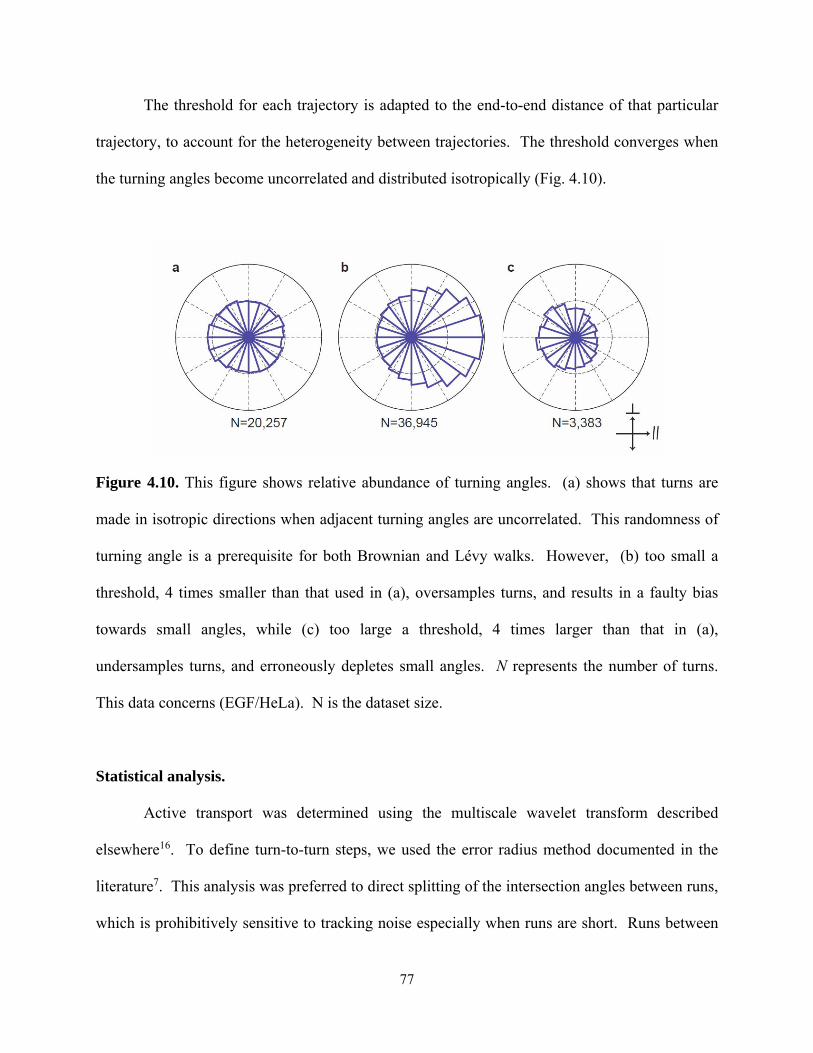
77  

The threshold for each trajectory is adapted to the end-to-end distance of that particular

trajectory, to account for the heterogeneity between trajectories. The threshold converges when

the turning angles become uncorrelated and distributed isotropically (Fig. 4.10).

Figure 4.10. This figure shows relative abundance of turning angles. (a) shows that turns are

made in isotropic directions when adjacent turning angles are uncorrelated. This randomness of

turning angle is a prerequisite for both Brownian and Lévy walks. However, (b) too small a

threshold, 4 times smaller than that used in (a), oversamples turns, and results in a faulty bias

towards small angles, while (c) too large a threshold, 4 times larger than that in (a),

undersamples turns, and erroneously depletes small angles. N represents the number of turns.

This data concerns (EGF/HeLa). N is the dataset size.

Statistical analysis.

Active transport was determined using the multiscale wavelet transform described

elsewhere16. To define turn-to-turn steps, we used the error radius method documented in the

literature7. This analysis was preferred to direct splitting of the intersection angles between runs,

which is prohibitively sensitive to tracking noise especially when runs are short. Runs between

78  

two consecutive turning points are defined as persistent and they are lumped together for

measure of turn-to-turn flight lengths. The relative abundance of persistent, turning, and motion

that reverses directions (“tug-of-war”) was quantified (Fig. 4.7). However, as tug-of-war events

do not change the overall angle of the transport, we excluded them from subsequent analysis.

To calculate the run length and flight length distributions, we used equal number of data

points per bin instead of equal distance per bin which is known to give larger statistical errors in

the tail because of the much smaller counts per bin in the tail. This binning method has been

shown to reproduce the actual shape of distribution while avoiding large uncertainty in fitting the

tail. To distinguish exponential, stretched exponential, and power-law distributions, model

selection was carried out following the standard literature method, Akaike Information

Criterion25. Briefly, the log-likelihood functions for each model were computed as described in

the literature with range of the tails (>2.9 µm) determined by the goodness-of-fit tests; and then

the relative likelihoods were used as weights of evidence in favor of each model (Akaike

weights). As likelihood functions scale exponentially with the number of data points, with our

datasets that typically contain 16,000-60,000 runs and 3,000-11,000 flights for each experimental

condition, Akaike weights can approach 1 for the model that is dominantly favored. This has

allowed unambiguous selection of the more likely model.

Numerical simulations.

We consider a cargo is transported against a constant external opposing force F along a

microtubule with n motors available for binding. At time t, n (0<n≤n ) motors are engaged,

sharing the load /F n . The unbinding rate for an engaged motor to dissociate from the

microtubule is load-dependent, 0 exp / dn n F nF , where 0 is the zero-load unbinding

79  

rate and dF is the detachment force. The binding rate is 0n n n , as it is limited by the

number of available unbound motors ( n -n) and 0 is the binding constant for single motor.

The trajectories are generated by the Gillespie algorithm. Briefly, at 0t , n is randomly

selected from a discrete uniform distribution in the interval max1, N , where maxN is the

maximum number of motors that can be possibly available. This number should be physically

bound by the maximum density of the motors attached to the cargo surface, and depends on the

cargo size and the surface area that is close to microtubule26. At each time step, with probability

( )n

pn n

, an available motor may bind; otherwise, an engaged motor unbinds. Then

time advances by a random number t drawn from an exponential distribution function with a

mean of

1

n n . If s

FF

n ( sF is stall force), the cargo moves by v t , assuming a

constant velocity v ; if not, the transport pauses. If n drops to zero, a “flight” ends, the transport

turns with a random angle, and a new N is assigned. A “flight” also ends if the length exceeds

the limit (100 µm) representing the size of a cell. We found that the numerical results are

insensitive to the length limit used. This physical process generates numerically length

distribution functions, which have shapes determined by a set of dimensionless parameters, d

F

F,

0

0

, s

F

F, and maxN (Fig. 4.8). Among these parameters,

s

F

F only contributes to the run length

distribution without affecting the flight length distribution. To compare with experiments,

simulated trajectories are mapped to experimental length scale by tuning the length unit, 0

(Table 1). 1,000,000 flights were simulated for each parameter set.

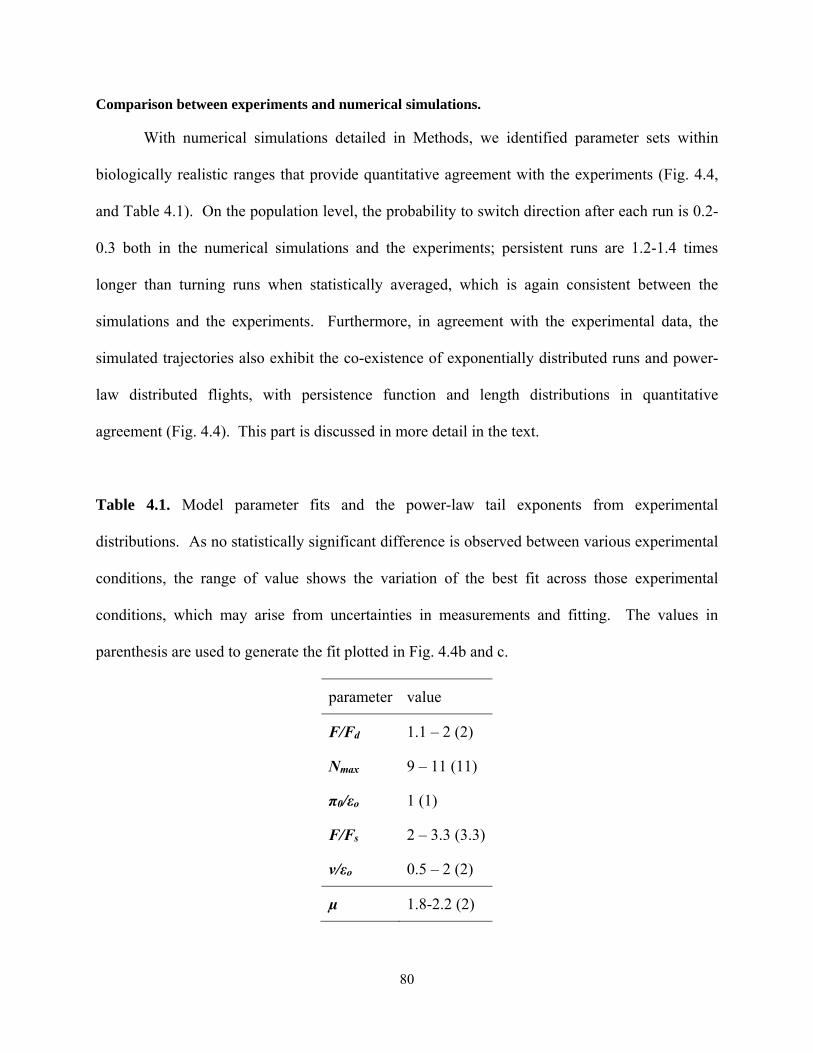
80  

Comparison between experiments and numerical simulations.

With numerical simulations detailed in Methods, we identified parameter sets within

biologically realistic ranges that provide quantitative agreement with the experiments (Fig. 4.4,

and Table 4.1). On the population level, the probability to switch direction after each run is 0.2-

0.3 both in the numerical simulations and the experiments; persistent runs are 1.2-1.4 times

longer than turning runs when statistically averaged, which is again consistent between the

simulations and the experiments. Furthermore, in agreement with the experimental data, the

simulated trajectories also exhibit the co-existence of exponentially distributed runs and power-

law distributed flights, with persistence function and length distributions in quantitative

agreement (Fig. 4.4). This part is discussed in more detail in the text.

Table 4.1. Model parameter fits and the power-law tail exponents from experimental

distributions. As no statistically significant difference is observed between various experimental

conditions, the range of value shows the variation of the best fit across those experimental

conditions, which may arise from uncertainties in measurements and fitting. The values in

parenthesis are used to generate the fit plotted in Fig. 4.4b and c.

parameter value

F/Fd 1.1 – 2 (2)

Nmax 9 – 11 (11)

π0/εo 1 (1)

F/Fs 2 – 3.3 (3.3)

ν/εo 0.5 – 2 (2)

µ 1.8-2.2 (2)

81  

4.5 References

1. Shlesinger, M.F., Zaslavsky, G.M. & Klafter, J. Strange kinetics. Nature 363, 31-37 (1993).

2. Peterson, J., Dixit, P.D. & Dill, K.A. A maximum entropy framework for nonexponential

distributions. Proceedings of the National Academy of Sciences of the United States of America

110, 20380-20385 (2013).

3. Bouchaud, J.P. & Georges, A. Anomalous diffusion in disordered media - statistical mechanisms,

models and physical applications. Physics Reports-Review Section of Physics Letters 195, 127-

293 (1990).

4. Bao, G. & Suresh, S. Cell and molecular mechanics of biological materials. Nature Materials 2,

715-725 (2003).

5. Loverdo, C., Benichou, O., Moreau, M. & Voituriez, R. Enhanced reaction kinetics in biological

cells. Nature Physics 4, 134-137 (2008).

6. Wang, B., Kuo, J. & Granick, S. Bursts of active transport in living cells. Physical Review Letters

111 (2013).

7. Trong, P.K., Guck, J. & Goldstein, R.E. Coupling of active motion and advection shapes

intracellular cargo transport. Physical Review Letters 109 (2012).

8. Brangwynne, C.P., Koenderink, G.H., MacKintosh, F.C. & Weitz, D.A. Intracellular transport by

active diffusion. Trends in Cell Biology 19, 423-427 (2009).

9. Mueller, M.J.I., Klumpp, S. & Lipowsky, R. Tug-of-war as a cooperative mechanism for

bidirectional cargo transport by molecular motors. Proceedings of the National Academy of

Sciences of the United States of America 105, 4609-4614 (2008).

10. Klumpp, S. & Lipowsky, R. Cooperative cargo transport by several molecular motors.

Proceedings of the National Academy of Sciences of the United States of America 102 (2005).

11. Howard, J. Mechanical signaling in networks of motor and cytoskeletal proteins. Annual Review

of Biophysics 38, 217-234 (2009).

82  

12. Huet, S. et al. Analysis of transient behavior in complex trajectories: Application to secretory

vesicle dynamics. Biophysical Journal 91 (2006).

13. Arcizet, D., Meier, B., Sackmann, E., Raedler, J.O. & Heinrich, D. Temporal analysis of active

and passive transport in living cells. Phys. Rev. Lett. 101 (2008).

14. Bressloff, P.C. & Newby, J.M. Stochastic models of intracellular transport. Reviews of Modern

Physics 85, 135-196 (2013).

15. Reilein, A., Yamada, S. & Nelson, W.J. Self-organization of an acentrosomal microtubule

network at the basal cortex of polarized epithelial cells. Journal of Cell Biology 171, 845-855

(2005).

16. Chen, K., Wang, B., Guan, J. & Granick, S. Diagnosing heterogeneous dynamics in single-

molecule/particle trajectories with multiscale wavelets. Acs Nano 7, 8634-8644 (2013).

17. Fakhri, N. et al. High-resolution mapping of intracellular fluctuations using carbon nanotubes.

Science (New York, N.Y.) 344, 1031-1035 (2014).

18. Tabei, S.M.A. et al. Intracellular transport of insulin granules is a subordinated random walk.

Proceedings of the National Academy of Sciences of the United States of America 110, 4911-4916

(2013).

19. Balint, S., Verdeny Vilanova, I., Sandoval Alvarez, A. & Lakadamyali, M. Correlative live-cell

and superresolution microscopy reveals cargo transport dynamics at microtubule intersections.

Proceedings of the National Academy of Sciences of the United States of America 110, 3375-3380

(2013).

20. Ross, J.L., Ali, M.Y. & Warshaw, D.M. Cargo transport: molecular motors navigate a complex

cytoskeleton. Current Opinion in Cell Biology 20, 41-47 (2008).

21. Bartumeus, F., Peters, F., Pueyo, S., Marrase, C. & Catalan, J. Helical Levy walks: Adjusting

searching statistics to resource availability in microzooplankton. Proceedings of the National

Academy of Sciences of the United States of America 100, 12771-12775 (2003).

83  

22. de Jager, M., Weissing, F.J., Herman, P.M.J., Nolet, B.A. & van de Koppel, J. Levy walks evolve

through interaction between movement and environmental complexity. Science 332, 1551-1553

(2011).

23. Viswanathan, G.M. et al. Optimizing the success of random searches. Nature 401, 911-914

(1999).

24. Palyulin, V.V., Chechkin, A.V. & Metzler, R. Lévy flights do not always optimize random blind

search for sparse targets. Proceedings of the National Academy of Sciences 111, 2931-2936

(2014).

25. Edwards, A.M. et al. Revisiting Levy flight search patterns of wandering albatrosses, bumblebees

and deer. Nature 449, 1044-U1045 (2007).

26. Herold, C., Leduc, C., Stock, R., Diez, S. & Schwille, P. Long-range transport of giant vesicles

along microtubule networks. Chemphyschem 13, 1001-1006 (2012).

27. Anthony, S.M. & Granick, S. Image analysis with rapid and accurate two-dimensional gaussian

fitting. Langmuir 25, 8152-8160 (2009).

28. Anthony, S., Zhang, L.F. & Granick, S. Methods to track single-molecule trajectories. Langmuir

22, 5266-5272 (2006).

29. Turchin, P. Quantitative analysis of movement: measuring and modeling population redistribution

in animals and plants. (Sinauer Associates, Incorporated, 1998).

84  

CHAPTER 5

INTERMITTENT MOTION OF SEMI-FLEXIBLE

POLYMERS IN NETWORK

5.1 Background

Brownian motion is a fundamental phenomenon that continues to fascinate researchers.

While diffusion of spherical objects has been well understood, recent studies show that shape of

a diffusing object adds additional complexity to transport dynamics.1, 2 An unexplored aspect in

transport dynamics is when shape is flexible and fluctuates spontaneously. Little was known

about the relevance of shape fluctuations because most previous research focused on center-of-

mass dynamics without visualizing shape or lacked a feasible way to analyze shape fluctuations

especially in relation to transport dynamics. Here, we demonstrate a strong coupling between

shape fluctuation of polymer chain and its transport in networks at equilibrium with direct

imaging of single DNA chains. We chose DNA chains because they are big enough for shape

visualization in real time and flexible enough to show spontaneous shape fluctuations. Shape

information is extracted from images with description at various levels of details from pixel-

based multi-dimension to coarse-grained one-dimension and correlated with the center of mass

motion. The prevailing pattern is that the shape and motion of the chains are simultaneously

arrested most of the time and spontaneous large chain extension or retraction transiently allows a

                                                              The contents of this chapter are based on experiments done by Bo Wang, Juan Guan, James Kuo, and

Ah-Young Jee.

85  

chain to break free and achieve net transport. Tracking chain ends reveals that blocked end

motion is consistent with the arrest of shape and chain motion. This novel mode of transport

might be important to transport in porous media and crowded environment as shape fluctuation is

widely present in a broad class of soft materials.

5.2 Results and Discussions

We embed -DNA chains uniformly labeled with fluorescence dyes in optically

transparent network as sketched schematically in Fig. 5.1a. Network concentration is tuned such

that a chain (~16 μm in contour length; ~50 nm in persistence length) threads through ~20-40

meshes (~200 nm) to be tightly entangled with the network (materials and methods). The large

size of -DNA allows shape imaging (much exceeding diffraction limit ~0.3 μm). To test the

generality of the finding, two types of network with matching mesh size are chosen: agarose

hydrogel and semidilute solution of actin filaments. The former represents static network as

crosslinked agarose fibers form interconnected meshes whereas the latter represents dynamic

network as actin filaments fluctuate and rearrange locally over observation time window.3, 4

86  

Figure 5.1. Intermittent dynamics of shape, center-of-mass and ends for chains embedded in

networks. a) Schematic of a λ-DNA chain (~16 μm in length) embedded in agarose or actin

networks (~200 nm mesh size). The open space in the network is filled with water. The

magnified view shows schematically flexible turns and bends of chain segments within one mesh.

b) (top) Similarity matrix calculates pixel-based correlation between pairwise images for a chain

with each element indicating how similar two images are. Examples for both networks are

shown. Both axes of the matrix denote time in seconds. Red blocks indicate high similarity

between two images whereas blue blocks indicate low similarity. A color bar is shown for

comparison. (bottom) Center-of-mass position for the corresponding chains. Top and bottom

panels share the time axis. Details see main text. c) Position versus time for two ends of one

chain. The two ends are often confined in different meshes microns apart.

DNA chains adopt diverse shapes in these networks, from collapsed globule to extended

chains with many twists and turns. Unexpectedly, in both networks the chains can keep a

87  

relatively constant shape for extended periods of time. This arrested shape dynamics is very well

captured by the similarity matrix S (Fig. 5.1b), with S(m,n) calculated as the pixel-based

correlation between frame m and n in the time series of images of one specific chain and

indicates how similar these two images are. Fig. 5.1b shows the shape matrices of two 62 s long

movies from both networks, with red and blue representing high and low similarity respectively.

Evident to the eye, the matrices are composed of blocks with different color and size. Along the

diagonal line, transition from one square to the next corresponds to large change in chain

position as seen from the steep slope in the position of center-of-mass plot below the matrices.

The fact that the diagonal squares are mostly red indicates that the shape and position of a chain

remains mostly constant within each square. The arrest of shape and chain position is really

surprising because it is commonly assumed that flexible polymers in network smoothly and

continuously slither back and forth in “tubes” formed by its surrounding obstacles.5, 6 A key

assumption in this reptation picture is that the chain ends can freely explore the network.7, 8 To

test this assumption, we fluorescently labeled just the chain ends9 and find that they are locally

confined on a length scale comparable to mesh size with occasional hops (Fig. 5.1c) (materials

and methods about ends labeling). Furthermore, the two ends seem to move and pause at

different times, independent to one another. The distance between ends fluctuates at around 5

mesh size and two ends often stay in different meshes microns apart, confirming the tightly

entangled regime where a chain threads through many meshes. Given the blocked ends motion

and transverse confinement along the chain contour, it is reasonable to expect shape and position

arrest. We note that the blocked ends motion is not an artifact from projection of vertical motion

as the depth of focus is only ~1 μm and out-of-focus images are easily discerned and excluded

from analysis.

88  

Figure 5.2. Coupling between shape fluctuation and chain motion. a) Sequential images taken

from a typical center-of-mass hop, as highlighted with a red arrow in Fig. 5.1b. The initial

center-of-mass position is overlaid for comparison (+). The chain extension is accompanied by

position hop. Image size is 2.9 μm×1.5 μm. b) Chain position hop and chain length fluctuation

occur simultaneously; position arrest and shape arrest occur simultaneously. Hundreds of

individual traces are shown. Red curve denotes average. c) Mean squared displacement (MSD)

during hops than arrest. The hops are identified from ~1,000,000 images using a wavelet method.

Solid curves are for agarose and dashed curves are for actin network. d) Average apparent (L)

change (∆ √ ∆ ) during hops is larger and faster than during arrest. Symbols are the

same as in c.

89  

It is clear from the similarity matrix and the center-of-mass motion that arrested

dynamics dominates in time and only the occasional swift hops are responsible for the transport

of the chains. When taking a closer look at hops, we saw that a chain typically shows shape

change during hops, in contrast to almost no shape fluctuations other time (Fig. 5.2a, more

examples in materials and methods). To see how general this pattern is, we used multiscale

wavelet analysis10 to automatically identify the hops across hundreds of chains and then

compared shape fluctuation during these hops versus local motion. The appropriate separation

between hopping and local rattling is confirmed with the distinct fast and slow center-of-mass

dynamics (Fig. 5.2c). Local rattling motion occupies 90% of the time determined by wavelet

analysis. As extension and retraction appear to be the dominant form of chain shape fluctuation,

we use apparent chain length here as a measure of global chain shape (see materials and methods

for apparent chain length estimation). Checking across hundreds of chains, we consistently find

large chain extension or retraction during hops whereas almost no length change is observed

during local rattling (Fig. 5.2b). Other shape indicators are checked in parallel to confirm the

coupling between shape fluctuation and chain motion exists in both networks (materials and

methods). We further compare the ensemble-averaged apparent length change (∆L) with time

during hopping versus local rattling from over ~1,000,000 images. The shape fluctuation during

hopping is significantly faster and larger than local rattling (Fig. 5.2d), confirming that chain

motion is accompanied by chain extension or retraction. Physically, the blocked chain ends can

occasionally hop to other meshes and create entropic tension between the chain segments so the

chain shape changes to release the tension and causes center-of-mass position shift.

90  

Figure 5.3. The kinetics and magnitude of the hops. a) Waiting time between hops follows

stretched exponential distribution with exponent of ~ 0.7. b) Distribution of hop distance for

individual hops. Solid symbols are for agarose and open symbols are for actin network.

The local confined motion suggests transport barriers imposed by the network. The

waiting time distribution can be fitted with stretched exponential with exponent of ~ 0.7 (Fig.

5.3a), suggesting a heterogeneous distribution of barrier height. The hop length has an average

of ~0.25 μm for both networks, comparable to the mesh size (Fig. 5.3b) suggesting that the scale

of discrete hops is determined by the underlying network mesh. This length is comparable to the

hop length of chain ends (materials and methods) further supporting the hops are initiated at

91  

chain ends. It is worth noting that other chains sufficiently long to observe shape (e.g. half -

DNA length) display similar behavior such as intermittent dynamics, coupling between chain

motion and shape fluctuation, and comparable hop length (materials and methods).

5.3 Conclusions

The ensemble-averaged chain dynamics is initially sub-diffusive with a scaling of 0.4 and

0.6 for agarose and actin network respectively and transits to diffusion at ~10 s (materials and

methods). It is commonly assumed that flexible polymers in solution smoothly and continuously

slither back and forth in “tubes” formed by its surrounding obstacles. It is only remarkable now

that direct visualization suggests alternative process involving intermittent dynamics and shape

fluctuations coupled to chain motion. Hindered motion is unlikely to be caused by specific

interactions as we demonstrate in two distinct systems although its exact origin is unknown.

Tentatively, if we consider DNA chain as worm-like-chain with persistence length on the order

of mesh size, it might have trouble wriggling through rigid network meshes (materials and

methods). Taken together the intermittent dynamics of shape, center-of-mass, and chain ends, it

is likely that a chain spanning multiple interconnected meshes hosting different parts of the chain

along its contour experiences an effective confinement. It remains to be tested whether similar

dynamics exists in polymer melt systems where probe chain and surrounding chains are more

flexible. Interesting questions remain on how the phenomenon at equilibrium might transfer to

non-equilibrium dynamics where different microscopic processes compete differently. On the

practical side, the long waiting time observed here might slow down diffusion processes, an

effect less studied in the context of polymer dynamics in networks, for applications in transport,

mixing, and spatial distribution of constituents in networks.

92  

5.4 Materials and Methods

Sample preparations and imaging condition.

-DNA chain (48 kbp in length), covalently labeled with dyes (Mirus Bio) uniformly

along the contour, was embedded in 1.5 wt% agarose gel (Fisher, molecular biology grade, low

EEO) in the presence of 1× TBE and anti-photobleaching buffer, and visualized using a

homebuilt epifluorescence microscope setup (Zeiss observer.Z1, 100× objective with N.A.=1.45)

with time resolution of 12 ms (Andor iXon EMCCD camera) and pixel size of 64 nm.

Determine entanglement regime.

We estimate the entanglement level for -DNA in agarose gel to be ~25, a regime

commonly accessed in simulations and experiments and typically assumed to represent long-

chain condition. First, we estimate the entanglement level based on length scale of the system.

λ-DNA (~16 μm) contains ~160 Kuhn blobs (~0.1 μm). The reported agarose pore size at 1.5%

ranging from 0.1-0.4 μm.11 Taking an intermediate value of 0.25 μm which can contain ~6 Kuhn

blobs per pore (√6 0.1 0.25 ) and therefore the whole chain fits in ~25 pores. The

range of 0.1-0.4 μm gives ~10-160 pores. Next, the two ends of a chain often stay in different

pores indicating the mass is distributed in multiple pores network – otherwise the two ends

should often co-localize to the same pore if a chain on average occupied one single big pore.

Based on the measured end-to-end distance of ~1.5 μm and reported pore size, the chain is

distributed in ~14-225 pores, consistent with earlier estimate. Therefore, the effective cage

experienced by a chain, rather than corresponding to one single pore of the network, is likely

spanning multiple interconnected pores hosting different parts of a chain. Third, we apply the

93  

same calculation to an artificial 2D array of ~0.92-μm pores for comparison. λ-DNA was found

to mostly distribute to two pores. One pore can contain ~80 Kuhn blobs (√80 0.1

0.9 ), consistent with the current experiments.

On similarity matrix.

To go beyond center-of-mass dynamics, we calculate correlation between any two images

of a chain to construct “similarity matrix.” Both axes of the matrix represent time. The value of

each element is the correlation coefficient between a pair of images from a time series of images.

By definition, the matrix is symmetric and the value of diagonal elements is 1. High value (red)

indicates high similarity between the two images whereas low (blue) value indicates low

similarity. Here, both position shift and shape fluctuation can be sensitively detected as change

in similarity.

Analyze patterns on similarity matrix.

The “success” and “futile” processes described in main text correspond to different

patterns on the similarity matrix: “success” corresponds to the intersection between diagonal

blocks (Fig. 5.2b and 4) where the correlation between images before and after transition is

extremely low (close to 0) as shown in off-diagonal blue blocks; “futile” corresponds to the

stripe within a diagonal block (Fig. 5.2b and 4) where intermediate correlation is seen as a chain

never fully leaves its initial position (i.e. stripes are typically yellow or green).

94  

Figure 5.4. The initial center-of-mass position is overlaid for comparison (+). In 2, the

molecule stretches and recoils to a new position. In 3, the molecule stretches but never fully

leaves its original position. The durations of the events are 0.20 s and 0.25 s, respectively. Image

size is 2.2 μm×1.7 μm.

To identify the block pattern and the stripes within the block, we perform PCA analysis

on the similarity matrix and the coefficient of the first principal component contains the

information about the locations of blocks and stripes as shown in Fig. 5.5. We manually check

and correct for misidentified features after PCA analysis to ensure accuracy.

95  

Figure 5.5. The block and stripe patterns of the similarity matrix can be identified from PCA

analysis. Top row shows two similarity matrices. The bottom row shows the corresponding

coefficient of the first principal component. The block and stripe features of the matrix are

reflected on the coefficients. The sign change between positive and negative values marks the

boundary of blocks, denoted by black dots on the matrix. The local peaks of coefficients

correspond to stripe features, denoted by white dots on the matrix.

To analyze separately jumping and caging states, we first identify the edges of the blocks

and stripes and include neighboring frames within 0.37 s as jumping states, and the ensemble

excluding jumping are categorized as caging. Time interval of 0.37 s is empirically determined

as most transient transitions last less than 0.37 s. Using different parameters of time intervals

does not change the distinct dynamics and shape fluctuation we see (Fig. 5.6, top). Including

96  

only “success” (block features) as jumping states does not change the conclusion either (Fig. 5.6,

bottom).

Figure 5.6. The difference between jumping and caging is robustly seen across a range of

parameter choices. Panel a and b compare jumping states of duration 0.37 s (line) and 0.25 s (○).

Panel c and d compare jumping states including all jumps (○) versus only “success” jumps (line).

Caging is dominant, accounting for ~94% of the images. The “success” and “futile”

correspond to 2% and 4% of the time (Fig. 5.7).

97  

Figure 5.7. Caging is dominant, accounting for ~94% of the time. The “success” and “futile”

correspond to 2% and 4% of the time.

To calculate jump distance, we calculate the distance between mean caging positions

between blocks for “success” jumps and the distance between mean position on a stripe and

mean position of the block containing the stripe for “futile” jumps.

Block feature of the similarity matrix is unique to caging and intermittent dynamics.

A few representative similarity matrices are shown in Fig. 5.8 for comparison. Block

feature is absent.

98  

Figure 5.8. (top) similarity matrices in the case of free diffusion of λ-DNA in sucrose. (bottom)

similarity matrices for simulated Brownian diffusion of λ-DNA in dilution solution.

Figure 5.9. Two representative fluorescence images overlaid with circles with a radius of .

The image size is 2.5 μm×2.5 μm.

99  

Shape fluctuation measured with from fluorescence images.

Radius of gyration ( ) is a robust measure of chain size. ∑ . .

. ./ where . . and . . are center-of-mass positions, and are

coordinates of pixels with intensity . See examples in Fig. 5.9. The current system reports a

smaller value for λ-DNA compared to previous studies elsewhere.12 The difference mainly

comes from two aspects: a) this current system uses a covalent dye labeling method that does not

extend the chain whereas previous systems use intercalating dyes that extends the chain contour

length from 16 μm to 22 μm; b) this system uses high salt concentration (~200 mM monovalent

salt) whereas previous systems typically have ~10 mM salt. To quantify shape fluctuation,

∆ ∆ is calculated where T is sampled

across jumping states, caging states, and ensemble for averaging over all trajectories.

In principle, other shape indicators are sufficient to characterize the shape fluctuations as

well, such as long and short axis of , or line-tracking.13 We choose because its physical

meaning is a common quantity to measure chain size in polymer physics context.

Conventional theories of contour length fluctuation (CLF) predicts the amplitude of

fluctuation on the order of end-to-end distance (~1 μm), which would be reflected as ~3% in

change since 16 μm and ~√ .

100  

Theoretical timescale estimation under reptation framework.

The experimental system shows that the mean squared displacement of center-of-mass of

-DNA transits from sub-diffusion (with a scaling of ½) to diffusion (scaling of 1). Although

consistent with reptation prediction, the direct observation of microscopic process suggests an

alternative explanation.

In reptation picture, the thermal motion of center-of-mass has a scaling exponent of ½

before reptation time because it is a random walk within a tube of random walk configuration.

The dynamics transit to diffusion with a scaling exponent of 1 beyond reptation time.

The reptation time is estimated to be ~16 s for this system. Each entanglement blob has a

relaxation timescale of 2 ms assuming the size of each blob ( ) is 0.2 μm, close to pore size of

the network ( 2 ). Reptation time 16 assuming a chain

contains ~20 entanglement blobs.

Experimental uncertainty in determining center-of-mass position.

A range of intensity threshold is set to identify features in fluorescence images. With a

pixel size of 64 nm, λ-DNA typically shows up as a feature occupying over 100 pixels, showing

shape exceeding the diffraction limit (Fig. 5.2a and 9). Varying the threshold gives <10 nm

variation in center-of-mass position, which is calculated according to intensity-weighted average

. .∑

∑.

101  

The size of chain ends are below the diffraction limit and determined by fitting a 2D

Gaussian intensity profile with uncertainty <30 nm.

Shorter chains display similar intermittent dynamics and transient shape fluctuations

during jumps.

Chains of 23 kbp, about half the λ-DNA length, is sufficiently big for visualizing shape.

Fig. 5.10 shows similarity matrix for a representative chain. The block pattern is similar to the λ-

DNA system showing caging and intermittent dynamics. Fig. 5.11 shows snapshots from a

jumping event where transient stretch and recoil is coupled to chain motion.

Figure 5.10. On the left is a representative center-of-mass trajectory of 23 kbp in gel.

Trajectory lasts ~50 s. The corresponding similarity matrix is shown on the right. Three

diagonal blocks reflects three main cages in the trajectory.

102  

Figure 5.11. Sequential images from a representative jumping event for a DNA chain of 23 kbp

in gel. The first three snapshots show a “futile” process and the last two snapshots show the

subsequent “success” process. The duration of the event is 1 s. Image size is 2 μm×1.3 μm.

5.5 References

1. Chakrabarty, A. et al. Brownian Motion of Arbitrarily Shaped Particles in Two Dimensions.

Langmuir 30, 13844-13853 (2014).

2. Han, Y. et al. Brownian motion of an ellipsoid. Science 314, 626-630 (2006).

3. Kas, J., Strey, H. & Sackmann, E. Direct Imaging Of Reptation For Semiflexible Actin-Filaments.

Nature 368, 226-229 (1994).

4. Glaser, J. et al. Tube Width Fluctuations in F-Actin Solutions. Physical Review Letters 105

(2010).

5. Perkins, T.T., Smith, D.E. & Chu, S. Direct observation of tube-like motion of a single polymer-

chain. Science 264, 819-822 (1994).

6. Milner, S.T. & McLeish, T.C.B. Reptation and contour-length fluctuations in melts of linear

polymers. Physical Review Letters 81, 725-728 (1998).

7. Wischnewski, A., Monkenbusch, M., Willner, L., Richter, D. & Kali, G. Direct observation of the

transition from free to constrained single-segment motion in entangled polymer melts. Physical

Review Letters 90 (2003).

8. Hou, J.-X., Svaneborg, C., Everaers, R. & Grest, G.S. Stress Relaxation in Entangled Polymer

Melts. Physical Review Letters 105 (2010).

103  

9. Guan, J., Wang, B., Bae, S.C. & Granick, S. Modular stitching to image single-molecule DNA

transport. Journal of the American Chemical Society 135, 6006-6009 (2013).

10. Chen, K., Wang, B., Guan, J. & Granick, S. Diagnosing Heterogeneous Dynamics in Single-

Molecule/Particle Trajectories with Multiscale Wavelets. Acs Nano 7, 8634-8644 (2013).

11. Fakhri, N. et al. High-resolution mapping of intracellular fluctuations using carbon nanotubes.

Science (New York, N.Y.) 344, 1031-1035 (2014).

12. Everaers, R. et al. Rheology and microscopic topology of entangled polymeric liquids. Science

303, 823-826 (2004).

13. Guan, J., Wang, B. & Granick, S. Automated Single-Molecule Imaging To Track DNA Shape.

Langmuir 27, 6149-6154 (2011).