zint1001 - engineering computational tools - part c - engineering applications
TRANSCRIPT

8/4/2019 ZINT1001 - Engineering Computational Tools - Part C - Engineering Applications
http://slidepdf.com/reader/full/zint1001-engineering-computational-tools-part-c-engineering-applications 1/47
Engineering Applications
By
Dr Murat Tahtalı

8/4/2019 ZINT1001 - Engineering Computational Tools - Part C - Engineering Applications
http://slidepdf.com/reader/full/zint1001-engineering-computational-tools-part-c-engineering-applications 2/47
Application to Statics
• If you recall from Statics, solving a trussproblem is a quite onerous task.
• It involves the repetitive solution member
forces and reactions.• In fact, the problem is merely the solution of
N-equations for N-unknowns.
• The brand of application to solve this typeproblems, and more, is called Finite ElementAnalysis (FEA).
UNSW@ADFASEIT & PEMS, S2, 2010
Dr Murat Tahtalı & Dr Isaac Towers 2
8/4/2019 ZINT1001 - Engineering Computational Tools - Part C - Engineering Applications
http://slidepdf.com/reader/full/zint1001-engineering-computational-tools-part-c-engineering-applications 3/47
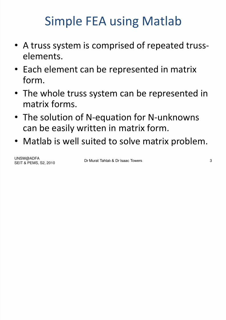
Simple FEA using Matlab
• A truss system is comprised of repeated truss-elements.
• Each element can be represented in matrix
form.• The whole truss system can be represented in
matrix forms.
• The solution of N-equation for N-unknownscan be easily written in matrix form.
• Matlab is well suited to solve matrix problem.
UNSW@ADFASEIT & PEMS, S2, 2010
Dr Murat Tahtalı & Dr Isaac Towers 3
8/4/2019 ZINT1001 - Engineering Computational Tools - Part C - Engineering Applications
http://slidepdf.com/reader/full/zint1001-engineering-computational-tools-part-c-engineering-applications 4/47
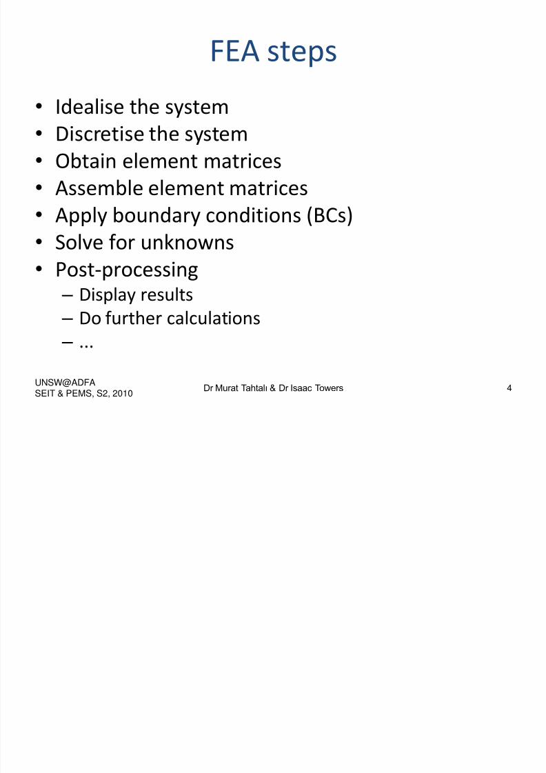
FEA steps
• Idealise the system
• Discretise the system
• Obtain element matrices
• Assemble element matrices• Apply boundary conditions (BCs)
• Solve for unknowns
• Post-processing – Display results
– Do further calculations
– ...
UNSW@ADFASEIT & PEMS, S2, 2010
Dr Murat Tahtalı & Dr Isaac Towers 4
8/4/2019 ZINT1001 - Engineering Computational Tools - Part C - Engineering Applications
http://slidepdf.com/reader/full/zint1001-engineering-computational-tools-part-c-engineering-applications 5/47
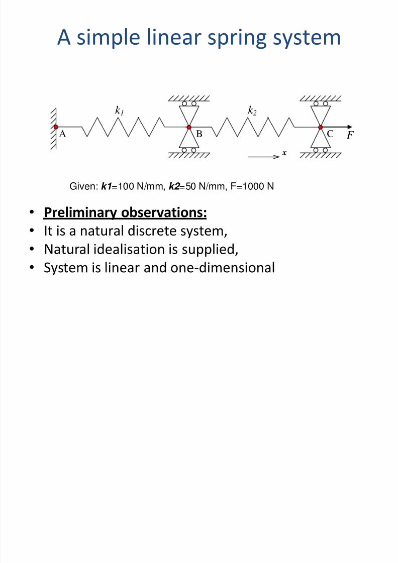
A simple linear spring system
k 2 k 1
F A C B
Given: k1=100 N/mm, k2 =50 N/mm, F=1000 N
• Preliminary observations:• It is a natural discrete system,
• Natural idealisation is supplied,
• System is linear and one-dimensional
8/4/2019 ZINT1001 - Engineering Computational Tools - Part C - Engineering Applications
http://slidepdf.com/reader/full/zint1001-engineering-computational-tools-part-c-engineering-applications 6/47
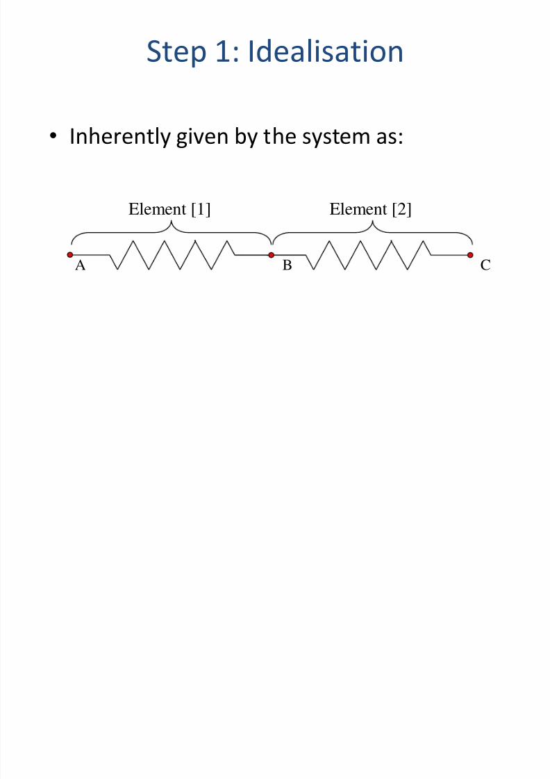
Step 1: Idealisation
• Inherently given by the system as:
A CB
Element [1] Element [2]
8/4/2019 ZINT1001 - Engineering Computational Tools - Part C - Engineering Applications
http://slidepdf.com/reader/full/zint1001-engineering-computational-tools-part-c-engineering-applications 7/47
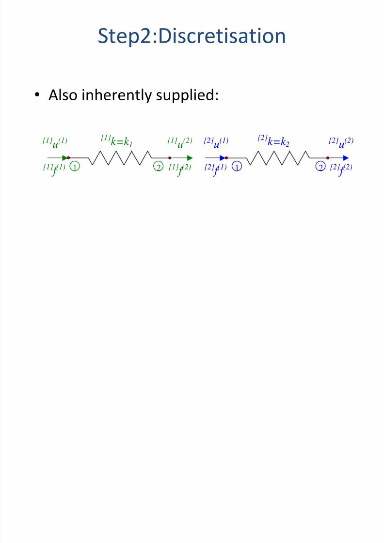
Step2:Discretisation
• Also inherently supplied:
1 2 [1] f (2)[1] f (1)
[1]u(1) [1]u(2)
[2] f (2)[2] f (1)
[2]u(1) [2]u(2)
1 2
[1]k=k 1[2]k=k 2
8/4/2019 ZINT1001 - Engineering Computational Tools - Part C - Engineering Applications
http://slidepdf.com/reader/full/zint1001-engineering-computational-tools-part-c-engineering-applications 8/47
8/4/2019 ZINT1001 - Engineering Computational Tools - Part C - Engineering Applications
http://slidepdf.com/reader/full/zint1001-engineering-computational-tools-part-c-engineering-applications 9/47
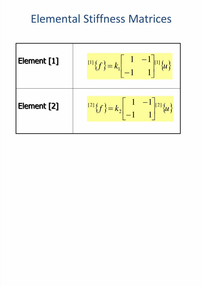
Elemental Stiffness Matrices
Element [1]
Element [2]
uk f
]1[
1
]1[
11
11
uk f ]2[2
]2[
1111

8/4/2019 ZINT1001 - Engineering Computational Tools - Part C - Engineering Applications
http://slidepdf.com/reader/full/zint1001-engineering-computational-tools-part-c-engineering-applications 10/47
8/4/2019 ZINT1001 - Engineering Computational Tools - Part C - Engineering Applications
http://slidepdf.com/reader/full/zint1001-engineering-computational-tools-part-c-engineering-applications 11/47
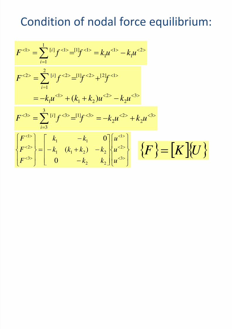
Condition of nodal force equilibrium:
2
1
1
1
1]1[1
1
1][1 uk uk f f F i
i
3
2
2
21
1
1
1]2[2]1[2
1
2][2
)( uk uk k uk
f f f F i
i
3
2
2
2
3]1[3
3
3][3
uk uk f f F i
i
3
2
1
22
2211
11
3
2
1
0
)(
0
u
u
u
k k
k k k k
k k
F
F
F
U K F
8/4/2019 ZINT1001 - Engineering Computational Tools - Part C - Engineering Applications
http://slidepdf.com/reader/full/zint1001-engineering-computational-tools-part-c-engineering-applications 12/47
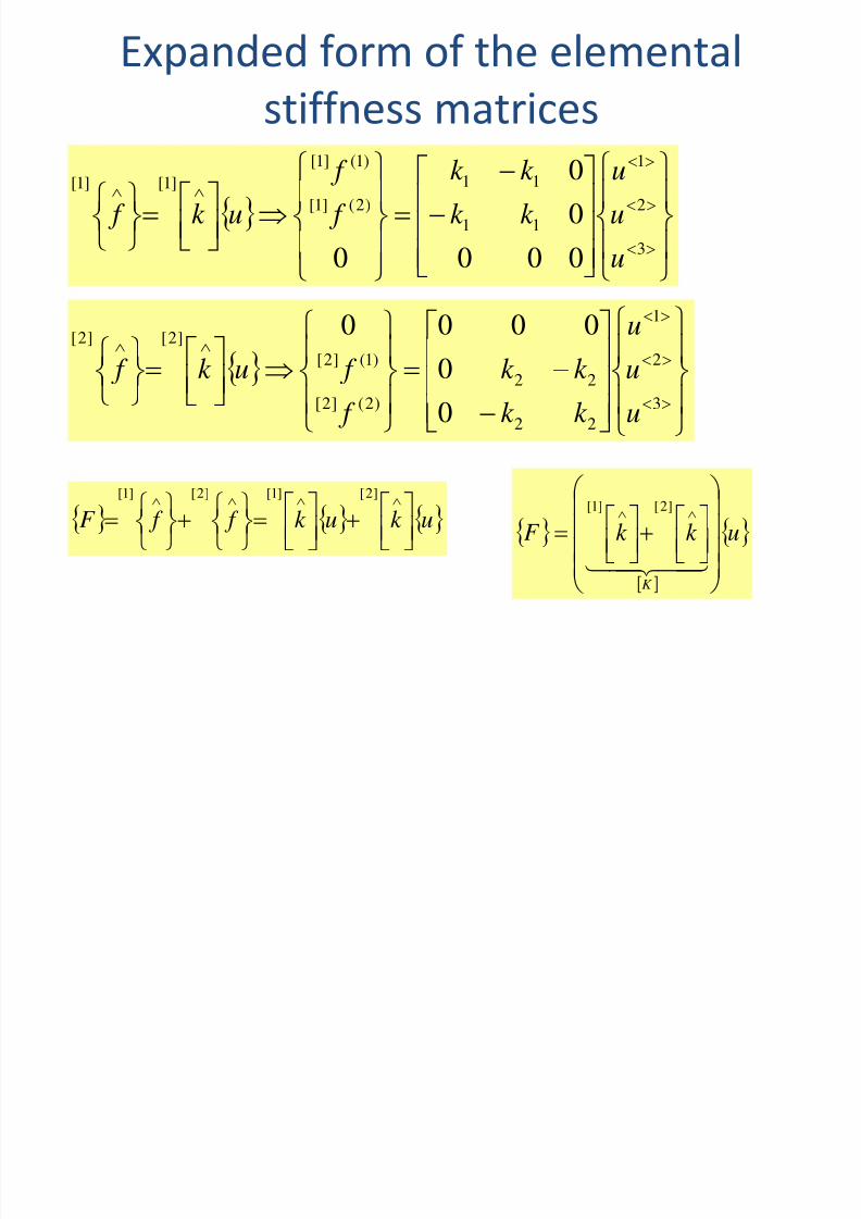
Expanded form of the elemental
stiffness matrices
3
2
1
11
11
)2(]1[
)1(]1[
]1[]1[
000
0
0
0 u
u
u
k k
k k
f
f
uk f
3
2
1
22
22
)2(]2[
)1(]2[
]2[]2[
0
0
0000
u
u
u
k k
k k
f
f uk f
uk uk f f F
]2[]1[]2[]1[
uk k F
K
]2[]1[
8/4/2019 ZINT1001 - Engineering Computational Tools - Part C - Engineering Applications
http://slidepdf.com/reader/full/zint1001-engineering-computational-tools-part-c-engineering-applications 13/47
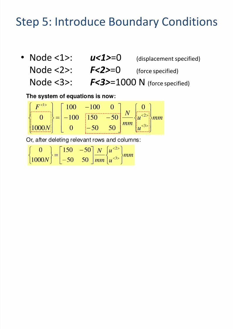
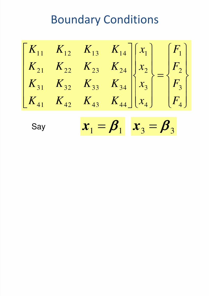
Step 5: Introduce Boundary Conditions
• Node <1>: u<1>=0 (displacement specified)
Node <2>: F<2>=0 (force specified)
Node <3>: F<3>=1000 N (force specified)
The system of equations is now:
mm
u
umm
N
N
F
3
2
1 0
50500
50150100
0100100
1000
0
mm
u
u
mm
N
N
3
2
5050
50150
1000
0
Or, after deleting relevant rows and columns:

8/4/2019 ZINT1001 - Engineering Computational Tools - Part C - Engineering Applications
http://slidepdf.com/reader/full/zint1001-engineering-computational-tools-part-c-engineering-applications 14/47
Step 6: Solve for unknown
displacements
• Solution of the reduced set of equations
yields:
u<2>=10 mm and u<3>=30 mm

8/4/2019 ZINT1001 - Engineering Computational Tools - Part C - Engineering Applications
http://slidepdf.com/reader/full/zint1001-engineering-computational-tools-part-c-engineering-applications 15/47
Step 6: Solve for unknown forces
• F <1>=-1000 N
as it should be in equilibrium

8/4/2019 ZINT1001 - Engineering Computational Tools - Part C - Engineering Applications
http://slidepdf.com/reader/full/zint1001-engineering-computational-tools-part-c-engineering-applications 16/47
Illustrative step-by-step Example
UNSW@ADFASEIT & PEMS, S2, 2010
Dr Murat Tahtalı & Dr Isaac Towers 16
k1 k3
x
<1>
e2
<3>
e1 e3 e4
k2
<2> <4>
k4

8/4/2019 ZINT1001 - Engineering Computational Tools - Part C - Engineering Applications
http://slidepdf.com/reader/full/zint1001-engineering-computational-tools-part-c-engineering-applications 17/47
Interconnectivity Table
Element # Local node # System node #
1 (1) <1>
(2) <2>
2 (1) <1>
(2) <3>
3 (1) <2>
(2) <3>
4 (1) <3>
(2) <4>

8/4/2019 ZINT1001 - Engineering Computational Tools - Part C - Engineering Applications
http://slidepdf.com/reader/full/zint1001-engineering-computational-tools-part-c-engineering-applications 18/47
Element 1
2
1
21
11
111
k k
k k k
4
3
2
1
0000
0000
00
00
11
111
4321
k k
k k
k
1 (1) <1>
(2) <2>

8/4/2019 ZINT1001 - Engineering Computational Tools - Part C - Engineering Applications
http://slidepdf.com/reader/full/zint1001-engineering-computational-tools-part-c-engineering-applications 19/47
Element 2
2 (1) <1>
(2) <3>
3
1
31
22
222
k k
k k k
4
3
2
1
0000
00
0000
00
22
222
4321
k k
k k
k
8/4/2019 ZINT1001 - Engineering Computational Tools - Part C - Engineering Applications
http://slidepdf.com/reader/full/zint1001-engineering-computational-tools-part-c-engineering-applications 20/47
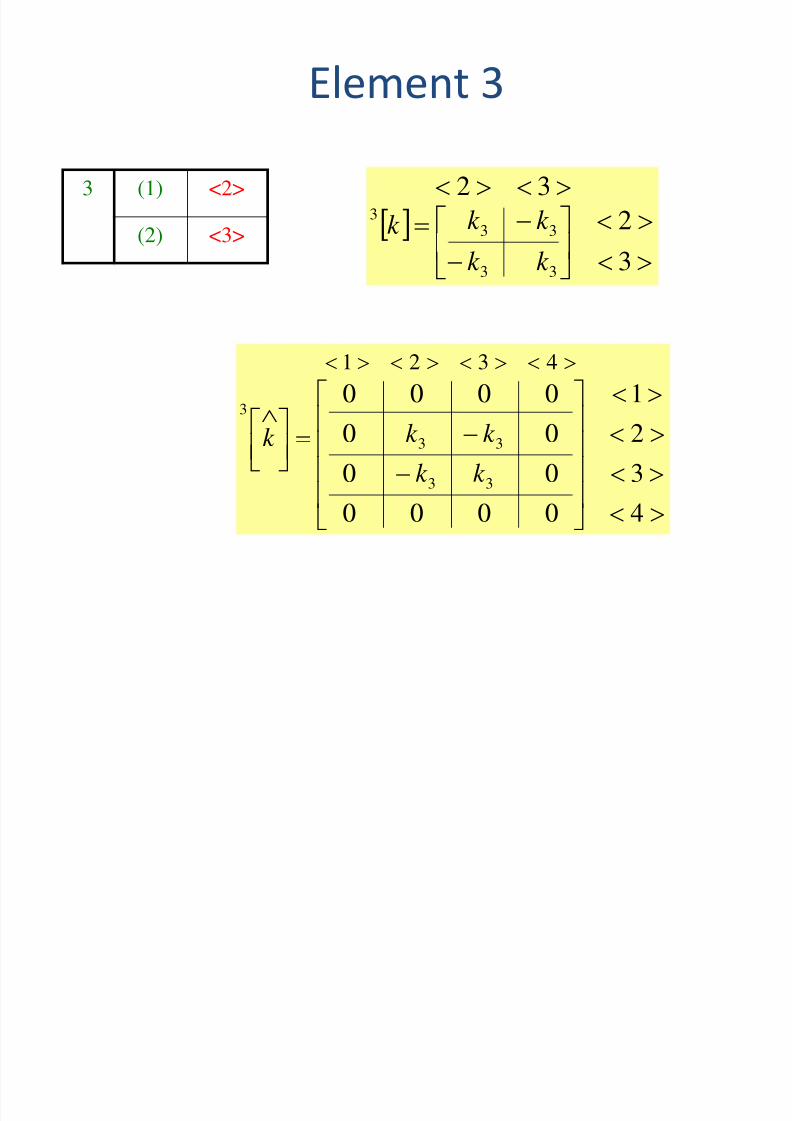
Element 3
3 (1) <2>
(2) <3>
3
2
32
33
333
k k
k k k
4
3
2
1
0000
00
00
0000
33
33
3
4321
k k
k k k
8/4/2019 ZINT1001 - Engineering Computational Tools - Part C - Engineering Applications
http://slidepdf.com/reader/full/zint1001-engineering-computational-tools-part-c-engineering-applications 21/47
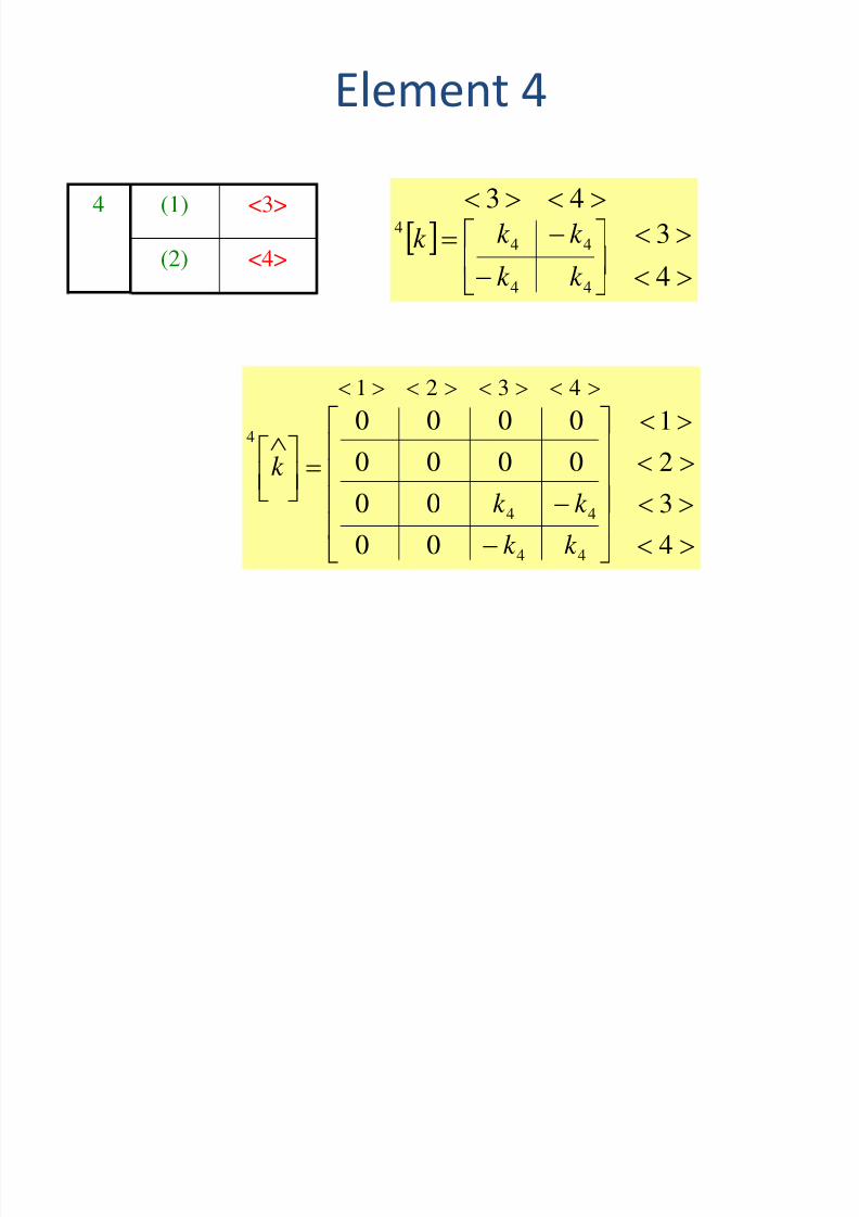
Element 4
4 (1) <3>
(2) <4>
4
3
43
44
444
k k
k k k
4
3
2
1
00
00
0000
0000
44
44
4
4321
k k
k k
k

8/4/2019 ZINT1001 - Engineering Computational Tools - Part C - Engineering Applications
http://slidepdf.com/reader/full/zint1001-engineering-computational-tools-part-c-engineering-applications 22/47
Global Stiffness Matrix
44
443232
3311
2121
4
1
00
0
0
k k
k k k k k k
k k k k
k k k k
k K e
e
8/4/2019 ZINT1001 - Engineering Computational Tools - Part C - Engineering Applications
http://slidepdf.com/reader/full/zint1001-engineering-computational-tools-part-c-engineering-applications 23/47
8/4/2019 ZINT1001 - Engineering Computational Tools - Part C - Engineering Applications
http://slidepdf.com/reader/full/zint1001-engineering-computational-tools-part-c-engineering-applications 24/47
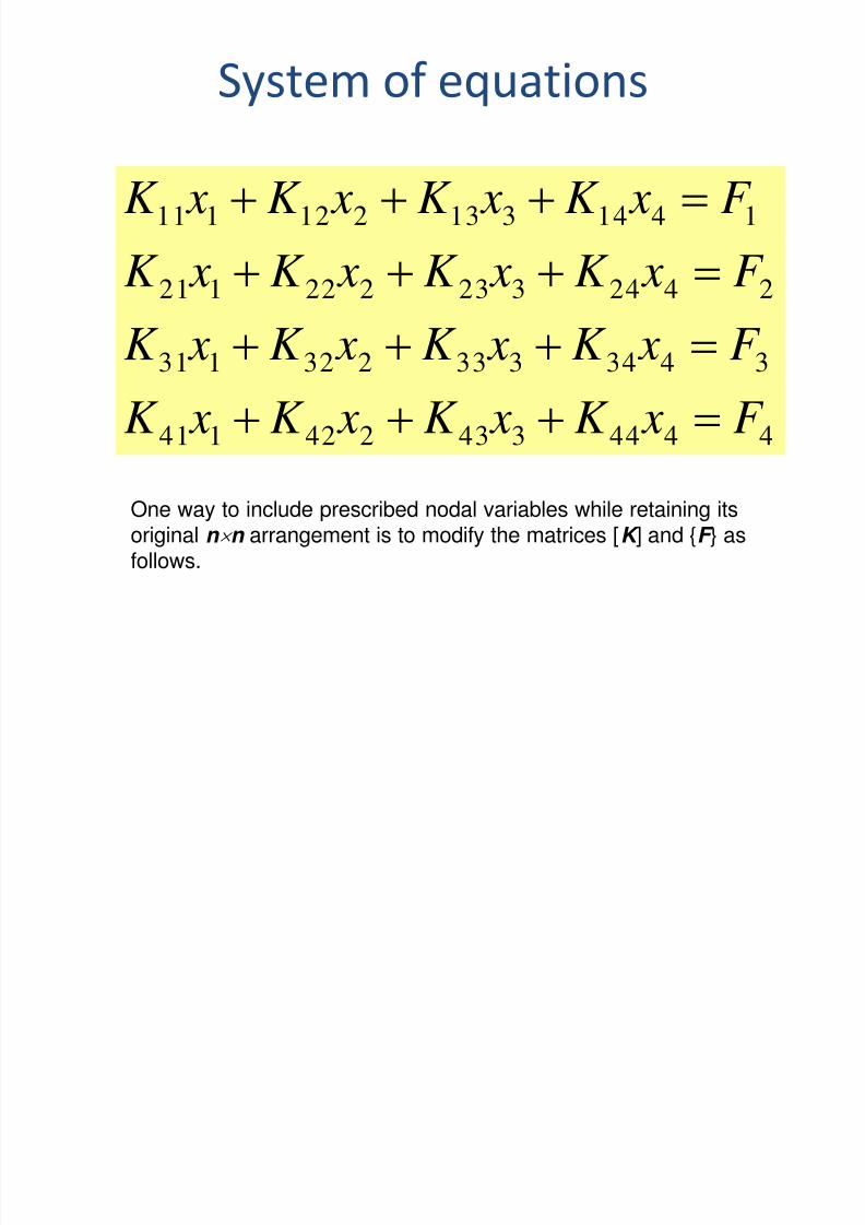
System of equations
4444343242141
3434333232131
2424323222121
1414313212111
F xK xK xK xK
F xK xK xK xK
F xK xK xK xK
F xK xK xK xK
One way to include prescribed nodal variables while retaining itsoriginal n n arrangement is to modify the matrices [K ] and {F } asfollows.
8/4/2019 ZINT1001 - Engineering Computational Tools - Part C - Engineering Applications
http://slidepdf.com/reader/full/zint1001-engineering-computational-tools-part-c-engineering-applications 25/47
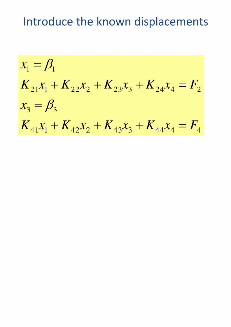
Introduce the known displacements
4444343242141
33
2424323222121
11
F xK xK xK xK
x
F xK xK xK xK
x
8/4/2019 ZINT1001 - Engineering Computational Tools - Part C - Engineering Applications
http://slidepdf.com/reader/full/zint1001-engineering-computational-tools-part-c-engineering-applications 26/47
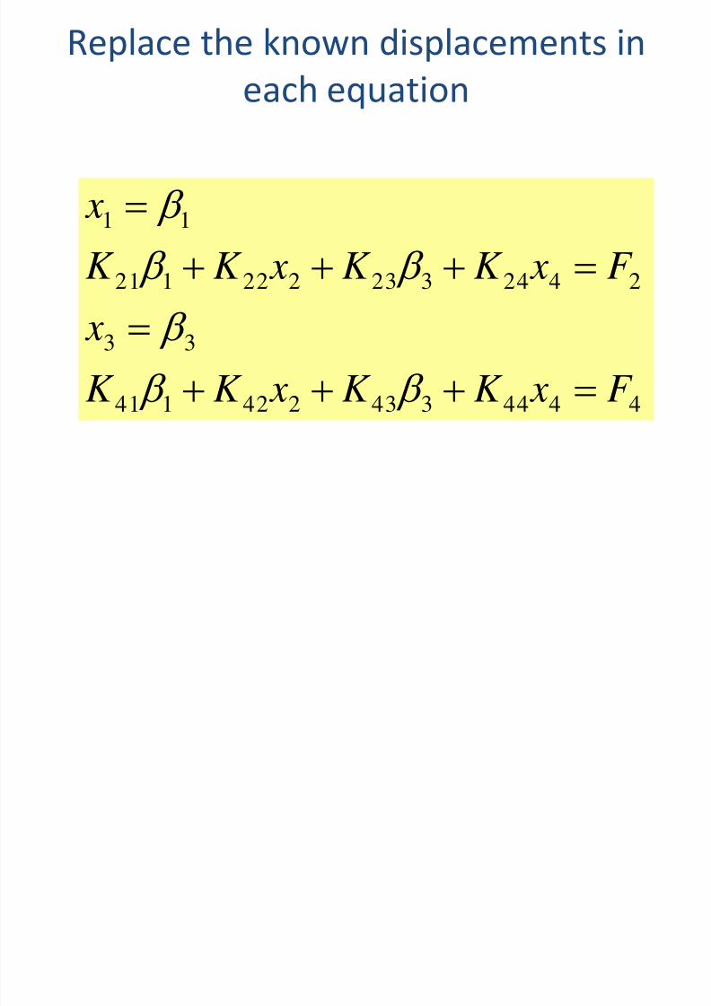
Replace the known displacements in
each equation
4444343242141
33
2424323222121
11
F xK K xK K
x
F xK K xK K
x
8/4/2019 ZINT1001 - Engineering Computational Tools - Part C - Engineering Applications
http://slidepdf.com/reader/full/zint1001-engineering-computational-tools-part-c-engineering-applications 27/47
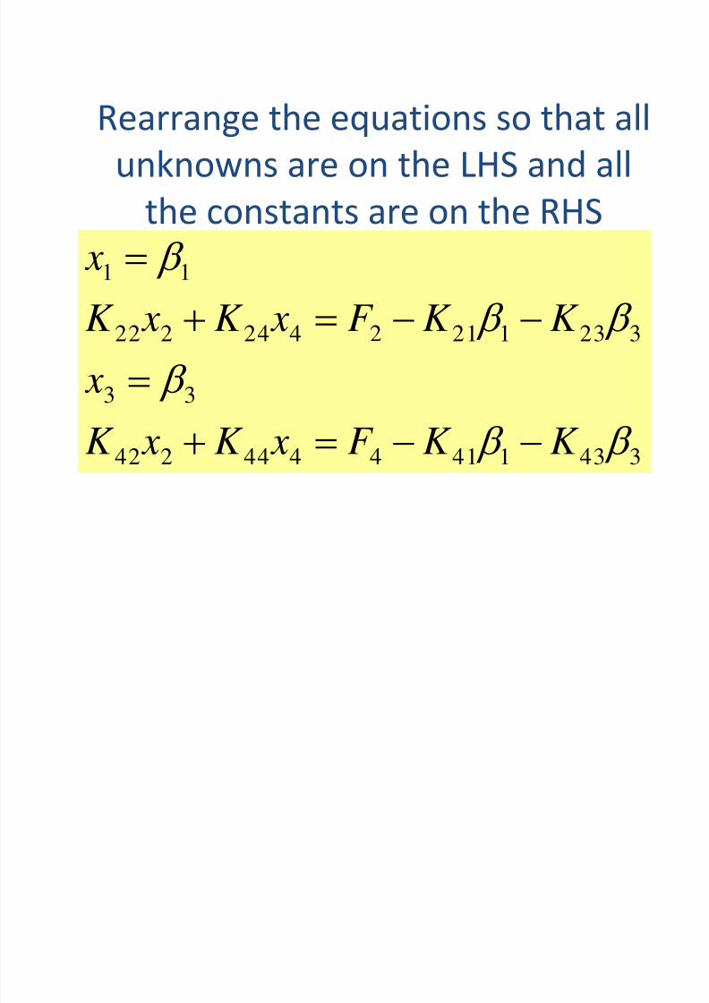
Rearrange the equations so that allunknowns are on the LHS and all
the constants are on the RHS
3431414444242
33
3231212424222
11
K K F xK xK
x
K K F xK xK
x
8/4/2019 ZINT1001 - Engineering Computational Tools - Part C - Engineering Applications
http://slidepdf.com/reader/full/zint1001-engineering-computational-tools-part-c-engineering-applications 28/47
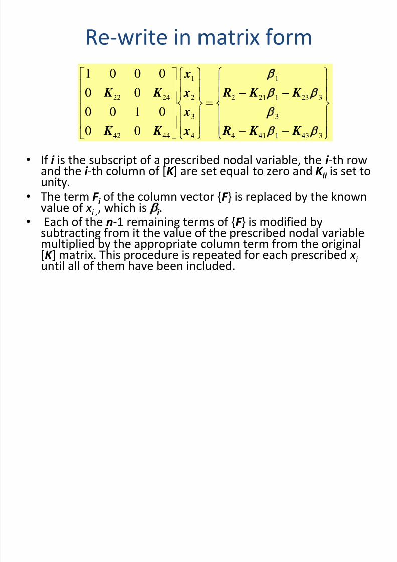
Re-write in matrix form
1 0 0 0
0 0
0 0 1 0
0 0
22 24
42 44
1
2
3
4
1
2 21 1 23 3
3
4 41 1 43 3
K K
K K
x
x
x
x
R K K
R K K
• If i is the subscript of a prescribed nodal variable, the i -th rowand the i -th column of [K ] are set equal to zero and K
ii is set to
unity.• The term F
i of the column vector {F } is replaced by the known
value of x i ,, which is i .• Each of the n-1 remaining terms of {F } is modified by
subtracting from it the value of the prescribed nodal variablemultiplied by the appropriate column term from the original[K ] matrix. This procedure is repeated for each prescribed x i until all of them have been included.
8/4/2019 ZINT1001 - Engineering Computational Tools - Part C - Engineering Applications
http://slidepdf.com/reader/full/zint1001-engineering-computational-tools-part-c-engineering-applications 29/47
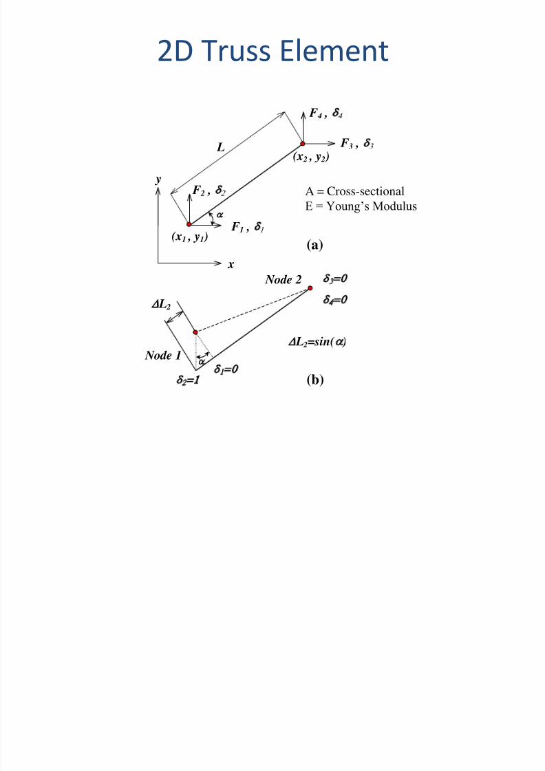
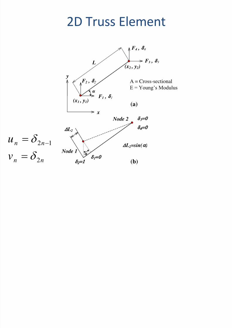
2D Truss Element
y
x
F 4 ,
L
A = Cross-sectionalE = Young’s Modulus
L 2
Node 1
Node 2
(a)
F 3 ,
(x 2 , y 2 )
(x1 , y1 ) F1 ,
F 2 ,
L 2=sin( )
(b)
8/4/2019 ZINT1001 - Engineering Computational Tools - Part C - Engineering Applications
http://slidepdf.com/reader/full/zint1001-engineering-computational-tools-part-c-engineering-applications 30/47
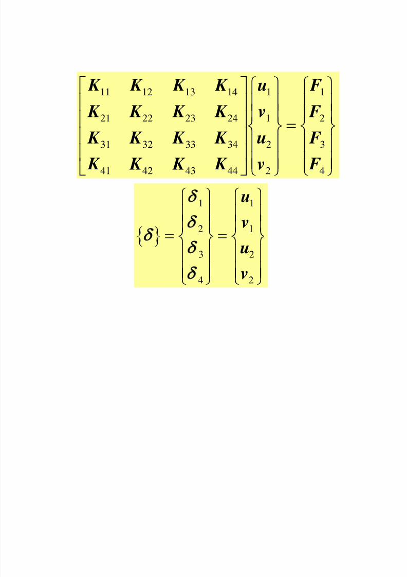
K K K K
K K K K
K K K K K K K K
u
v
uv
F
F
F F
11 12 13 14
21 22 23 24
31 32 33 34
41 42 43 44
1
1
2
2
1
2
3
4
1
2
3
4
1
1
2
2
u
v
u
v
8/4/2019 ZINT1001 - Engineering Computational Tools - Part C - Engineering Applications
http://slidepdf.com/reader/full/zint1001-engineering-computational-tools-part-c-engineering-applications 31/47
2D Truss Element
y
x
F 4 ,
L
A = Cross-sectionalE = Young’s Modulus
L 2
Node 1
Node 2
(a)
F 3 ,
(x 2 , y 2 )
(x1 , y1 ) F1 ,
F 2 ,
L 2=sin( )
(b)nn
nn
v
u
2
12
8/4/2019 ZINT1001 - Engineering Computational Tools - Part C - Engineering Applications
http://slidepdf.com/reader/full/zint1001-engineering-computational-tools-part-c-engineering-applications 32/47
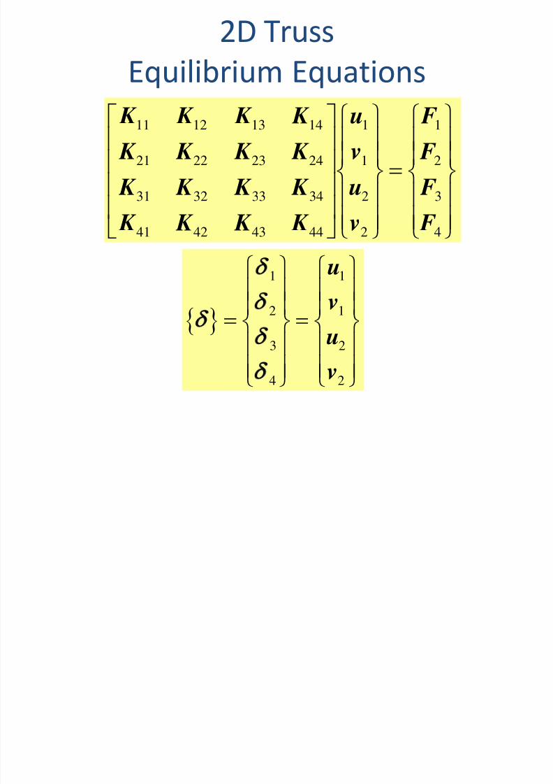
2D Truss
Equilibrium Equations
K K K K
K K K K
K K K K K K K K
u
v
uv
F
F
F F
11 12 13 14
21 22 23 24
31 32 33 34
41 42 43 44
1
1
2
2
1
2
3
4
1
2
3
4
1
1
2
2
u
v
u
v
8/4/2019 ZINT1001 - Engineering Computational Tools - Part C - Engineering Applications
http://slidepdf.com/reader/full/zint1001-engineering-computational-tools-part-c-engineering-applications 33/47

8/4/2019 ZINT1001 - Engineering Computational Tools - Part C - Engineering Applications
http://slidepdf.com/reader/full/zint1001-engineering-computational-tools-part-c-engineering-applications 34/47
y
x
F 4
F 3
F1
F 2 F
ode 1
ode 2
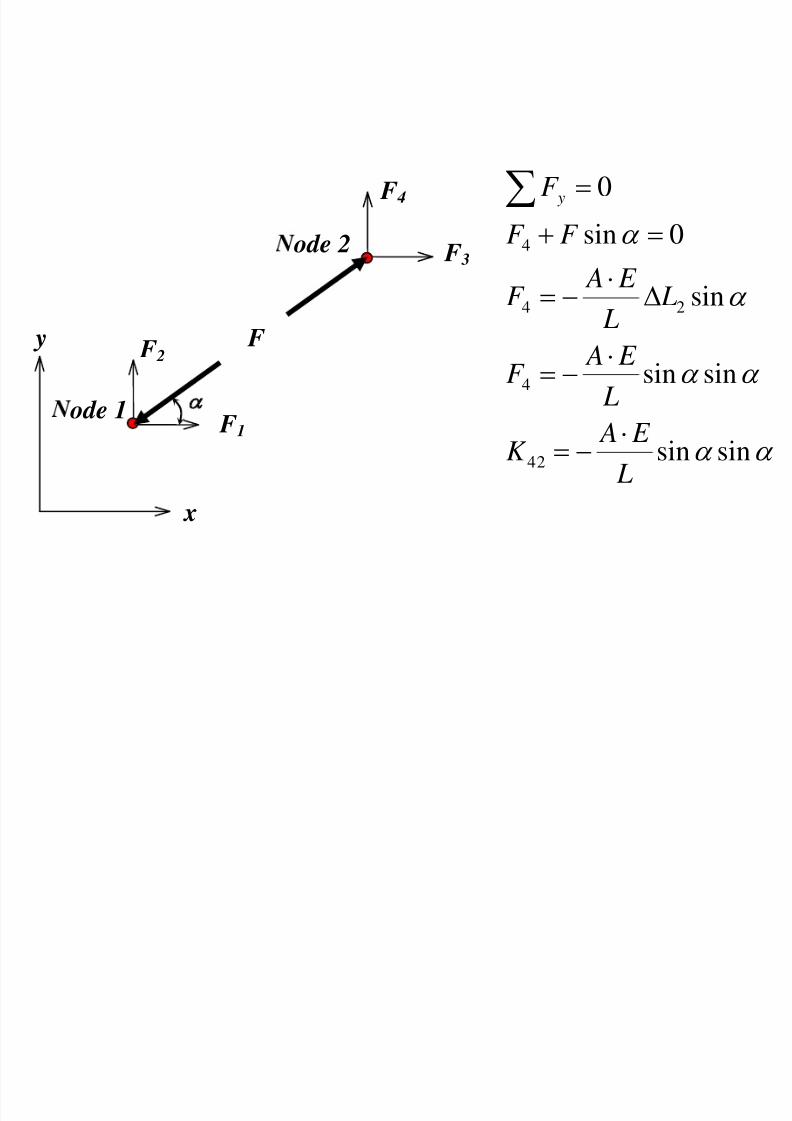
sinsin
sinsin
sin
0sin
0
22
2
22
2
L
E AK
L
E AF
L L
E AF
F F
F y

8/4/2019 ZINT1001 - Engineering Computational Tools - Part C - Engineering Applications
http://slidepdf.com/reader/full/zint1001-engineering-computational-tools-part-c-engineering-applications 35/47
y
x
F 4
F 3
F1
F 2 F
ode 1
ode 2
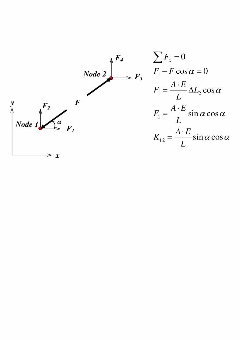
cossin
cossin
cos
0cos
0
32
3
23
3
L
E AK
L
E AF
L L
E AF
F F
F x
8/4/2019 ZINT1001 - Engineering Computational Tools - Part C - Engineering Applications
http://slidepdf.com/reader/full/zint1001-engineering-computational-tools-part-c-engineering-applications 36/47
8/4/2019 ZINT1001 - Engineering Computational Tools - Part C - Engineering Applications
http://slidepdf.com/reader/full/zint1001-engineering-computational-tools-part-c-engineering-applications 37/47
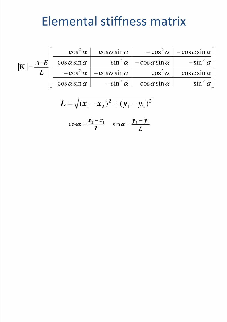
Elemental stiffness matrix
22
22
22
22
sinsincossinsincos
sincoscossincoscos
sinsincossinsincos
sincoscossincoscos
L
E AK
L x x y y ( ) ( )1 2
2
1 2
2
cos x x L
2 1 sin y y L
2 1
8/4/2019 ZINT1001 - Engineering Computational Tools - Part C - Engineering Applications
http://slidepdf.com/reader/full/zint1001-engineering-computational-tools-part-c-engineering-applications 38/47
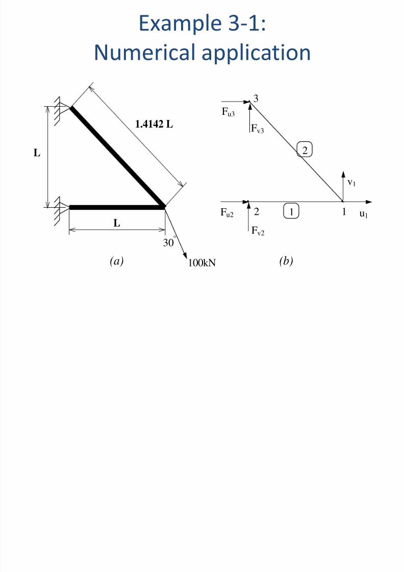
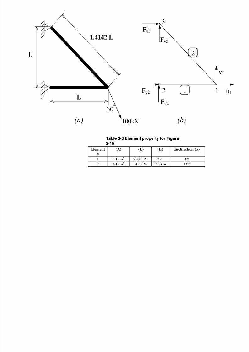
Example 3-1:
Numerical application
L
L
1.4142 L
30
100kN
Fv2
Fu2
Fv3
Fu3
u1
v1
2
2 1
3
1
(a) (b)
8/4/2019 ZINT1001 - Engineering Computational Tools - Part C - Engineering Applications
http://slidepdf.com/reader/full/zint1001-engineering-computational-tools-part-c-engineering-applications 39/47

8/4/2019 ZINT1001 - Engineering Computational Tools - Part C - Engineering Applications
http://slidepdf.com/reader/full/zint1001-engineering-computational-tools-part-c-engineering-applications 40/47
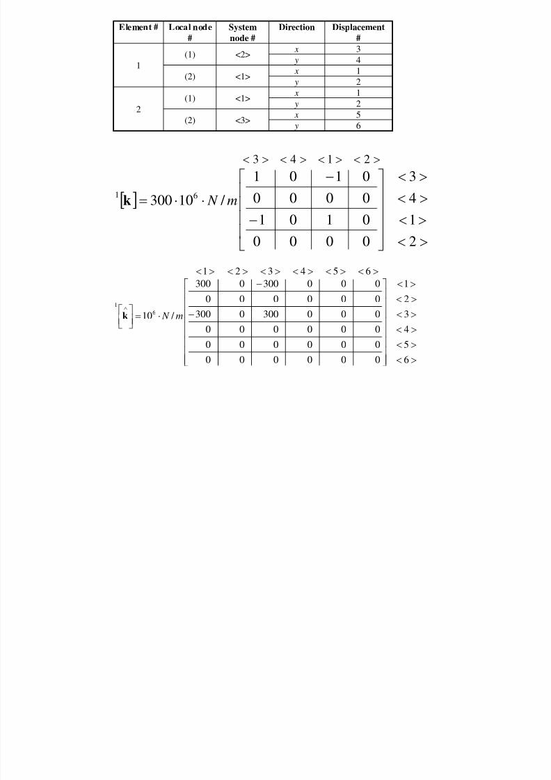
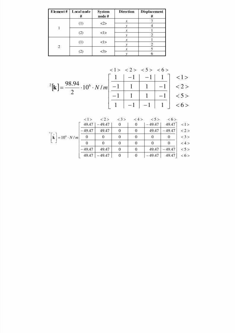
Element # Local node
#
System
node #
Direction Displacement
#
1
(1) <2>x 3
y 4
(2) <1>x 1
y 2
2
(1) <1>x 1
y 2
(2) <3>x 5
6
Table 3-4 Correspondence between local and global numbering
schemes
L
L
1.4142 L
30
100kN
Fv2
Fu2
Fv3
Fu3
u1
v1
2
2 1
3
1
(a) (b)
nn
nn
v
u
2
12
8/4/2019 ZINT1001 - Engineering Computational Tools - Part C - Engineering Applications
http://slidepdf.com/reader/full/zint1001-engineering-computational-tools-part-c-engineering-applications 41/47
2
1
4
3
0000
0101
0000
01 01
/ 10300
2143
61 m N k
Element # Local node
#
System
node #
Direction Displacement
#
1
(1) <2>x 3
y 4
(2) <1>x 1
y 2
2(1) <1>
x 1
y 2
(2) <3>x 5
y 6
6
5
4
3
2
1
000000
000000
000000
0003000300
000000
0003000300
654321
/ 106
1
m N k
8/4/2019 ZINT1001 - Engineering Computational Tools - Part C - Engineering Applications
http://slidepdf.com/reader/full/zint1001-engineering-computational-tools-part-c-engineering-applications 42/47
Element # Local node
#
System
node #
Direction Displacement
#
1
(1) <2>x 3
y 4
(2) <1>x 1
y 2
2(1) <1>
x 1
y 2
(2) <3>x 5
y 6
6
5
2
1
1111
1111
1111
11 11
/ 10294.98
6521
62 m N k
6
5
4
3
21
47.4947.490047.4947.49
47.4947.490047.4947.49
000000
000000
47.4947.490047.4947.4947.4947.490047.4947.49
65432 1
/ 106
2
m N k
8/4/2019 ZINT1001 - Engineering Computational Tools - Part C - Engineering Applications
http://slidepdf.com/reader/full/zint1001-engineering-computational-tools-part-c-engineering-applications 43/47
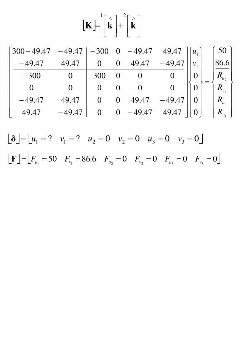
50
8/4/2019 ZINT1001 - Engineering Computational Tools - Part C - Engineering Applications
http://slidepdf.com/reader/full/zint1001-engineering-computational-tools-part-c-engineering-applications 44/47
3
3
2
2
6.86
50
0
0
00
1
1
v
u
v
u
R
R
R R
v
u
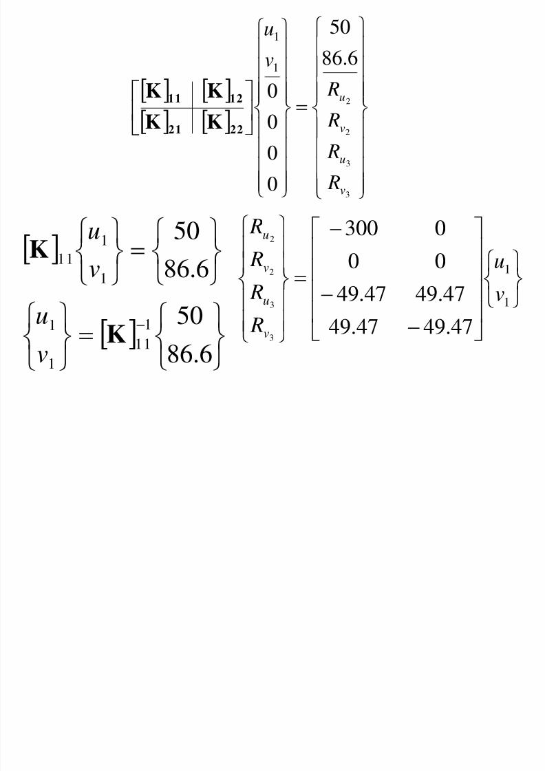
2221
1211
KKKK
6.86
50
1
1
11v
uK
6.86
501
11
1
1K
v
u
1
1
47.4947.49
47.4947.49
00
0300
3
3
2
2
v
u
R
R
R
R
v
u
v
u
8/4/2019 ZINT1001 - Engineering Computational Tools - Part C - Engineering Applications
http://slidepdf.com/reader/full/zint1001-engineering-computational-tools-part-c-engineering-applications 45/47
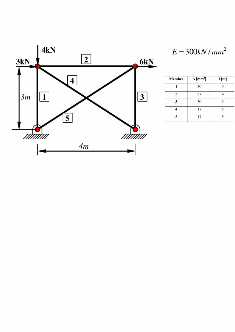
1
2
3
4
5
3m
4m
4kN
3kN 6kN
2 / 300 mmkN E
Member A [mm2] L[m]
1 30 3
2 27 4
3 30 3
4 17 5
5 17 5
21 23 4

8/4/2019 ZINT1001 - Engineering Computational Tools - Part C - Engineering Applications
http://slidepdf.com/reader/full/zint1001-engineering-computational-tools-part-c-engineering-applications 46/47
Global Node # x-coordinate [m] y-coordinate [m] Displacement #
1 0 01
2
2 4 03
4
3 0 35
6
4 4 3
7
8
1
2
3
4
5
1 2
1
2
1
2
1
2
1
2
1 2
3 4
x
yGlobal Coordinate
System (GCS)
element
element node
ystem node
nn
nn
v
u
2
12
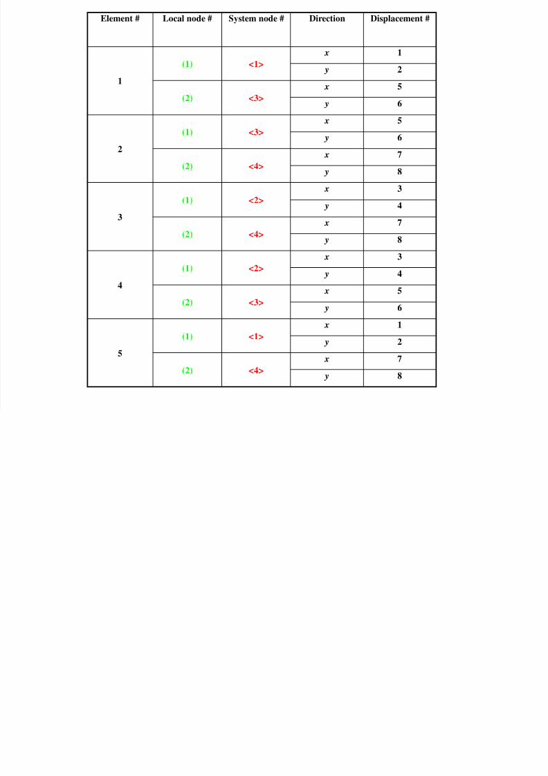
Element # Local node # System node # Direction Displacement #
8/4/2019 ZINT1001 - Engineering Computational Tools - Part C - Engineering Applications
http://slidepdf.com/reader/full/zint1001-engineering-computational-tools-part-c-engineering-applications 47/47
y p
1
(1) <1>
x 1
y 2
(2) <3>
x 5
y 6
2
(1) <3>
x 5
y 6
(2) <4>
x 7
y 8
3
(1) <2>
x 3
y 4
(2) <4>
x 7
y 8
4
(1) <2>
x 3
y 4
(2) <3> x 5
y 6
5
(1) <1>
x 1
y 2
(2) <4>
x 7
y 8