zhaoying han dissertation submitted to the faculty of...
TRANSCRIPT

EFFECT OF NON-RIGID REGISTRATION ALGORITHMS ON THE ANALYSIS OF
BRAIN MR IMAGES WITH DEFORMATION BASED MORPHOMETRY
By
Zhaoying Han
Dissertation
Submitted to the Faculty of the
Graduate School of Vanderbilt University
in partial fulfillment of the requirements
for the degree of
DOCTOR OF PHILOSOPHY
in
Electrical Engineering
Dec, 2011
Nashville, Tennessee
Approved:
Professor Benoit M. Dawant
Professor John C. Gore
Professor J. Michael Fitzpatrick
Professor Adam W. Anderson
Professor Zhaohua Ding
Professor Bennett A. Landman

ii
To my beloved parents
and
To my dear sister Ruthie
iii
ACKNOWLEDGEMENTS
Words cannot express the depth of my gratitude to all those who have helped to
make this dissertation possible. Above all, I would like to express my deepest gratitude to
my advisor Dr. Benoit Dawant for his guidance, wisdom, encouragement, help and great
patience. No doubt, this dissertation would never have moved passed the beginning
stages without him. I’m very thankful for Dr. Dawant for offering me this incredible,
humbling opportunity to study at Vanderbilt University in 2005; it was he who opened up
the door for me to pursue my dream of being a Ph.D. in the U.S. After I joined his lab, Dr.
Dawant taught me important image analysis techniques, broadened my horizons in the
applications of those techniques, trained me how to think logically and critically in
research, and inspired me to work diligently and persevere. I must note my enjoyment of
doing research with Dr. Dawant; he is always willing to discuss research problems and
offer great insights. He also spent numerous evenings and weekends to help me on my
projects and writing. Dr. Dawant is a great role model for me in terms of both research
and character; I also really appreciate his wise advice regarding career decisions. I am
beyond proud to have him as my advisor. Finally, I thank Dr. Dawant for the delicious
Belgian Chocolates over the years and the coffee maker he offered me on my second day
in the lab.
It is a great honor for me to have the chance to work with Dr. John Gore. I really
appreciate the privilege of being part of the Vanderbilt University Institute of Imaging
Sciences (VUIIS) since 2006. Dr. Gore has not only taught me Medical Image theory in
class, but also provided me many opportunities to learn cutting edge research in medical

iv
imaging. I really appreciate the various training opportunities in VUIIS, such as the
annual retreat, the weekly seminar, conferences, and collaborations across disciplines. I
especially thank Dr. Gore for offering me financial support over the years and his full
support on the projects in my dissertation. Dr. Gore is an inspiring and humorous leader,
and I cherish every discussion with him regarding my work and more.
I would like to thank Dr. Fitzpatrick for teaching me image registration in my first
year; the course served as a solid foundation in my research. It is an honor to work with
him and learn the meaning of rigorous research attitude. I also want to acknowledge Dr.
Anderson for his support of my research. I have hugely benefited from discussions with
him about the project on children with mathematical difficulties. Sincere thanks are also
due Dr. Zhaohua Ding for his consistent help and wise advice during my study. He has
taught me how to use Statistical Parametric Mapping (SPM), an important tool in my
research. I also appreciate his collaboration on the Williams Syndrome project. Next, I
would like to thank Dr. Landman for providing me an opportunity to work with him for
one semester. He helped me with the software pipeline development and provided
computation resources needed in the pipeline. I also really appreciate his help in
understanding key concepts in the statistical analysis and his valuable discussions on the
simulation work. Thanks also for the wonderful time with his lab members at work and
celebrating birthdays.
I really appreciate everyone at the Medical Image Processing Lab for their
friendship, valuable discussion, and assistance. Special thanks go to: Rui Li, Xia Li, Siyi
Ding, Antong Chen, Sri Pallavaram, Ankur Kumar, Anusha Rao, Jeremy Lecoeur, and
Yuan Liu. I want to thank my collaborators at VUIIS: Dr. Tricia Thornton-Wells, Dr.

v
Nikki Davis, Christopher Cannistraci, and Aize Cao. Also, I would like to thank Andrew
Asman for his help on the pipeline software. Thanks are due to Xue Yang and Muqun Li
for their helpful discussions and friendship. I’d like to thank the ACCRE cluster at
Vanderbilt University to offer great computation resources to make my research possible.
Thanks especially Zhiao Shi for his consistent and patient help on ACCRE questions. I’m
also grateful for Sandy Winter and Linda Koger for being incredibly helpful with
administrative work.
These years spent pursuing my Ph.D. has been the best part of my life so far. I
have not only gained technical knowledge, but also have been able to know the real
meaning of life and my purpose here on earth. I want to thank the person who has had the
most lasting impact on me over these last few years -- my best friend and sister Ruthie.
She shared the Good News of Jesus with me and I became her sister on October 31, 2006
outside of Starbucks on 21st Avenue. Over the last five years, she is always by my side,
encouraging me when I am weak, and helping me become the person I was created to be.
I am eternally grateful for and impacted by her friendship and unconditional love. I also
want to thank the friends who encourage me consistently and help me in both the small
and large details of my life: Dave Mennen, Andrew Siao, Haoxiang Luo, Qiufeng Lin,
Luping Lin, Yaping Huang, Weiyi Xia, Lihong Wang, Angel Yang, Lu Sun, and more.
Thanks to my brothers and sisters for their faithful prayers for me during the thesis
writing process. Each of them means so much to me, and I love them. Lastly, I’d like to
express my deepest gratitude to my parents. Their infinite love helped me through every
step of my life; though oceans apart, they are always only a phone call away to be there
for me and support me.

vi
Thanks to my Heavenly Father and Lord Jesus Christ for calling me His daughter,
leading me out of darkness into his wonderful light, protecting me, and never leaving my
side. Without Christ as my personal Lord and Savior, my life would be void of the richest
gifts and relationships -- and I would never have arrived at this monumental day where I
stand before you to become a Ph.D. As a child, I dreamed the impossible: I wanted to
become a doctor in America. As a simple girl from a countryside town in Northern China
-- it was ridiculous for me to entertain such ambitions. Less than 1% of my high school
attended college and at times my family barely had enough food to eat. But day after day,
I pedaled my bike back and forth to school through the biting sandstorms -- determined to
make my dream a reality. Today, my dream has become reality.
Your word is a lamp for my feet, a light on my path. – Psalm 119:105
Natalie Zhaoying Han, 2011, Nashville.
vii
TABLE OF CONTENTS
Content Page
ACKNOWLEDGEMENTS ............................................................................................... iii
LIST OF TABLES ...............................................................................................................x
LIST OF FIGURES ........................................................................................................... xi
CHAPTER
CHAPTER 1: INTRODUCTION ........................................................................................1
1.1 DEFORMATION BASED MORPHOMETRY (DBM) ..........................................3
1.1.1 A Brief Background on DBM Analysis .....................................................3
1.1.2 The Overview of DBM Analysis ...............................................................5
1.2 NON-RIGID REGISTRATION ALGORITHMS .....................................................7
1.2.1 A Brief Review of Comparisons of Registration Algorithms ....................7
1.2.2 Adaptive Bases Algorithm (ABA) .............................................................8
1.2.3 Image Registration Toolkit (IRTK) .........................................................10
1.2.4 FSL Nonlinear Image Registration Tool (FSL) .......................................12
1.2.5 Automatic Registration Toolbox (ART) ..................................................14
1.2.6 SPM Normalization (SPM) ......................................................................15
1.3 GROUP ATLAS CREATION ................................................................................17
1.3.1 Data Preprocessing...................................................................................17
1.3.2 Overview of Group Specific Atlas Creation ............................................19
1.3.3 Atlases Based on Affine Registration ......................................................21
1.3.4 Atlases Based on Non-rigid Registrations ...............................................22
1.4 OVERVIEW OF THIS DISSERTATION..............................................................25

viii
CHAPTER 2: EFFECT OF NON-RIGID REGISTRATION ALGORITHMS ON
DEFORMATION BASED MORPHOMETRY: A COMPARATIVE STUDY
WITH CONTROL AND WILLIAMS SYNDROME SUBJECTS ...................................27
2.1 INTRODUCTION ..................................................................................................27
2.2 MATERIALS AND METHODS ............................................................................29
2.2.1 Data and Preprocessing ............................................................................29
2.2.2 Creation of Group Atlases .......................................................................30
2.2.3 Non-rigid Registration Algorithms ..........................................................32
2.2.4 Features Used in our DBM Analysis .......................................................34
2.2.5 Statistical Analysis ...................................................................................35
2.2.6 Comparisons of DBM Results .................................................................36
2.3 RESULTS ................................................................................................................37
2.3.1 Effects of Registrations on Group Atlas ..................................................37
2.3.2 Raw T maps .............................................................................................40
2.3.3 DBM Results Obtained with the JAC and DFM Features .......................42
2.3.4 Relating DBM Findings to Observable Anatomical Differences ............46
2.4 DISCUSSION ..........................................................................................................52
CHAPTER 3: RELATION BETWEEN CORTICAL ARCHITECTURE AND
MATHEMATICAL ABILITY IN CHILDREN: A DBM STUDY ..................................58
3.1 INTRODUCTION ...................................................................................................58
3.2 MATERIALS AND METHODS .............................................................................61
3.2.1 Data Description ......................................................................................61
3.2.2 Creation of Group Atlases .......................................................................62
3.2.3 Group Differences Identified with DBM .................................................63
3.2.4 Correlation of DBM Findings with Math Scores .....................................65
3.3 RESULTS ................................................................................................................67
3.3.1 Group Differences Detected with DBM Analysis of the JAC
Feature......................................................................................................67
3.3.2 Group Differences Detected with DBM Analysis of the DFM
Feature......................................................................................................71

ix
3.3.3 Group Differences Detected with DBM Analysis of the Voxel-
wise Correlation Coefficient between the DFM Feature and the
WRAT-M Score. .....................................................................................76
3.4 DISCUSSION .......................................................................................................81
CHAPTER 4: AN ANALYSIS OF THE EFFECT OF NONRIGID
REGISTRATION ALGORITHMS ON DBM ANALYSIS USING SIMULATED
DATASETS .......................................................................................................................85
4.1 INTRODUCTION ..................................................................................................85
4.2 METHOD ................................................................................................................88
4.2.1. Simulation with the SSD Model .............................................................89
4.2.2. Simulation with the Growth Models .......................................................91
4.2.3. Deformation-based Morphometry (DBM) Analysis ...............................94
4.2.4 Quantitative Comparisons ........................................................................96
4.3 RESULTS ................................................................................................................98
4.3.1. Simulated Images with the SSD Model ..................................................98
4.3.2. Simulated Images with the Growth Models..........................................100
4.3.3. Qualitative Comparisons of Registration Algorithms...........................102
4.3.4. Quantitative Comparisons of Registration Algorithms.........................105
4.4 DISCUSSION ........................................................................................................107
CHAPTER 5: SUMMARY AND FUTURE WORK ......................................................109
References ........................................................................................................................114
x
LIST OF TABLES
Table Page
Table. I. 1. Comparison of non-rigid registration methods in terms of their outputs
for atlas creation .................................................................................................................23
Table. II. 1. Summary of DBM results based on JAC over three ROIs. *means
corrected p >0.05. † means FSL has a contiguous region, and we treated it as two
clusters divided by the inter-hemisphere fissure. ...............................................................46
Table. II. 2. Summary of DBM results based on DFM over two ROIs. *means
corrected p> 0.05. ..............................................................................................................46
Table. III. 1. Summaries of DBM results based on DFM over three ROIs based on
different registration algorithms. * means the region found only by IRTK with
corrected p of 0.05. Green/blue colors mean this region is significant with
corrected p of 0.5/0.05 by that algorithm. ..........................................................................75
Table. IV. 1. Summaries of DBM results of JAC based on different registration
algorithms comparing to the grond truth, in terms of TP, FP and CDR, for eight
GM1 and GM2 derived groups. .......................................................................................105

xi
LIST OF FIGURES
Figure Page
Fig. I. 1.The overview of the deformation-based morphometry (DBM) method ............... 6
Fig. I. 2. Before (upper row) and after (lower row) N3 intensity correction for one
MR image...........................................................................................................................17
Fig. I. 3. A-a coronal view of a subject; B – The MNI152 template; C- After
direct rigid registration to MNI152 template; D – Affine registration first, and
then extract the rigid registration parameter to deform the image. ....................................19
Fig. I. 4. Schematic representation of the atlas creation process used in our study .......... 20
Fig. I. 5. Effect of initial reference selection on population averages for the whole
population. Top panels in (a) and (b): the axial and coronal views of two different
initial references; bottom panels in (a) and (b): the axial and coronal views of the
average brain model atlases obtained from the corresponding initial reference
volumes. .............................................................................................................................21
Fig. I. 6. The affine atlases for two different groups. The first column shows the
reference volumes in each group, the second column shows the averaged image
after the first iteration The third column shows the atlases shown in column two
deformed with the averaged inverse deformation fields. The fourth and fifth
columns show the affine atlases after the second and third iterations. ..............................22
Fig. II. 1. Region selection for DBM results comparison. ................................................ 36

xii
Fig. II. 2. The creation of group atlases for NC (top panel) and WS (middle panel)
group using registration algorithms (from left to right): ABA, IRTK, FSL, ART,
SPM. The image differences are shown at the bottom. .....................................................38
Fig. II. 3. Central sulcus tracing on the group atlases for NC (top panel, red lines)
and WS (bottom panel, green lines) groups using registration algorithms (from
left to right): ABA, IRTK, FSL, ART, and SPM. ..............................................................39
Fig. II. 4. CC shape differences between NC and WS. ..................................................... 40
Fig. II. 5. Effect of registration on Corpus Callosum (CC) shape differences for
NC and WS atlases.............................................................................................................40
Fig. II. 6. T maps on JAC (top row) and DFM (bottom row) using different
registration algorithms. ......................................................................................................41
Fig. II. 7. Smoothness estimation (FWHM in X, Y and Z directions) for JAC and
DFM T maps for different registration algorithms (from left to right): ABA, IRTK,
FSL, ART, and SPM. .........................................................................................................41
Fig. II. 8. DBM results based on JAC differences between NC and WS groups. ............ 45
Fig. II. 9. DBM results based on DFM differences between NC and WS groups. ........... 45
Fig. II. 10. Scheme used for affine registration of group atlases to the DBM atlas
(highlight of observable differences). ................................................................................47
Fig. II. 11. Top panel: A) deformed NC atlas, B) DBM atlas, C) deformed WS
atlas, and D) Image differences between A and C (Colormap range: [-160,160]).
Bottom panel: The DBM results for JAC based on a) ABA, b) IRTK, c) FSL, and

xiii
d) ART. The pink and cyan lines were drawn on the deformed NC and WS atlas
respectively. .......................................................................................................................48
Fig. II. 12. Top panel: A) deformed NC atlas, B) DBM atlas, C) deformed WS
atlas, and D) Image differences between A and C (Colormap range: [-160,160]).
Bottom panel: The DBM results for JAC based on a) ABA, b) IRTK, c) FSL, and
d) ART. The pink and cyan lines were drawn on the deformed NC and WS atlas
respectively ........................................................................................................................50
Fig. II. 13. Top panel: A:) deformed NC atlas, B) DBM atlas, C) deformed WS
atlas, D) Image differences between A and B (Colormap range: [-160,160]).
Middle panel: The DBM results obtained with the DFM feature with different
registration algorithms superimposed on the DBM atlas. Bottom panel: The DBM
results obtained with the JAC feature with different registration algorithms
superimposed on the DBM atlas. The cyan and pink lines delineate the boundary
of the right anterior insular cortex drawn on the deformed WS and NC atlas
respectively. .......................................................................................................................51
Fig. III. 1. Smoothness estimation (FWHM in X, Y and Z directions) for JAC (left)
and DFM (right) T maps for different registration algorithms (from left to right):
ABA, IRTK, FSL, ART, and SPM. ...................................................................................67
Fig. III. 2. The color-coded T maps of the voxel-wise T-test analysis on the JAC
features between the NC and the MD group based on five non-rigid registration
algorithms. Each row displays selected slices in the T maps obtained based on one
algorithm, from the top to the bottom: ABA, IRTK, FSL, ART and SPM. ......................69
Fig. III. 3. The regions with different ranges of p values for DBM results for JAC
based on each registration algorithm superimposed on one volume deformed to
the DBM atlas. Warm colors show NC has larger JAC than MD, and cold colors

xiv
mean the opposite. None of these clusters survived the FWE multiple comparison
correction. ..........................................................................................................................70
Fig. III. 4. The color-coded T maps of the voxel-wise T-test analysis on the DFM
features between the NC and the MD group based on five non-rigid registration
algorithms. Each row displays the selected slices in the T maps obtained with one
algorithm, from the top to the bottom: ABA, IRTK, FSL, ART and SPM. ......................73
Fig. III. 5. The regions with different ranges of p values for DBM results for DFM
based on each registration algorithm superimposed on one volume deformed to
the DBM atlas. Warm colors show that NC has larger DFM than MD, and cold
colors mean the opposite. ...................................................................................................74
Fig. III. 6. The common ROIs in the DBM results of DFM difference between NC
and MD groups. All clusters are statistically significant after FWE correction and
superimposed on one volume deformed to the DBM atlas. Three ROIs were
identified and circled with different colors. The line type means different
statistical significance levels. .............................................................................................75
Fig. III. 7. The color-coded T maps of the voxel-wise ANCOVA analysis between
the DFM feature and WRAT-M scores for all the 79 children based on five non-
rigid registration algorithms. Each row displays three selected views of the T
maps obtained based on one algorithm, from the top to the bottom: ABA, IRTK,
FSL, ART and SPM. ..........................................................................................................77
Fig. III. 8. The regions with different ranges of p values for DBM results of DFM
correlated with WRAT-M scores based on each registration algorithm
superimposed on one volume deformed to the DBM atlas. Warm colors show that
NC has larger DFM than MD, and cold colors mean the opposite. ...................................78

xv
Fig. III. 9. Scattered plots for correlation analysis between the mean DFM over
each ROI and the WRAT-M scores for all the 79 children, using five different
registration algorithms. Red frames mean the correlation coefficients are
statistically significant (p<0.05), blue frames mean the opposite. .....................................79
Fig. IV. 1. The overview of the proposed framework. ................................................... 898
Fig. IV. 2. The various steps used to train the SSD models and to produce test
images. ...............................................................................................................................89
Fig. IV. 3. Coordinates conversion. .................................................................................. 91
Fig. IV. 4. The illustration of GM1 and GM2. ................................................................. 92
Fig. IV. 5. The displacement radius and growth radius for local growths in GM1
and GM2. ...........................................................................................................................93
Fig. IV. 6. The ground truth for each set of the growth model. ........................................ 94
Fig. IV. 7. The flowchart for DBM analysis on simulated datasets.................................. 95
Fig. IV. 8. FN, TP, FP. ...................................................................................................... 96
Fig. IV. 9. Examples of simulated images with the SSD model in G1 (top) and G2
(bottom) groups. .................................................................................................................98
Fig. IV. 10. Statistical analysis of JAC between the G1 and G2 groups. ......................... 99
Fig. IV. 11. Smoothness estimation (FWHM in X, Y, and Z directions) for JAC T
maps. ..................................................................................................................................99

xvi
Fig. IV. 12. An example of simulated images in the G2 group and four GM1
based groups. The zoomed views are shown in the middle panel, and bottom
panel shows the intensity differences. .............................................................................101
Fig. IV. 13. An example of simulated images in the G2 group and four GM2
based groups. The zoomed views are shown in the middle panel, and bottom
panel shows the intensity differences. .............................................................................101
Fig. IV. 14. Qualitative comparison of registration algorithms on DBM results of
JAC with the ground truth for 8 different sets of growth models (thresholded at
uncorrected p of 0.001). White circles mean that the cluster is not statistically
significant after FWE corrected p of 0.05. .......................................................................104
Fig. IV. 15. Cluster Detection Rate (CDR) for DBM using JAC before and after
FWE corrections (corrected p of 0.05) for GM1 and GM2 derived groups. ...................106
Fig. IV. 16. Cluster Detection Rate (CDR) for DBM using JAC when using FWE
corrected p of 0.1 and 0.5 for GM1 and GM2 derived groups ........................................107

1
CHAPTER 1
INTRODUCTION
With the tremendous pace of development in medical imaging technologies, the
ability to investigate brain structure and function has been revolutionized. High resolution
Magnetic Resonance Imaging (MRI) has emerged as the premier modality to provide
noninvasive means of visualizing the brain’s internal structures in detail. Brain
morphometric studies have been utilized to elucidate various anatomical feature
differences among populations, as well as to characterize correlations between neural
substrates and growth, degenerative processes, or gene expressions. Usually
morphometry analyses have been applied on regions of interests (ROIs) which can be
clearly defined, such as the hippocampus [1, 2] or the corpus callosum [3-5] that are
known to be associated with specific diseases. But for certain diseases or disabilities,
such a priori anatomical knowledge does not exist. In this situation, global approaches
are sought after to find anatomical differences throughout the entire brain.
This dissertation focuses on a global morphometric approach, called deformation-
based morphometry (DBM) [6, 7] which quantifies and characterizes morphometric
differences between brains on a voxel-by-voxel basis without any pre-defined ROIs.
DBM analysis, sometimes referred to as tensor-based morphometry (TBM), has been
carried out on a variety of populations, including patients with schizophrenia [8-12],
Alzheimer’s disease[13-15], and developmental or genetic disorders[16-25]. The DBM
approach requires images from different groups to be registered together to a brain atlas

2
(i.e. template) and statistically identifies morphological differences between groups based
on the deformation fields generated by a non-rigid registration algorithm. A number of
registration algorithms have been proposed over the years for this purpose [26-31].
Although several studies have compared non-rigid registration algorithms for segmentation
tasks [32-37], few studies have compared the effect of the registration algorithms on
population differences that may be uncovered through deformation-based morphometry
(DBM). The overarching goal of this dissertation is to assess qualitatively and quantitatively
the extent to which DBM results are a function of the registration algorithm used to compute
the deformation fields. Two very different real data sets and a series of simulated data sets
are used to compare these registration algorithms.
Brain atlases play an important role in DBM analysis, as they serve as the standard
coordinate system to which all brain images are aligned for subsequent comparison and
integration of DBM measurements. To avoid the bias introduced by a single volume,
group specific atlases are usually created to be representative of the predefined
populations using various techniques involving non-rigid registration [38-46]. We thus
investigate the effect of various non-rigid registration algorithms on the creation of group
specific atlases.
This chapter is organized as follows. Section 1.1 provides some background on
DBM and the various processing steps in details. Section 1.2 briefly reviews previous
work on non-rigid registration algorithms comparison. This is followed by a description
of each of the five non-rigid registration algorithms used in our study. Section 1.3 covers
the fundamental steps that have been used in this work for the creation of group specific
atlases. An overview of the remainder of the dissertation is presented in section 1.4.

3
1.1 DEFORMATION BASED MORPHOMETRY (DBM)
1.1.1 A Brief Background on DBM Analysis
Brain morphometric studies usually involve the images of multiple subjects being
aligned together by some form of spatial normalization. The two primary results
produced by the spatial normalization process are the deformed images and the
deformation fields that describe the transformations required to match each image
volume to a common template. Morphometric analyses can thus be broadly classified into
two categories: those that operate on the images and those that operate on the
deformation fields.
Examples of the first category of morphometric analysis which is not primarily
based on the analysis of the deformation fields includes voxel-based morphometry (VBM)
[47], morphometry based on the HAMMER [31] algorithm, or surface-based
morphometry (SBM). VBM, proposed by Ashburner et al. [47], involves spatially
normalizing all the images, extracting the gray matter from the normalized images,
smoothing and performing a voxel-wise statistical analysis to localize group differences.
Optimized VBM provides an option to modulate the segmented gray matter images with
the Jacobian determinants derived from the spatial normalization [48]. Morphometry
analysis based on the HAMMER registration algorithm, proposed by Shen and
Davatzikos [31, 49], involves the segmentation of white matter (WM), gray matter (GM),
the calculation of Regional Analysis of Volumes Examined in Normalized Space
(RAVENS) to account for anatomical volume changes produced by the non-rigid
registration process, and the statistical analysis on RAVENS maps. SBM relies on the

4
output of cortical surface segmentation and surface-based registration algorithms to find
statistical differences in the cortical thickness and surface areas [50-52]. Detailed
discussions of these techniques are beyond the scope of this study because they do not
exclusively rely on the deformation fields.
The second category of morphometric analysis techniques utilizes the information
from the deformation fields to characterize differences between groups; these techniques
include deformation-based morphometry (DBM) [7] and tensor-based morphometry
(TBM) [6, 47]. Many features of the deformation fields could be extracted and compared
to find group morphological differences. When the concept of DBM was first introduced,
DBM referred to two kinds of deformation field-derived features: 1) the parameters
describing the deformation fields, represented as a combination of nonlinear basis
functions [6, 7, 47]; 2) the full 3D deformation fields at each voxel [8]. Techniques
based on the full 3D deformation field became the mainstream approaches for DBM
because they provide more detailed and region specific information even though they
require substantial computational resources. The deformation field describes the
displacement at each and every voxel from one subject to the atlas. By taking the
gradients of the field at each point, a Jacobian matrix field can be computed. The field
obtained by taking the determinants of the Jacobian matrix at each voxel produces a map
that indicates local volume growth (Jacobian determinant greater than one) or reduction
(Jacobian determinant smaller than one). TBM (Tensor Based Morphometry) is usually
referred to as the morphometric techniques that use the Jacobian determinant to measure
voxel-wise volumetric changes between two groups (see for instance the work of
Thompson et al. [13, 19-22, 53] and others [24, 25, 54]). However, researchers like

5
Studholme et al. [16, 17], Evans et al. [12, 55-57], and others [57-61] also used the term
DBM when using the Jacobian matrix and Jacobian determinant as deformation field-
based features. In this dissertation, DBM is referred to as any approach that uses features
extracted from the deformation fields, including displacement vectors and the Jacobian
determinant. Group morphological differences are localized after statistical analysis on
these deformation field features. DBM does not require any segmentation tasks and prior
information on structures.
1.1.2 The Overview of DBM Analysis
Fig. I. 1 presents an overview of the general deformation-based morphometry
(DBM) technique used in this dissertation. Suppose a normal control (NC) group and a
subject group, which could be a number of subjects from the NC group at a different time
point or subjects from a population for which it is hypothesized that anatomical
differences exist. All the MR images in the two groups are first preprocessed and
spatially aligned using rigid/affine registration (see section 1.2.1). The two groups of
images are pooled together, a DBM atlas with average intensity and shape is constructed
(see section 1.2.2 for details), and all the images are registered to that atlas. Non-rigid
registrations from all images in each group to the DBM atlas yield a series of deformation
fields that describe the correspondence between the individual subject to the atlas. Two
DBM features are derived from these deformation fields: the deformation field magnitude
(DFM) and the Jacobian determinant (JAC). The deformation field magnitude at each
voxel is simply the length of the displacement vector that brings a voxel in one image
into correspondence in the other. This feature could be used as a biomarker to indicate

6
morphological shape and position variation. Morphological features of higher order, e.g.,
the Jacobian determinant, have been used to measure local volumetric expansion or
shrinkage.
Fig. I. 1. The overview of the deformation-based morphometry (DBM) method
Statistical analysis on the features extracted from the deformation fields is usually
performed using the Statistical Parametric Mapping (SPM) package (Wellcome
Department of Cognitive Neurology, London, UK http://www.fil.ion.ucl.ac.uk/spm/). In
practice, two sample t-tests are performed on a voxel basis, yielding a T map in SPM.
Multiple comparison issues are dealt with after the T map was thresholded at uncorrected
p of 0.001. Correction for multiple comparisons can be done by requiring a minimum
cluster size [8, 18], controlling the False Discovery Rate (FDR) [62], or the Family-wise
Error (FWE), as well as by nonparametric permutation tests [63]. Since the deformation
field is a slowly varying smooth field, the Random Field Theory (RFT) is often used to

7
calculate the FWE corrected p values (corrected p <0.05) to correct for multiple
comparisons; this is the method we have used in this work. Statistically significant
clusters after correction are usually color-coded and superimposed on the DBM atlas to
show the regions where two groups have morphological differences.
1.2 NON-RIGID REGISTRATION ALGORITHMS
Since DBM relies on the deformation fields generated by non-rigid registrations,
it is very important to assess and compare the effect of various registration techniques on
the performance of DBM analysis. We will first review previous work on non-rigid
registration comparison. This review will be followed by a brief introduction of the five
well-established non-rigid registration algorithms compared in this study: (1) The
Adaptive Bases Algorithm (ABA) [26], (2) The Image Registration Toolkit (IRTK) [27],
(3) The Automatic Registration Tools (ART) [28], (4) The FSL Nonlinear Image
Registration Tool (FNIRT) [64], and (5) The normalization algorithm available in SPM
[29].
1.2.1 A Brief Review of Comparisons of Registration Algorithms
Over the last five to ten years, a number of non-rigid registration algorithms have
been proposed but their comparison and evaluation is a difficult task. As opposed to
rigid-body problems for which a ground truth can be established and used to measure
registration accuracy [35], evaluation of algorithms designed for non-rigid registration
remains somewhat empirical. Several approaches have been proposed and studies

8
conducted to compare these algorithms using metrics such as tissue overlap measures [32,
36, 37, 65] or dispersion of homologous landmarks [28]. Klein et al. [33] conducted a
comprehensive study in which 14 algorithms are compared using tissue overlap measures
applied to human brain MRI images. Murphy et al. [34] provided a public platform for
comparison of 20 registration algorithms applied to intra-patient thoracic CT image pairs.
However, these studies are mostly based on the comparison of segmentation results
obtained with registration-based and manual segmentations in specific anatomical regions.
Little has been done to study the effect of non-rigid registration algorithms on DBM-
derived findings. One exception is the work of Yanovsky et al. [66] in which the power
and stability of large-deformation registration schemes combined with various matching
functionals were studied with TBM.
1.2.2 Adaptive Bases Algorithm (ABA)
The Adaptive Bases Algorithm (ABA) is an intensity-based non-rigid registration
algorithm [26] which uses an optimization process to deform the source image )(xB to
match a target image )(xA under a chosen similarity measure. Mathematically, this can be
expressed as:
(1)
in which )(' xvxx , x is a coordinate vector, and )(xv is the deformation field
computed in the registration process. F is an intensity-based similarity measure. Here we
have adopted the normalized mutual information (NMI) [67], which is estimated using
the joint histogram of the source image )(xB and the target image )(xA . The goal of ABA
is to find the deformation field )(xv that maximizes the NMI between the two images.
)'),(),'((maxarg'
xxAxBFx

9
ABA models the deformation field )(xv as a linear combination of radial basis functions
)(x with finite support irregularly spaced over the image domain, i.e.,
(2)
where ic is the coefficient of each of the basis function, and )(x is one of Wu’s
compactly supported positive radial basis function [68]:
, and (3)
for ,0r with )0,1max()1( rr , and s is a predetermined scale for the basis function.
This algorithm works iteratively across scales and resolutions. Here, resolution
means the spatial resolution of the image while the scale is related to the transformation
itself. At each resolution, the scale of the transformation is adapted by modifying the
region of support of the basis functions, which is proportional to the scale of the
deformation, and the number of basis function. When the algorithm progresses to finer
resolutions and smaller scales, the region of support of the basis functions is reduced. The
overall deformation field is modeled as a combination of deformation fields computed at
different resolutions and scales.
One technique used in ABA to increase the algorithm’s speed is to detect the
misregistered regions and optimize those regions locally. When the algorithm moves
from one level to the other, the gradient of the NMI with respect to the basis function’s
coefficients is first evaluated to determine the regions that are misregistered. If the
gradient is large, the NMI is probably not at a minimum which means that the region that
corresponds to this basis function is misregistered. Then the local deformation field is
computed with a steepest gradient descent algorithm, one region at a time. As is often the
1
( ) ( )N
i i
i
v x c x x
)()( 2
s
xx )416123()1()( 234 rrrrr

10
case for non-rigid registration algorithms based on basis functions, this algorithm includes
mechanisms designed to produce transformations that are topologically correct (i.e.,
transformations that do not lead to tearing or folding). This is done by imposing constraints
on the relative value of the coefficients of adjacent basis functions. Furthermore, both the
forward and the backward transformations are computed simultaneously, and these
transformations are constrained to be inverses of each other.
1.2.3 Image Registration Toolkit (IRTK)
The Image Registration Toolkit (IRTK) algorithm is based on the free-form non-
rigid registration algorithm (FFD) proposed by Rueckert et al. [27]. As is the case with
ABA, non-rigid registration is an optimization process aiming at maximizing the
similarity between two images while constraining the deformation fields to be smooth.
The similarity measure used in this algorithm is also the normalized mutual information
(NMI), defined as:
(4)
where )(AH and )(BH denote the marginal entropies of image A and image B , and
),( BAH is their joint entropy, which is calculated from the joint histogram of image A
and B .
Let the local transformation be )',','(),,(: zyxzyxT , which maps any point
),,( zyx in image A into its corresponding point )',','( zyx in image B , and let denote
a zyx nnn mesh of control points kji ,, in the image domain. The local transformation
can then be described by a free-form deformation (FFD) model based on B-splines:
),(
)()(),(
BAH
BHAHBACsimilarity

11
nkmjlinm
l m n
l wBvBuBzyxT
,,
3
0
3
0
3
0
)()()(),,( (5)
, , , , ,
where lB represents the l th basis function of the B-spline:
;; ; (6)
The cubic B-splines have a limited support, i.e, changing control point kji ,,
affects the transformation only in the local neighborhood of the control point. A large
spacing of control points allows modeling of global non-rigid deformation, while a small
spacing of control point allows modeling of highly local non-rigid registration. The IRTK
algorithm was implemented in a hierarchical multi-resolution approach.
To constrain the spline-based FFD transformation to be smooth, a penalty term is
introduced to regularize the transformation. The smoothness of the transformation can be
computed as:
(7)
The optimization process then consists in minimizing a cost function comprised
of two terms:
(8)
The weighting parameter defines the tradeoff between the alignment of the two
images and the smoothness of the transformation. The non-rigid transformation
parameters are optimized as a function of the cost function using an iterative gradient
descent technique.
1/ xnxi 1/ ynyj 1/ znzk xx nxnxu // yy nynyv // zz nznzw //
6/)1()( 3
0 uuB 6/)463()( 23
1 uuuB 6/)463()( 23
2 uuuB 6/)( 3
3 uuB
X Y Z
smooth dxdydzyz
T
xz
T
xy
T
z
T
y
T
x
T
VC
0 0 0
22
22
22
2
2
22
2
22
2
2
2221
))())(,()( TCITICC smoothsimilarity

12
1.2.4 FSL Nonlinear Image Registration Tool (FSL)
FNIRT is a tool included in the FMRIB Software Library (FSL)
(http://www.fmrib.ox.ac.uk/fsl/) that permits non-rigid registration between two images.
The deformation field between the two images in FNIRT is modeled as a linear
combination of basis-functions of quadratic or cubic B-splines. Let f denote the
reference images and g denote the image we want to warp. The registration is an
optimization process that minimizes a cost function )(wO , defined as the sum-of-squared
differences between these two images:
(9)
where ix is each voxel location and N is the total voxel number. The set of parameters w
are the coefficients for the basis-functions. The FNIRT algorithm aims to find the values
of w that minimize the cost function )(wO . The sum-of-squared differences (SSD) cost-
function has advantages when searching for the parameters that minimize its value.
Methods of finding the parameters w come in various flavors. Some require only the
ability to calculate O(w) whereas others rely on the first, and possibly second, derivatives
with respect to w . The latter kind of methods can have large advantages over the former
in terms of execution speed since there are a large number of unknown parameters. The
Gauss-Newton method falls into the second category and is an approximation to the
Newton-Raphson method that is valid when the function O is a sum-of-squares. In this
case, can be iteratively updated as follows:
)()(
1)()1(kk Ww
kk OHWW
(10)
N
i
iii xfwxxgwO1
2))()),('(()(
w

13
where H and O denote the Hessian and the gradient of O respectively, and k is the
iteration cycle. An advantage of the Gauss-Newton method is that it provides a direction
in which to search for a local minimum, which potentially leads to faster convergence. To
avoid local minima, sub-sampling is also used here to reduce the image resolution by
some factor and then register the resulting low-resolution images together. This ensures
that large structures in the images are registered first. The warp field from this first
registration is then used as initial values in a second registration, this time with less sub-
sampling and so forth until finally one is using the full resolution of the images.
As discussed above, non-rigid registration involves trade-offs between
minimizing the cost function and making the warp fields reasonable. As is the case in the
other algorithms, this is done in FNIRT by adding a penalty term to the similarity
measure as shown below:
(11)
where )(w is the regularization function and is the weight factor that determines the
relative balance between how similar the images need to be and how smooth we want the
deformation field to be. Larger values for λ mean that the transformations are smoother
and that the warped image will generally be a little less similar to the template. Smaller λ
values lead to images that are more similar but fields that are less regular. In FNIRT, the
function )(w can either involve the membrane energy or the bending energy of the
transformation.
N
i
iii wxfwxxgwO1
2 )())()),('(()(

14
1.2.5 Automatic Registration Toolbox (ART)
The Automatic Registration Toolbox (ART) is a non-parametric method,
proposed by Ardekani et al [28], to register a template image )(rIt and a subject image
)(rIs. The objective of ART is to find a displacement vector ))(),(),(()( rurururw zyx at
each voxel r to maximize a similarity measure between the two images. In this algorithm,
the local cross-correlation (CC) defined below is used as similarity measure.
Let r be a neighborhood around and including voxel r . The template feature
vector t
rf is defined as rt
t
r vvIf :)( , and the subject feature vector s
rf is defined as
rs
s
r vvIf :)( . The similarity between two arbitrary vector 1w and 2w is defined as:
(12)
where H is a symmetric centering matrix designed to remove the mean of the vector it
pre-multiplies. Let r be a search neighborhood around and including r . The
displacement vector )(rw is estimated as rqrw )( , by maximizing the similarity
measure ),( s
q
t
r ffS at voxel q in r .
),(max),( s
v
t
rv
s
q
t
r ffSffSr
(13)
In ART, the neighborhoods r and r are cubic and centered on voxel r . The
algorithm works at multiple resolutions allowing the search neighborhood to be large at
lower resolution and shrunk iteratively at finer resolutions. The images are low-pass
filtered with Gaussian kernels of various widths when moving from resolution to
resolution. At each iteration, the displacement field found is applied to the image before
22
2121 ),(
Hww
HwwwwS
T
T

15
starting the next iteration. The displacement field is interpolated to a larger field at higher
resolution level with a fast filter of cubic splines.
The regularization of the displacement field is implemented by simple Gaussian
low-pass filtering of the displacement field obtained at the end of different iterations in
the multi-resolution algorithm. To ensure the homeomorphism property of the
deformation fields, the Jacobian determinant at each voxel is calculated at each resolution
and is guaranteed to be positive. The width of the smoothing Gaussian kernel is increased
incrementally until the property is met. ART is a non-parametric method, but the
deformation field is, at the end, approximated by a truncated Fourier-Legendre series as
follows:
M
qmn
qmnnmq zPyPxPcrw0..
)()()()(
(14)
where Pn denotes a Legendre polynomial of degree n. The coefficients c are stored and
can be recalled later to synthesize the displacement field.
1.2.6 SPM Normalization (SPM)
The non-linear spatial normalization approach of SPM (Statistical Parametric
Mapping) assumes that the image has already been approximately registered with the
template with a twelve-parameter affine registration [29]. The spatial normalization in
SPM warps a smoothed version of an image to a smooth template. This is an optimization
process that minimizes the mean square difference (MSD) between the template )(xg
and a warped source image ),( xf , as in
I
i
ii xgxyf1
2
2))()),(((
2
1
(15)

16
where the are the deformation field coefficients for a set of basis functions, is a
scale factor to accommodate intensity differences, and 2 is estimated with a heuristic
approach for different images. The deformations are parameterized by a linear
combination of about 1000 low-frequency three dimensional discrete cosine transform
(DCT) bases. The spatial transformation from x to y is:
(16)
(17)
(18)
where mk is the m th coefficient for dimension k and )(xm
is the m th basis function
at position x. The basis functions are separable, and each one is generated by multiplying
three one-dimensional basis functions together:
(19)
In one dimension, the DCT of a function is generated by premultiplication with
the matrix , where the elements of the M by J matrix are defined by [29]:
Mm
11, , Mm ..1 ; )
2
)1)(12(cos(
2,
M
jm
Mjm
, JjMm ..2,..1 (20)
A Gauss-Newton approach is used to optimize the parameters and regularization
is based on the bending energy of the displacement field. In practice, the approximate
second derivatives are used, because they can be computed more easily. The SPM
normalization is implemented in MATLAB.
M
m
mm xxuxxy1
11111 )(),(
M
m
mm xxuxxy1
22222 )(),(
M
m
mm xxuxxy1
33333 )(),(
)()()()( 112233 xxxx mmmm

17
1.3 GROUP ATLAS CREATION
In this section, we will first introduce the preprocessing steps required to perform
DBM analyses, and we will detail the method used for the creation of group specific
atlases using both affine and non-rigid registration techniques.
1.3.1 Data Preprocessing
Our overall pre-processing
procedure involves correction for intensity
non-uniformity in MR images and rigid-
body reorientation of the images to
compensate for different head position
during scanning. Magnetic resonance (MR)
signal intensity measured from
homogeneous tissue is seldom uniform.
The intensity nonuniformity is usually due
to poor RF coil uniformity, gradient-
driven eddy currents, and patient anatomy inside and outside of the FOV. The
Nonparametric Nonuniformity intensity Normalization (N3) algorithm was proposed by
Sled et al. [69] to correct such nonuniformity. This algorithm requires no modeling of
tissue classes and no expert supervision. The N3 correction is independent of pulse
sequence and insensitive to pathological data. To eliminate the dependence of the field
estimate on anatomy, an iterative approach is employed to estimate both the
multiplicative bias field and the distribution of the true tissue intensities. The N3
Fig. I. 2. Before (upper row) and after (lower row)
N3 intensity correction for one MR image.

18
correction algorithm has been implemented in a Perl script (Nu_correct) and has been
used widely as a preprocessing step. All the image volumes used in our study have been
corrected for intensity inhomogeneity with this algorithm. Fig. I. 2 shows an example.
The top panels show a volume prior to correction. The bottom panels show the same
volume after correction.
To compensate for orientation differences during image acquisition, we employ a
reference volume as the target to realign all the volumes. The Montreal Neurology
Institute (MNI) [70] template is a commonly used standard atlas, so we adopted the MNI
nonlinear template with 1 mm isotropic resolution as the initial reference. The brain size
is important in our dataset. It is thus important to preserve brain size while realigning the
volumes, which requires using a rigid-body transformation. But, in our experience, using
only a rigid body transformation to register our volumes to the MNI template leads to
inaccurate results. This inaccuracy is attributed to both the brain size difference between
these volumes and to the differences in head coverage. Typically, some of our volumes
cover a larger portion of the neck than does the MNI template. To address this issue, we
registered one volume in our data set to the MNI template using a nine-degrees of
freedom transformation (rigid body plus anisotropic scaling). We then used only the
rotation angles and the translation vector to realign this volume to the template. Then the
realigned volume is used as the template to rigidly re-align all the other volumes in our
data sets.
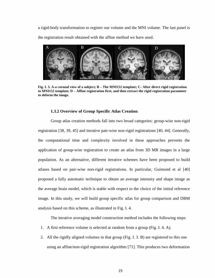
Fig. I. 3 illustrates the process used to register one volume to the MNI template.
The left panel in this figure shows one of our volumes before registration. The second
panel is the MNI atlas. The third panel is the registration result obtained when using only
19
a rigid-body transformation to register our volume and the MNI volume. The last panel is
the registration result obtained with the affine method we have used.
Fig. I. 3. A-a coronal view of a subject; B – The MNI152 template; C- After direct rigid registration
to MNI152 template; D – Affine registration first, and then extract the rigid registration parameter
to deform the image.
1.3.2 Overview of Group Specific Atlas Creation
Group atlas creation methods fall into two broad categories: group-wise non-rigid
registration [38, 39, 45] and iterative pair-wise non-rigid registrations [40, 44]. Generally,
the computational time and complexity involved in these approaches prevents the
application of group-wise registration to create an atlas from 3D MR images in a large
population. As an alternative, different iterative schemes have been proposed to build
atlases based on pair-wise non-rigid registrations. In particular, Guimond et al [40]
proposed a fully automatic technique to obtain an average intensity and shape image as
the average brain model, which is stable with respect to the choice of the initial reference
image. In this study, we will build group specific atlas for group comparison and DBM
analysis based on this scheme, as illustrated in Fig. I. 4.
The iterative averaging model construction method includes the following steps:
1. A first reference volume is selected at random from a group (Fig. I. 4. A).
2. All the rigidly aligned volumes in that group (Fig. I. 3. B) are registered to this one
using an affine/non-rigid registration algorithm [71]. This produces two deformation
A B C D

20
fields for each volume. One, which we call the forward deformation field, registers a
volume to the reference volume. The other, which we call the inverse deformation
field (Fig. I. 3. D), registers the target volume to each volume (see section 1.3.4
below for a discussion on the celebration of the inverse fields).
3. All the volumes are deformed and reformatted using the forward registration fields,
resulting in a series of volume (Fig. I. 3. C) that are similar to the reference volume.
4. All the registered volumes are intensity-averaged (Fig. I. 4. E) and all inverse
deformation fields are averaged (Fig. I. 4. F).
5. The average inverse field (Fig. I. 4. F) is applied to the intensity average (Fig. I. 4. E)
to produce a new intensity and shape averaged volume (Fig. I. 4. G) which becomes
the updated atlas (Fig. I. 4. A).
6. The process is repeated from step 2 until convergence to the group atlas.
Fig. I. 4. Schematic representation of the atlas creation process used in our study
A
B C
D F
E
G
21
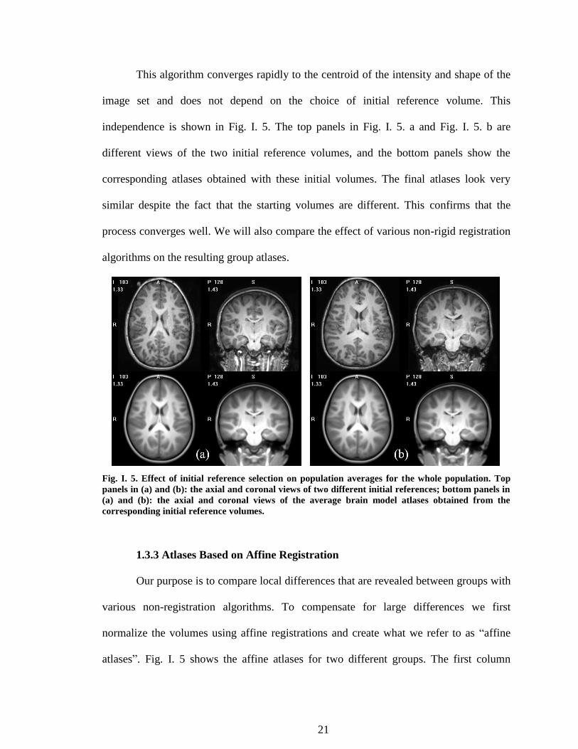
This algorithm converges rapidly to the centroid of the intensity and shape of the
image set and does not depend on the choice of initial reference volume. This
independence is shown in Fig. I. 5. The top panels in Fig. I. 5. a and Fig. I. 5. b are
different views of the two initial reference volumes, and the bottom panels show the
corresponding atlases obtained with these initial volumes. The final atlases look very
similar despite the fact that the starting volumes are different. This confirms that the
process converges well. We will also compare the effect of various non-rigid registration
algorithms on the resulting group atlases.
Fig. I. 5. Effect of initial reference selection on population averages for the whole population. Top
panels in (a) and (b): the axial and coronal views of two different initial references; bottom panels in
(a) and (b): the axial and coronal views of the average brain model atlases obtained from the
corresponding initial reference volumes.
1.3.3 Atlases Based on Affine Registration
Our purpose is to compare local differences that are revealed between groups with
various non-registration algorithms. To compensate for large differences we first
normalize the volumes using affine registrations and create what we refer to as “affine
atlases”. Fig. I. 5 shows the affine atlases for two different groups. The first column

22
shows the initial reference volumes in each group, the second column shows the averaged
intensity volume after the first iteration, and the third column shows the deformed
volumes in column 2 after applying the average inverse deformation field. The fourth and
fifth columns are the deformed atlas results after the second and third iterations. The
affine atlases are blurry, but converge only after two iterations. One image is then
affinely registered to the affine atlas. All the other images are then registered to the
resulting volume with affine transformations. The transformed images are then used as
input for the creation of non-rigid atlases and the subsequent non-rigid registration
processes.
Fig. I. 6. The affine atlases for two different groups. The first column shows the reference volumes in
each group, the second column shows the averaged image after the first iteration The third column
shows the atlases shown in column two deformed with the averaged inverse deformation fields. The
fourth and fifth columns show the affine atlases after the second and third iterations.
1.3.4 Atlases Based on Non-rigid Registrations
As has been discussed in section 1.3.2, the atlas creation process requires the
forward deformed images and the inverse deformation fields to iterate. Computing the

23
inverse deformation field from the forward deformation field or vice-versa is easily done
in the case of a rigid or affine transformation, i.e., in the case of transformations that can
be expressed in terms of a few parameters. It is much more difficult to do for typical non-
rigid transformations, which have thousands of degrees of freedom. Because non-
registration algorithms are typically not symmetric, computing the two fields by
swapping the role of the image volumes (i.e., the target becomes the source and the
source the target) is also not appropriate. Developers of some of the algorithms that we
used provide utilities that permit computing the inverse deformation fields from the
forward deformation fields, but not all of them do. Even when these utilities are provided,
several steps are often required to use them. Furthermore, the formats in which the
deformation fields are stored differ from algorithm to algorithm. There is thus a
substantial amount of data manipulation and processing that needs to be done before
group atlases can be computed and deformation fields compared.
Forward
Images
Forward
deformation
fields
Backward
Images
Backward
deformation
fields
Config.
File
needed?
ABA
(cspline) yes
IRTK
(nreg) call IRTK
transformation1
call IRTK
dof2image2
call IRTK
transformation3
call FSL
invwarp4
yes
ART
(3dwarper) 5
call ART
applywarp3d
call ART
ivf6
no
FSL
(fnirt) call FSL
applywarp
call FSL
fnirtfileutils
call FSL
applywarp
call FSL
invwarp7
yes
SPM (normalisation)
call SPM
Deformations8
call SPM
Deformations8
call SPM
Deformations8 no
Table. I. 1. Comparison of non-rigid registration methods in terms of their outputs for atlas creation
Note:
1: The forward deformed images are Big-Endian. They need to be converted to Little-Endian.

24
2. The results are three separate deformation fields in X, Y and Z directions. The Y direction
needs to be multiplied by (-1) to correspond to the convention used by the other algorithms.
3. Needs a specification of “-v” in the transformation to obtain the inverse deformed image, it
takes about one hour to do. The inverse deformation fields are not exported. There is no
mechanism provided by the IRTK developers to get access to the inverse fields.
4. Since there is no “easy” way to invert the forward deformation fields with IRTK tools, we need
to modify the format of the forward DF to make it a suitable input for the FSL tool invwarp,
which takes about 1.5 hour. We compared the inverse images obtained that way with those
obtained directly with IRTK and we have shown that they are the same.
5. The ART deformation field is in the NIFTI format, a factor called scale_slope needs to be
found in the header and used to multiply the deformation fields to get the real displacement fields.
6. The procedure described in 5 needs to be applied here also.
7. This output needs to be changed from NIFTI_GZ, to NIFTI, and then to ANALYZE format to
deform the averaged image with a software developed in house.
8. In MATLAB, the Deformations module in SPM has different toolboxes for each step.
Table.I.1 below shows what each registration algorithm provides and how things
have been computed when the information is not directly available. The check mark ( )
means that the information is directly obtained from the registration steps, without
additional processing step or format change.
All the non-rigid registrations are done on the Advanced Center for Computing
and Research Education (ACCRE) Linux cluster at Vanderbilt University. To run or call
any program on a cluster, an associated PBS (portable batch system) file is needed to
submit the job. Programs to write and modify PBS files are needed at each step for each
non-rigid registration method. When configuration files are needed, programs to write
and modify the configuration files also need to be written. Most of the averaging
calculations on the forward images and inverse deformation fields are conducted on the
cluster with a C program; additional operations to deform the average image at each
25
iteration are carried out using software developed in house. SPM analysis runs in the
MATLAB environment and batch processes are transferred to the cluster. As discussed
above there are many data format conversions among RAW, ANALYZE, NIFTI, and
NIFTI_GZ formats that are required at various stages and great care needs to be taken to
create header files required by the various packages. Before running algorithms in batch
for all the data, experiments have been conducted to guarantee the correct interpretation
of deformation field format and data format conversions. We have developed a pipeline
integrating all necessary processing steps to run on the ACCRE cluster in parallel for
each of the five non-rigid registration algorithms, permitting processing different dataset
automatically.
1.4 OVERVIEW OF THIS DISSERTATION
Two very different real data sets and a series of simulated datasets are used in our
study. The first real dataset includes both normal control subjects and patients suffering
from the Williams Syndrome (WS). There are large and well-documented anatomical
differences between the normal and WS populations. The second data set contains MR
images acquired from third-grade children with different levels of mathematical ability,
from normal to severe difficulties. Anatomic differences between children with high and
low mathematical scores are not as obvious as those in the first dataset. We are interested in
using both real datasets to compare the effect of non-rigid registration algorithms on DBM
analysis. A series of simulated data sets for which the ground truth is known has also been

26
used in our comparative study. More information about each of these datasets will be found
in the following chapters.
The reminder of this dissertation is organized as follows. Chapter II studies the
effect of non-rigid registration algorithms on DBM results and atlas creation using the
Williams Syndrome dataset. The unique nature of the data set used in this study also
permits the correlation of visible anatomical differences between the groups and regions
of difference detected by each algorithm. Chapter III uses similar techniques to compare
registration’s effect on DBM results with the children dataset. Chapter IV presents the
simulation model and introduces different growth models that have been used as ground
truth to compare DBM results. Chapter V concludes the work presented in this thesis and
outlines possible directions for future work.

27
CHAPTER 2
EFFECT OF NON-RIGID REGISTRATION ALGORITHMS ON
DEFORMATION BASED MORPHOMETRY: A COMPARATIVE STUDY WITH
CONTROL AND WILLIAMS SYNDROME SUBJECTS
2.1 INTRODUCTION
Non-rigid registration is a core component in many medical image analysis
processes. Typical applications include spatial normalization, atlas-based segmentation,
and deformation-based morphometry (DBM). Atlas-based segmentation refers to a
technique in which structures of interest are first delineated in one or several reference
image volumes. These reference volumes, also called atlases are registered to a new
volume, often called the target volume, and the registration transformation is used to
transfer labels from the atlases to the target volume. If the registration is accurate,
accurate segmentation can thus be obtained. DBM commonly refers to a set of techniques
in which features extracted from the deformation fields computed with non-rigid
registration algorithms are used to detect differences between groups [7, 8, 57]. It is an
alternative to the more widespread voxel-based morphometry (VBM) techniques [47].
Over the last five to ten years, a number of non-rigid registration algorithms have
been proposed but their comparison and evaluation is a difficult task. As opposed to
rigid-body problems for which a ground truth can be established and used to measure
registration accuracy [35], evaluation of algorithms designed for non-rigid registration
28
remains somewhat empirical. Several approaches have been proposed, and studies have
compared these algorithms using metrics such as tissue overlap measures [32, 36, 37, 65]
or dispersion of homologous landmarks [28]. Recently, Klein et al. [33]conducted what
is the most comprehensive study we are aware of in which 14 algorithms are compared
using tissue overlap measures. However, evaluating the effect of non-rigid registration
algorithms on DBM-derived findings remains largely unaddressed. One exception is the
work of Yanovsky et al. [66] in which the power and stability of large-deformation
registration schemes combined with various matching functionals were studied with
tensor-based morphometry.
The goal of this work is to determine the sensitivity of DBM-based findings to the
non-rigid registration algorithms used to conduct the DBM study. To avoid the bias
introduced by a single subject in DBM analysis, a group template with average anatomy
is usually created [9, 21, 72] as the DBM atlas to which all volumes are subsequently
registered. We thus begin by investigating whether or not the choice of a particular non-
rigid registration algorithm affects the creation of this group atlas. We then perform DBM
analysis using five different non-rigid registration algorithms to detect regional
differences between two groups. To do so we use two metrics, one is sensitive to
volumetric differences, the other to anatomic variability. A major difficulty with
comparative DBM studies is the lack of ground truth. One unique feature of this study is
that we have used samples from populations for which detailed anatomical differences
have previously been studied and reported. We show that our group atlases preserve these
characteristics. We can thus relate DBM findings to visible anatomical differences in
these atlases. The remainder of this chapter is organized as follows: In the next section,

29
we describe the data and methodology we have used. Section 2.3 reports our results. Our
conclusions are presented in section 2.4.
2.2 MATERIALS AND METHODS
2.2.1 Data and Preprocessing
Our study was conducted on a set of 26 subjects. Thirteen of these (8 males, 5
females; mean age, 23.6±4.2 years) were subjects with Williams Syndrome (WS) and
thirteen were age-matched typically-developing Normal Control (NC) subjects (7 males,
6 females; mean age, 23.1±5.8 years). Williams Syndrome is a rare genetic disorder
caused by the deletion of approximately 25 genes in the 7q11.23 region of the genome
[73, 74]. WS subjects have mild to moderate intellectual disability and particular deficits
in visual-spatial skills, but they also display unique behavioral features such as
hypersociability, hyperaffiliative behaviors, atypical, highly expressive language and
enhanced fascination with music [75]. There are well-documented anatomical differences
between NC and WS subjects, including decreased overall brain and cerebral volumes[21,
73], differences in corpus callosum shape [76], shortened dorsal end of the central sulcus
[77, 78], anomalous sylvian fissure morphometry [79], enlarged cerebellar vermis [80],
and a bilateral reduction in anterior and posterior insular volume [81].
Images were acquired with a 3T Philips Achieva MRI scanner with an 8-channel
receiver head coil and 40 mT/m gradients (200mT/m/ms slew-rate). For each subject, a
3D T1-weighted anatomic volume was obtained with a turbo field echo (TFE) sequence
with matrix size of 256 x 256 x 170 and voxel size of 1 mm3. All scans were acquired at

30
the Vanderbilt University Institute of Imaging Science. All scans were corrected for
intensity non-uniformity using the N3 algorithm [69]. To orient all the volumes in a
standard pose, one of the volumes was registered to the MNI template [70]. This was
done by registering one volume to the MNI atlas with a nine-parameter transformation
and then using the rigid body component of the transformation. (This was done because
differences in head coverage and head size did not permit accurate registration with only
a rigid body transformation.) All the other volumes were then registered to this first one
using a rigid-body transformation computed with a standard intensity based registration
algorithm [71]. Normalized Mutual Information (NMI) was used as similarity measure
[67]. All the computations in this study were carried out on the Advanced Computing
Center for Research and Education (ACCRE) cluster at Vanderbilt University.
2.2.2 Creation of Group Atlases
To determine whether or not the choice of registration algorithm affects the shape
of group atlases, we have used each registration algorithm to create two atlases, i.e., one
for the WS group and the other for the NC group. This was done also to determine the
extent to which group atlases would capture anatomic differences that have been
documented previously. A number of procedures have been reported in the literature to
create group atlases [40, 82-84]. We have selected a widely used iterative method put
forth by Guimond et al. [40]. For a group of image volumes, one volume is first
randomly chosen as an initial atlas to which all the other volumes in the dataset are
registered. The forward (i.e., from the subjects to the atlas) and the backward (i.e., from
the atlas to the subjects) deformation fields are computed. As will be discussed further,

31
some registration algorithms produce both fields when others require additional
computations to obtain one from the other. The subject images are deformed with the
forward fields and intensity averaged. The average of the backward fields is then applied
to this intensity average to produce an updated group atlas. The registration and
averaging processes are repeated until convergence, which is typically achieved after
three or four iterations.
The group atlas was created in two steps. First, one WS volume and one NC
volume were selected to initialize an affine atlas creation process. One affine WS atlas
and one affine NC atlas were computed with only affine transformations to mitigate the
potential bias introduced by the starting volumes. Then all the volumes were registered to
their respective affine atlas with nine-parameter affine registrations adjusting for the
brain size differences. Second, one of the affinely registered volumes was randomly
selected within each group as initial volume for the iterative creation of the non-rigid
atlases. The non-rigid atlases were computed with each of the five non-rigid registration
techniques used in this study (these algorithms are described below). Overall ten atlases
based on non-rigid registration algorithms were thus computed, five WS and five NC.
To investigate the impact of registration algorithms on DBM results, one single
DBM atlas had to be produced. This was done as described above except that all the
volumes were pooled together. This process started with the calculation of an overall
affine atlas and all the 26 volumes were affinely registered to this overall affine atlas.
Then an overall average intensity and shape volume, called the DBM atlas, was
computed. As will be shown in section 2.3.1, the choice of non-rigid registration
algorithm has little impact on the creation of atlases. The overall DBM atlas was thus

32
created with one single non-rigid registration algorithm. The Adaptive Bases Algorithm
(ABA) [26] that was developed in-house and described below has been used for this
purpose. Once the overall DBM atlas was computed, five non-rigid registration
algorithms were used to calculate the non-rigid transformations that register the 26
affinely registered volumes to this DBM atlas. For each registration algorithm, we thus
produced 26 deformation fields; these were then analyzed and compared.
2.2.3 Non-rigid Registration Algorithms
We selected five well-established non-rigid registration algorithms for
comparison: 1) the Image Registration Toolkit (IRTK) [27]; 2) the FMRIB Nonlinear
Image Registration Tool (FSL) [64]; 3) the Automatic Registration Tools (ART) [28]; 4)
the Adaptive Bases Algorithm (ABA) [26]; 5) SPM normalization[29]. IRTK and ART
were among the best-ranked registration algorithms in Klein’s study [33]. We added
ABA because we have considerable experience with its use, as well as FSL and SPM that
are widely used. Each algorithm is described briefly in the following subsections. Each
algorithm outputs deformation fields in a different format and some but not all generate
both the forward and the backward fields. Techniques that were used to obtain these are
detailed below.
2.2.3.1 IRTK
IRTK uses the Normalized Mutual Information (NMI) [67] as the image
similarity measure to maximize [27]. The deformation field is modeled as a linear
combination of 3D B-splines. The executable for IRTK nreg can be downloaded from:
http://www.doc.ic.ac.uk/~dr/software. Utilities are provided to generate the forward
33
deformed images and the associated deformation fields. There is no utility provided to
produce the inverse deformation field. In this study, we have generated these fields with
the FSL inwarp facility. This required modifying the format of the forward deformation
fields produced by IRTK to make them compatible with inwarp.
2.2.3.2 FSL
The FSL non-linear image registration (FNIRT) tool is included in the FMRIB
Software Library (FSL) (http://www.fmrib.ox.ac.uk/fsl/). The deformation field is
modeled as a linear combination of basis functions that can be quadratic or cubic B-
splines. The similarity measure is the sum-of-square differences between the images. The
algorithm produces a series of coefficients that can be used to produce the deformed
images with a utility called applywarp. The forward and reverse deformation fields are
obtained with the utilities fnirtfileutils and invwarp, respectively.
2.2.3.3 ART
The Automatic Registration Toolbox (ART) is a non-parametric method [28] that
maximizes the local cross-correlation between the two images. The ART tool can be
found at NITRC: http://www.nitrc.org/projects/art/. The 3dwrapper utility generates the
deformed images and forward deformation fields. Computing the inverse deformation
fields requires an additional step performed with the utility ivf. Both the forward and
inverse deformation fields are in the NIFTI format. As such, the real displacement fields
need to be computed from those stored in the file using a scale factor called scale_slope
that is found in the file header.
2.2.3.4 ABA

34
The ABA algorithm [26] models the deformation field as a linear combination of
radial basis functions and optimizes the normalized mutual information between two
images. The ABA executable cspline generates the forward and inverse deformed image
and deformation fields automatically. The forward and inverse deformation fields are
constrained to be inverses of each other.
2.2.3.5 SPM
The normalization utility in SPM8 is an algorithm that minimizes the mean square
differences between a template and a warped source image using a deformation field
generated with a linear combination of about 1000 low frequency three-dimensional
cosine bases [29]. The forward and inverse deformation fields can be obtained with the
Deformations Toolbox in SPM8.
2.2.4 Features Used in our DBM Analysis
We have used two features estimated from the deformation fields to perform our
DBM analysis: the Jacobian determinant of the transformation and the magnitude of the
local displacement.
Jacobian determinant: The Jacobian determinant (referred to as JAC in the
remainder of this article) of a 3D transformation is defined as follows:
( ) |
( ) ⁄ ( ) ⁄ ( ) ⁄
( ) ⁄ ( ) ⁄ ( ) ⁄
( ) ⁄ ( ) ⁄ ( ) ⁄| (21)
in which the vector is the vector of displacements at position (x,y,z).
The JAC measures local volume changes. Values greater than one indicate tissue
expansion and values smaller than one indicate tissue compression. A value of one

35
indicates no volume change. It is a measure that is commonly used in DBM-based studies
[3, 16-18, 21, 57].
Magnitude of the deformation field: The magnitude of the deformation field
(referred to as DFM in the reminder of this chapter) is defined as follows:
( ) √ (22)
The DFM has been used [8, 9, 84, 85] as a measure of variability in a set of image
volumes. If all the volumes in a set were exactly identical, the group atlas would be
identical to the volumes, and the magnitude of the deformation field would be zero. The
larger the difference between volumes the larger their “distance” from the atlas volume
and the larger the displacement needed to register a particular volume to this atlas.
2.2.5 Statistical Analysis
Statistical comparison of JAC and DFM across groups was carried out using the
general linear model regression implemented in SPM8. For each registration algorithm,
two sample voxel-wise t-tests were computed between the NC subjects and the WS
subjects, leading to one T map for each of the two DBM features. Family Wise Error
(FWE) corrections based on the random field theory [86] was performed to address the
multiple comparison issues at both peak and cluster level inferences. Peak-level
correction allows focal differences between groups to be identified while cluster-level
correction reveals more diffuse differences. In all the results presented in this study an
uncorrected p value of 0.001 was used to threshold the T maps (T > 3.47, df =24). A
corrected p value of 0.05 was used as the significance threshold at both peak and cluster

36
levels. Clusters that survived after either peak or cluster level correction were deemed
statistically significant.
2.2.6 Comparisons of DBM Results
Every registration algorithm used in this study produced statistically significant
clusters. However, the number, size, and position of these clusters varied across
algorithms. Thus, comparing these algorithms is difficult. Even answering the simple
question “Are these algorithms detecting equivalent regions of interest?” is complicated
because regions produced by several algorithms may overlap partially or several small
regions produced by one algorithm may overlap with a single larger region produced by
another algorithm. To address this
issue, we have developed the
following scheme. First, for each
algorithm, binary images were
produced in which a voxel value
equals one if the voxel is within a
significant cluster and zero otherwise.
This is illustrated schematically in Fig.
II.1 for three registration algorithms.
Then these binary images were added together, producing an image in which voxel
values range from zero to N with N the number of registration algorithms. We call this
image the membership map and it is shown on the bottom left of Fig. II.1. Here, values in
the membership map range from 0 to 3 and voxels are color-coded to reflect this (1 =
Fig. II. 1. Region selection for DBM results comparison.

37
blue, 2 = green, 3 = red). This membership map has three connected regions R1, R2, and
R3. Regions in the membership maps are then filtered using a membership value
threshold. In the example shown in Fig. II. 1, regions that do not contain voxels with a
value of 3 are eliminated. The final region of interest is defined as the union of the binary
masks that overlap the connected region that contains voxels with a value of 3. Following
the example illustrated in Fig. II. 1, the rectangular regions produced by algorithms A and
B and the two small bottom regions produced by algorithm C would be considered to be
the equivalent region across algorithms. In our study, we compare five algorithms and we
use a membership threshold of 4 to select regions of interest.
Our analysis is performed in DBM atlas space, so the localization of the
statistically significant clusters is not based on standard Talairach coordinates. Instead the
names of the regions are obtained by visual comparisons of our DBM clusters with
labeled MR images using two apps for the iPhone: the iSurf Brainview v3.0.0
(http://itunes.apple.com/app/isurf-brainview/id381072423?mt=8, Netfilter, Rio de Janeiro,
Brazil) based on the MRI automatic segmentation produced by FreeSurfer and the Brain
Tutor 3D (http://www.brainvoyager.com/iOS/iphonebraintutor3d.htm).
2.3 RESULTS
2.3.1 Effects of Registrations on Group Atlas
Fig. II. 2 presents ten group atlases that have been produced using the method
described in section 2.2.2. Each column shows the NC atlases (top), the WS atlases
(middle), and the difference between the two (bottom) for each of the five algorithms

38
used herein. Qualitatively, there is little difference between the atlases except that the
volumes produced by SPM are slightly blurrier. The difference volumes show that
anatomic differences highlighted by ABA, IRTK, FSL, and ART are largely similar. One
obvious difference is that the NC atlases are larger in size than the WS atlases; this is in
accordance with what has been reported in the literature[73].
Fig. II. 2. The creation of group atlases for the NC (top panel) and the WS (middle panel) group
using five registration algorithms (from left to right): ABA, IRTK, FSL, ART, SPM. The image
differences are shown at the bottom.
It has also been documented [77, 78] that WS subjects have shorter central sulci
that do not come as close to the inter-hemispheric line as those in control subjects. These
studies were performed manually on individual scans. Fig. II. 3 shows cortical renderings
of the group atlases in which the central sulcus has been delineated (red lines for the NC
group and green lines for the WS group). This figure shows that the group atlases
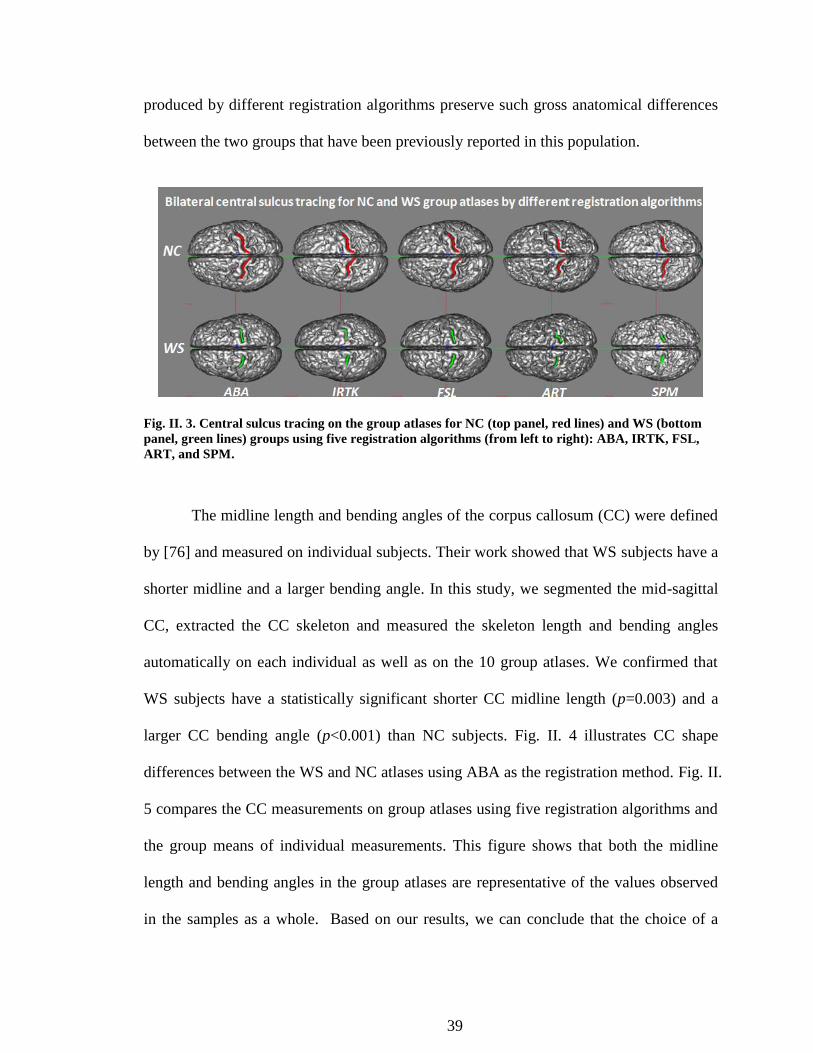
39
produced by different registration algorithms preserve such gross anatomical differences
between the two groups that have been previously reported in this population.
Fig. II. 3. Central sulcus tracing on the group atlases for NC (top panel, red lines) and WS (bottom
panel, green lines) groups using five registration algorithms (from left to right): ABA, IRTK, FSL,
ART, and SPM.
The midline length and bending angles of the corpus callosum (CC) were defined
by [76] and measured on individual subjects. Their work showed that WS subjects have a
shorter midline and a larger bending angle. In this study, we segmented the mid-sagittal
CC, extracted the CC skeleton and measured the skeleton length and bending angles
automatically on each individual as well as on the 10 group atlases. We confirmed that
WS subjects have a statistically significant shorter CC midline length (p=0.003) and a
larger CC bending angle (p<0.001) than NC subjects. Fig. II. 4 illustrates CC shape
differences between the WS and NC atlases using ABA as the registration method. Fig. II.
5 compares the CC measurements on group atlases using five registration algorithms and
the group means of individual measurements. This figure shows that both the midline
length and bending angles in the group atlases are representative of the values observed
in the samples as a whole. Based on our results, we can conclude that the choice of a

40
particular registration algorithm has
little effect on the resulting group
atlases at both the cortical and deep
brain structure levels. To simplify
our analysis of DBM results, we have thus used a single algorithm to produce an overall
DBM atlas based on the pooled WS and NC volumes. We have chosen ABA to do so
because we are most familiar with this algorithm.
Fig. II. 5. Effect of registration on Corpus Callosum (CC) shape differences for NC and WS atlases.
2.3.2 Raw T maps
Fig. II. 6 shows the raw T maps that have been obtained with the five algorithms
(columns) for both the JAC and DFM features (rows). In this figure, warm colors indicate
that the feature values are larger for the NC subjects than the WS subjects; cold colors
mean the opposite. A number of observations can be made from these images. First,
general patterns are somewhat similar across algorithms except for SPM. Second, the
smoothness of the maps varies across algorithm. This variation in smoothness is related
to the variation in smoothness of the deformation fields, and it is more pronounced for the
JAC than the DFM because the former is based on the derivative of the fields. These
figures show that ART produces the least smooth T-maps. ABA comes second, followed
by FSL and then IRTK.
Fig. II. 4. CC shape differences between NC and WS.

41
Fig. II. 6. T maps for JAC (top row) and DFM (bottom row) obtained with different registration
algorithms.
Fig. II. 7. Smoothness estimation (FWHM in X, Y and Z directions) for JAC and DFM T maps for
different registration algorithms (from left to right): ABA, IRTK, FSL, ART, and SPM.
We have used the SPM8 utility to estimate the smoothness of the JAC and DFM
map expressed as full width at half maximum (FWHM) in the X, Y, and Z directions.
These values, which are shown in Fig. II. 7, are used to calculate FWE corrected p values
using the Random Field Theory [86]. Based on these results, one could anticipate that
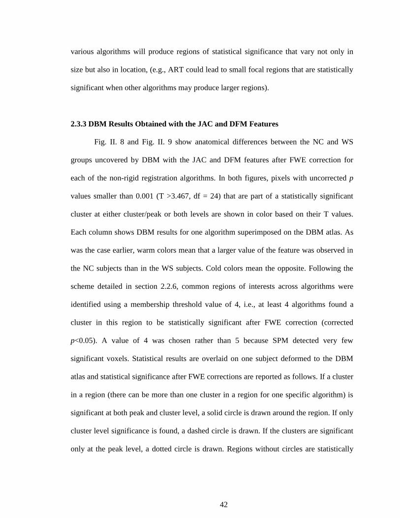
42
various algorithms will produce regions of statistical significance that vary not only in
size but also in location, (e.g., ART could lead to small focal regions that are statistically
significant when other algorithms may produce larger regions).
2.3.3 DBM Results Obtained with the JAC and DFM Features
Fig. II. 8 and Fig. II. 9 show anatomical differences between the NC and WS
groups uncovered by DBM with the JAC and DFM features after FWE correction for
each of the non-rigid registration algorithms. In both figures, pixels with uncorrected p
values smaller than 0.001 (T >3.467, df = 24) that are part of a statistically significant
cluster at either cluster/peak or both levels are shown in color based on their T values.
Each column shows DBM results for one algorithm superimposed on the DBM atlas. As
was the case earlier, warm colors mean that a larger value of the feature was observed in
the NC subjects than in the WS subjects. Cold colors mean the opposite. Following the
scheme detailed in section 2.2.6, common regions of interests across algorithms were
identified using a membership threshold value of 4, i.e., at least 4 algorithms found a
cluster in this region to be statistically significant after FWE correction (corrected
p<0.05). A value of 4 was chosen rather than 5 because SPM detected very few
significant voxels. Statistical results are overlaid on one subject deformed to the DBM
atlas and statistical significance after FWE corrections are reported as follows. If a cluster
in a region (there can be more than one cluster in a region for one specific algorithm) is
significant at both peak and cluster level, a solid circle is drawn around the region. If only
cluster level significance is found, a dashed circle is drawn. If the clusters are significant
only at the peak level, a dotted circle is drawn. Regions without circles are statistically

43
significant regions at either peak/cluster level or both levels after FWE corrections that
are found by less than four algorithms.
Three consistent regions of interests (ROIs) were found when the JAC feature is
used. Two of them (R1 and R2) indicate volumetric enlargement in the NC subjects
localized bilaterally around the insular cortex, Sylvian fissure, putamen, pallidum, and
some white matter. R3 is localized in the center of the cerebellum and suggests that WS
subjects show an enlargement of the cerebellum. These ROIs were found by DBM with
ABA, IRTK, FSL, and ART. The DBM results based on the SPM normalization are
qualitatively and quantitatively different. This algorithm only finds one large region
located in the frontal lobe that is significant at both peak and cluster levels.
There are also a number of other statistically significant clusters found by less
than four algorithms (see Fig. II. 8). ABA found a cluster around the anterior cingulate
cortex close to the genu of the CC showing volumetric enlargement for NC subjects.
ABA, IRTK and FSL all found clusters around the middle of the corpus callosum that
indicate volumetric enlargement for NC subjects. FSL and ART found volumetric
reduction for NC subjects around the splenium of the CC. These clusters are likely
caused by differences in shape in the CC between NC and WS groups. ABA, IRTK, FSL
and ART all found different clusters in the brain stem, but these regions do not overlap.
FSL also found one cluster around the posterior part of the superior frontal sulcus
showing a volumetric reduction in NC subjects.
Two consistent regions of interests (R1 and R2) were found when using the DFM
feature. ABA, IRTK, FSL, and ART found clusters significant after peak level and/or
cluster level correction bilaterally across the insular cortex, orbitofrontal gyrus and

44
temporal pole (see Fig. II. 9). These blue patches indicate more anatomical variations in
WS subjects than in NC subjects, though the size and distribution of clusters vary across
algorithms. SPM also found a cluster in R1 with an uncorrected p of 0.001, but this
region was not significant after FWE correction (not shown). FSL found two other unique
clusters around the left superior frontal gyrus (significant at both levels) and left inferior
frontal gyrus (significant at only cluster level).
Table. II. 1 and Table. II. 2 list all the clusters found in each ROI by different
algorithms and their levels of significance after FWE corrections for the JAC and the
DFM features, respectively. For example, in region 1 in Table. II. 1, ABA found two
clusters significant at the cluster level, IRTK found one contiguous region significant at
both peak and cluster levels, FSL found one contiguous cluster significant at both peak
and cluster levels (note that this cluster is very large and extends across hemispheres; we
separated the voxels in the left and right hemispheres for analysis purpose), and ART
found three isolated clusters all significant at cluster level and two of them are significant
at peak level. The rest of Table. II. 1 and Table. II. 2 can be interpreted in the same way.
The significance information in Table. II. 1 and Table. II. 2 is also reflected in the circle
line types in Fig. II. 8 and Fig. II. 9, respectively.
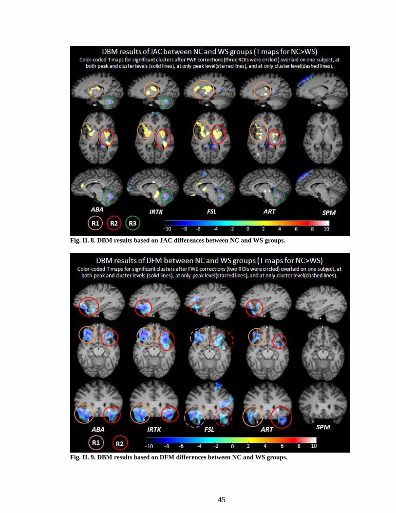
45
Fig. II. 8. DBM results based on JAC differences between NC and WS groups.
Fig. II. 9. DBM results based on DFM differences between NC and WS groups.
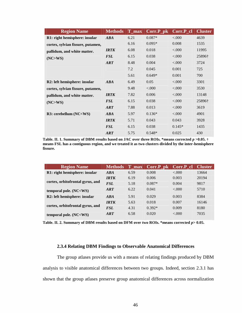
46
Region Name Methods T_max Corr.P_pk Corr.P_cl Cluster
size R1: right hemisphere: insular
cortex, sylvian fissure, putamen,
pallidum, and white matter.
(NC>WS)
ABA 6.21 0.087* <.000 4639
6.16 0.095* 0.008 1535
IRTK 6.08 0.018 <.000 11995
FSL 6.15 0.038 <.000 25896†
ART 8.48 0.004 <.000 3724
7.2 0.045 0.001 725
5.61 0.649* 0.001 700
R2: left hemisphere: insular
cortex, sylvian fissure, putamen,
pallidum, and white matter.
(NC>WS)
ABA 6.49 0.05 <.000 3301
9.48 <.000 <.000 3530
IRTK 7.82 0.006 <.000 13148
FSL 6.15 0.038 <.000 25896†
ART 7.88 0.013 <.000 3619
R3: cerebellum (NC<WS)
ABA 5.97 0.136* <.000 4901
IRTK 5.71 0.043 0.043 3928
FSL 6.15 0.038 0.145* 1435
ART 5.75 0.548* 0.025 430
Table. II. 1. Summary of DBM results based on JAC over three ROIs. *means corrected p >0.05. †
means FSL has a contiguous region, and we treated it as two clusters divided by the inter-hemisphere
fissure.
Region Name Methods T_max Corr.P_pk Corr.P_cl Cluster
Size
R1: right hemisphere: insular
cortex, orbitofrontal gyrus, and
temporal pole. (NC<WS)
ABA 6.59 0.008 <.000 13664
IRTK 6.19 0.006 0.003 20194
FSL 5.18 0.087* 0.004 9817
ART 6.22 0.041 <.000 5710
R2: left hemisphere: insular
cortex, orbitofrontal gyrus, and
temporal pole. (NC<WS)
ABA 5.91 0.029 0.003 8384
IRTK 5.63 0.018 0.007 16146
FSL 4.31 0.392* 0.009 8180
ART 6.58 0.020 <.000 7035
Table. II. 2. Summary of DBM results based on DFM over two ROIs. *means corrected p> 0.05.
2.3.4 Relating DBM Findings to Observable Anatomical Differences
The group atlases provide us with a means of relating findings produced by DBM
analysis to visible anatomical differences between two groups. Indeed, section 2.3.1 has
shown that the group atlases preserve group anatomical differences across normalization

47
algorithms at both cortical and deep brain structure levels. To correct for size differences
between the groups and thus permit observation of local differences between these groups,
the WS and NC group atlases were registered to the DBM atlas with a nine-degree
freedom transformation.
Fig. II. 10. Scheme used for affine registration of group atlases to the DBM atlas (highlight of
observable differences).
Fig. II. 10 shows the process schematically. The top panel shows an axial view in
the NC atlas (left) and the WS atlas (right) obtained with the ABA algorithm. The bottom
panel shows the deformed group atlases (NC on the left and WS on the right) registered
to the DBM atlas (middle) with affine transformations. The horizontal lines have been
drawn on the deformed group atlases (pink for NC and cyan for WS) to show that affine
transformations have compensated for width differences in the atlases. Group differences,
after affine transformations, are clear and highlighted with curved lines drawn on the
deformed group atlases. The anterior end of the right insular cortex (shown with red

48
arrows) extends further in the NC atlas than it does in the WS atlas. On both hemispheres,
there are lateral displacements between the NC and WS groups along the coursing of the
cortical area circumscribed by the sylvian fissure, the superior temporal gyrus and the
inferior insular cortex. Notably, the DBM atlas is somewhere in the middle.
Fig. II. 11 compares visible anatomical differences between groups and regions of
statistically significant differences found by DBM with ABA, IRTK, FSL, and ART. The
top panel shows the zoomed view of the bottom panel in Fig. II. 10 (subpanel A-C), as
well as the color-coded intensity differences between the deformed NC and WS atlases
(subpanel D). The bottom panel displays the DBM results of JAC based on different
registration methods superimposed onto the DBM atlas over region R1 (see Fig. II. 8).
Fig. II. 11. Top panel: A) deformed NC atlas, B) DBM atlas, C) deformed WS atlas, and D) Image
differences between A and C (Colormap range: [-160,160]). Bottom panel: The DBM results for JAC
based on a) ABA, b) IRTK, c) FSL, and d) ART. The pink and cyan lines were drawn on the
deformed NC and WS atlas respectively.
To interpret these results, one needs to keep in mind that all the non-rigid
registration algorithms that have been used in this study are intensity-based. Typically,
these algorithms will be driven by regions of high contrast, i.e., edges in the images. The

49
transformations in regions of low contrast are plausible interpolations whose smoothness
depends on the regularization scheme or the mechanism used by each algorithm to model
the deformation fields. As seen on the top panel figures, a larger area of gray matter is
present in the anterior part of right insular cortex in the NC atlas than in the WS atlas
(marked with red arrows). This is also reflected as a blue blob in subpanel D. Thus, the
DBM atlas had to be expanded in this region to match the NC group and contracted to
match the WS group. The DBM results based on all four algorithms indeed found that the
NC group has a larger volume than the WS group in the right anterior insular cortex.
DBM results also show that this statistically significant different region spans the
putamen, pallidum, and some white matter. Subpanel D does not show obvious
differences between group atlases around the basal ganglia (putamen and pallidum),
however the lateral displacements of the cortical area (shown with yellow arrows)
between the group atlases are apparent. Registration algorithms need to displace this
particular cortical area laterally and medially when matching the DBM atlas to the NC
and WS groups, respectively by stretching or compressing the low-contrast region of the
basal ganglia. DBM results have detected areas of such expansion, whose patterns are a
function of the transformation smoothness (e.g., ART detects several localized regions of
expansion when IRTK detects one single large one).

50
Fig. II. 12. Top panel: A) deformed NC atlas, B) DBM atlas, C) deformed WS atlas, and D) Image
differences between A and C (Colormap range: [-160,160]). Bottom panel: The DBM results for JAC
based on a) ABA, b) IRTK, c) FSL, and d) ART. The pink and cyan lines were drawn on the
deformed NC and WS atlas respectively
Fig. II. 12 compares the cerebella in the WS and the NC atlases after these have
been registered to the DBM atlas with a nine-degree freedom transformation. The
cerebellum contours have been drawn in pink on the deformed NC atlas and in cyan on
the deformed WS atlas, showing that the cerebellum is larger in the WS group than it is in
the NC group after adjusting for brain size differences. It also shows that the lobes are
better separated in the NC atlas than in the WS atlas. In the bottom panel, colored clusters
of statistically significant differences between JAC values in the NC and WS groups are
superimposed on the DBM atlas. Here, the algorithms had to expand the cerebellum in
the DBM atlas to make it match the cerebellum in the WS group and compress it to make
it match the cerebellum in the NC group. The blue patches reflect JAC values larger for
the WS group than the NC group. Smoothness of the deformation fields computed by
each algorithm influences the location and extent of the patches. The lack of contrast
inside the cerebellum and good contrast with the surrounding CSF explains that ABA,
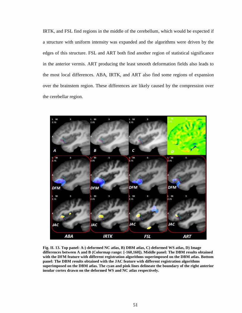
51
IRTK, and FSL find regions in the middle of the cerebellum, which would be expected if
a structure with uniform intensity was expanded and the algorithms were driven by the
edges of this structure. FSL and ART both find another region of statistical significance
in the anterior vermis. ART producing the least smooth deformation fields also leads to
the most local differences. ABA, IRTK, and ART also find some regions of expansion
over the brainstem region. These differences are likely caused by the compression over
the cerebellar region.
Fig. II. 13. Top panel: A:) deformed NC atlas, B) DBM atlas, C) deformed WS atlas, D) Image
differences between A and B (Colormap range: [-160,160]). Middle panel: The DBM results obtained
with the DFM feature with different registration algorithms superimposed on the DBM atlas. Bottom
panel: The DBM results obtained with the JAC feature with different registration algorithms
superimposed on the DBM atlas. The cyan and pink lines delineate the boundary of the right anterior
insular cortex drawn on the deformed WS and NC atlas respectively.
52
Fig. II. 13 relates observable group differences with the DBM results obtained
with both the DFM and the JAC features with the different registration algorithms. The
top panel shows a sagittal view of the atlases that cover a sub-region of the right anterior
insular cortex, the only region over which statistically significant differences are found
with both the DFM and JAC features. Pink and cyan lines were drawn to highlight the
boundary of the anterior right insular sulcus on the deformed NC and WS atlases
respectively, showing that the two groups have distinct sulcal patterns around this area.
The middle panel shows areas of statistical significance obtained with the DFM feature
over this region for all registration algorithms. These results indicate that the WS group
has more anatomical variation around the anterior insular cortex, the orbitofrontal gyrus
and the temporal pole than the control group. The bottom panels show the regions of
statistical significance when the JAC feature is used. These results indicate a region of
enlargement around the right anterior insular sulcus in NC subjects. DBM results
obtained with the DFM and JAC features thus indicate that there are more anatomical
variations and a volumetric reduction around the anterior portion of the insular cortex in
the WS group compared to the NC group.
2.4 DISCUSSION
We have used five different non-rigid registration algorithms (ABA, IRTK, FSL,
ART and SPM) to study the effect of registration on atlas creation and on results
produced by DBM analysis. We have shown that the choice of a particular registration
algorithm has little effect on the creation of group atlases. Using data sets acquired from
population samples with documented anatomical differences, we have also shown that all

53
the algorithms we have studied as well as the method used to produce the atlases preserve
anatomical differences between groups at both cortical and deep brain structure levels.
Previous work on structural differences in WS samples relies on volumetric measurement
and shape delineation performed manually or semi-automatically on individual subjects.
Most of these measurements were carried out on two data sets acquired by Reiss and
colleagues [73, 76, 77] and by Jackowski and colleagues [78]. Differences observed
between our group atlases correlate well with these findings. This indicates both that
morphological characteristics of WS brains are stable across samples and that group
atlases that capture these characteristics can be created automatically.
The effects of non-rigid registration algorithms on DBM analysis using both the
JAC and the DFM features were compared both qualitatively and quantitatively using
voxel-wise regression analysis. All the algorithms we studied except for SPM produce
generally similar T maps. After FWE corrections at both peak and cluster level inferences
(uncorrected p<0.001; corrected p<0.05), different registration methods generate
statistically significant clusters that are different, both in terms of size and location. This
is more pronounced for the JAC than the DFM feature. These differences can be
explained, in part, by the smoothness of the deformation fields produced by each
algorithm and the similarity measure used to drive the algorithms.
ABA and IRTK both maximize the normalized mutual information between the
images and both model the deformation field with spline-like basis functions. There is
more agreement between these two algorithms than between other pairs of algorithms.
FSL also models the deformation field with spline functions but uses the intensity
difference between the images as its similarity measure. This may explain several unique

54
clusters found around the cortical area by this algorithm. ART leads to smaller and more
scattered clusters compared to the other algorithms. This is because this algorithm
optimizes a local similarity metric in a non-parametric fashion. It may permit the
detection of small structural differences but our results suggest that it leads to regions that
are artificially broken into several small pieces. Even though the normalization utility in
SPM is widely available and easy to use, our results show that it is not the best approach
to use when performing DBM studies due to the relative low number of degrees of
freedom in the modeling of the deformation fields.
Our study shows that DBM results need to be interpreted with care and that the
characteristics of the registration algorithm used in the study need to be taken into
consideration in the interpretation process. For instance, DBM results obtained with the
JAC show that the NC group has higher JAC values around the anterior insular cortex
and the basal ganglia (putamen and pallidum) than the WS group. Without looking at the
anatomic group atlases we have generated, one may be tempted to conclude that the
relative volumes of the anterior insular cortex, putamen and pallidum are larger in the NC
group than they are in the WS group. Another Jacobian-based morphometry study [22]
performed with the ANIMAL [87] registration algorithm concluded that WS subjects
have disproportionally decreased volumes around the basal ganglia and the thalamus.
However, drawing such conclusion from JAC differences in DBM results alone is not
prudent. Indeed, as was discussed earlier, the group atlases show obvious bilateral
displacements of the sulcus regions surrounding the inferior insular sulcus, sylvian fissure,
and superior temporal gyrus as well as differences in the anterior part of the insular
cortex (Fig. II. 11). Previous work showed anomalous sulcal and gyral morphometry in

55
the sylvian fissure [79] as well as increased cortical thickness around the right perisylvian
area in a WS sample [88]. Cohen et al. [81] measured the morphometry of the insular
cortex on individual subjects and found that both the anterior and posterior insular
volume were reduced bilaterally after accounting for reduced total brain volumes in WS
subjects. Our DBM results reveal consistent findings for the anterior insular cortex, and
the group atlases also showed a more anterior orientation of the anterior insular sulcus in
the NC atlas than that in the WS atlas (Fig. II. 13). However, there is a lack of contrast
around the basal ganglia (the putamen and the pallidum), where the deformation is thus
somewhat arbitrary and a function of the normalization scheme used in the non-rigid
registration algorithm. Thus, it is possible that apparent volume differences in these
regions are caused by displacements driven by the cortical areas. To the best of our
knowledge no measurement of the putamen and pallidum have been made in individual
subjects. We thus cannot verify that areas of statistical differences detected by DBM in
these regions are real.
Results obtained over the cerebellar area also show that drawing very specific
conclusions on group differences based on DBM analysis alone is difficult. ABA, IRTK,
FSL, and ART all find differences in this region but little can be said except that the
overall volume of the cerebellum is larger in the WS group than in the NC group. Schmitt
et al. [80] examined the cerebellar vermis on 20 subjects with WS and 20 age and gender
matched NC subjects, showing that the posterior vermis is significantly larger in WS. Our
JAC-based DBM results only found differences in the center of the cerebellum showing
that the algorithms we have compared can only detect gross volumetric changes over the
cerebellum and not substructure differences.

56
Although not used as often as the JAC, the magnitude of the deformation field
(DFM) may be a useful feature to use to find anatomical variation differences in groups
that cannot be detected by an approach that is only sensitive to volumetric changes. All
registration algorithms except for SPM detect more anatomical variations in WS subject
around the anterior insular cortex and orbitofrontal gyrus in both hemispheres using the
DFM. Several VBM studies have shown bilateral differences in gray matter density
around the orbitofrontal area [79, 89, 90], which may be related to our findings. Also,
surface-based analysis performed on cortical folding showed that the WS subjects have
generally shallower olfactory sulcus compared to NC subjects [91]. However, we do not
know of any work that has compared anatomical variability in WS and control samples,
so we cannot relate our findings to previous reports. Our results suggest that a detailed
analysis of this general orbitofrontal area may reveal other differences between NC and
WS subjects.
In conclusion, to the best of our knowledge, this study is the largest to date that
compares DBM results obtained with various well-established registration schemes. The
subjects on which this study has been conducted permits comparison of DBM findings to
observable anatomical differences, thus providing us with a good ground truth surrogate.
Our study shows that the effect of non-rigid registration algorithms on the creation of
atlases is negligible, meaning that all the algorithms we have evaluated are able to
produce warped images that look alike with the exception of SPM that produces slightly
more blurred images because of the smoothness of the deformation field it produces.
Comparing differences between the group atlases with previously published results, we
can conclude that our atlases are representative of their respective group. But our study

57
also shows that registration algorithms have a substantial effect on DBM results both
qualitatively and quantitatively. Even though general trends are similar across algorithms,
specific conclusions that may be drawn when using one algorithm versus the other may
vary substantially. When performing DBM analysis, our suggestion would thus be to use
more than one algorithm and to look for regions that are consistently labeled as
significant across these algorithms. Interpretation of the DBM results also requires taking
into consideration the location of the detected regions of compression or extension, e.g.,
in a region of high or low contrast, the way the algorithms operate and the properties of
the deformation field. While DBM results based on DFM and JAC can be used as good
screening tools to identify differences between groups, specific conclusions on the nature
and the location of these differences should only be drawn after careful analysis and
possibly after correlating these findings with other biological or behavioral measurements.

58
CHAPTER 3
RELATION BETWEEN CORTICAL ARCHITECTURE AND MATHEMATICAL
ABILITY IN CHILDREN: A DBM STUDY
3.1 INTRODUCTION
The ability to comprehend and manipulate numbers are fundamental cognitive
skills, yet population-based studies indicate that between 5 and 9 percent of U.S. children
exhibit significant deficits in mathematical reasoning, which are manifested as learning
disabilities or difficulties in developing age-appropriate competencies in math. Even as
early as first grade, children with math difficulties (MD) demonstrate a specific weakness
in the ability to accurately and quickly retrieve mathematical facts to perform simple
arithmetic [92, 93], yet little is understood about the origins of such specific difficulties in
the absence of more general limitations on learning and intelligence.
Functional neuroimaging techniques such as functional magnetic resonance
imaging (fMRI) have demonstrated that a reproducible set of parietal, prefrontal and
occipitotemporal brain areas are systematically activated when subjects are asked to
perform simple calculations [94-96]. For example, Dehaene et al. showed that exact
calculations usually rely on semantic identification and retrieval of numerical facts from
memory, engaging prefrontal regions, while approximation recruits bilateral areas of the
parietal lobes involved in visual-spatial processing [95]. Similarly, Simon et al.
characterized the functional specialization of calculation-related activations in the

59
intraparietal sulcus [97]. However, although functional neuroimaging has been
extensively applied to the study of populations with math difficulties, to date there have
been few studies that have used high resolution structural MRI to determine whether
there are differences in brain morphology between normal and MD children, and none
have examined whether specific structural variations in the brain are associated with the
level of math skills in children.
In principle, morphological analysis can reveal differences in the underlying
cerebral substrates between normal populations and groups with mathematical difficulties,
independent of any specific functional assessment. For example, Issacs et al. [98] used
voxel-based morphometry (VBM) to demonstrate that impaired calculation ability in
children with very low birth weight could be associated with less gray matter in the left
parietal lobe in this population than in a normal cohort, while Rotzer et al. [99] showed
that developmental dyscalculia was associated with a significantly reduced gray matter
volume in the right intraparietal sulcus, anterior cingulum, the left inferior frontal gyrus,
and the bilateral middle frontal gyri. Molko et al. [100] also found an abnormal length,
depth, and sulcal geometry of the right intraparietal sulcus in girls with dyscalculia
associated with Turner’s syndrome. These studies provide strong evidence for structural
differences in populations that suffer from comorbid disorders in calculation skills, but it
is not known if there are structural variations which correlate with the range of math
ability found in a normal population, or whether children with low math skills can be
distinguished by anatomical differences from those with normal abilities.
In this chapter, deformation-based morphometry (DBM) [7, 8] analysis will be
performed to identify potential morphological features in the brain related to the

60
mathematical performances for normal third-grade children. DBM involves the spatial
normalization and co-registration of three-dimensional image data into a common space
and subsequent analysis of the deformation fields produced by the registration process.
As such it does not attempt to make measurements of specific structures as in other
techniques, but instead quantifies the local morphological differences in structure for all
parts of the brain.
In chapter II, five non-rigid registration algorithms have been compared to study
their effect on DBM results when there are clear reported anatomical differences between
the two groups as is the case in the Williams Syndrome dataset. In this chapter we study a
group of subjects for which there is not documented gross anatomical difference, and we
study whether or not DBM can detect subtle differences that may be related to
mathematical ability. As we have done in the previous chapter, we process this data set
with five non-rigid registration algorithms and we determine the extent to which findings
are algorithm-dependent.
There are three main questions we want to investigate: 1) whether there are
anatomical differences between two groups of children with very different mathematical
abilities; 2) whether there is a correlation between brain morphological features and
mathematical proficiency in a group of children; 3) to what degree the registration
algorithms used to perform these studies affect the results. As was the case in the
previous chapter, we use the deformation field magnitude, which measures the
displacement at each voxel, and the Jacobian determinant, which measures local
volumetric changes, to conduct our studies. As discussed in section 1.2.2-1.2.6, the five
non-rigid registration algorithms we have used are: 1) The Adaptive Bases Algorithm

61
(ABA), 2) The Image Registration Tool Kit (IRTK), 3) The FSL nonlinear registration
tool, 4) The Automatic Registration Tool (ART), 5) The normalization toolbox in SPM8.
To the best of our knowledge, this is the first study that uses DBM to investigate whether
or not brain anatomical features correlate with mathematical performance in a relatively
large population of third graders.
3.2 MATERIALS AND METHODS
3.2.1 Data Description
Seventy-nine children were recruited for imaging and testing (43 males; 36
females; mean = 8.86 + 0.38sd years old). The calculation and reading subtests from the
Wide Range Achievement Test – Third Edition (WRAT-3) [101] were administered to
participants during the first semester of their third-grade year. Because children with a
specific disability in mathematical calculation show a different pattern of cognitive
deficits than children with a disability in both reading and mathematical calculation [102],
we selected participants only with high reading ability as measured by their performance
on the WRAT-3. Mean standard score on the WRAT-M was 98.49 (SD = 12.93; range:
74 -135) and 112.47 (SD = 11.55; range: 95-141) on the WRAT-R. No significant
relationships between standard scores on the WRAT-3 subtests and participants’ age or
gender were observed, and there was no significant correlation between reading and math
scores. All subjects also had a score of at least 80 on the Wechsler Abbreviated Scales of
Intelligence (WASI) [103].
62
Two subset groups were extracted from the 79 subjects based on their
mathematical performances. Children who performed below the 20th percentile on
WRAT-M were placed into the math disability (MD) group; children with a WRAT-M
percentile score above 50 were placed in the normal control (NC) group. There were
twenty participants in the MD group (12 males and 8 females; mean age, 10.8±0.4 years)
and twenty normal controls individually matched on age and gender (12 males and 8
females; mean age, 10.9±0.4 years).
The anatomical images were acquired with a 3T Philips Achieva MRI scanner
with an 8-channel sensitivity encoding (SENSE) head coil. For each subject, a 3D T1-
weighted anatomic volume was obtained with a turbo field echo (TFE) sequence (TR =
8.9 ms; TE = 4.6 ms; FOV = 256 mm*256 mm*170 mm; image resolution = 1 mm*1
mm*1 mm). All scans were acquired at the Vanderbilt University Institute of Imaging
Science (VUIIS).
3.2.2 Creation of Group Atlases
All the MRI images were corrected for intensity inhomogeneity with the N3
algorithm and rigidly aligned to the MNI template to correct for differences in pose and
orientation during acquisition (see section 1.3.1 for details). As discussed in section 1.3.2,
the affine group atlas for the whole 79 MRI images was constructed in an iterative way.
Due to the blurriness of the affine atlas, one volume was then selected and registered to
the affine atlas with a nine-parameter affine transformation. Next, this transformed
volume served as the reference volume, to which all the other images were registered
with affine transformations.

63
Three non-rigid atlases were created for subsequent analysis using the scheme
proposed by Guimond et al. (see section 1.3.2). One DBM atlas was built with all the 79
MRI images and served as the template image in the following DBM analysis. Two
group-specific atlases were created with the 20 images in each of the two extreme subsets
in the NC and the MD groups. The atlas creation technique that has been used is an
iterative process in which (a) one volume is chosen as a initial reference/atlas, (b) all the
other volumes are registered to the atlas using a non-rigid registration method, (c) the
deformation fields which register the atlas to each of the other volumes are computed and
averaged, (d) the average deformation field is applied to the average of deformed
volumes to the atlas, thus resulting in a new atlas, and (e) the process is repeated from (b)
until convergence. Experience has shown that the process converges after three to four
iterations. The results are insensitive to the choice of the original reference, as shown in
section 1.3.2. Comparison result presented in section 2.2.1 showed that the choice of non-
rigid registration algorithms does not affect the creation of the group atlases at both the
cortical and deep brain structure levels. Registration between volumes was thus achieved
using the Adaptive Bases Algorithm (ABA)[26], which is an intensity-based non-rigid
registration algorithm developed in house. The registration and averaging steps were
conducted on the Vanderbilt University Advanced Computing Center for Research and
Education (ACCRE) parallel-computing cluster.
3.2.3 Group Differences Identified with DBM
To investigate whether there are anatomical differences between two groups of
children with different ranges of mathematical abilities (the first question we want to

64
investigate), DBM analysis was first carried on the two extreme subset groups: the NC
group and the MD group. Twenty affinely transformed images in both the NC and MD
groups were registered to the DBM atlas using five non-rigid registration algorithms:
ABA, IRTK, FSL, ART, and SPM. Details about these five registration algorithms were
presented in section 2.2.3. Each algorithm yielded a series of 20 forward deformation
fields, one for each subject in each group. Each forward deformation field contains one
three-dimensional vector at each voxel, capturing the displacements along the X, Y and Z
directions required to match each voxel in the DBM atlas to its corresponding voxel in
each individual subject. Two DBM features derived from each deformation field were
calculated (see section 2.2.4): the Jacobian determinant (JAC) and the deformation field
magnitude (DFM). The JAC measures local volumetric expansion or shrinkage and the
DFM measures anatomical shape variations.
Statistical differences in the JAC or DFM values between the NC and the MD
groups were assessed using the general linear model regression implemented in SPM8
(Wellcome Department of Cognitive Neurology, London, UK; www.fil.ion.ucl.ac.uk).
For each registration algorithm, two-sample t-tests were performed on a voxel-by-voxel
basis between the NC subjects and the MD subjects, leading to one T map for each of the
two DBM features. Family Wise Error (FWE) correction based on the random field
theory [86] was performed to address the multiple comparison issues at both the peak and
cluster level inferences. In this study, a loose threshold of uncorrected p of 0.01 and a
commonly used threshold of uncorrected p of 0.001 were both applied on the T maps to
visualize different ranges of statistical significance. A FWE corrected p value of 0.05 was
then used to define statistically significant clusters/voxels at both the peak and cluster

65
levels. Clusters that survived either peak or cluster level FWE corrections were deemed
to be regions of difference identified with DBM.
Different registration algorithms may generate different regions of morphological
difference between the NC and the MD groups. Therefore, common regions of interests
(ROIs) were defined as illustrated in Fig. II. 1 and also described in the previous chapter.
Briefly, the output of the DBM analysis process can be transformed into a binary image,
in which a voxel value is one if the voxel is within a statistically significant cluster after
FWE correction and zero otherwise. Adding all the binary images produced by the
different registration algorithms leads to a membership image, which is then thresholded
to localize common regions of interests (ROIs). Here the membership threshold was
chosen to be two as opposed to 4 in the previous study because we observed less
agreement between algorithms in this data set than what we have observed in the William
Syndrome study.
When the final ROIs are superimposed on the DBM atlas, the names of the
anatomical regions were obtained by visual comparisons of our DBM clusters with
labeled MRI images using two apps for the iPhone: the iSurf Brainview v3.0.0
(http://itunes.apple.com/app/isurf-brainview/id381072423?mt=8, Netfilter, Rio de Janeiro,
Brazil) based on the MRI automatic segmentation produced by FreeSurfer and the Brain
Tutor 3D (http://www.brainvoyager.com/iOS/iphonebraintutor3d.htm).
3.2.4 Correlation of DBM Findings with Math Scores
Deformation-based morphometry (DBM) was also performed on the entire dataset
that contains 79 MRI images to explore possible correlations between morphometric

66
features and mathematical performances in children (the second question we are
addressing in this work). All the 79 affinely transformed images were registered to the
DBM atlas using the five non-rigid registration algorithms: ABA, IRTK, FSL, ART and
SPM. For each algorithm, JAC and DFM features were calculated at each voxel from the
79 deformation field. An ANCOVA test was performed to correlate on a voxel basis the
value of these features and the WRAT-M scores, adjusting for age and gender. This
yielded a T map of statistical difference for each registration algorithm, which captures
the correlation between the DBM features and the participants’ WRAT-M standard
scores. The T maps were then thresholded at uncorrected p of 0.01 and 0.001 to show the
level of statistical significance at each voxel.
Based on the ROIs identified with voxel-wise analysis, a region-based study was
performed. To do this, the mean value of the DBM features were computed over the
regions and correlated with the WRAT-M scores. Plots of mean feature values vs.
WRAT-M scores were produced to visually show the general trend that was observed.
Regression lines were also computed for each region and each registration algorithm.
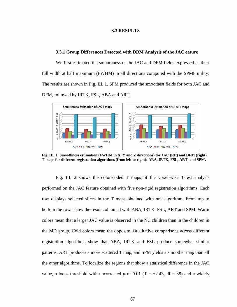
67
3.3 RESULTS
3.3.1 Group Differences Detected with DBM Analysis of the JAC eature
We first estimated the smoothness of the JAC and DFM fields expressed as their
full width at half maximum (FWHM) in all directions computed with the SPM8 utility.
The results are shown in Fig. III. 1. SPM produced the smoothest fields for both JAC and
DFM, followed by IRTK, FSL, ABA and ART.
Fig. III. 1. Smoothness estimation (FWHM in X, Y and Z directions) for JAC (left) and DFM (right)
T maps for different registration algorithms (from left to right): ABA, IRTK, FSL, ART, and SPM.
Fig. III. 2 shows the color-coded T maps of the voxel-wise T-test analysis
performed on the JAC feature obtained with five non-rigid registration algorithms. Each
row displays selected slices in the T maps obtained with one algorithm. From top to
bottom the rows show the results obtained with ABA, IRTK, FSL, ART and SPM. Warm
colors mean that a larger JAC value is observed in the NC children than in the children in
the MD group. Cold colors mean the opposite. Qualitative comparisons across different
registration algorithms show that ABA, IRTK and FSL produce somewhat similar
patterns, ART produces a more scattered T map, and SPM yields a smoother map than all
the other algorithms. To localize the regions that show a statistical difference in the JAC
value, a loose threshold with uncorrected p of 0.01 (T = ±2.43, df = 38) and a widely
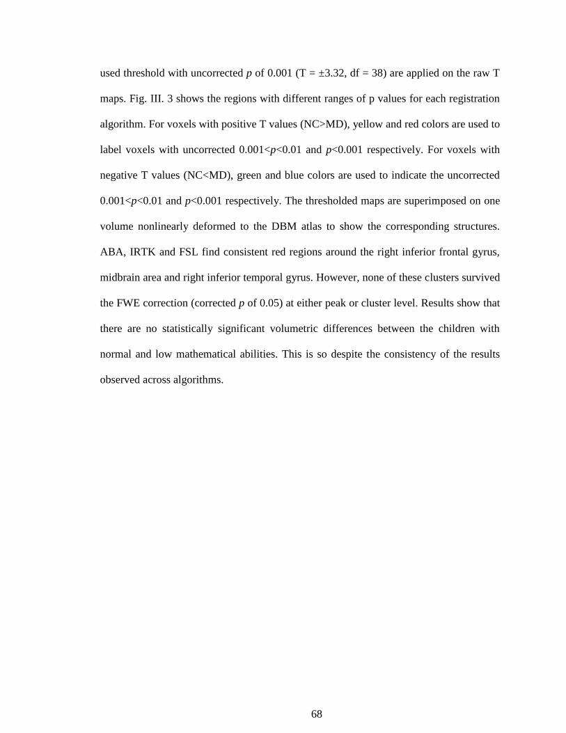
68
used threshold with uncorrected p of 0.001 (T = ±3.32, df = 38) are applied on the raw T
maps. Fig. III. 3 shows the regions with different ranges of p values for each registration
algorithm. For voxels with positive T values (NC>MD), yellow and red colors are used to
label voxels with uncorrected 0.001<p<0.01 and p<0.001 respectively. For voxels with
negative T values (NC<MD), green and blue colors are used to indicate the uncorrected
0.001<p<0.01 and p<0.001 respectively. The thresholded maps are superimposed on one
volume nonlinearly deformed to the DBM atlas to show the corresponding structures.
ABA, IRTK and FSL find consistent red regions around the right inferior frontal gyrus,
midbrain area and right inferior temporal gyrus. However, none of these clusters survived
the FWE correction (corrected p of 0.05) at either peak or cluster level. Results show that
there are no statistically significant volumetric differences between the children with
normal and low mathematical abilities. This is so despite the consistency of the results
observed across algorithms.
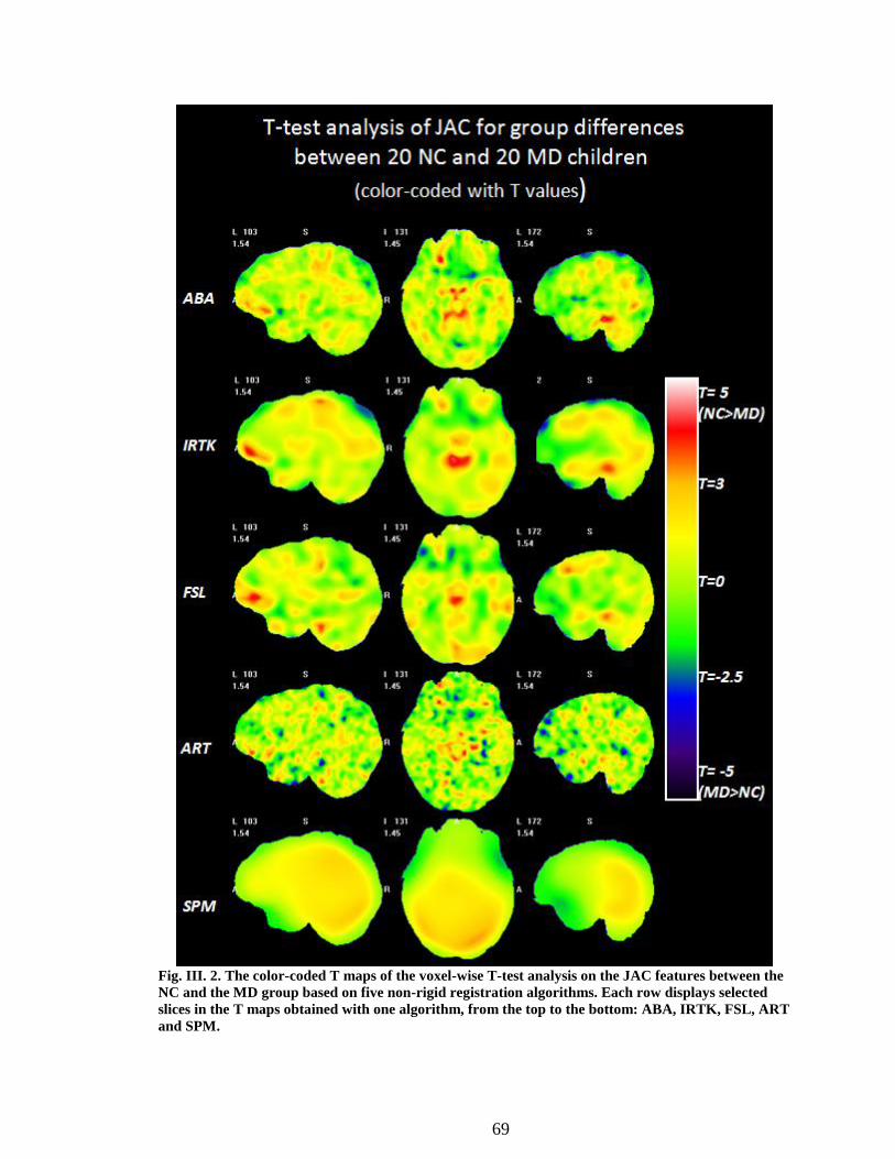
69
Fig. III. 2. The color-coded T maps of the voxel-wise T-test analysis on the JAC features between the
NC and the MD group based on five non-rigid registration algorithms. Each row displays selected
slices in the T maps obtained with one algorithm, from the top to the bottom: ABA, IRTK, FSL, ART
and SPM.

70
Fig. III. 3. The regions with different ranges of p values for DBM results for JAC based on each
registration algorithm superimposed on one volume deformed to the DBM atlas. Warm colors show
NC has larger JAC than MD, and cold colors mean the opposite. None of these clusters survived the
FWE multiple comparison correction.

71
3.3.2 Group Differences Detected with DBM Analysis of the DFM Feature
Fig. III. 4 shows the color-coded T maps of the voxel-wise T-test analysis
performed on the DFM feature between the NC and the MD group obtained with five
non-rigid registration algorithms. Warm colors mean that MD subjects have larger
anatomical variations than the NC subjects. Cold colors mean the opposite. Qualitative
comparison shows that ABA, IRTK and FSL show similar patterns, while ART and SPM
produce the least smooth and the smoothest T maps, respectively. Thresholding the T
maps with uncorrected p values of 0.01 and 0.001 leads to Fig. III. 5, showing the color-
coded regions with different ranges of the statistical significance in a similar fashion as in
Fig. III. 3. The results shown in Fig. III. 4 and Fig. III. 5 show that the MD children have
more anatomical variations than the NC children around the left temporal and occipital
lobe, the orbital-frontal area and the right insular cortex. Such differences are consistently
found across different registration algorithms although patterns vary somewhat. After
FWE correction for multiple comparisons, all the clusters that survived for the different
registration algorithms were combined to find the common regions of interests, as
explained in section 2.2.6. If at least two registration algorithms found overlapping
regions (membership threshold of 2), these were considered to be a common ROI in
which anatomical variation differences between the NC and the MD group may exist.
Fig. III. 6 displays the statistically significant clusters after the FWE corrections
for each of the five non-rigid registration methods, superimposed on one volume
nonlinearly deformed to the DBM atlas. In this figure, pixels with uncorrected p values
smaller than 0.001 (red clusters in Fig. III. 5) that are part of a statistically significant
cluster at either cluster/peak or both levels are shown in color based on their T values.

72
Each column shows the DBM results for one algorithm on the same selected views as in
Fig. III. 5.Warm colors mean that larger DFM values were observed in the MD subjects
than in the NC subjects. Cold colors mean the opposite. The line type used for the circles
reflects the statistical significance after FWE corrections for the clusters within the ROI.
If a cluster in a region is significant at both peak and cluster level, a solid circle is drawn
around the region. Dotted lines or dashed lines are drawn around a cluster that is
statistically significant at either peak level or cluster level. Three regions of interests
(ROIs) are circled with different colors: R1-Orange; R2-Red, and R3-Yellow. All five
non-rigid registration algorithms found R1 located around the left occipitotemporal
sulcus, the left fusiform gyrus (BA 37) and the cerebellum. ABA and IRTK also found
R2 around the left olfactory sulcus and the gyrus rectus (BA 47). IRTK and ART found
R3 in the right insular cortex. Table. III. 1 lists all the clusters found in each ROI by
different registration algorithms and their maximum T values, the FWE corrected p
values at peak and cluster levels, and the cluster sizes. The blue (green) colors in the table
mean the region is significant with corrected p of 0.05(0.5) based on that algorithm.
R2 and R3 each were found to be statistically significant by only two algorithms
(different pairs for each region). But Fig. III. 5 also shows that the other algorithms found
regions of difference in the same general area. For example, FSL, ART and SPM all
found yellow or red clusters around R2 that meet the loose uncorrected p threshold
(p<0.01). Also, ABA and FSL both have a relatively large red cluster (uncorrected
p<0.001) around the right insular cortex (R3). However these were not found to be
significant after FWE correction. There is also a unique cluster around the left superior

73
frontal gyrus found only by IRTK that is statistically significant at peak-level after FWE
correction (corrected p of 0.025).
Fig. III. 4. The color-coded T maps of the voxel-wise T-test analysis on the DFM features between the
NC and the MD group based on five non-rigid registration algorithms. Each row displays the
selected slices in the T maps obtained based on one algorithm, from the top to the bottom: ABA,
IRTK, FSL, ART and SPM.

74
Fig. III. 5. The regions with different ranges of p values for DBM results for DFM based on each
registration algorithm imposed on one volume deformed to the DBM atlas. Warm colors show that
NC has larger DFM than MD, and cold colors mean the opposite.
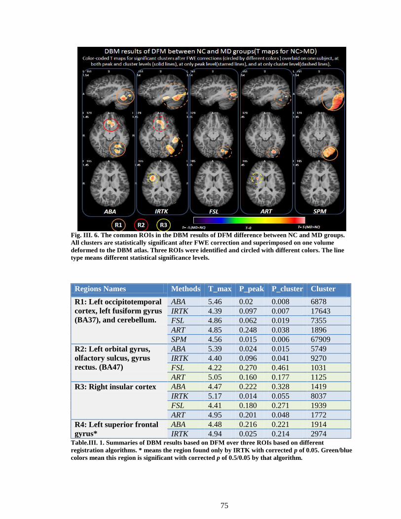
75
Fig. III. 6. The common ROIs in the DBM results of DFM difference between NC and MD groups.
All clusters are statistically significant after FWE correction and superimposed on one volume
deformed to the DBM atlas. Three ROIs were identified and circled with different colors. The line
type means different statistical significance levels.
Regions Names Methods T_max P_peak P_cluster Cluster
Size R1: Left occipitotemporal
cortex, left fusiform gyrus
(BA37), and cerebellum.
ABA 5.46 0.02 0.008 6878
IRTK 4.39 0.097 0.007 17643
FSL 4.86 0.062 0.019 7355
ART 4.85 0.248 0.038 1896
SPM 4.56 0.015 0.006 67909
R2: Left orbital gyrus,
olfactory sulcus, gyrus
rectus. (BA47)
ABA 5.39 0.024 0.015 5749
IRTK 4.40 0.096 0.041 9270
FSL 4.22 0.270 0.461 1031
ART 5.05 0.160 0.177 1125
R3: Right insular cortex ABA 4.47 0.222 0.328 1419
IRTK 5.17 0.014 0.055 8037
FSL 4.41 0.180 0.271 1939
ART 4.95 0.201 0.048 1772
R4: Left superior frontal
gyrus*
ABA 4.48 0.216 0.221 1914
IRTK 4.94 0.025 0.214 2974 Table.III. 1. Summaries of DBM results based on DFM over three ROIs based on different
registration algorithms. * means the region found only by IRTK with corrected p of 0.05. Green/blue
colors mean this region is significant with corrected p of 0.5/0.05 by that algorithm.

76
3.3.3 Group Differences Detected with DBM Analysis of the Voxel-wise
Correlation Coefficient between the DFM Feature and the WRAT-M Score.
Correlation analysis between the children’s WRAT-M scores and the anatomical
features for the entire dataset of 79 children was conducted throughout the entire brain
with the DBM technique. The results were produced with the five non-rigid registration
algorithms introduced previously. Only the DFM feature has been considered in the
correlation study, because no group volumetric differences were found between the NC
and the MD group. Fig. III. 7 shows the color-coded T maps for the voxel-wise
correlation coefficient between WRAT-M scores and the DFM feature for all 79 children.
This map was produced with an ANCOVA model, adjusted for age and gender. Each row
displays the three selected views of the T maps obtained with one algorithm. From top to
bottom, the rows show the results obtained with ABA, IRTK, FSL, ART, and SPM.
Warm colors mean negative correlation between the WART-M score and the DFM value,
while cold colors mean positive correlation. As was done in Fig. III. 3 and Fig. III. 5, a
loose threshold at uncorrected p of 0.01 (T = ±2.38, df = 74) and a regular threshold at
uncorrected p of 0.001 (T = ±3.20, df = 74) are used to threshold the T maps. Images
thresholded with these values are coded with different colors, as shown in Fig. III. 8. As
can be observed, the yellow and red clusters in Fig. III. 8 appear to be in a position that is
similar to the position of the yellow and red clusters shown in Fig. III. 5, but with smaller
cluster sizes and lower significances of uncorrected p values. None of the clusters are
statistical significant after the FWE correction.
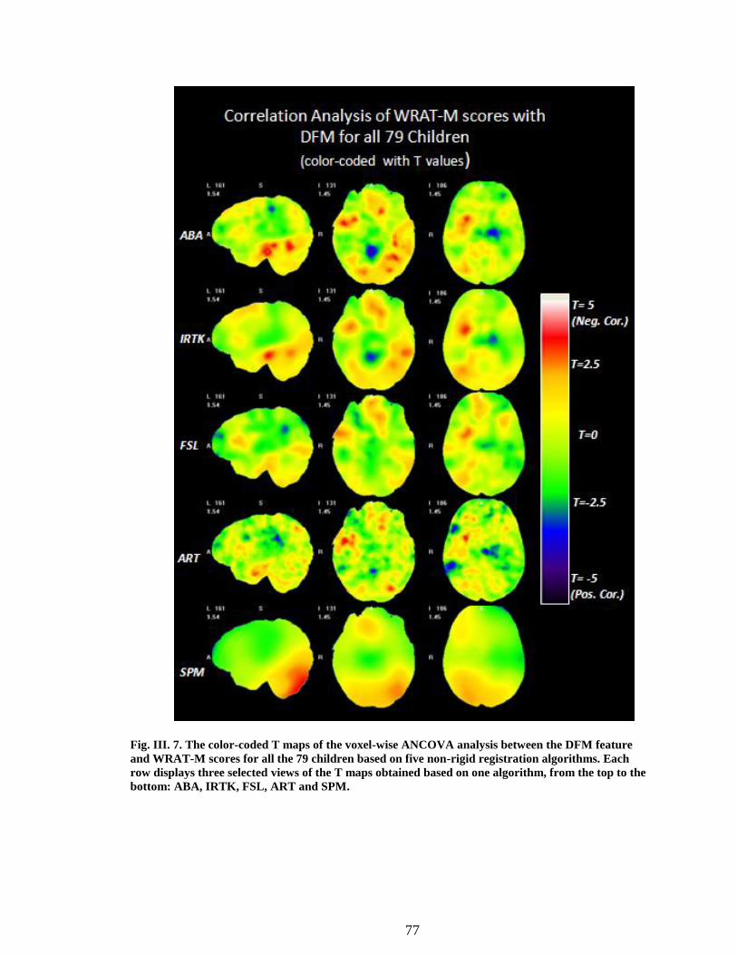
77
Fig. III. 7. The color-coded T maps of the voxel-wise ANCOVA analysis between the DFM feature
and WRAT-M scores for all the 79 children based on five non-rigid registration algorithms. Each
row displays three selected views of the T maps obtained based on one algorithm, from the top to the
bottom: ABA, IRTK, FSL, ART and SPM.

78
Fig. III. 8. The regions with different ranges of p values for DBM results of DFM correlated with
WRAT-M scores based on each registration algorithm superimposed on one volume deformed to the
DBM atlas. Warm colors show that NC has larger DFM than MD, and cold colors mean the opposite.

79
Fig. III. 9. Scatter plots for correlation analysis between the mean DFM over each ROI and the
WRAT-M scores for all the 79 children, using five different registration algorithms. Red frames
mean the correlation coefficients are statistically significant (p<0.05), blue frames mean the opposite.

80
Fig. III. 9 presents the plots showing the relation between the mean DFM over
each ROI (Y axis) and the math scores for each registration algorithm (X axis). Each
subpanel shows the regression line that has been computed, the ROI (R1, R2 or R3) to
which the plot relates (top left), the registration algorithm that has been used (bottom left),
the correlation coefficient r between the mean DFM and the WRAT-M scores (right side),
and the p value. If the correlation is statistically significant (p<0.05), the sub-panel is
marked with a red border, otherwise (p>0.05) it is drawn in blue. Because this analysis is
based on one single value/region, i.e., the mean value of the feature over the region, there
is no need for multiple comparison correction.
As can be observed, ABA, IRTK and FSL show statistically significant
correlations between the mean of the DFM over each ROI and the WRAT-M scores. This
agrees well with the color-coded clusters around R1, R2 and R3 for these algorithms in
Fig. III. 5 and Fig. III. 8. This means that the lower the child’s math score, the larger the
DFM mean values tend to be over each ROI, i.e. the more the voxels in this ROI have to
be displaced to match the atlas image with the subject’s image. FSL yielded statistically
significant correlations over R2 and R3, but not over R1. Fig. III. 8 also shows that FSL
found the correlation T maps over R2 and R3 to meet the loose uncorrected threshold of
0.01, but not over R1. SPM only finds statistically significant correlations between mean
DFM and WRAT-M scores over R1, as can be seen from Fig. III. 8. These results suggest
that there may be a correlation between brain anatomy and math performance over these
regions even though these differences are not strong enough to produce significant
regions when voxel-wise analysis and FWE correction for multiple comparisons are used.
81
3.4 DISCUSSION
Deformation-based morphometry analyses have been used to investigate brain
anatomical features for third-grade children with different mathematical performances.
The effect of five non-rigid registration algorithms (ABA, IRTK, FSL, ART and SPM)
on the DBM results have been studied when this technique is used to detect
morphological differences between two subset groups, and to explore correlations
between anatomical features and mathematical ability with the entire group of 79 third
graders. There are no statistically significant volumetric differences between the NC and
the MD groups that have been found using DBM and JAC as the feature. This leads to the
conclusion that either no differences exist or such differences are too subtle to be detected
with this data set. However, DBM analysis performed on the DFM feature found
significant anatomical variations between the two groups around three regions identified
consistently by at least two registration algorithms after FWE correction (p of 0.05). The
three regions are the left occipital-temporal cortex, left orbital-frontal cortex, and right
insular cortex. Simulated results in the next chapter indicate that FWE corrections with
corrected p of 0.05 maybe too strict. Indeed results we have produced on simulated data
sets suggest that corrected p values as high as of 0.5 preserve true positive clusters while
eliminating false positive ones. Table.III.1 lists all the p values for regions R1, R2, R3.
This table shows that with a p value of 0.25 all the algorithms find all these regions to be
statistically significant. At this p value, an additional region around the left superior
frontal gyrus is also detected by two algorithms.

82
DBM analysis on the entire 79 children did not find statistically significant
correlation between the DFM and math scores after FWE correction with the standard p <
0.05 criterion. But the p values for region R3 (around the right insular cortex) for ABA,
IRTK, FSL, and ART are 0.23, 0.27, 0.21, and 0.11, respectively. Again, with a looser
threshold of 0.25, this region would be found to be significant. Furthermore, ROI-based
correlations of mean DFM values and WRAT-M scores are statistically significant.
These findings reinforce some of the conclusions we drew in the previous chapter,
i.e., that registration algorithms indeed have an impact on DBM-based results. As we did
in the previous chapter, we would thus recommend using more than one algorithm when
conducting DBM studies. As will be shown in the next chapter, statistical analysis of the
results is also a challenge. Consensus among algorithms despite weak statistical
significance obtained with each of them may be an indication that the criteria for
inclusion are too strict and that findings are real. Our findings also expand on previous
functional studies of developmental changes in occipital-temporal cortex with age [104]
by demonstrating that a relationship between calculation skill and morphological
variability in these cortices may exist as early as third grade. The deformation field
magnitude (DFM) in the left occipitotemporal cortex and the left fusiform gyrus are
found to be statistically different between the NC and the MD group, as well as
negatively correlated with mathematical skills. Functional specialization of the left
occipitotemporal cortex has been demonstrated for various classes of visual stimuli [105,
106]. Diminished processing of written numerical symbols could explain findings of
significantly slower response times during calculation tasks in individuals with MD
compared to their same age peers [92, 93]. The left fusiform gyrus is also an area critical

83
to word/number recognition so differences in architecture in this region could be linked
to math performance.
In addition, two volumes located in the orbitofrontal cortex and the right insular
cortex showed similar behavior. These brain regions are associated with attention,
decision-making, and executive function. Functional imaging has implicated that insular
region as an important area involving emotional processing [107] and speech-motor
function [108]. In particular the right anterior insula has been identified as a key region of
interest in specific phobias [109, 110]. Morphometry study also shows a reduced insular
volume for subjects with Williams Syndrome [81] This reduction was also found by the
DBM analysis in our previous chapter. Therefore, a disruption in any one of these
cognitive processes could conceivably cause a break down in the normal course of
procedures and interrupt the processes of solving calculation problems. In view of the
evidence that young children compared to adults have increased activation in prefrontal
cortex while performing a simple calculation task [104], the increased morphological
variability in poor calculation performers may be a contributing factor to their use of less
mature strategies during problem solving and retrieval errors [92, 93]. A significant
difference between the findings in the current study and previous studies [98, 99, 101] is
that we did not find morphological differences in the parietal cortex related to
mathematical skill. The differences may be due to the behavioral task that we used, the
method of analysis, or participant characteristics such as age and severity of
mathematical disability. Although the findings from this study appear to be in accordance
with neuropsychological models and previous results, more rigorous validation,
particularly correlating with other neuroimaging modalities such as functional MRI, are

84
still warranted to confirm them. In particular, more specific descriptions of the variations
in deformation fields in terms of underlying sulcal architecture, gyral patterns or tissue
volumes should be established.

85
CHAPTER 4
AN ANALYSIS OF THE EFFECT OF NONRIGID REGISTRATION
ALGORITHMS ON DBM ANALYSIS USING SIMULATED DATASETS
4.1 INTRODUCTION
Deformation-based morphometry (DBM) analysis has been used to quantify and
characterize morphological differences between different groups, as well as to elucidate
correlations between the brain anatomy and genetic disorders or various cognitive
abilities. The DBM approach requires images from different groups to be registered
together to a brain atlas and statistically identifies morphological differences between
groups based on the deformation fields generated by a non-rigid registration algorithm.
Although several studies have compared non-rigid registration algorithms based on
segmentation performance, little work has been done to compare the effect of registration
algorithms on population differences that may be uncovered through deformation-based
morphometry.
In the previous two chapters of this dissertation, the effect of registration
algorithms on DBM analysis has been studied with five different non-rigid registration
algorithms and two very different datasets. The first dataset includes normal subjects and
patients with Williams Syndrome (WS) with large and well-documented anatomical
differences between the two groups. The other dataset contains children with a range of
mathematical abilities. In this data set, the anatomical differences, if present, are more

86
subtle than those observed in the WS dataset. Both studies have shown the DBM results
depend on the algorithm that is used. However, the lack of ground truth has limited our
ability to quantitatively compare these algorithms. The primary goal of this chapter is to
develop a framework that allows a comparison of the effects of various non-rigid
registration algorithms on DBM results with simulated ground truth. This framework
includes synthesizing realistic deformation fields and MR images, introducing various
known local deformations, performing DBM analysis with various non-rigid registration
methods, quantifying the performance of these registration methods, and studying the
effect of statistical correction methods on the results. A software pipeline integrating the
different blocks that form this framework has been developed to produce data sets on the
Advanced Computing Center for Research and Education (ACCRE) cluster to take full
advantage of available parallel computational resources.
In this study, we have used the statistical simulation of deformations (SSD)
method proposed by Xue et al. to simulate realistic deformation fields and MR images
[111]. In the training phase of the SSD model, a wavelet-based principal component
analysis algorithm (W-PCA) decomposes a set of training deformation fields using the
Wavelet-Packet Transform (WPT) and subsequently captures within-scale statistics via
hierarchically organized PCA models [112]. In the simulation phase, realistic
deformation fields are produced by drawing sample parameter values from the
parameters’ probability density functions (pdfs). The fields produced with this approach
are then adjusted to constrain the value of the Jacobian determinant and regularized with
a nested Markov Random Field (more details can be found in [111] and the software that
implements this technique can be found at www.rad.upenn.edu/sbia/software.) The
87
deformation fields produced by this algorithm can then be used to generate a series of
images. Several parameters can be adjusted to manipulate the SSD model to control the
desired amount of inter-subject anatomical variation. The adjustment of parameters
allows the creation of populations with a controllable amount of variability. For instance,
we can produce populations in which differences are detected before multiple comparison
correction but not after correction.
After a series of images was created with the aforementioned technique, an
assortment of local deformations was introduced to simulate pathologies and differences
between populations. These local deformations were simulated with local radial
symmetric deformation fields used to deform the simulated MRI. These were also used
to define ground truths when comparing DBM results obtained with various registration
algorithms. As was the case in the previous chapters, the five nonrigid registration
algorithms used in this study are: (1) The Adaptive Bases Algorithm (ABA) [26], (2) The
Image Registration Toolkit (IRTK) [27], (3) The FSL Nonlinear Image Registration Tool
(FSL) [64], (4) The Automatic Registration Tools (ART) [28], and (5) The normalization
algorithm in SPM8 (SPM) [29]. For each registration algorithm, DBM analysis was
performed between various simulated groups (further details on these various groups are
provided below). The same statistical analysis that was performed on the real data sets
was applied (see section 1.1.2). DBM results obtained with the five non-rigid registration
algorithms were then compared to the known ground truth both qualitatively and
quantitatively.
The remainder of this chapter is organized as follows. First, we describe in some
details the framework that has been developed to generate the data sets, including
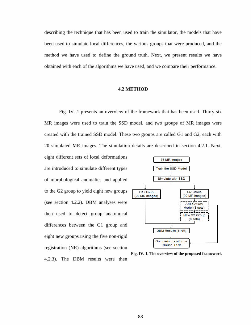
88
describing the technique that has been used to train the simulator, the models that have
been used to simulate local differences, the various groups that were produced, and the
method we have used to define the ground truth. Next, we present results we have
obtained with each of the algorithms we have used, and we compare their performance.
4.2 METHOD
Fig. IV. 1 presents an overview of the framework that has been used. Thirty-six
MR images were used to train the SSD model, and two groups of MR images were
created with the trained SSD model. These two groups are called G1 and G2, each with
20 simulated MR images. The simulation details are described in section 4.2.1. Next,
eight different sets of local deformations
are introduced to simulate different types
of morphological anomalies and applied
to the G2 group to yield eight new groups
(see section 4.2.2). DBM analyses were
then used to detect group anatomical
differences between the G1 group and
eight new groups using the five non-rigid
registration (NR) algorithms (see section
4.2.3). The DBM results were then
Fig. IV. 1. The overview of the proposed framework

89
compared both quantitatively and qualitatively with the ground truth defined with a
criterion derived from the Jacobian of the local deformations, as explained in section
4.2.2.
4.2.1 Simulation with the SSD Model
Thirty-six MR brain images obtained from normal children (20 males and 16
females, 8.9±0.4 years old) were used in this section. Each image was corrected for
intensity inhomogeneity with the N3 algorithm and rigidly aligned to the MNI template
to correct for differences in pose and orientation during acquisition (see section 1.3.1 for
details). Atlas-based segmentation combined with the FSL Brain Extraction Tool [113]
was used to strip the skulls for all the 36 MR images. One subject was selected as the
atlas, to which all the other 35 subjects were registered with affine transformations. The
affinely transformed images were then non-rigidly registered to the atlas to produce
deformation fields to train the SSD model.
Fig. IV. 2. The various steps used to train the SSD models and to produce test images.

90
Fig. IV. 2 illustrates the steps used to train the model and produce images. To
reduce possible bias of the SSD model towards one particular registration algorithm, the
thirty-five subjects in the training dataset were randomly assigned into five groups of
seven subjects. For each group, one non-rigid registration algorithm was used to register
the seven images to the atlas image. For each group, this registration produced seven
deformation fields (the colored arrows in the figure shows that training deformation fields
were produced by different algorithms). Each registration algorithm outputs deformation
fields in a different format. These are then converted to the format required for the
training of the SSD model. The 35 format-adjusted deformation fields were used to train
the SSD model, yielding a series of PCA and wavelet parameters. Because deformation
fields produced by the five algorithms were used in the training, simulated deformation
fields should not have characteristics that favor one algorithm over the other.
After the creation of the SSD model, the distribution of the parameters was
sampled to produce a set of 40 simulated deformation fields. By applying the inverse of
these deformation fields to the atlas, 40 simulated realistic MR images were created and
randomly assigned into 2 groups, called the G1 and the G2 group. The anatomical
differences between the G1 and the G2 groups detected with the five non-rigid
registration algorithms were subsequently analyzed with DBM analysis. The inter-subject
anatomical variation in the simulated images can be adjusted by limiting the range of
parameter values and this range was iteratively adjusted based on the DBM results to
ensure that no statistically significant anatomical differences between the G1 and G2
groups exist.

91
4.2.2 Simulation with the Growth Models
Local displacements were simulated to introduce various pathologies in the G2
group and to derive the ground truth for subsequent comparisons of DBM results
obtained with different non-rigid registration algorithms. Eight sets of local displacement
models were produced in total based on two base growth models (GM1 and GM2), each
comprising several local growths patterns with different characteristics.
Each local growth is a radially symmetric deformation field. The displacements
along the x, y, and z directions are obtained by coordinate conversions from the
deformation field magnitude using the trigonometric functions. The deformation field
magnitude (DFM) is a function of the Euclidean distance ( )from each voxel
to the seed location as described in the equations (4.1-4.3) below:
( ) √( ) ( )
( ) , (4.1)
( ) { ( ) ( )
( ) ( ) ( ) , (4.2)
( ) ( )
( ) ( )
( ) ( )
,(4.3)
where R is the growth radius, α is the increase rate inside the radius, and β is the
decreased rate outside the radius. Growth models are combined with the deformation
fields to produce local deformations spread over the brain that simulate small and large
differences between image volumes.
Fig. IV. 3. Coordinates conversion.

92
Fig. IV. 4. The illustration of GM1 and GM2.
Fig. IV. 4 shows the local deformations used in the two base groups: GM1 (top
panel) and GM2 (bottom panel). The left column shows the parameter values used for
each local growth, the middle column shows the color-coded DFM where it is larger than
1 mm overlaid on the atlas, the third column shows a deformed grid that permits the
visualization of the local deformation field in the GM1 and GM2 models (for comparison,
the average displacements between the template and the various volumes produced by the
SSD simulator in these regions is on the order of 3 mm). The rightmost column shows the
region over which the magnitude of the DFM is larger than one millimeter. These DFM
masks were used to characterize the displacement radius of the local growth, shown in
the left panel in Fig. IV. 5. In this figure, the blue and red bars represents the local growth
in the GM1 and GM2 groups respectively. To simulate more variation in local differences,
the seed location for each growth model is randomly perturbed along each direction by
20%, 50%, and 80% of their corresponding displacement radius. For each percentage
value, 20 samples drawn from a uniform distribution were used to displace the seed

93
locations in GM1 and GM2, yielding 20 new image volumes. Eight sets of local
deformations derived from the GM1 or GM2 base models with different displacements
were produced and combined with the deformation fields used to generate the 20 images
in the G2 group.
Fig. IV. 5. The displacement radius and growth radius for local growths in GM1 and GM2.
Because we create differences between populations by introducing local
expansion, in this chapter, we limit our study to the JAC feature. To define a ground truth
to which we compare the DBM results based on various algorithms, we compute the JAC
of the simulated fields and threshold these to 1.1. The growth sizes based on this criterion
for each local growth in the GM1 (in blue) and GM2 (in red) are shown in the right panel
of Fig. IV. 5. Fig. IV. 6 shows the final ground truth for each set of growth model. This
ground truth has been defined as the union of the 20 masks in which the JAC is larger
than 1.1.

94
Fig. IV. 6. The ground truth for each set of the growth model.
4.2.3 Deformation-based Morphometry (DBM) Analysis
Fig. IV. 7 shows the flowchart of the various steps used for the DBM analysis of
the simulated datasets. Starting from the atlas (top left), the G1group (shown with red
frames) and the G2 group (shown with blue frames) were first simulated with the SSD
model. This produced two groups of simulated images with 20 volumes in each group.
The two local growth models (GM1 and GM2) combined with different seed
displacements (DS0-DS3) were applied to each subject in the G2 group, yielding 8
groups of MR images. The deformed grids for each growth model are shown in this
flowchart, GM1 has five big local growths and GM2 has ten smaller local growths. Each
group is named after the GM choice and the displacement percentages, i.e.
G2_GM2_DS2 means the G2 group deformed by GM2 with a random displacement of
the seeds location by 50%. The other group names can be interpreted in the same way.
There are twenty images in each group which each have been deformed by one radially
symmetric local growth with a possible displacement of the seed. The ground truth

95
computed for each group is shown in Fig. IV. 6. In the remainder of this chapter,
G2_GM*_DS* represents any of the 8 deformed groups.
Fig. IV. 7.The flowchart for DBM analysis on simulated datasets.
DBM analyses were performed between the G2_GM*_DS* group and the G1
group using the five non-rigid registration algorithms: ABA, IRTK, FSL, ART, and SPM.
The JAC features were calculated to characterize volumetric differences between groups.
Voxel wise t-tests were performed between the JAC values for each of the 8 groups and
the G1 group, yielding 8 different T maps for each registration algorithm (each algorithm
is shown in a different color). At the bottom right of Fig. IV. 7, T maps obtained with

96
each registration method are compared with the ground truth obtained from the growth
models.
4.2.4 Quantitative Comparisons
Quantitative comparisons of registration algorithms were based on comparing
differences detected with DBM analysis to the ground truths. As was done for the
analysis of subject data sets, T maps were first created. These are then thresholded at an
uncorrected p value of 0.001 (T=3.312, df=38). This thresholding yields a series of
clusters for each algorithm. Then a Family Wise Error (FWE) corrected p of 0.05 at
either the cluster level or peak level was used to correct for the multiple comparison
issues (some clusters that survive the uncorrected p of 0.001 may not be statistically
significant after the FWE correction). The metric used to quantify the performance of the
registration algorithms is the cluster detection rate (CDR). The CDR values were
computed both before and after FWE corrections to study the effect of FWE correction
on DBM results for each algorithm. For this metric, the True Positive (TP), False
Negative (FN), and False Positive (FP)
concepts illustrated in Fig. IV. 8 have been
used. In this figure, the light red circle
represents the ground truth, and the blue
circle denotes the results produced by each
registration algorithm. The definition of TP,
FN and FP for this metric is based on the
cluster count. Fig. IV. 8. FN, TP, FP.

97
The cluster detection rate (CDR) is defined as the number of TP clusters divided
by the number of clusters in the ground truth plus the number of FP clusters:
The total number of clusters in the ground truth is five for the large growth model
(four in the GM1_DS3 because two clusters were merged due to seed displacements) and
ten for the small growth model. For each of the clusters in the ground truth, we have used
the heuristic rule that if any voxel in that cluster is detected to be statistically significant
by one registration algorithm, that cluster is labeled as a TP for that algorithm. The final
TP for this algorithm will range from 0 to the total number of clusters in the ground truth.
When one cluster in the ground truth is detected as multiple smaller clusters by one
algorithm, only one TP is counted. The number of artificially broken (AB) clusters into
which a cluster is broken is also recorded. If one registration algorithm finds a cluster that
does not correspond to a ground truth region, this cluster is counted as a FP. The CDR is
also called Jaccard similarity or Tanimoto coefficient [114]. The CDR is zero if none of
the clusters in the ground truth have been detected by DBM. When DBM detects all the
clusters in the ground truth and there is no FP, the CDR is 1. The higher the CDR, the
better that registration algorithm can detect known group anatomical differences with
DBM analysis.

98
4.3 RESULTS
4.3.1 Simulated Images with the SSD Model
Fig. IV. 9 shows four examples of simulated MR images in the G1 group (top
panel) and in the G2 group (bottom panel). The atlas image is shown on the left.
Fig. IV. 9. Examples of simulated images with the SSD model in G1 (top) and G2 (bottom) groups.
As can be seen, the simulated MR images look very realistic while showing
anatomical differences. Fig. IV. 10 displays the T maps for the JAC features between the
G1 and the G2 group based on five non-rigid registration algorithms (left to right): ABA,
IRTK, FSL, ART, and SPM. Warm colors indicate the features values are larger for the
G2 images than the G1 images; cold colors mean the opposite. The red square box around
the T map means that no cluster survived the uncorrected p of 0.001. The white square
box means that no cluster survived the FWE corrected p of 0.05, though some clusters
may have survived the uncorrected p of 0.001, the number of such clusters is listed at the
bottom right within each box.
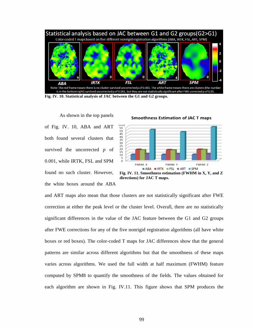
99
Fig. IV. 10. Statistical analysis of JAC between the G1 and G2 groups.
As shown in the top panels
of Fig. IV. 10, ABA and ART
both found several clusters that
survived the uncorrected p of
0.001, while IRTK, FSL and SPM
found no such cluster. However,
the white boxes around the ABA
and ART maps also mean that those clusters are not statistically significant after FWE
correction at either the peak level or the cluster level. Overall, there are no statistically
significant differences in the value of the JAC feature between the G1 and G2 groups
after FWE corrections for any of the five nonrigid registration algorithms (all have white
boxes or red boxes). The color-coded T maps for JAC differences show that the general
patterns are similar across different algorithms but that the smoothness of these maps
varies across algorithms. We used the full width at half maximum (FWHM) feature
computed by SPM8 to quantify the smoothness of the fields. The values obtained for
each algorithm are shown in Fig. IV.11. This figure shows that SPM produces the
Fig. IV. 11. Smoothness estimation (FWHM in X, Y, and Z
directions) for JAC T maps.

100
smoothest field, followed by IRTK, FSL, ART, and ABA. In previous chapters, the
smoothness of the JAC fields for these registration algorithms have also been calculated
(see Fig. II. 7 and Fig. III. 1). SPM consistently produces the smoothest fields. The main
difference is that ABA produces the least smooth field in the simulated data, while ART
produces the least smooth field in both real datasets.
4.3.2 Simulated Images with the Growth Models
Fig. IV. 12 presents an axial view of a simulated image in the G2_GM0_DS0
(left most), the G2_GM1_DS0 (0% displacement), the G2_GM1_DS1 (20%
displacement), the G2_GM1_DS2 (50% displacement), and the G2_GM1_DS3 (80%
displacement) groups. The middle row shows zoomed in regions of these images, with
the red arrows pointing to visual differences with the left most image. The green dots
show the original seed location for the local growth models. In the GM1 images, there is
a relatively large local growth located in the white matter region. The figure shows the
effect of displacing the seed has on the generated images. The color-coded images are
difference images computed between the deformed images and the reference one. The
rightmost color-coded image shows the effect of a large seed displacement. Fig. IV. 13
shows the same thing for images in the GM2 group. The differences are less obvious as
the growth size in the GM2 group is small, which also leads to smaller displacements.

101
Fig. IV. 12. An example of simulated images in the G2 group and four GM1 based groups. The
zoomed views are shown in the middle panel, and bottom panel shows the intensity differences. The
red arrows point to the visual differences with the left most image.
Fig. IV. 13. An example of simulated images in the G2 group and four GM2 based groups. The
zoomed views are shown in the middle panel, and bottom panel shows the intensity differences.

102
4.3.3 Qualitative Comparisons of Registration Algorithms
Fig. IV. 14 presents a series of images that permit the qualitative comparison of
DBM results obtained for the JAC feature with the various non-rigid registration
algorithms. Each row corresponds to one deformation model; the first four to the GM1
(large growth) model and the last four to the GM2 model (small growth). Within each
category the 4 rows correspond to the various amount of offset that has been applied to
the seeds, i.e., DS0-0%, DS1-20%, DS2-50%, and DS3-80%. In each case, the ground
truth (i.e., the union of the regions over which JAC is larger than 1.1) is listed in the left
most column. The second column from the left shows the region over which the
magnitude of the deformation field is larger than 1 mm to give the reader a sense of the
size of the displacement range. The following columns show results obtained with ABA,
IRTK, FSL and ART. The color coded maps are the T maps thresholded at an
uncorrected p of 0.001 (T=3.319, df=38). SPM did not find any cluster that survived this
test in any of the groups so these results are not shown. Warm colors mean that a larger
feature value was observed in the deformed groups than in the G1 group. Clusters that are
not statistically significant after FWE corrections (corrected p<0.05) at either cluster or
peak level are marked with white circles.
A number of observations can be made from these results. Focusing on the large
growth model in Fig. IV. 14, differences between populations become more difficult to
detect as one move from the 0% model to the 80% model because these differences are
more diffuse and the variability introduced by the growth model becomes more difficult
to separate from the anatomical variability introduced by the SSD model. This is reflected
in the results. All four algorithms were able to detect all five clusters in the 0% and 20%

103
cases and these were deemed significant after FWE correction. The extent of these
clusters is approximately the same for all the algorithms. In the 50% seed displacement
case, all four algorithms detected all the clusters but most of them were eliminated after
FWE correction. At 80% most of the clusters are missed (only FSL finds one that is
statistically significant).
For the small growth model, ABA and ART detect the majority of the clusters at 0%
displacement while IRTK and FSL missed most of them. The substantial difference
observed between ABA and ART on the one hand and IRTK and FSL on the other can be
attributed to the smoothness of the deformation fields produced by these algorithms. The
smallest growth areas are below the detection threshold of these two algorithms. The data
is a little bit more difficult to interpret for ABA and ART. At 0% seed offset both ABA
and ART detect seven out of the ten regions of difference but they do not eliminate the
smaller ones and keep the larger ones. Whether or not a region is kept also depends on
the parameters that have been used in the growth model and on the location of the seed.
On the left side of the head, the growth parameters are such that displacements within the
growth region are larger than displacements in the growth regions on the right side of the
head. This leads to larger Jacobian values within these regions, to larger T values, and
subsequently to the labeling of the regions as being statistically significant. In the 50%
seed displacement case, most of the survived clusters have seeds located intensity
homogeneous regions, e.g. white matter or thalamus.

104
Fig. IV. 14. Qualitative comparison of registration algorithms on DBM results of JAC with the
ground truth for 8 different sets of growth models (thresholded at uncorrected p of 0.001). White
circles mean that the cluster is not statistically significant after FWE corrected p of 0.05.

105
4.3.4 Quantitative Comparisons of Registration Algorithms
Table. IV. 1 and Fig. IV. 15-16 present a more quantitative comparison between
algorithms based on the cluster detection rate (CDR) parameters introduced before. Table.
IV. 1 presents all the information needed to calculate the CDR values for each algorithm
and each growth model before and after FWE correction. In this figure, TP, FP, and CDR
refer to True Positive (green cells in the table), False Positive (pink cells in the table), and
cluster detection rate (gray cells in the table), respectively. BF denotes before FWE
correction and AF denotes after FWE correction with corrected p of 0.05.
Table. IV. 1. Summaries of DBM results of JAC based on different registration algorithms
comparing to ground truth, in terms of TP, FP and CDR, for eight GM1 and GM2 derived groups.
Growth Model GM1 GM2
Displacements DS0 DS1 DS2 DS3 DS0 DS1 DS2 DS3
Truth 5 5 5 4 10 10 10 10
TP
BF
ABA 5 5 5 2 10 10 8 5
IRTK 5 5 5 2 2 2 2 1
FSL 5 5 5 2 4 3 3 2
ART 5 5 5 2 9 9 8 6
AF
ABA 5 5 1 0 7 7 2 0
IRTK 5 5 2 0 0 0 0 0
FSL 5 5 2 1 1 1 1 0
ART 5 5 2 0 7 7 4 0
FP
BF
ABA 10 9 10 12 9 11 12 8
IRTK 0 0 0 0 1 1 1 0
FSL 0 0 0 0 0 0 0 0
ART 3 4 3 2 7 8 6 7
AF
ABA 0 0 0 0 0 0 0 0
IRTK 0 0 0 0 0 0 0 0
FSL 0 0 0 0 0 0 0 0
ART 0 0 0 0 0 0 0 0
CDR
BF
ABA 0.33 0.36 0.33 0.13 0.53 0.48 0.36 0.28
IRTK 1.00 1.00 1.00 0.50 0.18 0.18 0.18 0.10
FSL 1.00 1.00 1.00 0.50 0.40 0.30 0.30 0.20
ART 0.63 0.56 0.63 0.33 0.53 0.50 0.50 0.35
AF
ABA 1.00 1.00 0.20 0.00 0.70 0.70 0.20 0.00
IRTK 1.00 1.00 0.40 0.00 0.00 0.00 0.00 0.00
FSL 1.00 1.00 0.40 0.25 0.10 0.10 0.10 0.00
ART 1.00 1.00 0.40 0.00 0.70 0.70 0.40 0.00

106
Fig. IV. 15 presents the CDR results graphically. This figure shows that at a p
value of 0.05, FWE correction is efficient in eliminating false clusters but also that, in
many instances, it leads to the elimination of true positive clusters. FWE correction
improves the CDR for ART and ABA for the large deformation model with 0% and 20%
seed perturbation. It does, however, degrade the CDR for every algorithm for the large
growth model with 50% and 80% seed perturbation. For the small deformation model,
FWE improves the CDR for ABA and ART with 0% and 20% seed perturbation when it
degrades the performance of IRTK and FSL for these same cases. It degrades the
performance of all the algorithms for seed offsets of 50% and 80%. In general, with the
data sets used in this study, FWE tends to be too conservative and leads to the elimination
of TP clusters. Fig. IV. 16 presents CDR results when the p value after FWE correction is
increased to 0.1 and 0.5. These results indicate that, with our data set, a much less
conservative threshold of 0.5 can be used without increasing the number of false positives.
Fig. IV. 15. Cluster Detection Rate (CDR) for DBM using JAC before and after FWE corrections
(corrected p of 0.05) for GM1 and GM2 derived groups.

107
Fig. IV. 16. Cluster Detection Rate (CDR) for DBM using JAC when using FWE corrected p of 0.1
and 0.5 for GM1 and GM2 derived groups
4.4 DISCUSSION
This chapter has presented a computational pipeline that permits the creation of
simulated data sets with known differences. The pipeline has been used to study the
performance of several non-rigid registration algorithms when trying to detect small and
large local differences between populations. Qualitative and quantitative comparisons of
these registration algorithms have shown that a clear characterization of algorithms
performance is a challenging task and that the statistical analysis of the results is also
difficult. Detectability of regions of difference depends not only on the smoothness of the
deformation field that is produced by the algorithms but also on the nature and position of
the growth regions. As would be expected, with smoother fields it is more difficult to
identify small localized differences between populations. Our results indicate that, in
general, algorithms that are capable of localizing these small localized differences also
are capable of localizing larger regions. In chapters 2 and 3, we have suggested that

108
agreement between algorithms could be an indication of true differences between
populations despite a lack of statistical significance found by any of these algorithms.
Our simulations support this statement. Looking at the small displacement results, two
algorithms, i.e., ABA and ART are capable of detecting the smallest clusters. As shown
in Table. IV. 1, ABA detects 10, 10, 8, and 5 TP clusters in the DS0, DS1, DS2, and DS3
data sets of GM2, respectively. These numbers are 9, 9, 8, and 6 for ART. ABA detects 9,
11, 12, and 8 FP clusters while ART detects 7, 8, 6, and 7 FP clusters. Taking the
intersection of all these regions without any correction for multiple comparison produces
9, 9, 8, 4 TP and 0, 0, 0, 0 FP. Combining these leads to a CDRs equal to 0.9, 0.9, 0.8,
and 0.4 for the GM2 DS0, DS1, DS2, and DS3 data sets. These are better CDRs than
those obtained with FWE correction. This is due to the fact that FP occurs at different
locations with ABA and ART but that TP areas are stable across algorithms. The same
thing can be done for the large displacement models. Here, a number of combinations
could be used because all four algorithms behave similarly. Considering again ABA and
ART, Table.IV.1 shows that ABA detects 5, 5, 5, and 2 TP clusters in the DS0, DS1, DS2,
and DS3 data sets of GM1, respectively. These numbers are 5, 5, 5, and 2 for ART. ABA
detects 10, 9, 10, and 12 FP clusters when ART detects 3, 4, 3, and 2 FP clusters. Taking
the intersection of these two sets leads to 5, 5, 5, 1 TP and 0, 0, 0, 0 FPs. Combining
these leads to CDRs that are 1, 1, 1, and 0.25 for the GM1 DS0, DS1, DS2, and DS3 data
sets. These are equal to the CDRs obtained after FWE for any of the algorithm for the
DS0 and DS1 groups, substantially better than the CDR after FWE correction for all the
algorithms for the DS2 group and better than the CDR for all the algorithms expect FSL
for the DS3 group.

109
CHAPTER V
SUMMARY AND FUTURE WORK
The overall goal of this dissertation was to assess the effect of registration
algorithms on DBM-based findings. DBM is routinely used to detect differences between
populations but studies are usually conducted with only one registration algorithm with
which the research group is most familiar. In fact, we do not know of any other study that
has thoroughly investigated this question. Multiple comparisons issues related to DBM
analysis are known and methods have been proposed to address these, but whether or not
these techniques are efficient is also not well documented. After the extensive
comparison of five well known registration algorithms, the main conclusions that can be
drawn from this work are that (1) DBM-based findings are indeed dependent on the
registration algorithm that is used and (2) the FWE multiple-correction scheme that is
commonly used may be over-conservative.
Dependence of DBM findings on the registration algorithms can lead to very
different conclusions when comparing populations. In chapter 2, we have shown that the
volumetric differences between normal control (NC) subjects and subjects with Williams
Syndrome (WS) may occur around the bilateral insular cortex and putamen, as well as the
cerebellum, based on DBM results found by ABA, IRTK, FSL, and ART. However, the
DBM results based on SPM normalization are qualitatively and quantitatively different,
i.e. this technique finds only one unique large cluster located in the superior frontal cortex.
There are also a number of statistically significant clusters found by only one or two

110
registration algorithms. For example, ABA found a unique cluster around the anterior
cingulated cortex, while FSL and ART both found a cluster around the splenium of the
corpus callosum. For the anatomical variation differences between the NC and WS group,
two consistent regions located bilaterally around the orbitofrontal cortex were found by
all the registration algorithms except SPM. Nevertheless, FSL found two other unique
clusters around the left inferior and superior fontal gyrus. In chapter 3, DBM analyses
using the DFM features have discovered statistically significant anatomical variations
between normal children and children with mathematical difficulties. To the best of our
knowledge, this is the first report that brain anatomy may correlate with the level of
mathematical performance in a relatively large population of third graders.
All five non-rigid registration algorithms found clusters around the left occipital-
temporal cortex and the fusiform gyrus, though these clusters vary in size and shape
across algorithms (see Fig. III. 6). But, ABA and IRTK also found one region around the
left orbital-frontal cortex; IRTK and ART each detected another cluster in the right
insular cortex. Moreover, IRTK produced a unique cluster at the left superior frontal
gyrus, which was not found by any other algorithms. The discrepancy between results
obtained with various registration algorithms is possibly rooted in their registration
mechanisms, e.g. the similarity measure and the modeling of the deformation fields. In
general, larger clusters are usually generated by the algorithm that yields smoother
deformation fields, and vice versa. Our results also show that DBM results need to be
interpreted with care and that the characteristics of the registration algorithm that is used
need to be taken into consideration in the interpretation process.

111
Because the lack of ground truths makes it difficult to compare algorithms under
controlled conditions, we embarked on an effort to produce simulated data sets in which
known differences between populations could be introduced. These data sets not only
confirmed what had been observed with the real data, i.e., different algorithms lead to
different results, but also that correction for multiple comparisons does not perform
equally well for every algorithm. The smoothness of the field is used when performing
FWE correction. Our results indicate that FWE correction tends to perform better for
algorithms that produce less smooth fields (ABA and ART) than for those that produce
smoother fields (IRTK and FSL). For instance, FWE correction improves the CDR for
ABA and ART for both deformation models with 0% and 20% seed perturbation, because
the false positive cluster produced by ABA and ART are all eliminated by FWE
correction. But the CDR for IRTK and FSL stay the same before and after FWE
correction for big growth model, because the two algorithms have no false positive
clusters. Nevertheless, the FWE correction degrades the CDR performance for all
algorithms in both growth models with 50% and 80% seed offset and for IRTK and FSL
in small growth models with 0% and 20% seed offset, which is all due to the fact that
many true positive clusters are eliminated after FWE correction (see Table.IV.1). Overall
this correction technique appears to be over-conservative using corrected p threshold of
0.05 based on this dataset.
Based on our work, we believe there is value in using more than one algorithm
when performing DBM analysis. The open question is to determine how to interpret the
results produced by these algorithms. Should statistically significant regions produced by
any algorithm be considered to be significant, should consensus between algorithms be

112
used to increase confidence in the findings, etc.? For instance, in chapter 3 we have found
a consistent focal region (region R3 in Fig. III. 6) in the general area of the right insular
cortex. This region was deemed to be significant by two algorithms (IRTK and ART) but
not by ABA (p = 0.22) and FSL (p = 0.18). In the correlation study of DFM with the
WRAT-M scores for all the 79 children, this region is found to be statistically significant
by all registration algorithms except SPM when an uncorrected p-value threshold of
p<0.001 is used. Despite the fact that FWE correction performed on the correlation
feature does not produce any significant clusters at the customarily used corrected p <
0.05 threshold (corrected p: ABA-0.23, IRTK-0.27, FSL-0.21, ART=0.12), the
consistency of the findings by all four algorithms suggests the existence of a relation
between anatomy and math ability in this region. As our simulation results have shown,
a simple scheme in which regions of difference found by several algorithms are kept and
those that are found by only one are eliminated leads to better results than standard FWE
correction.
The simulation framework we have developed has already been useful in
analyzing and comparing registration algorithms but it is only a beginning and it could be
expanded in a number of directions. First of all, we only use a single reference volume,
which we deform with the deformation fields we produce. More variability in the data
sets could be introduced by using more than one reference volume. More sophisticated
techniques could also be used to introduce differences between populations. For instance,
Karacali et al. [115] have proposed a method that permits simulating local growth or
atrophy with a topology-preserving transformation model that generates a deformation
field with a desired level of trophy or growth by minimizing the difference between its

113
Jacobian determinants and the desired one. Such desired Jacobian patterns can thus serve
as the ground truth in the comparison stage.
This framework could also be used to evaluate the advantages and disadvantages
of various methods aiming at combining results produced by several registration
algorithms. As mentioned earlier, using multiple registration algorithms could be
beneficial when performing DBM analysis but the best way to do it needs to be
investigated. Recently, Koikkalainen et al. [116] has shown that multi-template tensor-
based morphometry yields statistically significantly better classification results than the
single-template method. Multi-registration and multi-scale deformation based
morphometry (MM-DBM) thus appear to be an interesting direction for future work as
group anatomical differences could occur at different scales. These differences can be
uncovered by varying the smoothness of the fields. The information from multiple
registration algorithms or from a single algorithm with different smoothing kernels could
be combined at different stages of DBM analysis, e.g.: 1) average the deformation fields,
2) average the JAC or DFM maps, 3) average the T maps, or 4) define voting schemes as
the one we have used in our simulation study.
The thesis examined by this dissertation is that the choice of registration
algorithm has a significant effect on DBM. In this work, we have compared the outputs
of various algorithms to verify that thesis. In order to facilitate spatial comparisons, we
have applied each algorithm to a single atlas constructed by only one of these algorithms
instead of employing algorithm-specific atlases. This choice may have reduced the
variation across algorithms, but even with this reduction, the thesis is confirmed:
Changing the registration algorithms has a significant effect on DBM.

114
REFERENCES
[1] J. G. Csernansky, S. Joshi, L. Wang, J. W. Haller, M. Gado, J. P. Miller, U.
Grenander, and M. I. Miller, "Hippocampal morphometry in schizophrenia by
high dimensional brain mapping," Proc Natl Acad Sci U S A, vol. 95, pp. 11406-
11, Sep 15 1998.
[2] D. Mamah, L. Wang, J. G. Csernansky, J. P. Rice, M. Smith, and D. M. Barch,
"Morphometry of the hippocampus and amygdala in bipolar disorder and
schizophrenia," Bipolar Disord, vol. 12, pp. 341-3, May.
[3] C. Davatzikos, M. Vaillant, S. M. Resnick, J. L. Prince, S. Letovsky, and R. N.
Bryan, "A computerized approach for morphological analysis of the corpus
callosum," J Comput Assist Tomogr, vol. 20, pp. 88-97, Jan-Feb 1996.
[4] M. F. Casanova, R. D. Sanders, T. E. Goldberg, L. B. Bigelow, G. Christison, E.
F. Torrey, and D. R. Weinberger, "Morphometry of the corpus callosum in
monozygotic twins discordant for schizophrenia: a magnetic resonance imaging
study," J Neurol Neurosurg Psychiatry, vol. 53, pp. 416-21, May 1990.
[5] F. L. Bookstein, P. D. Sampson, A. P. Streissguth, and P. D. Connor, "Geometric
morphometrics of corpus callosum and subcortical structures in the fetal-alcohol-
affected brain," Teratology, vol. 64, pp. 4-32, Jul 2001.
[6] J. Ashburner, K. Friston, and W. Penny, Chapter 6: Morphometry. Human Brain
Function, Second Edition, 2004.
[7] J. Ashburner, C. Hutton, R. Frackowiak, I. Johnsrude, C. Price, and K. Friston,
"Identifying global anatomical differences: deformation-based morphometry,"
Hum Brain Mapp, vol. 6, pp. 348-57, 1998.
[8] C. Gaser, H. P. Volz, S. Kiebel, S. Riehemann, and H. Sauer, "Detecting
structural changes in whole brain based on nonlinear deformations-application to
schizophrenia research," Neuroimage, vol. 10, pp. 107-13, Aug 1999.
[9] U. Yoon, J. M. Lee, J. S. Kwon, H. P. Kim, Y. W. Shin, T. H. Ha, I. Y. Kim, K. H.
Chang, and S. I. Kim, "An MRI study of structural variations in schizophrenia
using deformation field morphometry," Psychiatry Res, vol. 146, pp. 171-7, Mar
31 2006.
[10] C. Davatzikos, D. Shen, R. C. Gur, X. Wu, D. Liu, Y. Fan, P. Hughett, B. I.
Turetsky, and R. E. Gur, "Whole-brain morphometric study of schizophrenia
revealing a spatially complex set of focal abnormalities," Arch Gen Psychiatry,
vol. 62, pp. 1218-27, Nov 2005.
[11] H. Volz, C. Gaser, and H. Sauer, "Supporting evidence for the model of cognitive
dysmetria in schizophrenia--a structural magnetic resonance imaging study using
deformation-based morphometry," Schizophrenia research, vol. 46, pp. 45-56,
Nov 30 2000.
[12] J. C. Lau, J. P. Lerch, J. G. Sled, R. M. Henkelman, A. C. Evans, and B. J. Bedell,
"Longitudinal neuroanatomical changes determined by deformation-based
morphometry in a mouse model of Alzheimer's disease," Neuroimage, vol. 42, pp.
19-27, Aug 1 2008.
[13] X. Hua, A. D. Leow, S. Lee, A. D. Klunder, A. W. Toga, N. Lepore, Y. Y. Chou,
C. Brun, M. C. Chiang, M. Barysheva, C. R. Jack, Jr., M. A. Bernstein, P. J.

115
Britson, C. P. Ward, J. L. Whitwell, B. Borowski, A. S. Fleisher, N. C. Fox, R. G.
Boyes, J. Barnes, D. Harvey, J. Kornak, N. Schuff, L. Boreta, G. E. Alexander, M.
W. Weiner, P. M. Thompson, and I. Alzheimer's Disease Neuroimaging, "3D
characterization of brain atrophy in Alzheimer's disease and mild cognitive
impairment using tensor-based morphometry," Neuroimage, vol. 41, pp. 19-34,
May 15 2008.
[14] X. Hua, S. Lee, I. Yanovsky, A. D. Leow, Y. Y. Chou, A. J. Ho, B. Gutman, A.
W. Toga, C. R. Jack, Jr., M. A. Bernstein, E. M. Reiman, D. J. Harvey, J. Kornak,
N. Schuff, G. E. Alexander, M. W. Weiner, and P. M. Thompson, "Optimizing
power to track brain degeneration in Alzheimer's disease and mild cognitive
impairment with tensor-based morphometry: an ADNI study of 515 subjects,"
Neuroimage, vol. 48, pp. 668-81, Dec 2009.
[15] J. Koikkalainen, J. Lotjonen, L. Thurfjell, D. Rueckert, G. Waldemar, and H.
Soininen, "Multi-template tensor-based morphometry: application to analysis of
Alzheimer's disease," Neuroimage, vol. 56, pp. 1134-44, Jun 1 2011
[16] V. A. Cardenas, A. L. Boxer, L. L. Chao, M. L. Gorno-Tempini, B. L. Miller, M.
W. Weiner, and C. Studholme, "Deformation-based morphometry reveals brain
atrophy in frontotemporal dementia," Arch Neurol, vol. 64, pp. 873-7, Jun 2007.
[17] V. A. Cardenas, C. Studholme, S. Gazdzinski, T. C. Durazzo, and D. J. Meyerhoff,
"Deformation-based morphometry of brain changes in alcohol dependence and
abstinence," Neuroimage, vol. 34, pp. 879-87, Feb 1 2007.
[18] J. Wang, T. Jiang, Q. Cao, and Y. Wang, "Characterizing anatomic differences in
boys with attention-deficit/hyperactivity disorder with the use of deformation-
based morphometry," AJNR Am J Neuroradiol, vol. 28, pp. 543-7, Mar 2007.
[19] A. D. Lee, A. D. Leow, A. Lu, A. L. Reiss, S. Hall, M. C. Chiang, A. W. Toga,
and P. M. Thompson, "3D pattern of brain abnormalities in Fragile X syndrome
visualized using tensor-based morphometry," Neuroimage, vol. 34, pp. 924-38,
Feb 1 2007.
[20] C. Brun, N. Lepore, X. Pennec, Y. Y. Chou, A. D. Lee, M. Barysheva, G. de
Zubicaray, M. Meredith, K. McMahon, M. J. Wright, A. W. Toga, and P. M.
Thompson, "A tensor-based morphometry study of genetic influences on brain
structure using a new fluid registration method," Med Image Comput Comput
Assist Interv, vol. 11, pp. 914-21, 2008.
[21] M. C. Chiang, R. A. Dutton, K. M. Hayashi, O. L. Lopez, H. J. Aizenstein, A. W.
Toga, J. T. Becker, and P. M. Thompson, "3D pattern of brain atrophy in
HIV/AIDS visualized using tensor-based morphometry," Neuroimage, vol. 34, pp.
44-60, Jan 1 2007.
[22] M. C. Chiang, A. L. Reiss, A. D. Lee, U. Bellugi, A. M. Galaburda, J. R.
Korenberg, D. L. Mills, A. W. Toga, and P. M. Thompson, "3D pattern of brain
abnormalities in Williams syndrome visualized using tensor-based morphometry,"
Neuroimage, vol. 36, pp. 1096-109, Jul 15 2007.
[23] P. Borghammer, K. Ostergaard, P. Cumming, A. Gjedde, A. Rodell, N. Hall, and
M. M. Chakravarty, "A deformation-based morphometry study of patients with
early-stage Parkinson's disease," Eur J Neurol, vol. 17, pp. 314-20, Feb 2009.
[24] S. M. Brambati, K. P. Rankin, J. Narvid, W. W. Seeley, D. Dean, H. J. Rosen, B.
L. Miller, J. Ashburner, and M. L. Gorno-Tempini, "Atrophy progression in

116
semantic dementia with asymmetric temporal involvement: a tensor-based
morphometry study," Neurobiol Aging, vol. 30, pp. 103-11, Jan 2009.
[25] S. M. Brambati, N. C. Renda, K. P. Rankin, H. J. Rosen, W. W. Seeley, J.
Ashburner, M. W. Weiner, B. L. Miller, and M. L. Gorno-Tempini, "A tensor
based morphometry study of longitudinal gray matter contraction in FTD,"
Neuroimage, vol. 35, pp. 998-1003, Apr 15 2007.
[26] G. K. Rohde, A. Aldroubi, and B. M. Dawant, "The adaptive bases algorithm for
intensity-based nonrigid image registration," IEEE Trans Med Imaging, vol. 22,
pp. 1470-9, Nov 2003.
[27] D. Rueckert, L. I. Sonoda, C. Hayes, D. L. Hill, M. O. Leach, and D. J. Hawkes,
"Nonrigid registration using free-form deformations: application to breast MR
images," IEEE Trans Med Imaging, vol. 18, pp. 712-21, Aug 1999.
[28] B. A. Ardekani, S. Guckemus, A. Bachman, M. J. Hoptman, M. Wojtaszek, and J.
Nierenberg, "Quantitative comparison of algorithms for inter-subject registration
of 3D volumetric brain MRI scans," J Neurosci Methods, vol. 142, pp. 67-76, Mar
15 2005.
[29] J. Ashburner and K. J. Friston, "Nonlinear spatial normalization using basis
functions," Hum Brain Mapp, vol. 7, pp. 254-66, 1999.
[30] G. E. Christensen and H. J. Johnson, "Consistent image registration," IEEE Trans
Med Imaging, vol. 20, pp. 568-82, Jul 2001.
[31] D. Shen and C. Davatzikos, "Very high-resolution morphometry using mass-
preserving deformations and HAMMER elastic registration," Neuroimage, vol. 18,
pp. 28-41, Jan 2003.
[32] W. R. Crum, D. Rueckert, M. Jenkinson, D. Kennedy, and S. M. Smith, " A
Framework for Detailed Objective Comparison of Non-rigid Registration
Algorithms in Neuroimaging.," Med Image Comput Comput Assist Interv, pp.
679-686, 2004.
[33] A. Klein, J. Andersson, B. A. Ardekani, J. Ashburner, B. Avants, M. C. Chiang, G.
E. Christensen, D. L. Collins, J. Gee, P. Hellier, J. H. Song, M. Jenkinson, C.
Lepage, D. Rueckert, P. Thompson, T. Vercauteren, R. P. Woods, J. J. Mann, and
R. V. Parsey, "Evaluation of 14 nonlinear deformation algorithms applied to
human brain MRI registration," Neuroimage, vol. 46, pp. 786-802, Jul 1 2009.
[34] K. Murphy, B. van Ginneken, J. Reinhardt, S. Kabus, K. Ding, X. Deng, K. Cao,
K. Du, G. Christensen, V. Garcia, T. Vercauteren, N. Ayache, O. Commowick, G.
Malandain, B. Glocker, N. Paragios, N. Navab, V. Gorbunova, J. Sporring, M. de
Bruijne, X. Han, M. Heinrich, J. Schnabel, M. Jenkinson, C. Lorenz, M. Modat, J.
McClelland, S. Ourselin, S. Muenzing, M. Viergever, D. De Nigris, D. Collins, T.
Arbel, M. Peroni, R. Li, G. Sharp, A. Schmidt-Richberg, J. Ehrhardt, R. Werner,
D. Smeets, D. Loeckx, G. Song, N. Tustison, B. Avants, J. Gee, M. Staring, S.
Klein, B. Stoel, M. Urschler, M. Werlberger, J. Vandemeulebroucke, S. Rit, D.
Sarrut, and J. Pluim, "Evaluation of Registration Methods on Thoracic CT: The
EMPIRE10 Challenge," IEEE Trans Med Imaging, May 31.
[35] J. West, J. M. Fitzpatrick, M. Y. Wang, B. M. Dawant, C. R. Maurer, Jr., R. M.
Kessler, R. J. Maciunas, C. Barillot, D. Lemoine, A. Collignon, F. Maes, P.
Suetens, D. Vandermeulen, P. A. van den Elsen, S. Napel, T. S. Sumanaweera, B.
Harkness, P. F. Hemler, D. L. Hill, D. J. Hawkes, C. Studholme, J. B. Maintz, M.
117
A. Viergever, G. Malandain, R. P. Woods, and et al., "Comparison and evaluation
of retrospective intermodality brain image registration techniques," J Comput
Assist Tomogr, vol. 21, pp. 554-66, Jul-Aug 1997.
[36] G. E. Christensen, X. Geng, J. G. Kuhl, and E. al., "Introduction to the Non-Rigid
Image Registration Evaluation Project (NIREP)," WBIR, pp. 128-135, 2006.
[37] P. Hellier, C. Barillot, I. Corouge, B. Gibaud, G. Le Goualher, D. L. Collins, A.
Evans, G. Malandain, N. Ayache, G. E. Christensen, and H. J. Johnson,
"Retrospective evaluation of intersubject brain registration," IEEE Trans Med
Imaging, vol. 22, pp. 1120-30, Sep 2003.
[38] X. Geng, G. E. Christensen, H. Gu, T. J. Ross, and Y. Yang, "Implicit reference-
based group-wise image registration and its application to structural and
functional MRI," Neuroimage, vol. 47, pp. 1341-51, Oct 1 2009.
[39] K. K. Bhatia, P. Aljabar, J. P. Boardman, L. Srinivasan, M. Murgasova, S. J.
Counsell, M. A. Rutherford, J. Hajnal, A. D. Edwards, and D. Rueckert,
"Groupwise combined segmentation and registration for atlas construction," Med
Image Comput Comput Assist Interv, vol. 10, pp. 532-40, 2007.
[40] A. Guimond, J. Meunier, and J. P. Thirion, "Average Brain Models: A
Convergence Study," Computer Vision and Image Understanding, vol. 77, pp.
192-210, 2000 2000.
[41] P. Lorenzen, B. Davis, and S. Joshi, "Unbiased atlas formation via large
deformations metric mapping," Med Image Comput Comput Assist Interv, vol. 8,
pp. 411-8, 2005.
[42] P. Lorenzen, M. Prastawa, B. Davis, G. Gerig, E. Bullitt, and S. Joshi, "Multi-
modal image set registration and atlas formation," Med Image Anal, vol. 10, pp.
440-51, Jun 2006.
[43] S. Joshi, B. Davis, M. Jomier, and G. Gerig, "Unbiased diffeomorphic atlas
construction for computational anatomy," Neuroimage, vol. 23 Suppl 1, pp. S151-
60, 2004.
[44] C. Studholme, V. Cardenas, and M. W. Weiner, "Multi scale image and multi
scale deformation of brain anatomy for building average brain atlases," SPIE
Medical Imaging, vol. 4322, pp. 557-568, 2001.
[45] N. Kovacevic, J. Chen, J. G. Sled, J. Henderson, and M. Henkelman,
"Deformation based representation of groupwise average and variability,"
Medical Image Computing and Computer-Assisted Intervention - Miccai 2004, Pt
1, Proceedings, vol. 3216, pp. 615-622, 2004.
[46] D. Seghers, E. D'Agostino, F. Maes, D. Vandermeulen, and P. Suetens,
"Construction of a brain template from MR images using state-of-the-art
registration and segmentation techniques," Medical Image Computing and
Computer-Assisted Intervention - Miccai 2004, Pt 1, Proceedings, vol. 3216, pp.
696-703, 2004.
[47] J. Ashburner and K. J. Friston, "Voxel-based morphometry--the methods,"
Neuroimage, vol. 11, pp. 805-21, Jun 2000.
[48] C. D. Good, I. S. Johnsrude, J. Ashburner, R. N. Henson, K. J. Friston, and R. S.
Frackowiak, "A voxel-based morphometric study of ageing in 465 normal adult
human brains," NeuroImage, vol. 14, pp. 21-36, Jul 2001.
[49] C. Davatzikos, A. Genc, D. Xu, and S. M. Resnick, "Voxel-based morphometry

118
using the RAVENS maps: methods and validation using simulated longitudinal
atrophy," Neuroimage, vol. 14, pp. 1361-9, Dec 2001.
[50] T. Thesen, B. T. Quinn, C. Carlson, O. Devinsky, J. DuBois, C. R. McDonald, J.
French, R. Leventer, O. Felsovalyi, X. Wang, E. Halgren, and R. Kuzniecky,
"Detection of epileptogenic cortical malformations with surface-based MRI
morphometry," PLoS One, vol. 6, p. e16430, 2011.
[51] C. W. Nordahl, D. Dierker, I. Mostafavi, C. M. Schumann, S. M. Rivera, D. G.
Amaral, and D. C. Van Essen, "Cortical folding abnormalities in autism revealed
by surface-based morphometry," J Neurosci, vol. 27, pp. 11725-35, Oct 24 2007.
[52] A. Fornito, M. Yucel, S. J. Wood, C. Adamson, D. Velakoulis, M. M. Saling, P. D.
McGorry, and C. Pantelis, "Surface-based morphometry of the anterior cingulate
cortex in first episode schizophrenia," Hum Brain Mapp, vol. 29, pp. 478-89, Apr
2008.
[53] X. Hua, A. D. Leow, N. Parikshak, S. Lee, M. C. Chiang, A. W. Toga, C. R. Jack,
Jr., M. W. Weiner, and P. M. Thompson, "Tensor-based morphometry as a
neuroimaging biomarker for Alzheimer's disease: an MRI study of 676 AD, MCI,
and normal subjects," Neuroimage, vol. 43, pp. 458-69, Nov 15 2008.
[54] C. M. Kipps, A. J. Duggins, N. Mahant, L. Gomes, J. Ashburner, and E. A.
McCusker, "Progression of structural neuropathology in preclinical Huntington's
disease: a tensor based morphometry study," J Neurol Neurosurg Psychiatry, vol.
76, pp. 650-5, May 2005.
[55] U. Yoon, D. Perusse, J. M. Lee, and A. C. Evans, "Genetic and environmental
influences on structural variability of the brain in pediatric twin: deformation
based morphometry," Neurosci Lett, vol. 493, pp. 8-13, Apr 8 2011.
[56] M. K. Chung, K. J. Worsley, S. Robbins, T. Paus, J. Taylor, J. N. Giedd, J. L.
Rapoport, and A. C. Evans, "Deformation-based surface morphometry applied to
gray matter deformation," Neuroimage, vol. 18, pp. 198-213, Feb 2003.
[57] M. K. Chung, K. J. Worsley, T. Paus, C. Cherif, D. L. Collins, J. N. Giedd, J. L.
Rapoport, and A. C. Evans, "A unified statistical approach to deformation-based
morphometry," Neuroimage, vol. 14, pp. 595-606, Sep 2001.
[58] W. R. Riddle, S. C. DonLevy, C. A. Wushensky, B. M. Dawant, J. M. Fitzpatrick,
and R. R. Price, "Quantifying cerebral changes in adolescence with MRI and
deformation based morphometry," J Magn Reson Imaging, vol. 28, pp. 320-6,
Aug 2008.
[59] J. P. Boardman, S. J. Counsell, D. Rueckert, O. Kapellou, K. K. Bhatia, P. Aljabar,
J. Hajnal, J. M. Allsop, M. A. Rutherford, and A. D. Edwards, "Abnormal deep
grey matter development following preterm birth detected using deformation-
based morphometry," Neuroimage, vol. 32, pp. 70-8, Aug 1 2006.
[60] T. Rohlfing, E. V. Sullivan, and A. Pfefferbaum, "Deformation-based brain
morphometry to track the course of alcoholism: differences between intra-subject
and inter-subject analysis," Psychiatry Res, vol. 146, pp. 157-70, Mar 31 2006.
[61] C. Gaser, I. Nenadic, B. R. Buchsbaum, E. A. Hazlett, and M. S. Buchsbaum,
"Deformation-based morphometry and its relation to conventional volumetry of
brain lateral ventricles in MRI," Neuroimage, vol. 13, pp. 1140-5, Jun 2001.
[62] C. R. Genovese, N. A. Lazar, and T. Nichols, "Thresholding of statistical maps in
functional neuroimaging using the false discovery rate," Neuroimage, vol. 15, pp.

119
870-8, Apr 2002.
[63] S. Hayasaka, K. L. Phan, I. Liberzon, K. J. Worsley, and T. E. Nichols,
"Nonstationary cluster-size inference with random field and permutation
methods," Neuroimage, vol. 22, pp. 676-87, Jun 2004.
[64] J. Anderson, S. Smith, and M. Jenkinson, "FNIRT - FMRIB' non-linear image
registration tool," Human Brain Mapping, vol. Poster #496, 2008.
[65] M. A. Yassa and C. E. Stark, "A quantitative evaluation of cross-participant
registration techniques for MRI studies of the medial temporal lobe," Neuroimage,
vol. 44, pp. 319-27, Jan 15 2009.
[66] I. Yanovsky, A. D. Leow, S. Lee, S. J. Osher, and P. M. Thompson, "Comparing
registration methods for mapping brain change using tensor-based morphometry,"
Med Image Anal, vol. 13, pp. 679-700, Oct 2009.
[67] C. Studholme, D. L. Hill, and D. J. Hawkes, "An overlap invariant entropy
measure of 3D medical image alignment," Pattern Recognition, vol. 32, pp. 71-86,
1999.
[68] Z. M. Wu, "Compactly supported radial functions and the Strang-Fix condition,"
Applied Mathematics and Computation, vol. 84, pp. 115-124, Jul 1997.
[69] J. G. Sled, A. P. Zijdenbos, and A. C. Evans, "A nonparametric method for
automatic correction of intensity nonuniformity in MRI data," IEEE Trans Med
Imaging, vol. 17, pp. 87-97, Feb 1998.
[70] D. L. Collins, P. Neelin, T. M. Peters, and A. C. Evans, "Automatic 3D
intersubject registration of MR volumetric data in standardized Talairach space,"
J Comput Assist Tomogr, vol. 18, pp. 192-205, Mar-Apr 1994.
[71] F. Maes, A. Collignon, D. Vandermeulen, G. Marchal, and P. Suetens,
"Multimodality image registration by maximization of mutual information," IEEE
Trans Med Imaging, vol. 16, pp. 187-98, Apr 1997.
[72] P. Borghammer, K. Ostergaard, P. Cumming, A. Gjedde, A. Rodell, N. Hall, and
M. M. Chakravarty, "A deformation-based morphometry study of patients with
early-stage Parkinson's disease," Eur J Neurol, vol. 17, pp. 314-20, Feb 2010.
[73] A. L. Reiss, S. Eliez, J. E. Schmitt, E. Straus, Z. Lai, W. Jones, and U. Bellugi,
"IV. Neuroanatomy of Williams syndrome: a high-resolution MRI study," J Cogn
Neurosci, vol. 12 Suppl 1, pp. 65-73, 2000.
[74] J. R. Korenberg, X. N. Chen, H. Hirota, Z. Lai, U. Bellugi, D. Burian, B. Roe, and
R. Matsuoka, "VI. Genome structure and cognitive map of Williams syndrome," J
Cogn Neurosci, vol. 12 Suppl 1, pp. 89-107, 2000.
[75] U. Bellugi, L. Lichtenberger, W. Jones, Z. Lai, and M. St George, "I. The
neurocognitive profile of Williams Syndrome: a complex pattern of strengths and
weaknesses," J Cogn Neurosci, vol. 12 Suppl 1, pp. 7-29, 2000.
[76] J. E. Schmitt, S. Eliez, U. Bellugi, and A. L. Reiss, "Analysis of cerebral shape in
Williams syndrome," Arch Neurol, vol. 58, pp. 283-7, Feb 2001.
[77] A. M. Galaburda, J. E. Schmitt, S. W. Atlas, S. Eliez, U. Bellugi, and A. L. Reiss,
"Dorsal forebrain anomaly in Williams syndrome," Arch Neurol, vol. 58, pp.
1865-9, Nov 2001.
[78] A. P. Jackowski and R. T. Schultz, "Foreshortened dorsal extension of the central
sulcus in Williams syndrome," Cortex, vol. 41, pp. 282-90, Jun 2005.
[79] M. A. Eckert, A. M. Galaburda, A. Karchemskiy, A. Liang, P. Thompson, R. A.
120
Dutton, A. D. Lee, U. Bellugi, J. R. Korenberg, D. Mills, F. E. Rose, and A. L.
Reiss, "Anomalous sylvian fissure morphology in Williams syndrome,"
Neuroimage, vol. 33, pp. 39-45, Oct 15 2006.
[80] J. E. Schmitt, S. Eliez, I. S. Warsofsky, U. Bellugi, and A. L. Reiss, "Enlarged
cerebellar vermis in Williams syndrome," J Psychiatr Res, vol. 35, pp. 225-9, Jul-
Aug 2001.
[81] J. D. Cohen, J. R. Mock, T. Nichols, J. Zadina, D. M. Corey, L. Lemen, U.
Bellugi, A. Galaburda, A. Reiss, and A. L. Foundas, "Morphometry of human
insular cortex and insular volume reduction in Williams syndrome," J Psychiatr
Res, vol. 44, pp. 81-9, Jan 2010.
[82] K. K. Bhatia, J. V. Hajnal, B. Puri, K., A. D. Edwards, and D. Rueckert,
"Consistent groupwise non-rigid registration for atlas construction," IEEE
International Symposium on Biomedical Imaging, pp. 908-911, 2004.
[83] P. Kochunov, J. Lancaster, P. Thompson, A. W. Toga, P. Brewer, J. Hardies, and
P. Fox, "An optimized individual target brain in the Talairach coordinate system,"
Neuroimage, vol. 17, pp. 922-7, Oct 2002.
[84] N. Kovacevic, J. Chen, J. G. Sled, J. M. Henderson, and M. Henkelman,
"Deformation Based Representation of Groupwise Average adn Variability,"
MICCAI vol. LNCS 3216, pp. 615-622, 2004.
[85] Z. Han, L. Funchs, N. Davis, C. J. Cannistraci, A. W. Anderson, J. C. Gore, and B.
Dawant, "Analysis of anatomic variability in children with low mathematical
skills," SPIE Medical Imaging, vol. 6916, 2008.
[86] K. J. Worsley, J. E. Taylor, F. Tomaiuolo, and J. Lerch, "Unified univariate and
multivariate random field theory," Neuroimage, vol. 23 Suppl 1, pp. S189-95,
2004.
[87] D. L. Collins, C. J. Holmes, T. M. Peters, and A. C. Evans, "Automatic 3-D
model-based neuroanatomical segmentation," Hum Brain Mapp, vol. 3, pp. 190-
208, 1995.
[88] P. M. Thompson, A. D. Lee, R. A. Dutton, J. A. Geaga, K. M. Hayashi, M. A.
Eckert, U. Bellugi, A. M. Galaburda, J. R. Korenberg, D. L. Mills, A. W. Toga,
and A. L. Reiss, "Abnormal cortical complexity and thickness profiles mapped in
Williams syndrome," J Neurosci, vol. 25, pp. 4146-58, Apr 20 2005.
[89] A. Meyer-Lindenberg, P. Kohn, C. B. Mervis, J. S. Kippenhan, R. K. Olsen, C. A.
Morris, and K. F. Berman, "Neural basis of genetically determined visuospatial
construction deficit in Williams syndrome," Neuron, vol. 43, pp. 623-31, Sep 2
2004.
[90] A. L. Reiss, M. A. Eckert, F. E. Rose, A. Karchemskiy, S. Kesler, M. Chang, M.
F. Reynolds, H. Kwon, and A. Galaburda, "An experiment of nature: brain
anatomy parallels cognition and behavior in Williams syndrome," J Neurosci, vol.
24, pp. 5009-15, May 26 2004.
[91] D. C. Van Essen, D. Dierker, A. Z. Snyder, M. E. Raichle, A. L. Reiss, and J.
Korenberg, "Symmetry of cortical folding abnormalities in Williams syndrome
revealed by surface-based analyses," J Neurosci, vol. 26, pp. 5470-83, May 17
2006.
[92] D. C. Geary, "A componential analysis of an early learning deficit in
mathematics," J Exp Child Psychol, vol. 49, pp. 363-83, Jun 1990.

121
[93] N. C. Jordan and T. O. Montani, "Cognitive arithmetic and problem solving: a
comparison of children with specific and general mathematics difficulties," J
Learn Disabil, vol. 30, pp. 624-34, 684, Nov-Dec 1997.
[94] S. Dehaene, N. Molko, L. Cohen, and A. J. Wilson, "Arithmetic and the brain,"
Curr Opin Neurobiol, vol. 14, pp. 218-24, Apr 2004.
[95] S. Dehaene, E. Spelke, P. Pinel, R. Stanescu, and S. Tsivkin, "Sources of
mathematical thinking: behavioral and brain-imaging evidence," Science, vol. 284,
pp. 970-4, May 7 1999.
[96] K. Kucian, T. Loenneker, T. Dietrich, M. Dosch, E. Martin, and M. von Aster,
"Impaired neural networks for approximate calculation in dyscalculic children: a
functional MRI study," Behav Brain Funct, vol. 2, p. 31, 2006.
[97] O. Simon, J. F. Mangin, L. Cohen, D. Le Bihan, and S. Dehaene, "Topographical
layout of hand, eye, calculation, and language-related areas in the human parietal
lobe," Neuron, vol. 33, pp. 475-87, Jan 31 2002.
[98] E. B. Isaacs, C. J. Edmonds, A. Lucas, and D. G. Gadian, "Calculation difficulties
in children of very low birthweight: a neural correlate," Brain, vol. 124, pp. 1701-
7, Sep 2001.
[99] S. Rotzer, K. Kucian, E. Martin, M. von Aster, P. Klaver, and T. Loenneker,
"Optimized voxel-based morphometry in children with developmental
dyscalculia," Neuroimage, vol. 39, pp. 417-22, Jan 1 2008.
[100] N. Molko, A. Cachia, D. Riviere, J. F. Mangin, M. Bruandet, D. Le Bihan, L.
Cohen, and S. Dehaene, "Functional and structural alterations of the intraparietal
sulcus in a developmental dyscalculia of genetic origin," Neuron, vol. 40, pp. 847-
58, Nov 13 2003.
[101] G. S. Wilkinson, Wide Range Achievement Test 3ed.: Wide Range Inc,
Wilmington, DE, 1993.
[102] D. C. Geary, C. O. Hamson, and M. K. Hoard, "Numerical and arithmetical
cognition: a longitudinal study of process and concept deficits in children with
learning disability," J Exp Child Psychol, vol. 77, pp. 236-63, Nov 2000.
[103] D. Wechsler, Wechsler Abbreviated Scale of Intelligence: Harcourt Assessment,
San Antonio, TX, 1999.
[104] S. M. Rivera, A. L. Reiss, M. A. Eckert, and V. Menon, "Developmental changes
in mental arithmetic: evidence for increased functional specialization in the left
inferior parietal cortex," Cereb Cortex, vol. 15, pp. 1779-90, Nov 2005.
[105] L. Cohen and S. Dehaene, "Specialization within the ventral stream: the case for
the visual word form area," Neuroimage, vol. 22, pp. 466-76, May 2004.
[106] J. Hart, Jr., M. A. Kraut, S. Kremen, B. Soher, and B. Gordon, "Neural substrates
of orthographic lexical access as demonstrated by functional brain imaging,"
Neuropsychiatry Neuropsychol Behav Neurol, vol. 13, pp. 1-7, Jan 2000.
[107] A. R. Damasio, T. J. Grabowski, A. Bechara, H. Damasio, L. L. Ponto, J. Parvizi,
and R. D. Hichwa, "Subcortical and cortical brain activity during the feeling of
self-generated emotions," Nat Neurosci, vol. 3, pp. 1049-56, Oct 2000.
[108] P. T. Fox, A. Huang, L. M. Parsons, J. H. Xiong, F. Zamarippa, L. Rainey, and J.
L. Lancaster, "Location-probability profiles for the mouth region of human
primary motor-sensory cortex: model and validation," Neuroimage, vol. 13, pp.
196-209, Jan 2001.

122
[109] C. I. Wright, B. Martis, K. McMullin, L. M. Shin, and S. L. Rauch, "Amygdala
and insular responses to emotionally valenced human faces in small animal
specific phobia," Biol Psychiatry, vol. 54, pp. 1067-76, Nov 15 2003.
[110] M. P. Paulus and M. B. Stein, "An insular view of anxiety," Biol Psychiatry, vol.
60, pp. 383-7, Aug 15 2006.
[111] Z. Xue, D. Shen, B. Karacali, J. Stern, D. Rottenberg, and C. Davatzikos,
"Simulating deformations of MR brain images for validation of atlas-based
segmentation and registration algorithms," Neuroimage, vol. 33, pp. 855-66, Nov
15 2006.
[112] C. Davatzikos, X. Tao, and D. Shen, "Hierarchical active shape models, using the
wavelet transform," IEEE Trans Med Imaging, vol. 22, pp. 414-23, Mar 2003.
[113] S. M. Smith, "Fast robust automated brain extraction," Hum Brain Mapp, vol. 17,
pp. 143-55, Nov 2002.
[114] D. J. Rogers and T. T. Tanimoto, "A Computer Program for Classifying Plants,"
Science, vol. 132, pp. 1115-8, Oct 21 1960.
[115] B. Karacali and C. Davatzikos, "Simulation of tissue atrophy using a topology
preserving transformation model," IEEE Trans Med Imaging, vol. 25, pp. 649-52,
May 2006.
[116] J. Koikkalainen, J. Lotjonen, L. Thurfjell, D. Rueckert, G. Waldemar, and H.
Soininen, "Multi-template tensor-based morphometry: application to analysis of
Alzheimer's disease," Neuroimage, vol. 56, pp. 1134-44, Jun 1 2011.