Zeros of Random Orthogonal Polynomials on the Unit Circle

Thesis by

Mihai Stoiciu

In Partial Fulfillment of the Requirements

for the Degree of

Doctor of Philosophy

California Institute of Technology

Pasadena, California

2005

(Submitted May 27, 2005)

ii

c© 2005

Mihai Stoiciu

All Rights Reserved

iii

Acknowledgements

I would like to express my deepest gratitude to my advisor, Professor Barry Simon, for his

help and guidance during my graduate studies at Caltech. During the time I worked under

his supervision, Professor Simon provided a highly motivating and challenging scientific

environment, which was very beneficial for me.

I also want to thank a few other mathematicians who had an important influence on

me during my graduate studies: David Damanik, Serguei Denissov, Rowan Killip, Svetlana

Jitomirskaya, and Abel Klein.

I am very grateful to my mother and to my friends for helping me get through very

difficult times during my last year at Caltech.

In the end, I would like to thank the members of the staff of the Math Department at

Caltech: Kathy Carreon, Stacey Croomes, Pam Fong, Cherie Galvez, Sara Mena, and Liz

Wood. They were not only great colleagues, but also wonderful friends.

iv

Abstract

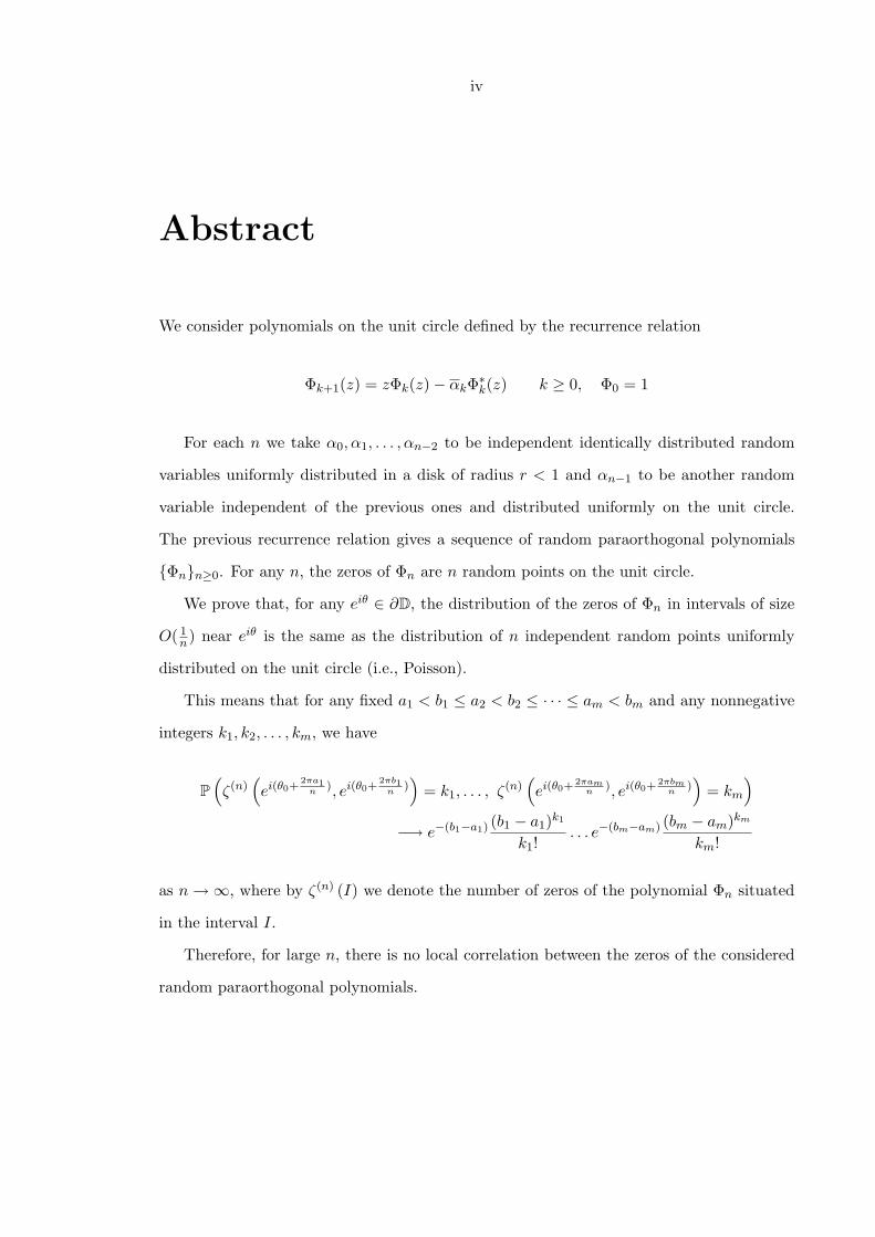
We consider polynomials on the unit circle defined by the recurrence relation

Φk+1(z) = zΦk(z)− αkΦ∗k(z) k ≥ 0, Φ0 = 1

For each n we take α0, α1, . . . , αn−2 to be independent identically distributed random

variables uniformly distributed in a disk of radius r < 1 and αn−1 to be another random

variable independent of the previous ones and distributed uniformly on the unit circle.

The previous recurrence relation gives a sequence of random paraorthogonal polynomials

Φnn≥0. For any n, the zeros of Φn are n random points on the unit circle.

We prove that, for any eiθ ∈ ∂D, the distribution of the zeros of Φn in intervals of size

O( 1n) near eiθ is the same as the distribution of n independent random points uniformly

distributed on the unit circle (i.e., Poisson).

This means that for any fixed a1 < b1 ≤ a2 < b2 ≤ · · · ≤ am < bm and any nonnegative

integers k1, k2, . . . , km, we have

P(ζ(n)

(ei(θ0+

2πa1n

), ei(θ0+2πb1

n))

= k1, . . . , ζ(n)(ei(θ0+ 2πam

n), ei(θ0+ 2πbm

n))

= km

)

−→ e−(b1−a1) (b1 − a1)k1

k1!. . . e−(bm−am) (bm − am)km

km!

as n →∞, where by ζ(n) (I) we denote the number of zeros of the polynomial Φn situated

in the interval I.

Therefore, for large n, there is no local correlation between the zeros of the considered

random paraorthogonal polynomials.

v

The same result holds when we take α0, α1, . . . , αn−2 to be independent identically

distributed random variables uniformly distributed in a circle of radius r < 1 and αn−1 to

be another random variable independent of the previous ones and distributed uniformly on

the unit circle.

vi

Contents

Acknowledgements iii

Abstract iv

1 Introduction 1

1.1 Outline of the Proof of the Main Theorem . . . . . . . . . . . . . . . . . . . 11

2 Background on OPUC 15

2.1 Definition, Basic Properties, Examples . . . . . . . . . . . . . . . . . . . . . 15

2.2 Zeros of OPUC and POPUC . . . . . . . . . . . . . . . . . . . . . . . . . . 17

2.3 The CMV Matrix and Its Resolvent, Dynamical Properties of the CMV Ma-

trices . . . . . . . . . . . . . . . . . . . . . . . . . . . . . . . . . . . . . . . . 21

2.4 Properties of Random CMV Matrices . . . . . . . . . . . . . . . . . . . . . 26

3 Background on Random Schrodinger Operators 31

3.1 The Anderson Model . . . . . . . . . . . . . . . . . . . . . . . . . . . . . . . 31

3.2 The Statistical Distribution of the Eigenvalues for the Anderson Model: The

Results of Molchanov and Minami . . . . . . . . . . . . . . . . . . . . . . . 38

4 Aizenman-Molchanov Bounds for the Resolvent of the CMV Matrix 43

4.1 Uniform Bounds for the Fractional Moments . . . . . . . . . . . . . . . . . 43

4.2 The Uniform Decay of the Expectations of the Fractional Moments . . . . . 47

4.3 The Exponential Decay of the Fractional Moments . . . . . . . . . . . . . . 52

5 Spectral Properties of Random CMV Matrices 60

vii

5.1 The Localized Structure of the Eigenfunctions . . . . . . . . . . . . . . . . . 60

5.2 Decoupling the CMV Matrices . . . . . . . . . . . . . . . . . . . . . . . . . 63

6 The Local Statistical Distribution of the Zeros of Random Paraorthogonal

Polynomials 70

6.1 Estimating the Probability of Having Two or More Eigenvalues in an Interval 70

6.2 Proof of the Main Theorem . . . . . . . . . . . . . . . . . . . . . . . . . . . 76

6.3 The Case of Random Verblunsky Coefficients Uniformly Distributed on a Circle 77

7 Appendices 82

Bibliography 87

1

Chapter 1

Introduction

In this thesis we study orthogonal polynomials on the unit circle given by random Verblun-

sky coefficients. More precisely, we will consider random paraorthogonal polynomials (which

have their zeros on the unit circle) and we will describe the statistical distribution of these

zeros.

For any sequence of complex numbers αnn≥0 we can consider the sequence of polyno-

mials Φnn≥0 defined by Φ0 = 1 and by the recurrence relation

Φk+1(z) = zΦk(z)− αkΦ∗k(z) k ≥ 0, (1.0.1)

where for any k > 0, Φ∗k(z) = zk Φk(1z ) (or, equivalently, if Φk(z) =

∑kj=0 ajz

j , then

Φ∗k(z) =∑k

j=0 ak−j zj).

Henceforth, we will denote by D the unit disk and by ∂D the unit circle.

Consider a nontrivial (i.e., not supported on a finite set) probability measure on the unit

circle. Then the sequence of polynomials 1, z, z2, . . . is in L2(∂D, dµ). Since the measure µ

is nontrivial, the polynomials 1, z, z2, . . . are linearly independent. We can apply the Gram-

Schmidt process to this sequence and get a sequence of orthogonal monic polynomials

Φ0,Φ1, . . .. It is easy to see that these polynomials obey the recurrence relation (1.0.1),

where the complex numbers αnn≥0 satisfy |αn| < 1 for any n.

Theorem 1.0.1 (Verblunsky). There is a bijection between nontrivial (i.e., not supported

on a finite set) probability measures on the unit circle and sequences of complex numbers

αnn≥0 with |αn| < 1 for any n.

2

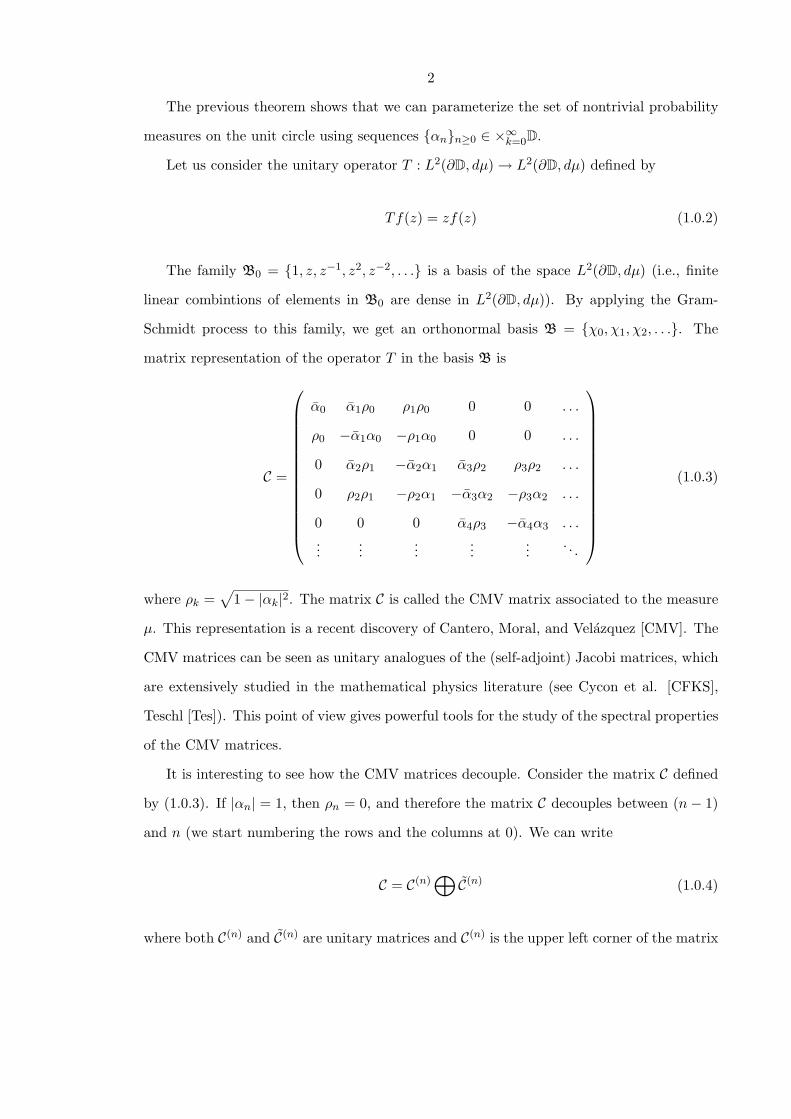
The previous theorem shows that we can parameterize the set of nontrivial probability

measures on the unit circle using sequences αnn≥0 ∈ ×∞k=0D.

Let us consider the unitary operator T : L2(∂D, dµ) → L2(∂D, dµ) defined by

Tf(z) = zf(z) (1.0.2)

The family B0 = 1, z, z−1, z2, z−2, . . . is a basis of the space L2(∂D, dµ) (i.e., finite

linear combintions of elements in B0 are dense in L2(∂D, dµ)). By applying the Gram-

Schmidt process to this family, we get an orthonormal basis B = χ0, χ1, χ2, . . .. The

matrix representation of the operator T in the basis B is

C =

α0 α1ρ0 ρ1ρ0 0 0 . . .

ρ0 −α1α0 −ρ1α0 0 0 . . .

0 α2ρ1 −α2α1 α3ρ2 ρ3ρ2 . . .

0 ρ2ρ1 −ρ2α1 −α3α2 −ρ3α2 . . .

0 0 0 α4ρ3 −α4α3 . . .

......

......

.... . .

(1.0.3)

where ρk =√

1− |αk|2. The matrix C is called the CMV matrix associated to the measure

µ. This representation is a recent discovery of Cantero, Moral, and Velazquez [CMV]. The

CMV matrices can be seen as unitary analogues of the (self-adjoint) Jacobi matrices, which

are extensively studied in the mathematical physics literature (see Cycon et al. [CFKS],

Teschl [Tes]). This point of view gives powerful tools for the study of the spectral properties

of the CMV matrices.

It is interesting to see how the CMV matrices decouple. Consider the matrix C defined

by (1.0.3). If |αn| = 1, then ρn = 0, and therefore the matrix C decouples between (n− 1)

and n (we start numbering the rows and the columns at 0). We can write

C = C(n)⊕

C(n) (1.0.4)

where both C(n) and C(n) are unitary matrices and C(n) is the upper left corner of the matrix

3

C. The n× n matrix C(n) will be called the truncated CMV matrix.

Recall that the orthogonal polynomials Φ0, Φ1, . . . were obtained by applying the Gram-

Schmidt process to the sequence 1, z, . . . in the space L2(∂D, dµ) (µ is a nontrivial measure,

i.e., suppµ is infinite). In this situation we have |αk| < 1 for any k. On the other hand,

the case α0, α1, . . . αn−1 ∈ D and |αn| = 1 corresponds to the situation when the Gram-

Schmidt process stops. In this situation, the support of the measure µ is finite and the

space L2(∂D, dµ) is finite-dimensional. For any k ∈ 1, . . . , n− 1, the zeros of Φk are in D.

The zeros of the polynomial Φn are on ∂D. It is not hard to see that the zeros of Φn are

exactly the eigenvalues of the matrix C(n) defined in (1.0.4).

The polynomials Φn obtained by the recurrence relation (1.0.1) with α0, α1, . . . , αn−2 ∈D and with αn−1 ∈ ∂D are called by some authors paraorthogonal polynomials. Their zeros

are used in the quadrature theorem of Jones, Njastad, and Thron [JNT].

Before we state this theorem we should define the Christoffel coefficients associated to

a measure µ at a point z ∈ C to be

λn(z, µ) = min∫

∂D|π(eiθ)|2dµ(θ)

∣∣∣ π polynomial , deg π ≤ n, π(z) = 1

(1.0.5)

Theorem 1.0.2 (Jones, Njastad, Thron). Let µ be a nontrivial probability measure on

the unit circle and αnn≥0 the set of corresponding Verblunsky coefficients. Let β1, β2, . . .

be a sequence of points on the unit circle and Φn+1 the paraorthogonal polynomial obtained

from the coefficients α0, α1, . . . , αn−1, βn. Let z(n+1)1 , z

(n+1)2 , . . . , z

(n+1)n+1 be the zeros of the

polynomial Φn+1 and

µn+1(βn) =n+1∑

k=1

λn(z(n+1)k , µ) δ

z(n+1)k

(1.0.6)

where the λn(z(n+1)k , µ) are the Christoffel coefficients corresponding to the measure µ and

the points λn(z(n+1)k , µ).

Then, for any choice of β1, β2, . . ., the sequence of measures µn+1(βn) converges weakly

to µ.

We will sometimes use the abbreviations OPUC for orthogonal polynomials on the unit

circle and POPUC for paraorthogonal polynomials on the unit circle.

4

We will consider random paraorthogonal polynomials (i.e., paraorthogonal polynomials

defined by random recurrence coefficients α0, α1, . . . , αn−2 ∈ D and β ∈ ∂D). We will study

the distribution of the zeros of the paraorthogonal polynomials as n →∞. As we have seen

before, this is equivalent to the study of the distribution of the eigenvalues of the truncated

CMV matrices.

It will be useful to view the random points on the unit circle as a point process (for

a general introduction to the theory of point processes, see [DVJ03]). Let X be a fixed

topological space (X will be R or ∂D). We define by M(X) the space of all nonnegative

Radon measures on X. Let also Mp(X) be the space of all integer-valued Radon measures

on X. Clearly any measure ζ ∈Mp(X) can be written as

ζ =∑

k

δζk(1.0.7)

where the sum is finite or countable, ζk ∈ X for any k, and the set ζk has no accumulation

point in X. As usual, we endow the space M(X) with the vague topology and Mp(X) with

the topology induced from M(X). Let’s also fix a probability space (Ω,P).

By definition, a point process is a measurable function

ζ = ζ(ω) : Ω →Mp(X) (1.0.8)

It is clear that for any Borel set A ⊂ X, we can define a random variable

ζ(A) : Ω → Z (1.0.9)

defined by ζ(A)(ω) = ζ(ω)(A) (i.e., the number of points ζ(ω) has in the set A).

We say that the point process ζ has the intensity measure µ if and only if, for any Borel

set A, we have

µ(A) = E (ζ(A)) (1.0.10)

It is clear that the study of any point process is equivalent to the study of the integer-

valued random variables ζ(A) for Borel sets A ⊂ X.

5

One of the most important point processes is the Poisson point process. Let’s fix a

measure µ on the real line. By definition, the Poisson point process with intensity measure

µ is the point process ζ : Ω →Mp(X), which obeys the following:

i) For any Borel set A ⊂ X, the random variable ζ(A) has a Poisson distribution with

intensity measure µ(A). This means that for any nonnegative integer k,

P(ζ(A) = k) = e−µ(A) µ(A)k

k!(1.0.11)

ii) If the A1, A2, . . . , Am are disjoint Borel subsets of X, then ζ(A1), ζ(A2), . . . , ζ(Am)

are independent random variables.

The Poisson distribution for a collection of random points indicates the fact that the

points are completely independent in the space X (i.e., they don’t “see” each other). This

means that there is no correlation (attraction or repulsion) between these points. An

elementary introduction to the theory of Poisson processes is [Kin].

We will want to prove that a sequence of point processes ζ(n) on the probability space

(Ω,P) converges to the Poisson point process and therefore to conclude that there is no

correlation between points as n →∞. In order to do this, we should first define the notion

of limit of a sequence of point processes.

Consider another point process ζ on a probability space (Ω, P). By definition, we say

that ζn converges (weakly) to ζ if and only if, for any bounded continuous function F :

Mp(X) → C, we have

limn→∞

∫

ΩF (ζ(ω))P(ω) =

∫

ΩF (ζ(ω))P(ω) (1.0.12)

A very important problem in mathematical physics is the study of the statistical distri-

bution of the eigenvalues of some classes of (n×n) random matrices (self-adjoint or unitary).

For any n we will denote by ζ(n) the point process obtained by taking a Dirac measure of

mass 1 at any eigenvalue of the (n × n) matrix considered. For this situation it would be

meaningless to study the random variables ζ(n)(A). This is because for any fixed set A with

P(A) > 0, the expectation of the random variable ζ(n)(A) will converge to ∞ as n → ∞.

6

Instead, we should rescale the set A by a factor of n for every value of n. We will do this

in the following way: We will first fix a point x ∈ X and a set A ⊂ X. Then, for any n, we

will rescale the set A near the point x by a factor of n and get a set A(n) of measure O( 1n).

We will then study the random variables ζ(n)(A(n)) as n →∞.

For example, if X = R, then, for a point r ∈ R and an interval A = (a, b) ⊂ R, we will

have A(n) = (r + an , r + b

n). In the case X = ∂D, for a point eiθ ∈ ∂D and an interval (arc)

A = (eia, eib), we have A(n) = (ei(θ+ 2πan

), ei(θ+ 2πbn

)).

We will say that the rescaled (by the factor n) point process ζ(n) converges locally to the

Poisson point process with the intensity measure µ near the point p ∈ X (which is r ∈ R in

the first case and eiθ ∈ ∂D in the second case) if and only if

i) For any disjoint A1, A2, . . . , Am ∈ X, the random variables ζ(n)(A(n)1 ), ζ(n)(A(n)

2 ), . . .,

ζ(n)(A(n)m ) are independent;

ii) For any fixed a1 < b1 ≤ a2 < b2 ≤ · · · ≤ am < bm and any nonnegative integers

k1, k2, . . . , km, we have, in the first case (X = R, r ∈ R):

P(

ζ(n)

(r +

a1

n, r +

b1

n

)= k1, . . . , ζ(n)

(r +

am

n, r +

bm

n

)= km

)

−→ e−µ((a1,b1)) µ((a1, b1))k1

k1!. . . e−µ((am,bm)) µ((am, bm))km

km!(1.0.13)

as n →∞.

In the second case (X = ∂D, eiθ ∈ ∂D):

P(ζ(n)

(ei(θ+

2πa1n

), ei(θ+2πb1

n))

= k1, . . . , ζ(n)(ei(θ+ 2πam

n), ei(θ+ 2πbm

n))

= km

)

−→ e−µ((a1,b1)) µ((a1, b1))k1

k1!. . . e−µ((am,bm)) µ((am, bm))km

km!(1.0.14)

as n →∞.

As mentioned earlier, we will consider random n × n truncated CMV matrices. For

any n, we define, as before, the point process ζ(n). Since the truncated CMV matrices are

unitary, ζ(n) is a point process on the unit circle. We will prove that for any eiθ ∈ ∂D,

the sequence ζ(n) converges locally (on intervals of size O( 1n) near eiθ) to a Poisson point

7

process.

We will now set the stage for this result.

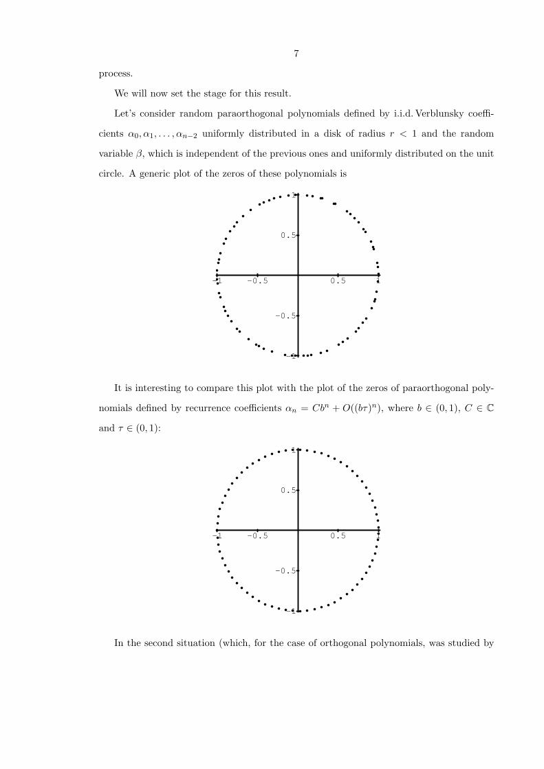
Let’s consider random paraorthogonal polynomials defined by i.i.d. Verblunsky coeffi-

cients α0, α1, . . . , αn−2 uniformly distributed in a disk of radius r < 1 and the random

variable β, which is independent of the previous ones and uniformly distributed on the unit

circle. A generic plot of the zeros of these polynomials is

0.5 1-0.5-1

0.5

1

-0.5

-1

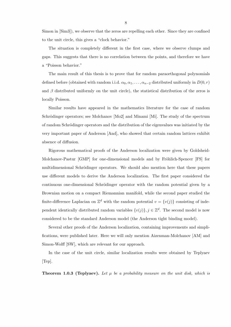
It is interesting to compare this plot with the plot of the zeros of paraorthogonal poly-

nomials defined by recurrence coefficients αn = Cbn + O((bτ)n), where b ∈ (0, 1), C ∈ Cand τ ∈ (0, 1):

0.5 1-0.5-1

0.5

1

-0.5

-1

In the second situation (which, for the case of orthogonal polynomials, was studied by

8

Simon in [Sim3]), we observe that the zeros are repelling each other. Since they are confined

to the unit circle, this gives a “clock behavior.”

The situation is completely different in the first case, where we observe clumps and

gaps. This suggests that there is no correlation between the points, and therefore we have

a “Poisson behavior.”

The main result of this thesis is to prove that for random paraorthogonal polynomials

defined before (obtained with random i.i.d. α0, α1, . . . , αn−2 distributed uniformly in D(0, r)

and β distributed uniformly on the unit circle), the statistical distribution of the zeros is

locally Poisson.

Similar results have appeared in the mathematics literature for the case of random

Schrodinger operators; see Molchanov [Mo2] and Minami [Mi]. The study of the spectrum

of random Schrodinger operators and the distribution of the eigenvalues was initiated by the

very important paper of Anderson [And], who showed that certain random lattices exhibit

absence of diffusion.

Rigorous mathematical proofs of the Anderson localization were given by Goldsheid-

Molchanov-Pastur [GMP] for one-dimensional models and by Frohlich-Spencer [FS] for

multidimensional Schrodinger operators. We should also mention here that these papers

use different models to derive the Anderson localization. The first paper considered the

continuous one-dimensional Schrodinger operator with the random potential given by a

Brownian motion on a compact Riemannian manifold, while the second paper studied the

finite-difference Laplacian on Zd with the random potential v = v(j) consisting of inde-

pendent identically distributed random variables v(j), j ∈ Zd. The second model is now

considered to be the standard Anderson model (the Anderson tight binding model).

Several other proofs of the Anderson localization, containing improvements and simpli-

fications, were published later. Here we will only mention Aizenman-Molchanov [AM] and

Simon-Wolff [SW], which are relevant for our approach.

In the case of the unit circle, similar localization results were obtained by Teplyaev

[Tep].

Theorem 1.0.3 (Teplyaev). Let µ be a probability measure on the unit disk, which is

9

absolutely continuous with respect to the Lebesgue measure, and

∫

Dlog(1− |x|) dµ(x) > −∞

Consider a sequence of independent identically distributed random variables a0, a1, . . . with

the probability distribution µ. Let σ = σ(a0, a1, . . .) be the random probability measure on

the unit circle given by the Verblunsky’s theorem. Then, with probability 1, σ is a pure point

measure.

A recent important development in the theory of orthogonal polynomials on the unit

circle was obtained by Golinskii and Nevai in [GN]. In this paper the authors use transfer

matrices and the theory of subordinate solutions (some of the key ingredients in the mod-

ern theory of Schrodinger operators) to investigate the spectral measures corresponding to

orthogonal polynomials on the unit circle.

In addition to the phenomenon of localization, one can also analyze the local structure

of the spectrum. It turns out that, for the case of the Schrodinger operator, there is no

repulsion between the energy levels. This was shown by Molchanov [Mo2] for the model of

the one-dimensional Schrodinger operator studied by the Russian school.

Theorem 1.0.4 (Molchanov). For any V > 0, consider the one-dimensional Schrodinger

operator on L2((−V, V )),

HV = − d2

dt2+ q(t, ω)

with Dirichlet boundary conditions. The random potential q(t, ω) has the form q(t, ω) =

F (xt) where xt is a Brownian motion on a compact Riemannian manifold K and F : K →R is a smooth Morse function with minx∈K F (x) = 0. Denote by NV (I) the number of

eigenvalues of the operator HV situated in the interval I. Let E0 > 0 and n(E0) the limit

density of states of the operator HV as V →∞. Then:

limV→∞

P(NV

(E0 − a

2V, E0 +

a

2V

))−→ e−a n(E0) (an(E0))k

k!

Using the terminology of point processes presented before, this means that the local

10

statistical distribution of the eigenvalues of the operator HV (rescaled near E0) converges,

as V → ∞, to the Poisson point process with intensity measure n(E0)dx (here dx denotes

the Lebesgue measure).

The case of the multidimensional discrete Schrodinger operator was analyzed by Minami

in [Mi].

Theorem 1.0.5 (Minami). Consider the Anderson tight binding model

H = −∆ + V (ω)

and denote by HΛ its restriction to hypercubes Λ ⊂ Zd. Let E ∈ R be an energy for which

the Aizenman-Molchanov bounds (3.1.17) hold (see also Theorem 3.1.9) and denote by n(E)

the density of states at E. For any hypercube Λ, let Ej(Λ)j, j ≥ 1 be the eigenvalues of

the operator HΛ and let

ζj(Λ, E) = |Λ|(Ej(Λ)−E)

be its rescaled eigenvalues. Then the point process ζ(Λ) = ζj(Λ, E)j converges to the

Poisson point process with intensity measure n(E)dx as the box Λ gets large (Λ ↑ Zd).

Both in Theorems 1.0.4 and 1.0.5, Molchanov and Minami proved that the statisti-

cal distribution of the rescaled eigenvalues converges locally to a stationary Poisson point

process. This means that there is no correlation between eigenvalues.

We will use some techniques from the spectral theory of discrete Schrodinger operators

to study the distribution of the zeros of the random paraorthogonal polynomials, especially

ideas and methods developed in [AM]. However, our model on the unit circle has many dif-

ferent features compared to the discrete Schrodinger operator (perhaps the most important

one is that we have to consider unitary operators on the unit circle instead of self-adjoint

operators on the real line). Therefore, we will have to use new ideas and techniques that

work for this situation (see [Sto]).

The final goal is the following:

Theorem 1.0.6 (Main Theorem). Consider the random polynomials on the unit circle

11

given by the following recurrence relations:

Φk+1(z) = zΦk(z)− αkΦ∗k(z) k ≥ 0, Φ0 = 1 (1.0.15)

where α0, α1, . . . , αn−2 are i.i.d. random variables distributed uniformly in a disk of radius

r < 1, and αn−1 is another random variable independent of the previous ones and uniformly

distributed on the unit circle.

Consider the space Ω = α = (α0, α1, . . . , αn−2, αn−1) ∈ D(0, r) × D(0, r) × · · · ×D(0, r)× ∂D with the probability measure P obtained by taking the product of the uniform

(Lebesgue) measures on each D(0, r) and on ∂D. Fix a point eiθ0 ∈ D and let ζ(n) be the

point process defined previously (by taking a Dirac measure of mass 1 at any eigenvalue of

the matrix C(n)).

Then, on a fine scale (of order 1n) near eiθ0, the point process ζ(n) converges to the

Poisson point process with intensity measure n dθ2π (where dθ

2π is the normalized Lebesgue

measure). This means that for any fixed a1 < b1 ≤ a2 < b2 ≤ · · · ≤ am < bm and any

nonnegative integers k1, k2, . . . , km, we have

P(ζ(n)

(ei(θ0+

2πa1n

), ei(θ0+2πb1

n))

= k1, . . . , ζ(n)(ei(θ0+ 2πam

n), ei(θ0+ 2πbm

n))

= km

)

−→ e−(b1−a1) (b1 − a1)k1

k1!. . . e−(bm−am) (bm − am)km

km!(1.0.16)

as n →∞.

1.1 Outline of the Proof of the Main Theorem

From now on we will work under the hypotheses of Theorem 1.0.6. We will study the

statistical distribution of the eigenvalues of the random CMV matrices

C(n) = C(n)α (1.1.1)

for α ∈ Ω (with the space Ω defined in Theorem 1.0.6).

A first step in the study of the spectrum of random CMV matrix is proving the exponen-

12

tial decay of the fractional moments of the resolvent of the CMV matrix. These ideas were

developed in the case of Anderson models by Aizenman-Molchanov [AM] and by Aizenman

et al. [ASFH]; they provide a powerful method for proving spectral localization, dynamical

localization, and the absence of level repulsion.

Before we state the Aizenman-Molchanov bounds, we have to make a few remarks on

the boundary behavior of the matrix elements of the resolvent of the CMV matrix. For any

z ∈ D and any 0 ≤ k, l ≤ (n− 1), we will use the following notation:

Fkl(z, C(n)α ) =

[C(n)

α + z

C(n)α − z

]

kl

(1.1.2)

As we will see in the next section, using properties of Caratheodory functions, we will

get that for any α ∈ Ω, the radial limit

Fkl(eiθ, C(n)α ) = lim

r↑1Fkl(reiθ, C(n)

α ) (1.1.3)

exists for Lebesgue almost every eiθ ∈ ∂D and Fkl( · , C(n)α ) ∈ Ls(∂D) for any s ∈ (0, 1).

Since the distributions of α0, α1, . . . , αn−1 are rotationally invariant, we obtain that for any

fixed eiθ ∈ ∂D, the radial limit Fkl(eiθ, C(n)α ) exists for almost every α ∈ Ω. We can also

define

Gkl(z, C(n)α ) =

[1

C(n)α − z

]

kl

(1.1.4)

and

Gkl(eiθ, C(n)α ) = lim

r↑1Gkl(reiθ, C(n)

α ) (1.1.5)

Using the previous notation, we have

Theorem 1.1.1 (Aizenman-Molchanov Bounds for the Resolvent of the CMV

Matrix). For the model considered in Theorem 1.0.6 and for any s ∈ (0, 1), there exist

constants C1, D1 > 0 such that for any n > 0, any k, l, 0 ≤ k, l ≤ n− 1, and any eiθ ∈ ∂D,

13

we have

E(∣∣∣Fkl(eiθ, C(n)

α )∣∣∣s)≤ C1 e−D1|k−l| (1.1.6)

where C(n) is the (n × n) CMV matrix obtained for α0, α1, . . . , αn−2 uniformly distributed

in D(0, r) and αn−1 uniformly distributed in ∂D.

Using Theorem 1.1.1, we will then be able to control the structure of the eigenfunctions

of the matrix C(n).

Theorem 1.1.2 (The Localized Structure of the Eigenfunctions). For the model

considered in Theorem 1.0.6, the eigenfunctions of the random matrices C(n) = C(n)α are

exponentially localized with probability 1, that is, exponentially small outside sets of size

proportional to (lnn). Hence there exists a constant D2 > 0, and for almost every α ∈ Ω,

there exists a constant Cα > 0 such that for any unitary eigenfunction ϕ(n)α , there exists

a point m(ϕ(n)α ) (1 ≤ m(ϕ(n)

α ) ≤ n) with the property that for any m, |m − m(ϕ(n)α )| ≥

D2 ln(n + 1), we have

|ϕ(n)α (m)| ≤ Cα e−(4/D2) |m−m(ϕ

(n)α )| (1.1.7)

The point m(ϕ(n)α ) will be taken to be the smallest integer where the eigenfunction

ϕ(n)α (m) attains its maximum absolute value.

In order to obtain a Poisson distribution in the limit as n →∞, we will use the approach

of Molchanov [Mo2] and Minami [Mi]. The first step is to decouple the point process ζ(n) into

the direct sum of smaller point processes. We will do the decoupling process in the following

way: For any positive integer n, let C(n) be the CMV matrix obtained for the coefficients

α0, α1, . . . , αn with the additional restrictions α[ nln n ] = eiη1 , α2[ n

ln n ] = eiη2 , . . . , αn = eiη[ln n] ,

where eiη1 , eiη2 , . . . , eiη[ln n] are independent random points uniformly distributed on the unit

circle. Note that the matrix C(n) decouples into the direct sum of ≈ [ln n] unitary matrices

C(n)1 , C(n)

2 , . . . , C(n)[ln n]. We should note here that the actual number of blocks C(n)

i is slightly

larger than [lnn] and that the dimension of one of the blocks (the last one) could be smaller

than[

nln n

].

However, since we are only interested in the asymptotic behavior of the distribution

14

of the eigenvalues, we can, without loss of generality, work with matrices of size N =

[ln n][

nln n

]. The matrix C(N) is the direct sum of exactly [lnn] smaller blocks C(N)

1 , C(N)2 ,

. . . , C(N)[ln n]. Let’s define ζ(N,p) =

∑[n/ ln n]k=1 δ

z(p)k

where z(p)1 , z

(p)2 , . . . , z

(p)[n/ ln n] are the eigenvalues

of the matrix C(N)p . The decoupling result is formulated in the following theorem:

Theorem 1.1.3. The point process ζ(N) can be asymptotically approximated by the direct

sum of point processes∑[ln n]

p=1 ζ(N,p). In other words, the distribution of the eigenvalues of

the matrix C(N) can be asymptotically approximated by the distribution of the eigenvalues of

the direct sum of the matrices C(N)1 , C(N)

2 , . . . , C(N)[ln n].

The decoupling property is the first step in proving that the statistical distribution of

the eigenvalues of C(N) is Poisson. In the theory of point processes (see, e.g., Daley and

Vere-Jones [DVJ88]), a point process obeying this decoupling property is called an infinitely

divisible point process. In order to show that this distribution is Poisson on a scale of order

O( 1n) near a point eiθ, we need to check two conditions:

i)[ln n]∑

p=1

P(ζ(N,p) (A (N, θ)) ≥ 1

)→ |A| as n →∞ (1.1.8)

ii)[ln n]∑

p=1

P(ζ(N,p) (A (N, θ)) ≥ 2

)→ 0 as n →∞ (1.1.9)

where for an interval A = [a, b] we define A(N, θ) = (ei(θ+ 2πaN

), ei(θ+ 2πbN

)) and | · | is the

Lebesgue measure (and we extend this definition to unions of intervals). The second condi-

tion shows that it is asymptotically impossible that any of the matrices C(N)1 , C(N)

2 , . . . , C(N)[ln n]

has two or more eigenvalues situated in an interval of size 1N . Therefore, each of the matri-

ces C(N)1 , C(N)

2 , . . . , C(N)[ln n] contributes at most one eigenvalue in an interval of size 1

N . But

the matrices C(N)1 , C(N)

2 , . . . , C(N)[ln n] are decoupled, hence independent, and therefore we get

a Poisson distribution. Condition i) now gives Theorem 1.0.6.

15

Chapter 2

Background on OPUC

In this chapter we will present a few basic results in the theory of orthogonal polynomials

on the unit circle. Special attention will be devoted to the zeros of these polynomials and

to the CMV matrices. We will also introduce some of the main tools used in the study of

these mathematical objects. Most of the results and proofs of the theorems stated in this

chapter can be found in [Sim4] and [Sim5].

2.1 Definition, Basic Properties, Examples

As explained in Chapter 1, for any nontrivial probability measure µ on ∂D, defining

the infinite-dimensional Hilbert space L2(∂D, dµ), the orthonormal polynomials ϕ0(z, µ),

ϕ1(z, µ), ϕ2(z, µ), . . . are obtained by applying the Gram-Schmidt process to the sequence

of polynomials 1, z, z2, . . .. For any n ≥ 0, we can define the corresponding monic polynomial

Φn(z, µ) =1κn

ϕn(z, µ) (2.1.1)

(where by κn we denote the leading coefficient of the polynomial ϕn(z, µ)).

The monic polynomials Φn(z, µ)n≥0 obey the recurrence relation

Φn+1(z) = z Φn(z)− αn Φ∗n(z) n ≥ 0 (2.1.2)

where for any n ≥ 0, we have αn ∈ D. The complex numbers αn are called the Verblunsky

coefficients associated to the measure µ.

16

Verblunsky’s theorem (Theorem 1.0.1) states that there is a bijection between nontrivial

measures µ on the unit circle and sequences of complex numbers αnn≥0 ⊂ D. One of the

most important questions in the theory of orthogonal polynomials on the unit circle is how

properties of the measure µ correspond to properties of the Verblunsky coefficients αnn≥0

and vice-versa.

Two very important tools in the study of orthogonal polynomials on the unit circle

are the Caratheodory and the Schur functions associated to the spectral measure µ. The

Caratheodory function is defined for z ∈ D by the relation:

F (z) =∫

∂D

eiθ + z

eiθ − zdµ(θ) (2.1.3)

Note that F is analytic on D, F (0) = 1, and ReF (z) ≥ 0 for any z ∈ D.

The Schur function f : D→ C, is corresponding to the measure µ, can be obtained from

the Caratheodory function F using the relation

f(z) =1z

F (z)− 1F (z) + 1

(2.1.4)

Note that the function f is analytic and |f(z)| ≤ 1 for any z ∈ D.

A few important examples of orthogonal polynomials on the unit circle are

1. The Free Case: µ = dθ2π (the normalized Lebesgue measure). In this case we have

αn = 0 for any n, F (z) = 1, and f(z) = 0.

2. Bernstein-Szego Polynomials with Parameter ζ = reiθ ∈ D: µ = Pr(θ, ϕ) dθ2π , where

Pr(θ, ϕ) =1− r2

1 + r2 − 2r cos(θ − ϕ)

is the Poisson kernel. In this case we have α0 = reiθ and αn = 0 for any n ≥ 1. Also

F (z) = 1+zζ1−zζ and f(z) = ζ.

3. Single Inserted Mass Point with Parameter γ ∈ (0, 1): µ = (1− γ) dθ2π + γδ(θ − 0). In

this case αn = γ1+nγ , F (z) = 1−(1−2γ)z

1−z , and f(z) = γ1−(1−γ)z .

4. Geronimus Polynomials with Parameter α ∈ D: µ = w(θ) dθ2π + µs, where for the

17

auxiliary parameter β defined by 1 + α = |1 + α|eiβ/2, we have

w(θ) =

1|1+α|

√cos2(arcsin(|α|))−cos2(θ/2)

sin((θ−β)/2) , θ ∈ (2 arcsin(|α|, 2π − 2 arcsin(|α|))0, θ ∈ [−2 arcsin(|α|), 2 arcsin(|α|)]

(2.1.5)

and

µs =

0, if |α + 12 | ≤ 1

2 ;

2|1+α|2 (|α + 1

2 |2 − 14)δ(θ − β), if |α + 1

2 | > 12

(2.1.6)

In this case we have αn = α for any n ≥ 0. The formulae for the Caratheodory and

Schur functions are more complicated:

F (z) = 1 +2

(z + 1 +

√(z − e2i arcsin(|α|))(z − e−2i arcsin(|α|)) + αz − 1

)

1 + α− (1− α)z(2.1.7)

and

f(z) =z + 1 +

√(z − e2i arcsin(|α|))(z − e−2i arcsin(|α|))− 2

2αz(2.1.8)

More examples of orthogonal polynomials on the unit circle are presented in Section 1.6

of [Sim4].

2.2 Zeros of OPUC and POPUC

One of the central questions in the theory of orthogonal polynomials on the unit circle is to

understand the location of the zeros of Φn(z, µ).

We will start with the basic theorems:

Theorem 2.2.1 (Zeros Theorem for OPUC). Let Φn(z, µ) be the n-th degree monic

orthogonal polynomial corresponding to the measure µ. Then all the zeros of Φn(z, µ) lie in

D.

As explained in Chapter 1, for any nontrivial probability measure µ with the Verblunsky

coefficients αkk≥0 and the orthogonal polynomials Φk(z, µ)k≥0, any n ≥ 0 and any

18

β ∈ ∂D, we can define the paraorthogonal polynomials

Φn+1(z, µ, β) = zΦn(z, µ) + βΦ∗n(z, µ) (2.2.1)

For the zeros of paraorthogonal polynomials we have

Theorem 2.2.2 (Zeros Theorem for POPUC). Let Φn(z, µ, β) be the n-th degree monic

paraorthogonal polynomial defined before. Then all the zeros of Φn(z, µ, β) lie in ∂D.

The proofs of Theorems 2.2.1 and 2.2.2 can be found in [Sim4].

We will now present a few results about the zeros of OPUC and later turn our attention

to zeros of POPUC. One of the first questions that can be asked is whether any countable

set of points in D can be the zeros of orthogonal polynomials. The answer is positive and

is given by the following:

Theorem 2.2.3 (Alfaro-Vigil [AlVi]). Let znn≥1 be a sequence of complex numbers of

absolute value strictly less than 1. Then there exists a unique nontrivial probability measure

µ with Φn(zn, µ) = 0.

A clear limitation of the previous theorem is that we can only prescribe one zero for

each orthogonal polynomial. It is natural to ask whether we can prescribe more zeros for

the polynomial Φn. The answer is again positive and was recently discovered by Simon and

Totik:

Theorem 2.2.4 (Simon-Totik [ST]). Let znn≥1 be a sequence of complex numbers of

absolute value strictly less than 1 and let 0 < m1 < m2 < m3 < · · · be any increasing

sequence of positive numbers. Then there exists a nontrivial probability measure µ on ∂D

with

Φmj (zk, µ) = 0 k = mj−1 + 1, . . . , mj (2.2.2)

Another question that one can ask is whether the particular properties of the measure

µ can influence the location of the zeros of the orthogonal polynomials. It turns out that

the zeros of the orthogonal polynomials can only be located in the convex hull of supp(µ).

19

Theorem 2.2.5 (Fejer). Let µ be a nontrivial measure on ∂D and let Φn(z, µ) be the

corresponding monic polynomials associated to this measure. Then all the zeros of Φn(z, µ)

lie in the interior of the convex hull of supp(µ).

It is worth mentioning that the previous theorem holds for arbitrary nontrivial measures

in C.

The zeros of paraorthogonal polynomials on the unit circle were studied by Golinskii in

[Gol]. We will list here the main results obtained in this paper. As before, we fix a nontrivial

probability measure µ on ∂D with Verblunsky coefficients αnn≥0 and orthogonal polyno-

mials Φn(z, µ)n≥0. For a fixed complex number β ∈ ∂D, we consider the paraorthogonal

polynomials Φn(z, µ, β)n≥0.

For any n, denote by zn,k0≤k≤(n−1) the zeros of the polynomial Φn(z, µ, β) (they are

situated on the unit circle). We order the numbers zn,k such that for any k, the point zn,k

is between zn,(k−1) and zn,(k+1) (with the convention zn,n = zn,0). Note that the ordering is

unique once we fix the starting point, zn,0.

Theorem 2.2.6. For any integer n ≥ 2, there exists particular orderings of the zeros of

the polynomials Φn(z, µ, β) and Φn+1(z, µ, β) such that the sets S1 = zn,k0≤k≤(n−1) and

S2 = zn+1,k1≤k≤n are alternating (i.e., between each two adjacent points of either of them,

there is exactly one point of the other).

It is also interesting to control the distance between the zeros of the polynomials

Φn(z, µ, β) in terms of the measure µ. Suppose that the Lebesgue decomposition of the

spectral measure µ is µ = f(θ) dθ2π + µs. Then we have the following:

Theorem 2.2.7. If log f ∈ L1(∂D), then there exists a constant C = C(µ) such that for

any 0 ≤ k ≤ (n− 1) we have

|zn,k+1 − zn,k| ≤ C√n

(2.2.3)

Lower bounds and better upper bounds can be obtained if the measure µ has no singular

part and the function f is bounded from above and from below. Thus:

Theorem 2.2.8. If the spectral measure µ is absolutely continuous on ∂D (µ = f(θ) dθ2π )

20

and for two positive constants A and B we have

0 < A ≤ f ≤ B, (2.2.4)

then4n

√A

B≤ |zn,k+1 − zn,k| ≤ 4πB

A(n + 1)(2.2.5)

In both Theorems 2.2.7 and 2.2.8, we used the convention zn,n = zn,0.

We will finish this brief review of the results known about the zeros of OPUC and

POPUC by mentioning another result of Golinskii, which gives necessary and sufficient

conditions for the distribution of the zeros of POPUC to be uniformly distributed on the

unit circle.

By definition, we say that the sequence zn,k0≤k≤n is uniformly distributed on ∂D if

and only if, for any f ∈ C(∂D), we have

limn→∞

1n + 1

n∑

k=0

f(zn,k) =∫

∂Df(θ)

dθ

2π(2.2.6)

This definition can be extended to indicator functions on ∂D and gives (for f = 1Γ, with

Γ an arc in ∂D) the very natural definition of the uniform distribution

limn→∞

#k | zn,k ∈ Γn + 1

= |Γ| (2.2.7)

where by |Γ| we denote the Lebesgue measure of the arc Γ.

With this definition we can now state:

Theorem 2.2.9. The sequence zn,k0≤k≤n of zeros of paraorthogonal polynomials is uni-

formly distributed on ∂D if and only if

limn→∞

1n

n∑

k=0

|ϕk(z)|2dµ =dθ

2π(2.2.8)

where the limit on the left-hand side is taken in the space of all finite Borel measures on

∂D.

21

Theorems 2.2.6–2.2.9 were discovered by Golinskii and published in [Gol].

We should mention here that all the results presented in this section are deterministic.

We will study the zeros of POPUC from a different point of view: We will consider ran-

dom Verblunsky coefficients, which will define random spectral measures. We will obtain

results that hold with probability 1. Also, in the random setting, it is impossible to obtain

precise estimates like the ones in Theorems 2.2.7 and 2.2.8. Instead, we will study the local

statistical distribution of these zeros.

2.3 The CMV Matrix and Its Resolvent, Dynamical Proper-

ties of the CMV Matrices

In this section we will discuss one of the main tools used in the study of the zeros of

orthogonal polynomials on the unit circle: the CMV matrix (see [CMV]). For any nontrivial

measure µ on ∂D, the CMV matrix is a matrix representation of the unitary operator

T : L2(∂D, dµ) → L2(∂D, dµ),

Tf(z) = zf(z) (2.3.1)

Consider the sequence B0 = 1, z, z−1, z2, z−2, . . .. It is a basis of the Hilbert space

L2(∂D, dµ) (i.e., the finite linear combinations of elements in B0 are dense in L2(∂D, dµ)).

By applying the Gram-Schmidt process to this family, we get an orthonormal basis B =

χ0, χ1, χ2, . . .. The matrix representation of the operator T in the basis B (called the

CMV basis) is

C =

α0 α1ρ0 ρ1ρ0 0 0 . . .

ρ0 −α1α0 −ρ1α0 0 0 . . .

0 α2ρ1 −α2α1 α3ρ2 ρ3ρ2 . . .

0 ρ2ρ1 −ρ2α1 −α3α2 −ρ3α2 . . .

0 0 0 α4ρ3 −α4α3 . . .

......

......

.... . .

(2.3.2)

where ρk =√

1− |αk|2.If we consider the basis B0 = 1, z−1, z, z−2, z2, . . . for the Hilbert space L2(∂D, dµ), we

22

can apply the Gram-Schmidt process and get another orthonormal basis B = x0, x1, x2, . . ..The matrix representation of the operator T in the basis B (called the alternate CMV basis)

is

C =

α0 ρ0 0 0 0 . . .

α1ρ0 −α1α0 α2ρ1 ρ2ρ1 0 . . .

ρ1ρ0 −ρ1α0 −α2α1 −ρ2α1 0 . . .

0 0 α3ρ2 −α3α2 α4ρ3 . . .

0 0 ρ3ρ2 −ρ3α2 −α4α3 . . .

......

......

.... . .

(2.3.3)

We will list here a few identities which will be useful in later computations (the proofs

can be found in Section 4.2 of [Sim4]).

Theorem 2.3.1. With the previous notations we have, for any n,

(a) χ2n−1(z) = z−n+1ϕ2n−1(z)

(b) χ2n(z) = z−nϕ∗2n(z)

(c) x2n−1(z) = z−nϕ∗2n−1(z)

(d) x2n(z) = z−nϕ2n(z)

(e) xn(z) = χn(1/z)

where ϕ∗n(z) is the normalized reversed orthogonal polynomial.

Both the CMV matrix C and the alternate CMV matrix C can be written as the product

of two tridiagonal unitary matrices. Thus, if we define, for any j,

Θj =

αj ρj

ρj −αj

(2.3.4)

23

and

M =

1 0 0 . . .

0 Θ1 0 . . .

0 0 Θ3 . . .

......

.... . .

and L =

Θ0 0 0 . . .

0 Θ2 0 . . .

0 0 Θ4 . . .

......

.... . .

(2.3.5)

then we have

Theorem 2.3.2 (The Θ-factorization). With the previous notation,

(a) C = LM

(b) C = ML

For any nontrivial probability measure µ on ∂D with Verblunsky coefficients αnn≥0

and any λ = eiθ ∈ ∂D, we define the Alexandrov measure µλ to be the unique nontrivial

measure on ∂D with Verblunsky coefficients λαnn≥0. Therefore,

αn(µλ) = λαn(µ) (2.3.6)

The orthogonal polynomials corresponding to the case λ = −1 are called the second

kind polynomials associated to the measure µ and are denoted by

Ψn(z, µ) = Φn(z, µλ) (2.3.7)

As before, we can define the normalized polynomials ψn, the reversed polynomials Ψ∗n,

and the normalized reversed polynomials ψ∗n.

The Caratheodory function F (z) associated to the measure µ (see (2.1.3)) has a property

analogous to a defining property of the Weyl function in the case of differential equations.

Theorem 2.3.3 (Golinskii-Nevai [GN]). For a fixed point z ∈ D, the unique complex

number r for which (ψn(z)−ψ∗n(z)

)+ r

(ϕn(z)ϕ∗n(z)

)∈ l2(Z+,C2) (2.3.8)

24

is r = F (z).

Therefore we obtain the Weyl solutions

w1(z) = ψn(z) + F (z)ϕn(z) (2.3.9)

and

w2(z) = −ϕ∗n(z) + F (z)ϕ∗n(z) (2.3.10)

We can now define the CMV analogues of the Weyl solutions (see Theorem 2.3.1):

yn(z) =

z−lψ2l(z), n = 2l

−z−lψ∗2l−1(z), n = 2l − 1(2.3.11)

and

Υn =

−z−lψ∗2l, n = 2l

z−l+1ψ2l−1, n = 2l − 1(2.3.12)

We now get the second kind analogues of the Weyl solutions

pn = yn + F (z)xn (2.3.13)

πn = Υn + F (z)χn (2.3.14)

These functions will allow us to give a precise formula for the resolvent of the CMV

matrix.

Theorem 2.3.4. For any z ∈ D, we have

[(C − z)−1

]kl

=

(2z)−1χl(z)pk(z), k > l or k = l = 2n− 1

(2z)−1πl(z)xk(z), l > k or k = l = 2n(2.3.15)

A detailed proof of this theorem is given in Section 4.4 of [Sim4]. As we explained in

(1.1.4), we will use the notation G(z) = (C − z)−1 (Green’s function of the unitary matrix

C).

25

We will be interested in the behavior of the matrix elements of (C − z)−1 for z ∈ ∂D. It

is clear that whenever eiθ ∈ ∂D and the CMV matrix C are such that limr↑1[(C − reiθ)−1

]kl

exists, then the formula (2.3.15) holds for z = eiθ.

A useful criterion for the existence of the boundary values of the Green functions is:

Theorem 2.3.5. If for a eiθ ∈ ∂D we have that limr↑1 F (reiθ) exists and is in iR, then,

for all k, l,

limr↑1

Gkl(reiθ) = Gkl(eiθ) (2.3.16)

exists and obeys

limL→∞

∑Ll=1 |Gkl(eiθ)|2∑Ll=1 |ϕl(eiθ)|2 = 0 (2.3.17)

The previous theorem is a part of Theorem 10.9.2 in [Sim5]. We will also need Theorem

10.9.3 from [Sim5]:

Theorem 2.3.6. For each z = eiθ ∈ ∂D, the following are equivalent:

i) The limit in (2.3.16) exists, and for each fixed k,

liml→∞

Gkl(eiθ) = 0 (2.3.18)

ii) There is a λ 6= 1 so that

liml→∞

Tl(eiθ)(

1λ

)= 0 (2.3.19)

Consider as before a CMV matrix with Verblunsky coefficients αnn≥0. The transfer

matrices associated to the sequence αnn≥0 are

Tn(z) = A(αn, z) . . . A(α0, z) (2.3.20)

where

A(α, z) = (1− |α|2)−1/2(

z −α−αz 1

)(2.3.21)

26

The Lyapunov exponent associated to the sequence αnn≥0 is

γ(z) = γ(z, αn) = limn→∞

1n

ln ‖Tn(z, αn)‖ (2.3.22)

(provided this limit exists).

A detailed analysis of the Lyapunov exponent, as well as necessary and sufficient con-

ditions for its existence, can be found in Section 10.5 of [Sim5].

We will finish this section with two results that describe the dependence of the Schur

function on the Verblunsky coefficients.

Theorem 2.3.7 (Geronimus [Ger]). Let αnn≥0 be a sequence of complex numbers situ-

ated in the unit disk. Let µ be the unique nontrivial probability measure on ∂D with Verblun-

sky coefficients α0, α1, . . . and µ1 the measure with Verblunsky coefficients α1, α2, . . ..Let f(z) and f1(z) be the Schur functions associated to the measures µ and µ1. Then

f(z) =α0 + zf1(z)1 + α0zf1(z)

(2.3.23)

Also, if we denote by f(z;S) the Schur function associated to the family of Verblunsky

coefficients S, we have

Theorem 2.3.8 (Khrushchev [Khr]). Let µ be a nontrivial measure with Verblunsky co-

efficients αnn≥0. Then the Schur function associated to the measure dµn = |ϕn(z, µ)|2dµ

is

f(z; αn, αn+1, . . .) f(z;−αk−1,−αk−2, . . . ,−α0, 1) (2.3.24)

Proofs for theorems 2.3.7 and 2.3.8 can be found in Section 4.5 of [Sim4]. We will use

these theorems in spectral averaging.

2.4 Properties of Random CMV Matrices

In this section we will present a few results on random CMV matrices that will be useful

in the next chapters. Detailed proofs and more related results can be found in [Sim5].

27

We will consider sequences αnn≥0 of Verblunsky coefficients that are independent

identically distributed random variables. Let β0 be the probability distribution of any

random variable αn. Clearly, β0 is a probability measure on D. Any sequence α = (αn)n≥0

is an element of the probability space Ω = ×∞n=0D (endowed with the probability measure

β(α) = ×∞n=0β0(αn)). Let’s denote by µα the probability measure on ∂D with Verblunsky

coefficients α = αnn≥0.

In this thesis we will consider only random Verblunsky coefficients for which the measure

β0 is rotation invariant. It is worth mentioning that most of the results presented in this

section hold for more general probability distributions. The general results can be found in

Chapters 10 and 12 of [Sim5].

For any n ∈ Z, let

Θn =

αn

√1− α2

n√

1− α2n −αn

(2.4.1)

and

M =⊕

j odd

Θj L =⊕

j even

Θj (2.4.2)

We will now define the extended matrix E = LM. Suppose that we have, as before,

αnn∈Z independent identically distributed random variables with the common probability

distribution β0. Any sequence α = (αn)n∈Z is an element of the probability space Ω =

×∞n=−∞D (endowed with the probability measure β(α) = ×∞n=−∞β0(αn)). Clearly, E = E(α)

is a random unitary operator.

Let ηα,0 be the spectral measure for E(α) and vector δ0. It is the unique measure with

the property that for any g ∈ C(∂D), we have

∫

∂Dg(θ) dηα,0(θ) =

∫

∂D(δ0, g(E(α))δ0) dβ(α) (2.4.3)

We can now define now the density of states measure dν on ∂D by

dν(θ) =∫

∂D[ηα,0(θ)]dβ(α) (2.4.4)

28

Theorem 2.4.1. Suppose that

∫

Dlog(1− |α0|) dβ0(α0) > −∞ (2.4.5)

Then the Lyapunov exponent γ(z, α) (see (2.3.22)) exists for almost every α ∈ Ω and is a.e.

α independent.

If we also have ∫

Dlog(|α0|) dβ0(α0) > −∞ (2.4.6)

then

γ(z) = −12

∫

Dlog(1− |α0|2) dβ0(α0) +

∫

Dlog |z − eiθ| dν(θ) (2.4.7)

Remark. (2.4.7) is called the Thouless formula.

Let’s observe that if the measure β0 is rotation invariant, then ν(θ) = dθ2π , and a simple

computation shows that the second integral in (2.4.7) vanishes. The Thouless formula can

be written in this case as

γ(z) = −12

∫

Dlog(1− |α0|2) dβ0(α0) (2.4.8)

This result is Theorem 12.6.2 in [Sim5].

We will denote by Cα the CMV matrix obtained from the Verblunsky coefficients α =

αnn≥0. Then:

Theorem 2.4.2. If the condition (2.4.5) holds and β0 is rotation invariant, then the spec-

trum of the unitary operator Cα is pure point for almost every α ∈ Ω.

This phenomenon is called localization and was observed for the first time for Schrodinger

operators. We will discuss this topic in more detail in Chapter 3.

We should mention here that another class of random unitary operators was recently

studied by Joye et al. In a series of papers, they obtained localization results similar to the

ones presented here (see [BHJ], [Joye1], and [Joye2]).

Another useful theorem is

29

Theorem 2.4.3 (Ruelle-Osceledec). Suppose that we have a CMV matrix with Verblun-

sky coefficients αnn≥0 and such that for a z0 ∈ ∂D, the Lyapunov exponent γ(z0) =

γ(z0, αn) defined by (2.3.22) exists and is positive. Then there exists a one-dimensional

subspace P∞ ∈ l2(Z+) such that

a) For any u ∈ P∞, u 6= 0, we have

limn→∞

1n

log ‖Tnu‖ = −γ (2.4.9)

(i.e., ‖Tnu‖ has exponential decay).

b) For any u /∈ P∞, we have

limn→∞

1n

log ‖Tnu‖ = γ (2.4.10)

(i.e., ‖Tnu‖ has exponential growth).

In the analysis of the random matrix Cα, it is very important to understand the structure

of the eigenfunctions. Of particular interest will be the the powers Cnα for n ∈ Z.

For any z ∈ D and any nonnegative integers k, l, define the complex function

Fkl(z) =[Cα + z

Cα − z

]

kl

(2.4.11)

One can check, using Kolmogorov’s theorem ([Dur]) that for any p ∈ (0, 1), we have

Fkl ∈ Hp(D). Therefore, the function Fkl has boundary values almost everywhere on ∂D,

and if we define Fkl(eiθ) = limr↑1 Fkl(reiθ), then Fkl(eiθ) ∈ Lp(∂D).

Theorem 2.4.4 (Simon [Sim1]). Suppose that the Verblunsky coefficients αnn≥0 are

independent identically distributed random variables with a common probability distribution

that is invariant under translations. Suppose that there exist p ∈ (0, 1) and two constants

C1, κ1 > 0 such that

E(∫

∂D|Fkl(eiθ)|p dθ

2π

)≤ C1e

−κ1|k−l| (2.4.12)

30

Then there exist two constants C2, κ2 > 0 such that

E(

supn∈Z

|(C(n)α )kl|

)≤ C2e

−κ2|k−l| (2.4.13)

Aizenman obtained a similar theorem for Schrodinger operators [Aiz2]. The CMV ver-

sion was discovered by Simon [Sim1].

This theorem is useful because we will be able to check that for some classes of random

CMV matrices, the condition (2.4.12) holds. The conclusion (2.4.13) will allow us to get

information on the decay of the eigenfunctions of the matrix Cα.

31

Chapter 3

Background on RandomSchrodinger Operators

The development of the mathematical theory of random Schrodinger operators was largely

motivated by the work of the physicist P. W. Anderson. In his seminal paper [And], he

explained why certain random lattices exhibit lack of diffusion, a phenomenon that was

later called Anderson localization.

From a mathematical point of view, localization means that the Schrodinger operator

has a pure point spectrum, and the corresponding eigenfunctions are exponentially localized.

Several proofs of this result (for various classes of random Schrodinger operators) are known.

A question related to localization is the study of the local distribution of the eigenvalues.

In this chapter we will give a brief overview of these results.

3.1 The Anderson Model

The first model for the random Schrodinger operator was studied by the Russian school (see

[GMP] and [Mo1]). The model considered in these papers is the one-dimensional continuous

Schrodinger operator defined on L2(R) by

H = − d2

dt2+ q(t, ω), t ∈ R, ω ∈ Ω (3.1.1)

where q(t, ω) is a stationary random potential.

In order to define q(t, ω), we consider a ν-dimensional compact Riemannian manifold K

32

with the metric ds2 = gijdxidxj in the local coordinates xi, i = 1, . . . , ν. Let

∆ =1√

det g

(∂

∂xi

(gij

√det g

∂

∂xi

))(3.1.2)

be the Laplace-Beltrami operator of the metric ds2.

We can now consider xt(ω), the Brownian motion on the manifold K with the generating

operator ∆ (note that the invariant measure of xt is the natural Riemannian measure). We

take Ω to be the probability space of all the realizations of the process xt with the probability

measure P induced by the stationary Markov process xt (see [McK]).

Let also F : K → R be a smooth (C∞) nonflat Morse function (i.e., there exists a

number N such that for any point x0 ∈ K, we can find a k ≤ N such that dkF (x0) 6= 0).

In addition to these properties, we will also assume

minx∈K

F (x) = 0 and maxx∈K

F (x) = 1 (3.1.3)

The random potentials considered in (3.1.1) will be of the form

q(t, ω) = F (xt(ω)) (3.1.4)

The conditions (3.1.3) imply that the operator H has a unique self-adjoint extension to

an operator on L2(R). We will also consider the operator HV , which is the restriction of H

to the space L2(−V, V ) with Dirichlet boundary conditions.

We can now state the main result in [GMP]:

Theorem 3.1.1 (Goldsheid-Molchanov-Pastur). The operator H = H(ω) defined by

(3.1.1) has pure point spectrum for almost all ω ∈ Ω (i.e., a complete system of eigenvalues

in L2(R)).

In addition to this result, one can also analyze the decay of the eigenvalues. This was

done in [Mo1]:

Theorem 3.1.2 (Molchanov). With probability 1, each eigenfunction of the operator

H = H(ω) defined by (3.1.1) decreases exponentially.

33

In addition to the decay of the eigenfunctions of the randon Schrodinger operator on the

whole line, Molchanov also proved in [Mo1] that with high probability a “majority” of the

eigenvalues of the operator HV are well-localized. In order to state the precise result, let’s

consider, for any ε, δ, V > 0 the event Aε,δV = For any eigenfunction ψE(s), s ∈ [−V, V ]

(corresponding to the operator HV and the energy E), there exists a point τ = τ(ψE) so

that r(ψE) =√

ψ2E + (ψ′E)2 ≤ e−δ|s−τ | for any s /∈ (

τ − ln1+ε V, τ + ln1+ε V)). The point

τ(ψE) (which may not be unique) is called the center of localization of the eigenfunction

ψE . We can now state the localization result for the eigenfunctions of the operator HV :

Theorem 3.1.3. With the notation presented before, for any ε > 0, there exists a δ > 0

such that

limV→∞

P(Aε,δV ) = 1 (3.1.5)

As we will see later, this result will be a key ingredient in the study of the local statistical

distribution of the eigenvalues of HV .

The next natural step was to consider multidimensional Schrodinger operators. In the

early eighties, a new model for the Anderson model became common in the mathematical

physics literature: the Anderson tight binding model, which is the discrete Schrodinger

operator with random independent identically distributed potentials.

We will briefly describe the model and present the main localization results obtained in

this setting.

We will first define the finite-difference Laplacian on Zν . For any x ∈ Zν , let δx be the

vector δx : Zν → C which satisfies δx(y) = δx,y for any y ∈ Zν . We consider the norm | · | on

Zν defined by |x| = ∑i∈Zν |xi| for any x = (xi)i∈Zν , xi ∈ C. The finite-difference Laplacian

on Zν is the bounded operator ∆ : l2(Zν) → l2(Zν) with the matrix representation

(δx,∆δy) =

1, if |x− y| = 1

0, otherwise.(3.1.6)

The ν-dimensional Anderson tight binding model is given by the random Hamiltonian

H(ω) = −∆ + v(ω) (3.1.7)

34

on l2(Zν) where ∆ is the finite-difference Laplace operator defined before and v = v(ω) =

(vj(ω))j∈Zν is a random potential defined by independent identically distributed random

variables vj = vj(ω), j ∈ Zν .

The random potential v(ω) is the diagonal operator and acts on l2(Zν) by

(v(ω) w)j = vj(ω) wj (3.1.8)

for any w = (wj)j∈Zν ∈ l2(Zν).

Therefore, the action of the operator H(ω) on vectors w = (wj)j∈Zν ∈ l2(Zν) is

(H(ω) w)j =∑

|k|=1

wj+k + vj(ω) wj (3.1.9)

Let (Ω, P) be a probability space and suppose that for each j ∈ Zν , vj : Ω → R. Then

the total probability space is Ω = ×j∈Zν Ω with the probability measure P obtained by

taking the product of the probability measures on each space Ω. Suppose also that the

common probability distribution of the random variables v(j) is the measure µ.

Anderson localization for the random Hamiltonian H(ω) means that the spectrum of

this operator is pure point for almost every ω ∈ Ω and the corresponding eigenvalues are

exponentially localized. We should mention here that a number of subtle issues related to

localization are discussed in [dRJLS].

It is clear that the methods used for proving the Anderson localization depend on the

probability distribution µ. There are two very different and, in a way, opposite situations:

(i) µ is absolutely continuous with respect to the Lebesgue measure and (ii) µ is supported

on only two points (i.e., µ is the sum of two weighted Dirac measures).

The general strategy for obtaining the Anderson localization is to study the Green

function associated to the operator H(ω):

Gω(z) = (H(ω)− z)−1 (3.1.10)

for z ∈ C \ R. If the matrix elements of the Green function decay exponentially (along the

35

rows and columns), one can show that the eigenfunctions of H(ω) decay exponentially.

The exponential decay of the Green function (with very high probability) was obtained

by Frohlich and Spencer in [FS] for probability distributions µ absolutely continuous with

respect to the Lebesgue measure. For such a measure, let µ′ ∈ L1(R) be its Radon-Nikodym

derivative with respect to the Lebesgue measure. Then

Theorem 3.1.4 (Frohlich-Spencer [FS]). Consider the operator H(ω) (defined by (3.1.7))

in any dimension ν. Suppose that either

a) µ is absolutely continuous with respect to the Lebesgue measure with ‖µ′‖∞ sufficiently

small and E is arbitrary, or

b) µ is Gaussian and |E| is large.

Then, for constants C and m depending only on ‖µ′‖∞ (or E) and p, one has

sup0<ε<1

|(δ0, Gω(E + iε)δn)| ≤ em(N−|n|) (3.1.11)

with probability at least 1−CN−p. Moreover, as ‖µ′‖∞ or 1/E tends to 0, the constant m

tends to ∞.

In order to conclude that we have Anderson localization in the sense described before,

we can use the following criterion:

Theorem 3.1.5 (Simon-Wolff [SW]). Consider the operator H(ω) (defined by 3.1.7) in

dimension ν. Suppose that∫R(log |x|)dµ(x) < ∞ and let (a, b) ⊂ R. Consider the following

two statements

a) For almost every ω ∈ Ω, Hω has only point spectrum in (a, b)

b) For almost every E ∈ (a, b) and almost every ω,

limε↓0

[ ∑

n∈Zν

|(δn, Gω(E + iε)δ0)|2]

< ∞ (3.1.12)

Then,

i) If µ is purely absolutely continuous, then b) implies a) (in any dimension).

ii) If ν = 1 and the measure µ has a nonzero absolutely continuous component, then b)

implies a).

36

iii) If the essential support of the measure µ is R, then a) implies b).

We can easily see that the conclusion of Theorem 3.1.4 implies that condition b) of

Theorem 3.1.5 is satisfied and therefore we get:

Theorem 3.1.6 (Localization in Arbitrary Dimension). Under the hypotheses of The-

orem 3.1.4, for almost every ω ∈ Ω, the random Hamiltonian H(ω) has only dense point

spectrum (for all E if condition a) holds and for |E| large if condition b) holds) with expo-

nentially decaying eigenfunctions.

A stronger result can be obtained for one-dimensional random Schrodinger operators:

Theorem 3.1.7. Consider the operator H(ω) (defined by (3.1.7)) in dimension ν = 1.

Suppose that∫R(log+ |x|)dµ(x) < ∞ and the measure µ has an absolutely continuous com-

ponent. Then the operator H(ω) has only pure point spectrum for almost every ω ∈ Ω.

Theorems 3.1.6 and 3.1.7 were discovered by Simon and Wolff in [SW]. The condition

that the measure µ contains an absolutely continuous component was critical for their

approach. For the case of very singular distributions (e.g., Bernoulli: µ = pδa + (1 − p)δb,

with a, b ∈ R, p ∈ (0, 1)), the Anderson localization in dimension ν = 1 was obtained by

Carmona, Klein, and Martinelli in [CKM]:

Theorem 3.1.8 (Carmona-Klein-Martinelli). Consider the operator H(ω) (defined by

(3.1.7)) in dimension ν = 1. Suppose that

∫

R|x|ηdµ(x) < ∞ (3.1.13)

for some η > 0 and the support of µ has at least two points. Then the spectrum of H(ω) is

pure point for almost every ω ∈ Ω and the corresponding eigenfunctions are exponentially

localized.

Note that the condition (3.1.13) covers the case of Bernoulli distributions.

At the end of this section, we will present a more recent result on localization, obtained

by Aizenman and Molchanov in [AM].

37

Theorem 3.1.9 (Aizenman-Molchanov). Consider random Hamiltonians in any di-

mension ν,

H(ω) = −∆ + λ v(ω) (3.1.14)

where λ > 0 and the common probability distribution for the random variables vj(ω) is

dµ(x) = 12χ[−1,1](x) (λ is called the coupling constant). Then, for every s ∈ (0, 1), there

exists a constant κs and a function ζs on R which is strictly positive on (κs,∞), identically

−∞ on (−∞, κs], and obeys limz→∞ζs(z)

z = 1, and such that

i) (High disorder) For any s ∈ (0, 1) and any coupling constant λ with

|λ| > (2d)1/s

κs(3.1.15)

the operator H(ω) has only pure point spectrum for almost every ω ∈ Ω, and the corre-

sponding eigenfunctions are exponentially localized.

ii) (Extreme energies) With no restriction on λ, in the energy range

E ∈ R : |E − 2ν| > |λ| ζs

((2d)1/s

|λ|

)(3.1.16)

the operator H(ω) has only pure point spectrum for almost every ω ∈ Ω, and the corre-

sponding eigenfunctions are exponentially localized.

The main new idea of the localization proof in [AM] is to show that for the random

Schrodinger operator defined in (3.1.14) and for any s ∈ (0, 1), there exist a constant κs

and a function ζs as described in Theorem 3.1.9 such that at high disorder (condition

(3.1.15)) or at extreme energies (condition (3.1.16)),

E(|(δx, GΛ(E)δy)|s) ≤ De−m|x−y| (3.1.17)

where D < ∞, m > 0, and the above estimate holds uniformly in any finite volume Λ ⊂ Zν .

Here GΛ(E) = (HΛ − E)−1, where HΛ is the restriction of the random Hamiltonian H to

a finite box Λ. Such bounds also hold for fractional moments of infinite-volume quantity

(δx, G(E + i 0)δy) at Lebesgue almost every energy in the corresponding range. Bounds of

38

type (3.1.17) on the resolvent of a random operator are called Aizenman-Molchanov bounds.

From the exponential decay of the s-fractional moments of the matrix elements of the

Green function, one can conclude that the Anderson localization holds, using the Simon-

Wolff criterion (Theorem 3.1.5). A very concise and clear presentation of the Aizenman-

Molchanov methods can be found in [Sim2].

3.2 The Statistical Distribution of the Eigenvalues for the

Anderson Model: The Results of Molchanov and Minami

In addition to the phenomenon of localization, one can also study the statistical distribution

of the truncated Schrodinger operator near energies at which we expect to have localization

(e.g., in the case of the Anderson tight binding model, in the two regimes described in

Theorem 3.1.9: high disorder/any energy or any disorder/extreme energies).

The first result in this direction was obtained by Molchanov in [Mo2]. He studied the

one-dimensional Anderson model considered by the Russian school and described in the

previous section.

For a random one-dimensional Hamiltonian defined by (3.1.1), we consider HV its re-

striction to the space L2(−V, V ) with Dirichlet boundary conditions. Let E(V )1 ≤ E

(V )2 ≤ · · ·

be the eigenvalues of this operator (they are random points on the real line). We also denote

by E1 ≤ E2 ≤ · · · the eigenvalues of the random operator H.

We will start with a heuristic description of the possible situations that can occur when

we analyze the statistical distribution of these eigenvalues. We will consider two consecutive

eigenvalues E(V )n and E

(V )n+1 for n proportional to V (say n = kV for a constant k > 0, which

implies that as V → ∞, E(V )n → Ek). More precisely, we will want to understand the

behavior of the random variable “spectral split”:

∆(V )n =

E(V )n+1 −E

(V )n

E(E

(V )n+1 − E

(V )n

) (3.2.1)

Let’s suppose that the limit distribution function of ∆(V )n exists as V →∞ and denote

39

it by

ϕ(x) = limV→∞

P(∆(V )

n ≤ x)

(3.2.2)

Depending on the behavior of the function ϕ(x) near 0, we can have:

i) If ϕ(x) = o(x) as x → 0, then the probability that the eigenvalues are close (i.e., closer

than the expected distance) as x → 0 is very small. This means that there is repulsion

between the eigenvalues E(V )n and E

(V )n+1.

ii) If ϕ(x)/x →∞ as x → 0, then the probability that the consecutive eigenvalues E(V )n

and E(V )n+1 are close (i.e., closer than the expected distance) is big, so there is attraction

between the eigenvalues (i.e., they will tend to form clusters).

iii) The case ϕ(x)/x → c as x → 0, where c > 0, corresponds to the situation when

there is no interaction between the points E(V )n (which, for n ∼ kV , are situated near Ek).

Molchanov proved that for the one-dimensional random Schrodinger operator (3.1.1) we

are in the third situation (the eigenvalues are not correlated). This result clarified some

existing confusion in the mathematical physics literature at that time that was caused by

a series of physics papers initiated by [Pok], which asserted that there is repulsion between

the eigenvalues of the random Schrodinger operator.

In order to state Molchanov’s result, we will have to define the density of states corre-

sponding to the random Schrodinger operator. Thus, if we consider the Dirichlet spectral

problem

HV ψ = −d2ψ

dt2+ F (xt(ω))ψ = Eψ, t ∈ (−V, V ), (3.2.3)

ψ(−V ) = ψ(V ) = 0

with the eigenvalues 0 < E1(V, ω) < E2(V, ω) < · · · , then the integrated density of states

N(E) = limV→∞

# i | Ei(V, ω) ≤ E2V

(3.2.4)

exists for any E > 0 and is independent of ω ∈ Ω. Furthermore, the function N = N(E) is

40

absolutely continuous, so its derivative (called the density of states)

n(E) =dN(E)

dE(3.2.5)

exists for any E > 0 and is positive. The proof of the existence of the density of states for

this model (and also for more general models) can be found in [Pas].

We can now state

Theorem 3.2.1 (Molchanov [Mo2]). Let HV be the random one-dimensional Schrodinger

operator defined before. Denote by NV (I) the number of eigenvalues of the operator HV sit-

uated in the interval I. Then, for any fixed a1 < b1 ≤ a2 < b2 ≤ · · · ≤ an < bn and any

nonnegative integers k1, k2, . . . , kn,

limV→∞

P(

NV

(E0 +

a1

2V,E0 +

b1

2V

)= k1, . . . , NV

(E0 +

an

2V,E0 +

bn

2V

)= kn

)(3.2.6)

= e−(b1−a1) n(E0) ((b1 − a1) n(E0))k1

k1!· · · e−(bn−an) n(E0) ((bn − an) n(E0))kn

kn!(3.2.7)

This means (using the terminology of point processes presented in Chapter 1) that

the local statistical distribution of the eigenvalues of the operator HV (rescaled near E0)

converges, as V →∞, to the Poisson point process with intensity measure n(E0) dx, where

dx denotes the Lebesgue measure.

It is natural to ask if the same statistical distribution holds for the eigenvalues of the

multidimensional Schrodinger operator. This was an open problem for more than a decade

and was solved by Minami in [Mi].

Minami considered the Anderson tight binding model in ν dimensions (3.1.7) with the

common probability distribution µ absolutely continuous with respect to the Lebesgue mea-

sure and with ‖µ′‖∞ < ∞.

As in the one-dimensional case, we consider the restriction HΛ of the operator H to the

finite box Λ ⊂ Zν . Let

E1(Λ, ω) ≤ · · · ≤ E|Λ|(Λ, ω) (3.2.8)

be the eigenvalues of HΛ.

41

Under these hypotheses (see [CL]), the integrated density of states

N(E) = limΛ↑Zν

# j | Ej(Λ, ω) ≤ E|Λ| (3.2.9)

exists for almost every ω ∈ Ω and is independent of ω. Furthermore, its derivative (the

density of states) n(E) = dN(E)dE exists at all E ∈ R.

Let’s consider E ∈ R with n(E) > 0. For technical purposes, we also need to take E in

one of the two regimes (high disorder or extreme energies) where the Aizenman-Molchanov

bounds (3.1.17) hold. We will want to study the statistical distribution of the eigenvalues of

the operator HΛ that are situated near E. The condition n(E) > 0 implies that the average

spacing between the eigenvalues of HΛ situated near E is of order |Λ|−1. It is therefore

interesting to rescale the spectrum near E and consider the points

ζj(Λ, E) = |Λ|(Ej(Λ, ω)− E) (3.2.10)

We want to study the limit of the point process ζ(Λ) = ζj(Λ, E)j as Λ ↑ Zν . We can now

state Minami’s result:

Theorem 3.2.2 (Minami [Mi]). Consider the Anderson tight binding model

H = −∆ + V (ω)

and denote by HΛ its restriction to hypercubes Λ ⊂ Zd. Let E ∈ R be an energy for

which the Aizenman-Molchanov bounds (3.1.17) hold (see also Theorem 3.1.9) and such

that n(E) > 0. Then the point process ζ(Λ) = ζj(Λ, E)j converges to the Poisson point

process with intensity measure n(E)dx as the box Λ gets large (Λ ↑ Zd).

We will finish this chapter by making a few remarks about the proofs of Theorems 3.2.1

and 3.2.2. Both proofs follow a standard road map towards proving Poisson statistics: the

decoupling of the point process into the direct sum of smaller point processes and the proof

that the ratio of the probability that each of the small processes contributes two or more

eigenvalues in each rescaled interval and the probability that it contributes one eigenvalue

42

is small.

In Molchanov’s work, the point process is decoupled by writing the interval (−V, V ) as

the union of [ln1+ε V ] smaller intervals and considering the same spectral problem (3.2.3)

on each small interval. The asymptotic local statistical distribution of the eigenfunctions

remains unchanged because most of the eigenfunctions of HV are well localized (Theorem

3.1.3).

In Minami’s work, the exponential localization of the eigenfunctions is derived from

the Aizenman-Molchanov bounds. The decoupling is done using a standard method for

Schrodinger operators: by turning “off” some bonds. The Aizenman-Molchanov bounds

are used again to show that, as before, the asymptotical local statistical distribution of the

eigenfunctions remains unchanged.

The second part is to show that each one of the small point processes contributes at

most one eigenvalue in each rescaled (i.e., of size O( 1N )) interval. While Molchanov’s proof

is very involved from a technical point of view, Minami’s proof is short and concise, hence

very tempting for mathematicians who want to prove Poisson statistics for other models.

Minami reduces the proof to finding a uniform bound for the expectations of 2 × 2

determinants included in the imaginary part of the matrix representation of the resolvent

of HΛ. He uses a rank two perturbation to express this resolvent in terms of the resolvent

of a Hamiltonian HΛ with two sites turned “off” and then gets the uniform bound through

spectral averaging. The cancellations that appear in the spectral averaging are very efficient

and spectacular—they give exactly the desired result. Experts call this step “the Minami

trick” and agree that the cancellations are somehow mysterious and might hide a deep

undiscovered mathematical fact. A proof of the local Poisson statistics for the eigenvalues

of the n-dimensional random Schrodinger operator that does not make use of the “Minami

trick” is yet to be discovered.

In this thesis we prove that the local statistical distribution of the zeros of some classes

of random paraorthogonal polynomials. We follow the general strategy presented before and

we avoid the “Minami trick” (see Section 6.1). It seems that our method should work for one-

dimensional random Schrodinger operators, but will most likely fail in higher dimensions.

43

Chapter 4

Aizenman-Molchanov Bounds forthe Resolvent of the CMV Matrix

We will study the random CMV matrices defined in (1.1.1). We will analyze the matrix

elements of the resolvent (C(n)−z)−1 of the CMV matrix, or, what is equivalent, the matrix

elements of

F (z, C(n)) = (C(n) + z)(C(n) − z)−1 = I + 2z (C(n) − z)−1 (4.0.1)

(we consider z ∈ D). More precisely, we will be interested in the expectations of the frac-

tional moments of the matrix elements of the resolvent. This method (sometimes called the

fractional moments method) is useful in the study of the eigenvalues and of the eigenfunc-

tions and was introduced by Aizenman and Molchanov in [AM].

We will prove that the expected value of the fractional moment of the matrix elements of

the resolvent decays exponentially (see (1.1.6)). The proof of this result is rather involved;

the main steps will be:

Step 1. The fractional moments E(|Fkl(z, C(n)α )|s) are uniformly bounded (Lemma 4.1.1).

Step 2. The fractional moments E(|Fkl(z, C(n)α )|s) converge to 0 uniformly along the rows

(Lemma 4.2.5).

Step 3. The fractional moments E(|Fkl(z, C(n)α )|s) decay exponentially (Theorem 1.1.1).

4.1 Uniform Bounds for the Fractional Moments

We will now begin the analysis of E(|Fkl(z, C(n)α )|s).

It is not hard to see that Re[(C(n) + z)(C(n) − z)−1

]is a positive operator. This will

44

help us prove

Lemma 4.1.1. For any s ∈ (0, 1), any k, l, 1 ≤ k, l ≤ n, and any z ∈ D, we have

E(|Fkl(z, C(n)α )|s) ≤ C (4.1.1)

where C = 22−s

cos πs2

.

Proof. Let Fϕ(z) = (ϕ, (C(n)α + z)(C(n)

α − z)−1ϕ). Since ReFϕ ≥ 0, the function Fϕ is

a Caratheodory function for any unit vector ϕ. Fix ρ ∈ (0, 1). Then, by a version of

Kolmogorov’s theorem (see Duren [Dur] or Khodakovsky [Kho]),

∫ 2π

0

∣∣∣(ϕ, (C(n)α + ρeiθ)(C(n)

α − ρeiθ)−1ϕ)∣∣∣s dθ

2π≤ C1 (4.1.2)

where C1 = 1cos πs

2.

The polarization identity gives (assuming that our scalar product is antilinear in the

first variable and linear in the second variable)

Fkl(ρeiθ, C(n)α ) =

14

3∑

m=0

(−i)m((δk + imδl), F (ρeiθ, C(n)

α )(δk + imδl))

(4.1.3)

which, using the fact that |a + b|s ≤ |a|s + |b|s, implies

∣∣∣Fkl(ρeiθ, C(n)α )

∣∣∣s≤ 1

2s

3∑

m=0

∣∣∣∣(

(δk + imδl)√2

, F (ρeiθ, C(n)α )

(δk + imδl)√2

)∣∣∣∣s

(4.1.4)

Using (4.1.2) and (4.1.4), we get, for any C(n)α ,

∫ 2π

0

∣∣∣Fkl(ρeiθ, C(n)α )

∣∣∣s dθ

2π≤ C (4.1.5)

where C = 22−s

cos πs2

.

Therefore, after taking expectations and using Fubini’s theorem,

∫ 2π

0E

(∣∣∣Fkl(ρeiθ, C(n)α )

∣∣∣s) dθ

2π≤ C (4.1.6)

45

The coefficients α0, α1, . . . , αn−1 define a measure dµ on ∂D. Let us consider another

measure dµRθ(eiτ ) = dµ(ei(τ−θ)). This measure defines Verblunsky coefficients α0,θ, α1,θ,

. . . , αn−1,θ, a CMV matrix C(n)α,θ , and unitary orthogonal polynomials ϕ0,θ, ϕ1,θ, . . . , ϕn−1,θ.

Using the results presented in Section 1.6 of Simon [Sim4], for any k, 0 ≤ k ≤ n− 1,

αk,θ = e−i(k+1)θαk (4.1.7)

ϕk,θ(z) = eikθϕk(e−iθz) (4.1.8)

The relation (4.1.8) shows that for any k and θ, χk,θ(z) = λk,θ χk(e−iθz) where |λk,θ| = 1.

Since α0, α1, . . . , αn−1 are independent and the distribution of each one of them is rota-

tionally invariant, we have

E(∣∣∣Fkl(ρeiθ, C(n)

α )∣∣∣s)

= E(∣∣∣Fkl(ρeiθ, C(n)

α,θ)∣∣∣s)

(4.1.9)

But, using (4.1.7) and (4.1.8),

Fkl(ρeiθ, C(n)α,θ) =

∫

∂D

eiτ + ρeiθ

eiτ − ρeiθχl,θ(eiτ ) χk,θ(eiτ ) dµRθ(eiτ )

=∫

∂D

eiτ + ρeiθ

eiτ − ρeiθχl,θ(eiτ ) χk,θ(eiτ ) dµ(ei(τ−θ))

=∫

∂D

ei(τ+θ) + ρeiθ

ei(τ+θ) − ρeiθχl,θ(ei(τ+θ)) χk,θ(ei(τ+θ)) dµ(eiτ )

= λl,θλk,θ

∫

∂D

eiτ + ρ

eiτ − ρχl(eiτ ) χk(eiτ ) dµ(eiτ )

= λl,θ λk,θ Fkl(ρ, C(n)α )

where |λl,θλk,θ| = 1.

Therefore, the function θ → E(∣∣∣Fkl(ρeiθ, C(n)

α )∣∣∣s)

is constant, so, using (4.1.6), we get

E(∣∣∣Fkl(ρeiθ, C(n)

α,θ)∣∣∣s)≤ C (4.1.10)

Since ρ and θ are arbitrary, we now get the desired conclusion for any z ∈ D.

Observe that, by (4.1.3), Fkl is a linear combination of Caratheodory functions. Using

46

a classical result in harmonic analysis (see, e.g., [Dur]), any Caratheodory function is in

Hs(D) (0 < s < 1) and therefore it has boundary values almost everywhere on ∂D. Thus

we get that, for any fixed α ∈ Ω and for Lebesgue almost any z = eiθ ∈ ∂D, the radial limit

Fkl(eiθ, C(n)α ) exists, where

Fkl(eiθ, C(n)α ) = lim

ρ↑1Fkl(ρeiθ, C(n)

α ) (4.1.11)

Also, by the properties of Hardy spaces, Fkl( · , C(n)α ) ∈ Ls(∂D) for any s ∈ (0, 1). Since

the distributions of α0, α1, . . . , αn−1 are rotationally invariant, we obtain that for any fixed

eiθ ∈ ∂D, the radial limit Fkl(eiθ, C(n)α ) exists for almost every α ∈ Ω.

The relation (4.1.10) gives

supρ∈(0,1)

E(∣∣∣Fkl(ρeiθ, C(n)

α )∣∣∣s)≤ C (4.1.12)

By taking ρ ↑ 1 and using Fatou’s lemma we get

E(∣∣∣Fkl(eiθ, C(n)

α )∣∣∣s)≤ C (4.1.13)

Note that the argument from Lemma 4.1.1 works in the same way when we replace the

unitary matrix C(n)α with the unitary operator Cα (corresponding to random Verblunsky

coefficients uniformly distributed in D(0, r)), so we also have

E(∣∣∣Fkl(eiθ, Cα)

∣∣∣s)≤ C (4.1.14)

for any nonnegative integers k, l and for any eiθ ∈ ∂D.

47

4.2 The Uniform Decay of the Expectations of the Fractional

Moments

The next step is to prove that the expectations of the fractional moments of the resolvent

of C(n) tend to zero on the rows. We will start with the following lemma suggested to us by

Aizenman [Aiz1]:

Lemma 4.2.1. Let Xn = Xn(ω)n≥0, ω ∈ Ω be a family of positive random variables

such that there exists a constant C > 0 such that E(Xn) < C and, for almost any ω ∈ Ω,

limn→∞Xn(ω) = 0. Then, for any s ∈ (0, 1),

limn→∞E(Xs

n) = 0 (4.2.1)

Proof. Let ε > 0 and M > 0 such that M s−1 < ε. Observe that if Xn(ω) > M, then

Xsn(ω) < M s−1Xn(ω). Therefore

Xsn(ω) ≤ Xs

n(ω) χω;Xn(ω)≤M(ω) + M s−1Xn(ω) (4.2.2)

Clearly, E(M s−1Xn) ≤ εC and, using dominated convergence,

E(Xsn χω;Xn(ω)≤M) → 0 as n →∞ (4.2.3)

We immediately get that for any ε > 0, we have

lim supn→∞

E(Xsn) ≤ εC (4.2.4)

so we can conclude that (4.2.1) holds.

We will use Lemma 4.2.1 to prove that for any fixed j, the quantities E(∣∣Fj,j+k(eiθ, Cα)

∣∣s)

and E(∣∣Fj,j+k(eiθ, Cn

α)∣∣s) converge to 0 as k →∞. From now on, it will be more convenient

to work with the resolvent G instead of the Caratheodory function F .

Lemma 4.2.2. Let C = Cα be the random CMV matrix associated to a family of Verblunsky

48

coefficients αnn≥0 with αn i.i.d. random variables uniformly distributed in a disk D(0, r),

0 < r < 1. Let s ∈ (0, 1), z ∈ D, and j a positive integer. Then we have

limk→∞

E (|Gj,j+k(z, C)|s) = 0 (4.2.5)

Proof. For any fixed z ∈ D, the rows and columns of G(z, C) are l2 at infinity, hence converge

to 0. Let s′ ∈ (s, 1). Then we get (4.2.5) by applying Lemma 4.2.1 to the random variables

Xk = |Gj,j+k(z, C)|s′ and using the power ss′ < 1.

We will now prove (4.2.5) for z = eiθ ∈ ∂D. In order to do this, we will have to apply the

heavy machinery of transfer matrices and Lyapunov exponents developed in [Sim5]. Thus,

the transfer matrices corresponding to the sequence of Verblunsky coefficients αnn≥0 are

Tn(z) = A(αn, z) . . . A(α0, z) (4.2.6)

where A(α, z) = (1− |α|2)−1/2(

z −α−αz 1

)and the Lyapunov exponent is

γ(z) = limn→∞

1n

log ‖Tn(z, αn)‖ (4.2.7)

(provided this limit exists).

Observe that the common distribution dµα of the Verblunsky coefficients αn is rotation-

ally invariant and ∫

D(0,1)− log(1− ω) dµα(ω) < ∞ (4.2.8)

and ∫

D(0,1)− log |ω| dµα(ω) < ∞ (4.2.9)

For every z = eiθ ∈ ∂D, the Lyapunov exponent exists and the Thouless formula for

rotation invariant distributions (see (2.4.8)) gives

γ(z) = −12

∫

D(0,1)log(1− |ω|2) dµα(ω) (4.2.10)

By an immediate computation we get γ(z) = r2+(1−r2) log(1−r2)2r2 > 0.

49

The positivity of the Lyapunov exponent γ(eiθ) implies, using Theorem 2.4.3 (Ruelle-

Osceledec), that there exists a constant λ 6= 1 (defining a boundary condition) for which

limn→∞Tn(eiθ)

(1λ

)= 0 (4.2.11)

From here we immediately get (using Theorem 2.3.6) that for any j and almost every

eiθ ∈ ∂D,

limk→∞

Gj,j+k(eiθ, C) = 0 (4.2.12)

We can now use (4.1.14) and (4.2.12) to verify the hypothesis of Lemma 4.2.1 for the

random variables

Xk =∣∣∣Gj,j+k(eiθ, C)

∣∣∣s′

(4.2.13)

where s′ ∈ (s, 1). We therefore get

limk→∞

E(∣∣∣Gj,j+k(eiθ, C

)∣∣∣s) = 0 (4.2.14)

The next step is to get the same result for the finite volume case (i.e., when we replace

the matrix C = Cα by the matrix C(n)α ).

Lemma 4.2.3. For any fixed j, any s ∈ (0, 12), and any z ∈ D,

limk→∞

supn≥k

E(∣∣∣Gj,j+k(z, C(n)

α )∣∣∣s)

= 0 (4.2.15)

Proof. Let C be the CMV matrix corresponding to a family of Verblunsky coefficients

αnn≥0, with |αn| < r for any n. Since E(|Gj,j+k(z, C)|s) → 0 and E(|Gj,j+k(z, C)|2s) → 0

as k → ∞, we can take kε ≥ 0 such that for any k ≥ kε, E(|Gj,j+k(z, C)|s) ≤ ε and

E(|Gj,j+k(z, C)|2s) ≤ ε.

For n ≥ (kε + 2), let C(n) be the CMV matrix obtained with the same α0, α1, . . . ,

αn−2, αn, . . . and with αn−1 ∈ ∂D. From now on, we will use G(z, C) = (C − z)−1 and

50

G(z, C(n)α ) = (C(n)

α − z)−1. Then

(C(n)α − z)−1 − (C − z)−1 = (C − z)−1(C − C(n)

α )(C(n)α − z)−1 (4.2.16)

Note that the matrix (C −C(n)) has at most eight nonzero terms, each of absolute value

of at most 2. These nonzero terms are situated at positions (m,m′) and |m − n| ≤ 2,

|m′ − n| ≤ 2. Then

E(|(C(n)

α − z)−1j,j+k|s

)≤ E

(|(C − z)−1

j,j+k|s)

+ 2s∑

8 terms

E(|(C − z)−1

j,m|s |(C(n)α − z)−1

m′,j+k|s) (4.2.17)

Using Schwarz’s inequality,

E(|C − z)−1

j,m|s |(C(n)α − z)−1

m′,j+k|s)≤ E

(|C − z)−1

j,m|2s)1/2

E(|C(n)

α − z)−1m′,j+k|2s

)1/2

(4.2.18)

We clearly have m ≥ kε and therefore E(|C − z)−1j,m|2s) ≤ ε. Also, from Lemma 4.1.1,

there exists a constant C depending only on s such that E(|C(n)

α − z)−1m′,j+k|2s

)≤ C.

Therefore, for any k ≥ kε, E(|(C(n)

α − z)−1j,j+k|s

)≤ ε + ε1/2C.

Since ε is arbitrary, we obtain (4.2.15).

Note that Lemma 4.2.3 holds for any s ∈ (0, 12). The result can be improved using a

standard method:

Lemma 4.2.4. For any fixed j, any s ∈ (0, 1), and any z ∈ D,

limk→∞, k≤n

E(∣∣∣Gj,j+k(z, C(n)

α )∣∣∣s)

= 0 (4.2.19)

Proof. Let s ∈ [12 , 1), t ∈ (s, 1), r ∈ (0, 12). Then using the Holder inequality for p = t−r

t−s and

for q = t−rs−r , we get

E(|(C(n)

α − z)−1j,j+k|s

)= E

(|(C(n)

α − z)−1j,j+k|

r(t−s)t−r |(C(n)

α − z)−1j,j+k|

t(s−r)t−r

)

≤(E

(|(C(n)

α − z)−1j,j+k|r

)) t−st−r

(E

(|(C(n)

α − z)−1j,j+k|t

)) s−rt−r (4.2.20)

51

From Lemma 4.1.1, E(|(C(n)α − z)−1

j,j+k|t) is bounded by a constant depending only on

t and from Lemma 4.2.3, E(|(C(n)α − z)−1

j,j+k|r) tends to 0 as k → ∞. We immediately get

(4.2.19).

We can improve the previous lemma to get that the convergence to 0 of E(|(C(n)α −

z)−1j,j+k|s) is uniform in row j.

Lemma 4.2.5. For any ε > 0, there exists a kε ≥ 0 such that, for any s, k, j, n, s ∈(0, 1), k > kε, n > 0, 0 ≤ j ≤ (n− 1), and for any z ∈ D, we have

E(∣∣∣Gj,j+k

(z, C(n)

α

)∣∣∣s)

< ε (4.2.21)

Proof. As in the previous lemma, it is enough to prove the result for all z ∈ D. Suppose the

matrix C(n) is obtained from the Verblunsky coefficients α0, α1, . . . , αn−1. Let’s consider the

matrix C(n)dec obtained from the same Verblunsky coefficients with the additional restriction

αm = eiθ where m is chosen to be bigger but close to j (for example m = j + 3). We will

now compare (C(n) − z)−1j,j+k and (C(n)

dec − z)−1j,j+k. By the resolvent identity,

|(C(n) − z)−1j,j+k| =

∣∣∣(C(n) − z)−1j,j+k − (C(n)

dec − z)−1j,j+k

∣∣∣ (4.2.22)

≤ 2∑

|l−m|≤2,|l′−m|≤2

∣∣∣(C(n) − z)−1j,l

∣∣∣∣∣∣(C(n)

dec − z)−1l′,j+k

∣∣∣ (4.2.23)

The matrix (C(n)dec − z)−1 decouples between m − 1 and m. Also, since |l′ −m| ≤ 2, we

get by Lemma 4.2.5 that for any fixed ε > 0, we can pick a kε such that for any k ≥ kε and

any l′, |l′ −m| ≤ 2, we have

E(∣∣∣(C(n)

dec − z)−1l′,j+k

∣∣∣s)≤ ε (4.2.24)

(In other words, the decay is uniform on the five rows m− 2, m− 1, m, m + 1, and m + 2

situated at distance of at most 2 from the place where the matrix C(n)dec decouples.)

As in Lemma 4.2.3, we can now use Schwarz’s inequality to get that for any ε > 0 and

for any s ∈ (0, 12), there exists a kε such that for any j and any k ≥ kε,

E(∣∣∣(C(n) − z)−1

j,j+k

∣∣∣s)

< ε (4.2.25)

52

Using the same method as in Lemma 4.2.4, we get (4.2.21) for any s ∈ (0, 1).

4.3 The Exponential Decay of the Fractional Moments

We are heading towards proving the exponential decay of the fractional moments of the

matrix elements of the resolvent of the CMV matrix. We will first prove a lemma about

the behavior of the entries in the resolvent of the CMV matrix.

Lemma 4.3.1. Suppose the random CMV matrix C(n) = C(n)α is given as before (i.e.,

α0, α1, . . . , αn−2, αn−1 are independent random variables, the first (n − 1) uniformly dis-

tributed inside a disk of radius r and the last uniformly distributed on the unit circle).

Then, for any point eiθ ∈ ∂D and for any α ∈ Ω where G(eiθ, C(n)α ) = (C(n)

α − eiθ)−1 exists,

we have|Gkl(eiθ, C(n)

α )||Gij(eiθ, C(n)

α )|≤

(2√

1− r2

)|k−i|+|l−j|(4.3.1)

Proof. Using Theorem 2.3.4, the matrix elements of the resolvent of the CMV matrix are

given by the following formulae:

[(C − z)−1

]kl

=

(2z)−1χl(z)pk(z), k > l or k = l = 2n− 1

(2z)−1πl(z)xk(z), l > k or k = l = 2n(4.3.2)

where the polynomials χl(z) are obtained by the Gram-Schmidt process applied to 1,

z, z−1, . . . in L2(∂D, dµ) and the polynomials xk(z) are obtained by the Gram-Schmidt

process applied to 1, z−1, z, . . . in L2(∂D, dµ). Also, pn and πn are the analogues of the

Weyl solutions of Golinskii-Nevai [GN] and are defined by (2.3.13) and (2.3.14). (See also

(2.3.11) and (2.3.12) for the definition of yn and Υn, the second kind analogues of the CMV

bases).

We will be interested in the values of the resolvent on the unit circle (we know they exist

a.e. for the random matrices considered here). For any z ∈ ∂D, the values of F (z) are purely

imaginary and also χn(z) = xn(z) and Υn(z) = −yn(z). In particular, |χn(z)| = |xn(z)| for

any z ∈ ∂D.

Therefore, πn(z) = Υn(z) + F (z)χn(z) = −pn(z), so |πn(z)| = |pn(z)| for any z ∈

53

∂D. We will also use |χ2n+1(z)| = |ϕ2n+1(z)|, |χ2n(z)| = |ϕ∗2n(z)|, |x2n(z)| = |ϕ2n(z)|, and

|x2n−1(z)| = |ϕ∗2n−1(z)| for any z ∈ ∂D. Also, from Section 1.5 in [Sim4], we have

∣∣∣∣ϕn±1(z)ϕn(z)

∣∣∣∣ ≤ C (4.3.3)

for any z ∈ ∂D, where C = 2/√

1− r2.

The key fact for proving (4.3.3) is that the orthogonal polynomials ϕn satisfy a recurrence

relation

ϕn+1(z) = ρ−1n (zϕn(z)− αnϕ∗n(z)) (4.3.4)

This immediately gives the corresponding recurrence relation for the second order poly-

nomials

ψn+1(z) = ρ−1n (zψn(z) + αnψ∗n(z)) (4.3.5)

Using (4.3.4) and (4.3.5), we will now prove a similar recurrence relation for the poly-

nomials πn. For any z ∈ ∂D, we have

π2l+1(z) = Υ2l+1(z) + F (z)χ2l+1(z)

= z−l(ψ2l+1(z) + F (z)ϕ2l+1(z))

= −ρ−12l z π2l(z) + ρ−1

2l α2l π2l(z) (4.3.6)

and similarly, we get

π2l(z) = −ρ−12l−1π2l−1(z)− α2l−1ρ

−12l−1π2l−1(z) (4.3.7)

where we used the fact that for any z ∈ D, F (z) is purely imaginary, hence F (z) = −F (z).

Since ρ−1n ≤ 1√

1−r2, the equations (4.3.6) and (4.3.7) will give that for any integer n and

any z ∈ D, ∣∣∣∣πn±1(z)πn(z)

∣∣∣∣ ≤ C (4.3.8)

where C = 2/√

1− r2.

54

Using these observations and (4.3.2) we get, for any z ∈ ∂D,

∣∣∣[(C(n) − z)−1

]k,l

∣∣∣ ≤ C∣∣∣[(C(n) − z)−1

]k,l±1

∣∣∣ (4.3.9)

and also∣∣∣[(C(n) − z)−1

]k,l

∣∣∣ ≤ C∣∣∣[(C(n) − z)−1

]k±1,l

∣∣∣ (4.3.10)

We can now combine (4.3.9) and (4.3.10) to get (4.3.1).

We will now prove a simple lemma that will be useful in computations.

Lemma 4.3.2. For any s ∈ (0, 1) and any constant β ∈ C, we have

∫ 1

−1

1|x− β|s dx ≤

∫ 1

−1

1|x|s dx (4.3.11)

Proof. Let β = β1 + iβ2 with β1, β2 ∈ R. Then

∫ 1

−1

1|x− β|s dx =

∫ 1

−1

1|(x− β1)2 + β2

2 |s/2dx ≤

∫ 1

−1

1|x− β1|s dx (4.3.12)

But 1/|x|s is the symmetric decreasing rearrangement of 1/|x− β1|s, so we get

∫ 1

−1

1|x− β1|s dx ≤

∫ 1

−1

1|x|s dx (4.3.13)

and therefore we immediately obtain (4.3.11).

The following lemma shows that we can control conditional expectations of the diagonal

elements of the matrix C(n).

Lemma 4.3.3. For any s ∈ (0, 1), any k, 1 ≤ k ≤ n, and any choice of α0, α1, . . ., αk−1,

αk+1, . . ., αn−2, αn−1,

E(∣∣∣Fkk(z, C(n)

α )∣∣∣s ∣∣ αii6=k

)≤ K (4.3.14)

where a possible value for the constant is K = K(r, s) = max

4 r−s

π(1−s) 32s, 2s+2(

6431

)s.

55

Proof. For a fixed family of Verblunsky coefficients αnn∈N, the diagonal elements of the

resolvent of the CMV matrix C can be obtained using the formula

(δk, (C + z)(C − z)−1δk) =∫

∂D

eiθ + z

eiθ − z|ϕk(eiθ)|2 dµ(eiθ) (4.3.15)

where µ is the measure on ∂D associated with the Verblunsky coefficients αnn∈N and

ϕnn∈N are the corresponding normalized orthogonal polynomials.

Using Theorem 2.3.7, the Schur function of the measure |ϕk(eiθ)|2 dµ(eiθ) is

gk(z) = f(z;αk, αk+1, . . .) f(z;−αk−1,−αk−2, . . . ,−α0, 1) (4.3.16)

Since, by Theorem 2.3.8, the dependence of f(z;αk, αk+1, . . .) on αk is given by

f(z;αk, αk+1, . . .) =αk + zf(z;αk+1, αk+2, . . .)1 + αkzf(z; αk+1, αk+2, . . .)

(4.3.17)

we get that the dependence of gk(z) on αk is given by

gk(z) = C1αk + C2

1 + αkC2(4.3.18)

where

C1 = f(z;−αk−1,−αk−2, . . . ,−α0, 1) (4.3.19)

C2 = zf(z; αk+1, αk+2, . . .) (4.3.20)

Note that the numbers C1 and C2 do not depend on αk, |C1|, |C2| ≤ 1.

We now evaluate the Caratheodory function F (z; |ϕk(eiθ)|2 dµ(eiθ)) associated to the

measure |ϕk(eiθ)|2 dµ(eiθ). By definition,

F (z; |ϕk(eiθ)|2 dµ(eiθ)) =∫

∂D

eiθ + z

eiθ − z|ϕk(eiθ)|2 dµ(eiθ) (4.3.21)

= (δk, (C + z)(C − z)−1δk) (4.3.22)

56

We now have

∣∣∣F (z; |ϕk(eiθ)|2 dµ(eiθ))∣∣∣ =

∣∣∣∣1 + zgk(z)1− zgk(z)

∣∣∣∣ ≤∣∣∣∣

21− z C1

αk+C21+αkC2

∣∣∣∣ (4.3.23)

It suffices to prove that

supw1,w2∈D

∫

D(0,r)

∣∣∣∣∣2

1− w1αk+w21+αkw2

∣∣∣∣∣s

dαk

πr2< ∞ (4.3.24)

Clearly,

∣∣∣∣∣2

1− w1αk+w21+αkw2

∣∣∣∣∣ =∣∣∣∣

2(1 + αkw2)1 + αkw2 − w1(αk + w2)

∣∣∣∣

≤∣∣∣∣

41 + αkw2 − w1(αk + w2)

∣∣∣∣ (4.3.25)

For αk = x + iy, 1 + αkw2−w1(αk + w2) = x(−w1 + w2) + y(−iw1− iw2) + (1−w1w2).

Since for w1, w2 ∈ D, (−w1 + w2), (−iw1 − iw2), and (1 − w1w2) cannot all be small, we

will be able to prove (4.3.24).

If | − w1 + w2| ≥ ε,

1πr2

∫

D(0,r)

∣∣∣∣∣2

1− w1αk+w21+αkw2

∣∣∣∣∣s

dαk ≤ 1πr2

(4ε

)s ∫ r

−r

∫ r

−r

1|x + yD + E|s dx dy (4.3.26)

≤ 2πr

(4ε

)s ∫ r

−r

1|x|s dx =

4 r−s

π(1− s)

(4ε

)s

(4.3.27)

(where for the last inequality we used Lemma 4.3.2).

The same bound can be obtained for |w1 + w2| ≥ ε.

If | − w1 + w2| ≤ ε and |w1 + w2| ≤ ε, then

|x(−w1 + w2) + y(−iw1 − iw2) + (1− w1w2)| ≥ (1− ε2 − 4ε) (4.3.28)

so ∫

D(0,r)

∣∣∣∣∣2

1− w1αk+w21+αkw2

∣∣∣∣∣s

dαk

πr2≤ 2s+2

(1

1− ε2 − 4ε

)s

(4.3.29)

57

Therefore for any small ε, we get (4.3.14) with

K = max

4 r−s

π(1− s)

(4ε

)s

, 2s+2

(1

1− ε2 − 4ε

)s(4.3.30)

For example, for ε = 18 , we get

K = K(r, s) = max

4 r−s

π(1− s)32s, 2s+2

(6431

)s(4.3.31)

which is exactly (4.3.14).

We will now be able to prove Theorem 1.1.1.

Proof of Theorem 1.1.1. We will use the method developed by Aizenman et al. [ASFH] for

Schrodinger operators. The basic idea is to use the uniform decay of the expectations of the

fractional moments of the matrix elements of C(n) (Lemma 4.2.5) to derive the exponential

decay.

We consider the matrix C(n) obtained for the Verblunsky coefficients α0, α1, . . . , αn−1.

Fix k, with 0 ≤ k ≤ (n−1). Let C(n)1 be the matrix obtained for the Verblunsky coefficients

α0, α1, . . . , αn−1 with the additional condition αk+m = 1, and C(n)2 the matrix obtained from

α0, α1, . . . , αn−1 with the additional restriction αk+m+3 = eiθ (m is an integer ≥ 3 which

will be specified later, and eiθ is a random point uniformly distributed on ∂D).

Using the resolvent identity, we have

(C(n) − z)−1 − (C(n)1 − z)−1 = (C(n)

1 − z)−1 (C(n)1 − C(n)) (C(n) − z)−1 (4.3.32)

and

(C(n) − z)−1 − (C(n)2 − z)−1 = (C(n) − z)−1 (C(n)

2 − C(n)) (C(n)2 − z)−1 (4.3.33)

Combining (4.3.32) and (4.3.33), we get

(C(n) − z)−1 = (C(n)1 − z)−1 + (C(n)

1 − z)−1 (C(n)1 − C(n)) (C(n)

2 − z)−1

58

+ (C(n)1 − z)−1 (C(n)

1 − C(n)) (C(n) − z)−1 (C(n)2 − C(n)) (C(n)

2 − z)−1 (4.3.34)

For any k, l with l ≥ (k + m), we have

[(C(n)

1 − z)−1]kl

= 0 (4.3.35)

and[(C(n)

1 − z)−1 (C(n)1 − C(n)) (C(n)

2 − z)−1]kl

= 0 (4.3.36)

Therefore, since each of the matrices (C(n)1 − C(n)) and (C(n)

2 − C) has at most eight

nonzero entries, we get that

[(C(n) − z)−1

]kl

=∑

64 terms

(C(n)1 − z)−1

ks1(C(n)

1 − C(n))s1s2 (C(n) − z)−1s2s3

(C(n)2 − C(n))s3s4 (C(n)

2 − z)−1s4l

(4.3.37)

which gives

E(∣∣∣(C(n) − z)−1

kl

∣∣∣s)≤ 4s

∑

64 terms

E(∣∣∣(C(n)

1 − z)−1ks1

(C(n) − z)−1s2s3

(C(n)2 − z)−1

s4l

∣∣∣s)

(4.3.38)

where, since the matrix C(n)1 decouples at (k + m), we have |s2 − (k + m)| ≤ 2 and, since

the matrix C(n)1 decouples at (k + m + 3), we have |s3 − (k + m + 3)| ≤ 2.

By Lemma 4.3.1, we have for any eiθ ∈ ∂D,

∣∣(C(n) − eiθ)−1s2s3

∣∣∣∣∣(C(n) − eiθ)−1

k+m+1,k+m+1

∣∣∣≤

(2√

1− r2

)7

(4.3.39)

Observe that (C(n)1 − z)−1

ks1and (C(n)

2 − z)−1s4l do not depend on αk+m+1, and therefore

using Lemma 4.3.3, we get

59

E(∣∣∣(C(n)

1 − z)−1ks1

(C(n) − z)−1s2s3

(C(n)2 − z)−1

s4l

∣∣∣s ∣∣∣ αii6=(k+m+1)

)

≤ K(r, s)(

2√1− r2

)7 ∣∣∣(C(n)1 − z)−1

ks1

∣∣∣s ∣∣∣(C(n)

2 − z)−1s4l

∣∣∣s

(4.3.40)

Since the random variables (C(n)1 − z)−1

ks1and (C(n)

2 − z)−1s4l are independent (they depend

on different sets of Verblunsky coefficients), we get

E(∣∣∣(C(n)

1 − z)−1ks1

(C(n) − z)−1s2s3

(C(n)2 − z)−1

s4l

∣∣∣s)

≤ C(r, s) E(∣∣∣(C(n)

1 − z)−1ks1

∣∣∣s)E

(∣∣∣(C(n)1 − z)−1

s4l

∣∣∣s) (4.3.41)

where C(r, s) = K(r, s)(

2√1−r2

)7and the constant K(r, s) is defined by (4.3.31).

The idea for obtaining exponential decay is to use the terms E(|(C(n)1 − z)−1

ks1|s) to get

smallness and the terms E(|(C(n)1 − z)−1

s4l|s) to repeat the process. Thus, using Lemma 4.2.5,

we get that for any β < 1, there exists a fixed constant m ≥ 0 such that, for any s1,

|s1 − (k + m)| ≤ 2, we have

4s · 64 · C(r, s) · E(∣∣(C(n)

1 − z)−1ks1

∣∣s)

< β (4.3.42)

We can now repeat the same procedure for each term E(|(C(n)1 −z)−1

s4l|s) and we gain one

more coefficient β. At each step, we move (m + 3) spots to the right from k to l. We can

repeat this procedure[

l−km+3

]times and we get

E(∣∣∣(C(n) − z)−1

kl

∣∣∣s)≤ Cβ(l−k)/(m+3) (4.3.43)

which immediately gives (1.1.6).

60

Chapter 5

Spectral Properties of RandomCMV Matrices

5.1 The Localized Structure of the Eigenfunctions

In this section we will study the eigenfunctions of the random CMV matrices considered

in (1.1.1). We will prove that, with probability 1, each eigenfunction of these matrices will

be exponentially localized about a certain point, called the center of localization. We will

follow ideas from del Rio et al. [dRJLS] and Aizenman [Aiz2].

Theorem 1.1.1 will give that, for any z ∈ ∂D, any integer n, and any s ∈ (0, 1),

E(∣∣∣Fkl(z, C(n)

α )∣∣∣s)≤ C e−D|k−l| (5.1.1)

Aizenman’s theorem for CMV matrices (see Theorem 2.4.4) shows that (5.1.1) implies

that for some positive constants C0 and D0 depending on s, we have

E

(supj∈Z

∣∣∣(δk, (C(n)

α )jδl

)∣∣∣)≤ C0 e−D0|k−l| (5.1.2)

This will allow us to conclude that the eigenfunctions of the CMV matrix are exponen-

tially localized. The first step will be

Lemma 5.1.1. For almost every α ∈ Ω, there exists a constant Dα > 0 such that for any

61

n, any k, l, with 1 ≤ k, l ≤ n, we have

supj∈Z

|(δk, (C(n)α )jδl)| ≤ Dα (1 + n)6 e−D0|k−l| (5.1.3)

Proof. From (5.1.2) we get that

∫

Ω

(supj∈Z

∣∣∣(δk, (C(n)

α )jδl

)∣∣∣)

dP(α) ≤ C0 e−D0|k−l| (5.1.4)

and therefore there exists a constant C1 > 0 such that

∞∑

n,k,l=1 k,l≤n

∫

Ω

1(1 + n)2(1 + k)2(1 + l)2

(supj∈Z

∣∣∣(δk, (C(n)

α )jδl

)∣∣∣)

eD0|k−l| dP(α) ≤ C1

(5.1.5)

It is clear that for any k, l, with 1 ≤ k, l ≤ n, the function

α −→ 1(1 + n)2(1 + k)2(1 + l)2

(supj∈Z

∣∣∣(δk, (C(n)

α )jδl

)∣∣∣)

eD0|k−l| (5.1.6)

is integrable.

Hence, for almost every α ∈ Ω, there exists a constant Dα > 0 such that for any n, k, l,

with 1 ≤ k, l ≤ n,

supj∈Z

∣∣∣(δk, (C(n)

α )jδl

)∣∣∣ ≤ Dα (1 + n)6 e−D0|k−l| (5.1.7)

A useful version of the previous lemma is

Lemma 5.1.2. For almost every α ∈ Ω, there exists a constant Cα > 0 such that for any

n, any k, l, with 1 ≤ k, l ≤ n, and |k − l| ≥ 12D0

ln(n + 1), we have

supj∈Z

|(δk, (C(n)α )jδl)| ≤ Cα e−

D02|k−l| (5.1.8)

Proof. It is clear that for any n, k, l, with 1 ≤ k, l ≤ n and |k − l| ≥ 12D0

ln(n + 1),

1(1 + n2)(1 + k2)(1 + l2)

eD02|k−l| ≥ 1 (5.1.9)

62

In particular, for any n, k, l with |k − l| ≥ 12D0

ln(n + 1), the function

Ω 3 α −→(

supj∈Z

∣∣∣(δk, (C(n)

α )jδl

)∣∣∣)

eD02|k−l| (5.1.10)

is integrable, so it is finite for almost every α.

Hence, for almost every α ∈ Ω, there exists a constant Cα > 0 such that for any k, l,

|k − l| ≥ 12D0

ln(n + 1),

supj∈Z

∣∣∣(δk, (C(n)

α )jδl

)∣∣∣ ≤ Cα e−D02|k−l| (5.1.11)

Proof of Theorem 1.1.2. Let us start with a CMV matrix C(n) = C(n)α corresponding to the

Verblunsky coefficients α0, α1, . . . , αn−2, αn−1. As mentioned before, the spectrum of C(n) is

simple. Let eiθα be an eigenvalue of the matrix C(n)α and ϕ

(n)α a corresponding eigenfunction.

We see that, on the unit circle, the sequence of functions

fM (eiθ) =1

2M + 1

M∑

j=−M

eij(θ−θα) (5.1.12)

is uniformly bounded (by 1) and converge pointwise (as M → ∞) to the characteristic

function of the point eiθα . Let Peiθα = χeiθα(C(n)α ).

By Lemma 5.1.2, we have, for any k, l, with |k − l| ≥ 12D0

ln(n + 1),

∣∣∣(δk, fM (C(n)

α ) δl

)∣∣∣ =1

2M + 1

∣∣∣∣∣∣

M∑

j=−M

(δk, e

−ij θα(C(n)α )j δl

)∣∣∣∣∣∣

(5.1.13)

≤ 12M + 1

M∑

j=−M

∣∣∣(δk, (C(n)

α )j δl

)∣∣∣ ≤ Cα e−D02|k−l| (5.1.14)

where for the last inequality we used (5.1.1).

By taking M →∞ in the previous inequality, we get

∣∣∣(δk, Peiθα δl

)∣∣∣ ≤ Cα e−D02|k−l| (5.1.15)

63

and therefore∣∣∣ϕ(n)

α (k)ϕ(n)α (l)

∣∣∣ ≤ Cα e−D02|k−l| (5.1.16)

We can now pick as the center of localization the smallest integer m(ϕ(n)α ) such that

|ϕ(n)α (m(ϕ(n)

α ))| = maxm

|ϕ(n)α (m)| (5.1.17)

We clearly have |ϕ(n)α (m(ϕ(n)

α ))| ≥ 1√n+1

.

Using the inequality (5.1.16) with k = m and l = m(ϕ(n)α ) we get, for any m with

|m−m(ϕ(n)α )| ≥ 12

D0ln(n + 1),

∣∣∣ϕ(n)α (m)

∣∣∣ ≤ Cα e−D02|m−m(ϕ

(n)α )|√n + 1 (5.1.18)

Since for large n, e−D02|k−l|√n + 1 ≤ e−

D03|k−l| for any k, l, |k − l| ≥ 12

D0ln(n + 1), we

get the desired conclusion (we can take D2 = 12D0

).

For any eigenfunction ϕ(n)α , the point m(ϕ(n)

α ) is called its center of localization. The

eigenfunction is concentrated (has its large values) near the point m(ϕ(n)α ) and is tiny at

sites that are far from m(ϕ(n)α ). This structure of the eigenfunctions will allow us to prove

a decoupling property of the CMV matrix.

Note that we used Lemma 5.1.2 in the proof of Theorem 1.1.2. We can get a stronger

result by using Lemma 5.1.1 (we replace (5.1.11) by (5.1.7)). Thus, for any n and any

m ≤ n, we have∣∣∣ϕ(n)

α (m)∣∣∣ ≤ Dα (1 + n)6 e−

D02|m−m(ϕ

(n)α )|√n + 1 (5.1.19)

where m(ϕ(n)α ) is the center of localization of the eigenfunction ϕ

(n)α .

5.2 Decoupling the CMV Matrices

We will now show that the distribution of the eigenvalues of the CMV matrix C(n) can be

approximated (as n → ∞) by the distribution of the eigenvalues of another matrix CMV

matrix C(n), which decouples into the direct sum of smaller matrices.

64

As explained in the introduction, for the CMV matrix C(n) obtained with the Verblunsky

coefficients α = (α0, α1, . . . , αn−1) ∈ Ω, we consider C(n) the CMV matrix obtained from the

same Verblunsky coefficients with the additional restrictions α[ nln n ] = eiη1 , α2[ n

ln n ] = eiη2 ,

. . . , αn−1 = eiη[ln n] , where eiη1 , eiη2 , . . . , eiη[ln n] are independent random points uniformly

distributed on the unit circle. The matrix C(n) decouples into the direct sum of approxi-

mately [lnn] unitary matrices C(n)1 , C(n)

2 , . . . , C(n)[ln n]. Since we are interested in the asymp-

totic distribution of the eigenvalues, it will be enough to study the distribution (as n →∞)

of the eigenvalues of the matrices C(N) of size N = [lnn][

nln n

]. Note that in this situation,

the corresponding truncated matrix C(N) will decouple into the direct sum of exactly [lnn]

identical blocks of size[

nln n

].

We will begin by comparing the matrices C(N) and C(N).

Lemma 5.2.1. For N = [lnn][

nln n

], the matrix C(N) − C(N) has at most 4[lnn] nonzero

rows.

Proof. In our analysis, we will start counting the rows of the CMV matrix with row 0. A

simple inspection of the CMV matrix shows that for even Verblunsky coefficients α2k, only

the rows 2k and 2k + 1 depend on α2k. For odd Verblunsky coefficients α2k+1, only the

rows 2k, 2k + 1, 2k + 2, 2k + 3 depend on α2k+1.

Since in order to obtain the matrix C(N) from C(N) we modify [lnn] Verblunsky coef-

ficients α[ nln n ], α2[ n

ln n ], . . . , α[ln n][ nln n ], and we immediately see that at most 4[lnn] rows of

C(N) are modified.

Therefore C(N) − C(N) has at most 4[lnn] nonzero rows (and, by the same argument, at

most four columns around each point where the matrix C(N) decouples).

Since we are interested in the points situated near the places where the matrix C(N)

decouples, a useful notation will be

SN (K) = S(1)(K) ∪ S(2)(K) ∪ · · · ∪ S([ln n])(K) (5.2.1)

where S(k)(K) is a set of K integers centered at k[

nln n

](e.g., for K = 2p,

S(k)(K) =

k[

nln n

]− p + 1, k[

nln n

]− p + 2, . . ., k[

nln n

]+ p

). Using this notation, we also

65

have

SN (1) =[ n

lnn

], 2

[ n

lnn

], . . . , [lnn]

[ n

ln n

](5.2.2)

Consider the intervals IN,k, 1 ≤ k ≤ m, of size 1N near the point eiα on the unit circle

(e.g., IN,k = (ei(α+akN

), ei(α+bkN

))), where a1 < b1 ≤ a2 < b2 ≤ · · · ≤ am < bm. We will

denote by NN (I) the number of eigenvalues of C(N) situated in the interval I, and by

NN (I) the number of eigenvalues of C(N) situated in I. We will prove that, for large N ,

NN (IN,k) can be approximated by NN (IN,k), that is, for any integers k1, k2, . . . , km ≥ 0, we

have, for N →∞,

∣∣ P(NN (IN,1) = k1, NN (IN,2) = k2, . . . ,NN (IN,m) = km)

− P(NN (IN,1) = k1, NN (IN,2) = k2, . . . , NN (IN,m) = km)∣∣ −→ 0

(5.2.3)

Since, by the results in Section 5.1, the eigenfunctions of the matrix C(N) are exponen-

tially localized (supported on a set of size 2T [ln(n + 1)], where, from now on, T = 14D0

),

some of them will have the center of localization near SN (1) (the set of points where the

matrix C(N) decouples) and others will have centers of localization away from this set (i.e.,

because of exponential localization, inside an interval(k

[n

ln n

], (k + 1)

[n

ln n

])).

Roughly speaking, each eigenfunction of the second type will produce an “almost” eigen-

function for one of the blocks of the decoupled matrix C(N). These eigenfunctions will allow

us to compare NN (IN,k) and NN (IN,k).

We see that any eigenfunction with the center of localization outside the set SN (4T [lnn])

will be tiny on the set SN (1). Therefore, if we want to estimate the number of eigenfunctions

that are supported close to SN (1), it will be enough to analyze the number bN,α, where

bN,α equals the number of eigenfunctions of C(N)α with the center of localization inside

SN (4T [lnn]) (we will call these eigenfunctions “bad eigenfunctions”). We will now prove

that the number bN,α is small compared to N .

A technical complication is generated by the fact that in the exponential localization of

66

eigenfunctions given by (5.1.3), the constant Dα depends on α ∈ Ω. We define

MK =

α ∈ Ω, sup

j∈Z|(δk, (C(N))jδl)| ≤ K (1 + N)6 e−D0|k−l|

(5.2.4)

Note that for any K > 0, the set MK ⊂ Ω is invariant under rotation. Also, we can

immediately see that the sets MK grow with K and

limK→∞

P(MK) = 1 (5.2.5)

We will be able to control the number of “bad eigenfunctions” for α ∈ MK using the

following lemma:

Lemma 5.2.2. For any K > 0 and any α ∈MK , there exists a constant CK > 0 such that

bN,α ≤ CK (ln(1 + N))2 (5.2.6)

Proof. For any K > 0, any α ∈ MK , and any eigenfunction ϕNα that is exponentially

localized about a point m(ϕNα ), we have, using (5.1.19),

∣∣∣ϕ(N)α (m)

∣∣∣ ≤ K e−D02|m−m(ϕ

(N)α )| (1 + N)6

√1 + N (5.2.7)

Therefore, for any m such that |m−m(ϕNα )| ≥

[14D0

ln(1 + N)], we have

∑

|m−m(ϕNα )|≥

[14D0

ln(1+N)]

∣∣∣ϕ(N)α (m)

∣∣∣2≤ 2(1 + N)−14 (1 + N)13

∞∑

k=0

K2 e−D0k

≤ (1 + N)−1K2 2eD0

eD0 − 1(5.2.8)

Therefore, for any fixed K and s, we can find an N0 = N0(k, s) such that for any

N ≥ N0,

∑

|m−m(ϕNα )|≤

[14D0

ln(1+N)]

∣∣∣ϕ(N)α (m)

∣∣∣2≥ 1

2 (5.2.9)

67

We will consider eigenfunctions ϕNα with the center of localization in SN (4T [ln N ]). For

a fixed α ∈ MK , we denote the number of these eigenfunctions by bN,α. We denote by

ψ1, ψ2, . . . , ψbN,α the set of these eigenfunctions. Since the spectrum of C(N) is simple,

this is an orthonormal set.

Therefore, if we denote by card(A) the number of elements of the set A, we get

∑

m∈S(4T [ln N ]+

[14D0

ln(1+N)])

bN,α∑

i=1

|ψi(m)|2

≤ card

S

(4T [ln N ] +

[14D0

ln(1 + N)])

≤(

4T +14D0

)(ln(1 + N))2

Also, from (5.2.9), for any N ≥ N0(K, s),

∑

m∈S(4T [ln N ]+

[14D0

ln(1+N)])

bN,α∑

i=1

|ψi(m)|2 ≥ 12 bN,α (5.2.10)

Therefore, for any K > 0 and any α ∈MK , we have, for N ≥ N0(K, s),

bN,α ≤ 2(

4T +14D0

)(ln(1 + N))2 (5.2.11)

and we can now conclude that (5.2.6) holds.

Lemma 5.2.2 shows that for any K ≥ 0, the number of “bad eigenfunctions” correspond-

ing to α ∈MK is of the order (lnN)2 (hence small compared to N).

Since the distributions for our Verblunsky coefficients are taken to be rotationally invari-

ant, the distribution of the eigenvalues is rotationally invariant. Therefore, for any interval

IN of size 1N on the unit circle, and for any fixed set MK ⊂ Ω, the expected number of

“bad eigenfunctions” corresponding to eigenvalues in IN is of size (ln N)2

N . We then get that

the probability of the event “there are bad eigenfunctions corresponding to eigenvalues in

the interval IN” converges to 0. This fact will allow us to prove

Lemma 5.2.3. For any K > 0, any disjoint intervals IN,1, IN,2, . . . , IN,m (each one of size

68

1N and situated near the point eiα) and any positive integers k1, k2, . . . , km, we have

∣∣ P(NN (IN,1) = k1, NN (IN,2) = k2, . . . ,NN (IN,m) = km ∩MK)

− P(NN (IN,1) = k1, NN (IN,2) = k2, . . . , NN (IN,m) = km ∩MK)∣∣ −→ 0 (5.2.12)

as N →∞.

Proof. We will work with α ∈ MK . We first observe that any “good eigenfunction” (i.e.,

an eigenfunction with the center of localization outside SN (4T [ln N ])) is tiny on SN (1).

Indeed, from (5.1.19), for any eigenfunction ϕ(N)α with the center of localization m(ϕ(N)

α )

and for any m with |m−m(ϕ(N)α )| ≥ 18

D0[ln(N + 1)],

|ϕ(N)α (m)| ≤ Ke−

D02|m−m(ϕ

(N)α )|(1 + N)6

√1 + N (5.2.13)

In particular, if the center of localization of ϕ(N)α is outside SN (4T [lnN ]), then for all

m ∈ SN (1), we have

|ϕ(N)α (m)| ≤ K(1 + N)−2 (5.2.14)

We will use the fact that if N is a normal matrix, z0 ∈ C, ε > 0, and ϕ is a unit vector

with

‖ (N − z0)ϕ ‖ < ε (5.2.15)

then N has an eigenvalue in z | |z − z0| < ε.For any “good eigenfunction” ϕ

(N)α , we have C(N)

α ϕ(N)α = 0 and therefore, using Lemma

5.2.1,

‖C(N)α ϕ(N)

α ‖ ≤ 2K[ln N ](1 + N)−2 (5.2.16)

Therefore, for any interval IN of size 1N , we have

NN (IN ) ≤ NN (IN ) (5.2.17)

where IN is the interval IN augmented by 2K[ln N ](1 + N)−2.

69

Since 2K[ln N ](1 + N)−2 = o( 1N ), we can now conclude that

P((NN (IN ) ≤ NN (IN )

) ∩MK

) → 1 as n →∞ (5.2.18)

We can use the same argument (starting from the eigenfunctions of C(N)α , which are also

exponentially localized) to show that

P((NN (IN ) ≥ NN (IN )

) ∩MK

) → 1 as n →∞ (5.2.19)

so we can now conclude that

P((NN (IN ) = NN (IN )

) ∩MK

) → 1 as n →∞ (5.2.20)

Instead of one interval IN , we can take m intervals IN,1, IN,2, . . . , IN,m so we get (5.2.12).

Proof of Theorem 1.1.3. Lemma 5.2.3 shows that for any K > 0, the distribution of the

eigenvalues of the matrix C(N) can be approximated by the distribution of the eigenvalues

of the matrix C(N) when we restrict to the set MK ⊂ Ω. Since by (5.2.5) the sets MK grow

with K and limK→∞ P(MK) = 1, we get the desired result.

70

Chapter 6

The Local Statistical Distributionof the Zeros of RandomParaorthogonal Polynomials

6.1 Estimating the Probability of Having Two or More Eigen-

values in an Interval

The results from the previous chapter show that the local distribution of the eigenvalues of

the matrix C(N) can be approximated by the direct sum of the local distribution of [lnn]

matrices of size[

nln n

], C(N)

1 , C(N)2 , . . . , C(N)

[ln n]. These matrices are decoupled and depend on

independent sets of Verblunsky coefficients; hence, they are independent.

For a fixed point eiθ0 ∈ ∂D, and an interval IN = (ei(θ0+2πaN

), ei(θ0+ 2πbN

)), we will now

want to control the probability of the event “C(N) has k eigenvalues in IN .” We will analyze

the distribution of the eigenvalues of the direct sum of the matrices C(N)1 , C(N)

2 , . . . , C(N)[ln n].

We will prove that, as n → ∞, each of the decoupled matrices C(N)k contributes (up to a

negligible error) at most one eigenvalue in the interval IN .

For any nonnegative integer m, denote by A(m, C, I) the event

A(m, C, I) = “C has at least m eigenvalues in the interval I” (6.1.1)

and by B(m, C, I) the event

B(m, C, I) = “C has exactly m eigenvalues in the interval I” (6.1.2)

71

In order to simplify future notation, for any point eiθ ∈ ∂D, we also define the event

M(eiθ) to be

M(eiθ) = “eiθ is an eigenvalue of C(N)” (6.1.3)

We can begin by observing that the eigenvalues of the matrix C(N) are the zeros of the

N -th paraorthogonal polynomial,

ΦN (z, dµ, β) = zΦN−1(z, dµ)− β Φ∗N−1(z, dµ) (6.1.4)

Therefore, we can consider the complex function

BN (z) =β z ΦN−1(z)

Φ∗N−1(z)(6.1.5)

which has the property that ΦN (eiθ) = 0 if and only if BN (eiθ) = 1.

By writing the polynomials ΦN−1 and Φ∗N−1 as products of their zeros, we can see that

the function BN is a Blaschke product.

Let ηN : [0, 2π) → R be a continuous function such that

BN (eiθ) = ei ηN (θ) (6.1.6)

(we will only be interested in the values of the function ηN near a fixed point eiθ0 ∈ ∂D).

We should remark here that the relation (6.1.6) defines the function ηN up to a 2π factor.

We will pick ηN (θ0) ∈ [0, 2π) and thus the function ηN will be uniquely defined. Note

that for any fixed θ ∈ ∂D, we have that η(θ) is a random variable depending on α =

(α0, α1, . . . , αN−2, αN−1 = β) ∈ Ω.

We will now study the properties of the random variable ηN (θ) = ηN (θ, α0, α1, . . . , αN−2, β).

Thus

Lemma 6.1.1. For any θ1 and θ2, the random variables ∂ηN∂θ (θ1) and ηN (θ2) are indepen-

dent. Also, for any fixed value w ∈ R,

E(

∂ηN

∂θ(θ1)

∣∣∣ ηN (θ2) = w

)= N (6.1.7)

72

Proof. The equation (6.1.5) gives

ηN (θ) = γ + τ(θ) (6.1.8)

where eiγ = β and eiτ(θ) = eiθ ΦN−1(eiθ)Φ∗N−1(eiθ)

. Since the distribution of each of the random

variables α0, α1, . . . , αN−2 and β is rotationally invariant, for any θ ∈ [0, 2π), γ and τ(θ)

are random variables uniformly distributed. We can immediately see that γ and τ(θ) are

independent. Since γ does not depend on θ, for any fixed θ1, θ2 ∈ [0, 2π), we have that the

random variables ∂ηN∂θ (θ1) and ηN (θ2) are independent.

We see now that for any Blaschke factor Ba(z) = z−a1−az , we can define a real-valued

function ηa on ∂D such that

eiηa(θ) = Ba(eiθ) (6.1.9)

A straightforward computation gives

∂ηa

∂θ(θ) =

1− |a|2|eiθ − a|2 > 0 (6.1.10)

Since BN is a Blaschke product, we now get that for any fixed α ∈ Ω, ∂ηN∂θ has a constant

sign (positive). This implies that the function ηN is strictly increasing. The function BN (z)

is analytic and has exactly N zeros in D and therefore, using the argument principle, we

get that ∫ 2π

0

∂ηN

∂θ(θ) dθ = 2πN (6.1.11)

Note that ∂ηN∂θ does not depend on β (it depends only on α0, α1, . . . , αN−2). Also, using

the same argument as in Lemma 4.1.1, we have that for any angles θ and ϕ,

∂ηN

∂θ(θ) =

∂ηN

∂θ(θ − ϕ) (6.1.12)

where η is the function η that corresponds to the Verblunsky coefficients

αk,ϕ = e−i(k+1)ϕαk k = 0, 1, . . . , (N − 2) (6.1.13)

73

Since the distribution of α0, α1, . . . , αN−2 is rotationally invariant, we get from (6.1.12)

that the function θ → E(

∂ηN∂θ (θ)

)is constant.

Taking expectations and using Fubini’s theorem (as we also did in Lemma 4.1.1), we

get, for any angle θ0,

2πN = E(∫ 2π

0

∂ηN

∂θ(θ) dθ

)=

∫ 2π

0E

(∂ηN

∂θ(θ)

)dθ = 2π E

(∂ηN

∂θ(θ0)

)(6.1.14)

and therefore

E(

∂ηN

∂θ(θ0)

)= N (6.1.15)

Since for any θ1, θ2 ∈ [0, 2π), we have that ∂ηN∂θ (θ1) and ηN (θ2) are independent, (6.1.15)

implies that for any fixed value w ∈ R,

E(

∂ηN

∂θ(θ1)

∣∣∣ ηN (θ2) = w

)= N (6.1.16)

We will now control the probability of having at least two eigenvalues in IN conditioned

by the event that we already have an eigenvalue at one fixed point eiθ1 ∈ IN . This will be

shown in the following lemma:

Lemma 6.1.2. With C(N), IN , and the events A(m, C, I) and M(eiθ) defined before, and

for any eiθ1 ∈ IN , we have

P(A(2, C(N), IN )

∣∣∣M(eiθ1))≤ (b− a) (6.1.17)

Proof. Using the relation (6.1.16) and the fact that the function θ → E(

∂ηN∂θ (θ)

)is constant,

we get that

E

(∫ θ0+ 2πbN

θ0+ 2πaN

∂ηN

∂θ(θ1) dθ1

∣∣∣ ηN (θ2) = w

)= 2π (b− a) (6.1.18)

We see that

ΦN (eiθ) = 0 ⇐⇒ BN (eiθ) = 1 ⇐⇒ ηN (θ) = 0 (mod 2π) (6.1.19)

74

Therefore, if the event A(2, C(N), IN ) takes place (i.e., if the polynomial ΦN vanishes at

least twice in the interval IN ), then the function ηN changes by at least 2π in the interval

IN , and therefore we have that

∫ θ0+ 2πbN

θ0+ 2πaN

∂ηN

∂θ(θ) dθ ≥ 2π (6.1.20)

whenever the event A(2, C(N), IN ) takes place.

For any θ1 ∈ IN we have, using the independence of the random variables ∂ηN∂θ (θ1) and

ηN (θ2) for the first inequality and Chebyshev’s inequality for the second inequality,

P(A(2, C(N), IN )

∣∣∣ M(eiθ1))≤ P

(∫ θ0+ 2πbN

θ0+ 2πaN

∂ηN

∂θ(θ) dθ ≥ 2π

∣∣∣M(eiθ1)

)

≤ 12πE

(∫ θ0+ 2πbN

θ0+ 2πaN

∂ηN

∂θ(θ) dθ

∣∣∣M(eiθ1)

)(6.1.21)

The formula (6.1.21) shows that we can control the probability of having more than two

eigenvalues in the interval IN conditioned by the event that a fixed eiθ1 is an eigenvalue.

We now obtain, using (6.1.18) with w = 2πm, m ∈ Z,

P(A(2, C(N), IN )

∣∣∣ M(eiθ1))≤ (b− a) (6.1.22)

We can now control the probability of having two or more eigenvalues in IN .

Theorem 6.1.3. With C(N), IN , and the event A(m, C, I) defined before, we have

P(A(2, C(N), IN )

)≤ (b− a)2

2(6.1.23)

Proof. For any positive integer k, we have

P(B(k, C(N), IN )

)=

1k

∫ θ0+ 2πbN

θ0+ 2πaN

P(B(k, C(N), IN )

∣∣ M(eiθ))

N dνN (θ) (6.1.24)

where the measure νN is the density of eigenvalues.

75

Note that the factor 1k appears because the selected point eiθ where we take the condi-

tional probability can be any one of the k points.

We will now use the fact that the distribution of the Verblunsky coefficients is rota-

tionally invariant, and therefore for any N , we have dνN = dθ2π , where dθ

2π is the normalized

Lebesgue measure on the unit circle.

Since for any k ≥ 2, we have 1k ≤ 1

2 , we get that for any integer k ≥ 2 and for large N ,

P(B(k, C(N), IN )

)≤ N

2

∫ θ0+ 2πbN

θ0+ 2πaN

P(B(k, C(N), IN )

∣∣ M(eiθ)) dθ

2π(6.1.25)

and therefore,

P(A(2, C(N), IN )

)≤ N

2

∫ θ0+ 2πbN

θ0+ 2πaN

P(A(2, C(N), IN )

∣∣ M(eiθ)) dθ

2π(6.1.26)

Using Lemma 6.1.2, we get

P(A(2, C(N), IN )) ≤ N

2(b− a)

N(b− a) =

(b− a)2

2(6.1.27)

Theorem 6.1.4. With C(N), C(N)1 , C(N)

2 , . . . , C(N)[ln n], IN , and the event A(m, C, I) defined pre-

viously, we have, for any k, 1 ≤ k ≤ [lnn],

P(A(2, C(N)

k , IN ))

= O(([lnn])−2

)as n →∞ (6.1.28)

Proof. We will use the previous theorems for the CMV matrix C(N)k . Recall that N =

[ln n][

nln n

]. Since this matrix has

[n

ln n

]eigenvalues, we can use the proof of Lemma 6.1.2

to obtain that for any eiθ ∈ IN ,

P(A(2, C(N)

k , IN )∣∣ M(eiθ)

)≤ 1

2π

2π(b− a)N

[ n

lnn

]=

b− a

[ln n](6.1.29)

76

The proof of Theorem 6.1.3 now gives

P(A(2, C(N)

k , IN ))≤ (b− a)2

2 [lnn]2(6.1.30)

and hence (6.1.28) follows.

This theorem shows that as N →∞, any of the decoupled matrices contributes at most

one eigenvalue in each interval of size 1N .

6.2 Proof of the Main Theorem

We will now use the results of the previous sections to conclude that the statistical distri-

bution of the zeros of the random paraorthogonal polynomials is Poisson.

Proof of Theorem 1.0.6. It is enough to study the statistical distribution of the zeros of

polynomials of degree N = [lnn][

nln n

]. These zeros are exactly the eigenvalues of the

CMV matrix C(N), so, by the results in Section 5.2, the distribution of these zeros can

be approximated by the distribution of the direct sum of the eigenvalues of [lnn] matrices

C(N)1 , C(N)

2 , . . . , C(N)[ln n].

In Section 6.1 (Theorem 6.1.4), we showed that the probability that any of the matrices

C(N)1 , C(N)

2 , . . ., C(N)[ln n] contributes two or more eigenvalues in each interval of size 1

N situated

near a fixed point eiθ ∈ ∂D is of order O([lnn]−2). Since the matrices C(N)1 , C(N)

2 , . . . , C(N)[ln n]

are identically distributed and independent, we immediately get that the probability that

the direct sum of these matrices has two or more eigenvalues in an interval of size 1N situated

near eiθ is [ln n] O([lnn]−2) and therefore converges to 0 as n →∞.

We can now conclude that as n →∞, the local distribution of the eigenvalues converges

to a Poisson process with intensity measure n dθ2π , using a standard technique in probability

theory. We first fix an interval IN = (ei(θ0+ 2πaN

), ei(θ0+ 2πbN

)) near the point eiθ0 (as before,

we take N = [lnn][

nln n

]). Let us consider [lnn] random variables X1, X2, . . . , X[ln n] where

Xk = number of the eigenvalues of the matrix C(N)k situated in the interval IN , and let

Sn(IN ) = X1 + X2 + · · · + X[ln n]. Note that Sn(IN ) = the number of eigenvalues of the

77

matrix C(N) situated in the interval IN . We want to prove that

limn→∞P(Sn(IN ) = k) = e−(b−a) (b− a)k

k!(6.2.1)

Theorem 6.1.4 shows that we can assume without loss of generality that for any k, 1 ≤k ≤ [ln n], we have Xk ∈ 0, 1. Also, because of rotation invariance, we can assume, for

large n, that

P(Xk = 1) =(b− a)[ln n]

(6.2.2)

P(Xk = 0) = 1− (b− a)[ln n]

(6.2.3)

The random variable Sn(IN ) can now be viewed as the sum of [lnn] Bernoulli trials,

each with the probability of success (b−a)[ln n] and

P(Sn(IN ) = k) =(

[lnn]k

)((b− a)[lnn]

)k (1− (b− a)

[ln n]

)[ln n]−k

(6.2.4)

which converges to e−λ λk

k! , where λ = [ln n] (b−a)[ln n] = (b− a). Therefore, we get (6.2.1).

Since for any disjoint intervals IN,k, 1 ≤ k ≤ [ln n] situated near eiθ0 , the random

variables Sn(IN,k) are independent, (6.2.1) will now give (1.0.16) and therefore the proof of

the main theorem is complete.

6.3 The Case of Random Verblunsky Coefficients Uniformly

Distributed on a Circle

In the Theorem 1.0.6, the distribution of the Verblunsky coefficients was taken to be uniform

on a disk of radius r < 1. This distribution is rotation invariant and absolutely continuous

with respect to the Lebesgue measure. We will now consider random Verblunsky coefficients

uniformly distributed on a circle of radius r < 1 (this circle will be denoted by C(0, r)).

Theorem 6.3.1. Consider the random polynomials on the unit circle given by the following

78

recurrence relations:

Φk+1(z) = zΦk(z)− αkΦ∗k(z) k ≥ 0, Φ0 = 1 (6.3.1)

where α0, α1, . . . , αn−2 are i.i.d. random variables distributed uniformly in a circle of radius

r < 1 and αn−1 is another random variable independent of the previous ones and uniformly

distributed on the unit circle.

Consider the space Ω = α = (α0, α1, . . . , αn−2, αn−1) ∈ C(0, r) × C(0, r) × · · · ×C(0, r)× ∂D with the probability measure P obtained by taking the product of the uniform

(one-dimensional Lebesgue) measures on each C(0, r) and on ∂D. Fix a point eiθ0 ∈ D and

let ζ(n) be the point process obtained from the eigenvalues of the truncated CMV matrix C(n).

Then, on a fine scale (of order 1n) near eiθ0, the point process ζ(n) converges to the

Poisson point process with intensity measure n dθ2π (where dθ

2π is the normalized Lebesgue

measure). This means that for any fixed a1 < b1 ≤ a2 < b2 ≤ · · · ≤ am < bm and any

nonnegative integers k1, k2, . . . , km, we have

P(ζ(n)

(ei(θ0+

2πa1n

), ei(θ0+2πb1

n))

= k1, . . . , ζ(n)(ei(θ0+ 2πam

n), ei(θ0+ 2πbm

n))

= km

)

−→ e−(b1−a1) (b1 − a1)k1

k1!. . . e−(bm−am) (bm − am)km

km!(6.3.2)

as n →∞.

Proof. The proof is similar to the proof of the Main Theorem, with a few changes. These

modifications are required by the fact that we use a different probability distribution for

the random Verblunsky coefficients and therefore some estimates need to be changed.

Let’s denote by µr the Lebesgue measure dθ2π on the circle z | z = reiθ. Since µr is

rotation invariant, Lemma 4.1.1 holds, hence we get that the fractional moments of the

matrix elements of the Caratheodory function associated to C(n)α are uniformly bounded.

Lemma 6.3.2 (see below) shows that the conditional moments of order s with s ∈ (0, 12)

are uniformly bounded. Using a standard trick (an application of Holder’s inequality, as in

Lemma 4.2.4), the result in Lemma 6.3.2 holds for all s ∈ (0, 1).

We should also mention that Aizenman’s theorem for orthogonal polynomials on the

79

unit circle (see [Sim1]) holds for the distribution µr. Also, simple computations show that

∫

Dlog(1− |ω|) dµr(ω) > −∞ (6.3.3)∫

Dlog(|ω|) dµr(ω) > −∞ (6.3.4)

We can now derive the Aizenman-Molchanov bounds for the resolvent of C(n)α using

exactly the same methods in Chapter 4. Once we have the exponential decay of the fractional

moments of the matrix elements of the resolvent of C(n)α , we can follow the same route as in

the proof of Theorem 1.0.6 (the eigenfunctions are exponentially localized, the matrix C(n)α

can be decoupled, and the decoupled matrices contribute at most one eigenvalue in each

interval of size O( 1n)) to conclude that (6.3.2) holds, that is, the local statistical distribution

of the eigenvalues of C(n)α is Poisson.

We will now give the analog of the spectral averaging lemma (Lemma 4.3.3).

Lemma 6.3.2. For any s ∈ (0, 12), any k, 1 ≤ k ≤ n, and any choice of α = α0, α1, . . . , αn−1

as in Theorem 6.3.1,

E(∣∣∣Fkk(z, C(n)

α )∣∣∣s ∣∣ αii 6=k

)≤ K(s, r) (6.3.5)

where a possible value for the constant is K(s, r) = 4 · 64s · π1−2s

(1−2s)rs .

Proof. Using exactly the same method as in the proof of Lemma 4.3.3, we find that it is

enough to find a uniform bound for

I =∫

C(0,r)

∣∣∣∣4

1 + αkw2 − w1(αk + w2)

∣∣∣∣s

dµr(αk) (6.3.6)

for any w1, w2 ∈ D.

Let αk = x + iy, with x, y ∈ R. Then

1 + αkw2 − w1(αk + w2) = x(−w1 + w2) + y(−iw1 − iw2) + (1− w1w2) (6.3.7)

Let’s denote by M(x, y, w1, w2) the right-hand side of the previous equation.

80

Then ∫

C(0,r)

∣∣∣∣4

M(x, y, w1, w2)

∣∣∣∣s

dµr(αk) ≤ min I1, I2 (6.3.8)

where

I1 =∫

C(0,r)

∣∣∣∣4

Re M(x, y, w1, w2)

∣∣∣∣s

dµr(αk) and I2 =∫

C(0,r)

∣∣∣∣4

Im M(x, y, w1, w2)

∣∣∣∣s

dµr(αk)

Let ε > 0 (we will choose ε later). If |w2 − w1| < ε and |w2 + w1| < ε, then

|M(x, y, w1, w2)| ≥ 1− 2ε− ε2. We immediately get

∫

C(0,r)

∣∣∣∣4

M(x, y, w1, w2)

∣∣∣∣s

dµr(αk) ≤(

41− 2ε− ε2

)s

(6.3.9)

If at least one of the complex numbers (w2−w1) and (w2+w1) is greater or equal in abso-

lute value than ε, then at least one of M1(w1, w2) =√

(Re(w2 − w1))2 + (Re(−iw1 − iw2))2

and M2(w1, w2) =√

(Im(w2 − w1))2 + (Im(−iw1 − iw2))2 is greater than ε/2. Without loss

of generality, we can assume that M1(w1, w2) ≥ ε/2.

Then

I1 =∫

C(0,r)

∣∣∣∣4

xRe (−w1 + w2) + y Re (−iw1 − iw2) + Re (1− w1w2)

∣∣∣∣s

dµr(αk) (6.3.10)

=∫

C(0,r)

∣∣∣∣∣∣4

x Re (−w1+w2)M1(w1,w2) + y Re (−iw1−iw2)

M1(w1,w2) + Re (1−w1w2)M1(w1,w2)

∣∣∣∣∣∣

s ∣∣∣∣1

M1(w1, w2)

∣∣∣∣s

dµr(αk)

(6.3.11)

=∫ 2π

0

1rs

∣∣∣∣∣∣4

cos θ Re (−w1+w2)M1(w1,w2) + sin θ Re (−iw1−iw2)

M1(w1,w2) + Re (1−w1w2)rM1(w1,w2)

∣∣∣∣∣∣

s ∣∣∣∣1

M1(w1, w2)

∣∣∣∣s dθ

2π

(6.3.12)

Let θ0 = θ0(w1, w2) be an angle such that sin θ0 = Re (−w1+w2)M1(w1,w2) and cos θ0 = Re (−iw1−iw2)

M1(w1,w2)

and let K0 = K0(w1, w2, r) be defined by K0 = Re (1−w1w2)rM1(w1,w2) .

Using (6.3.12), we get

I1 ≤ 8s

εsrs

∫ 2π

0

∣∣∣∣1

sin(θ + θ0) + K0

∣∣∣∣s dθ

2π=

8s

εsrs

∫ 2π

0

∣∣∣∣1

sin θ + K0

∣∣∣∣s dθ

2π(6.3.13)

81

Without loss of generality, we can assume that in the previous relation we have K0 ∈[−1, 1] and therefore K0 = sinκ, for a κ ∈ [0, 2π). Therefore,

I1 ≤ 8s

εsrs

∫ 2π

0

∣∣∣∣∣1

2(sin( θ+κ

2 ) cos( θ−κ2 )

)∣∣∣∣∣s

dθ

2π=

8s

εsrs

∫ 2π

0

∣∣∣∣∣1

2(sin( θ+κ

2 ) sin(π−θ+κ2 )

)∣∣∣∣∣s

dθ

2π

(6.3.14)

The function sinx vanishes as fast as x at each zero. We actually have

| sinx| ≥ 2π|x| for each x ∈

[−π

2,π

2

](6.3.15)

so using (6.3.14) and the fact that the function sin vanishes twice in an interval of length

2π, we get

I1 ≤ 4 · 4s

εsrs

∫ π2

−π2

1|θ|2s

dθ

2π=

22s+3

εsrs

(π2

)1−2s

1− 2s= 24s+2 π1−2s

εsrs

11− 2s

(6.3.16)

We can therefore conclude that for I defined in (6.3.6), we have

I ≤ max(

41− 2ε− ε2

)s

, 24s+2 π1−2s

εsrs

11− 2s

(6.3.17)

For ε = 14 we get

I ≤ 4 · 64s · π1−2s

rs(1− 2s)(6.3.18)

which is exactly (6.3.5).

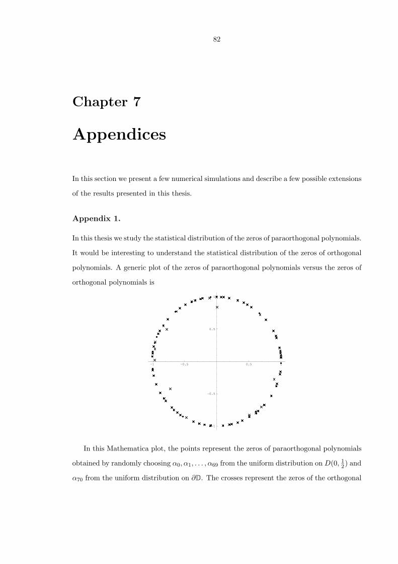
82

Chapter 7

Appendices

In this section we present a few numerical simulations and describe a few possible extensions

of the results presented in this thesis.

Appendix 1.

In this thesis we study the statistical distribution of the zeros of paraorthogonal polynomials.

It would be interesting to understand the statistical distribution of the zeros of orthogonal

polynomials. A generic plot of the zeros of paraorthogonal polynomials versus the zeros of

orthogonal polynomials is

-1 -0.5 0.5 1

-1

-0.5

0.5

1

In this Mathematica plot, the points represent the zeros of paraorthogonal polynomials

obtained by randomly choosing α0, α1, . . . , α69 from the uniform distribution on D(0, 12) and

α70 from the uniform distribution on ∂D. The crosses represent the zeros of the orthogonal

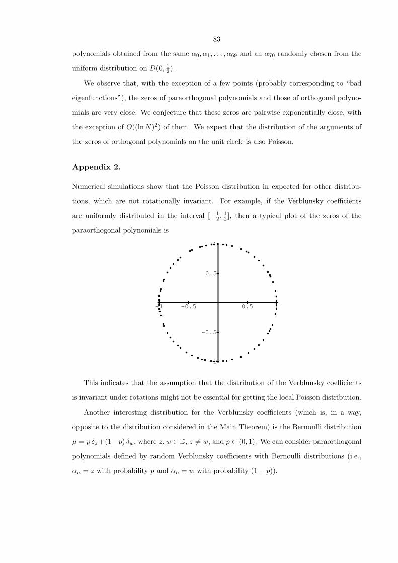
83

polynomials obtained from the same α0, α1, . . . , α69 and an α70 randomly chosen from the

uniform distribution on D(0, 12).

We observe that, with the exception of a few points (probably corresponding to “bad

eigenfunctions”), the zeros of paraorthogonal polynomials and those of orthogonal polyno-

mials are very close. We conjecture that these zeros are pairwise exponentially close, with

the exception of O((lnN)2) of them. We expect that the distribution of the arguments of

the zeros of orthogonal polynomials on the unit circle is also Poisson.

Appendix 2.

Numerical simulations show that the Poisson distribution in expected for other distribu-

tions, which are not rotationally invariant. For example, if the Verblunsky coefficients

are uniformly distributed in the interval [−12 , 1

2 ], then a typical plot of the zeros of the

paraorthogonal polynomials is

0.5 1-0.5-1

0.5

1

-0.5

-1

This indicates that the assumption that the distribution of the Verblunsky coefficients

is invariant under rotations might not be essential for getting the local Poisson distribution.

Another interesting distribution for the Verblunsky coefficients (which is, in a way,

opposite to the distribution considered in the Main Theorem) is the Bernoulli distribution

µ = p δz +(1−p) δw, where z, w ∈ D, z 6= w, and p ∈ (0, 1). We can consider paraorthogonal

polynomials defined by random Verblunsky coefficients with Bernoulli distributions (i.e.,

αn = z with probability p and αn = w with probability (1− p)).

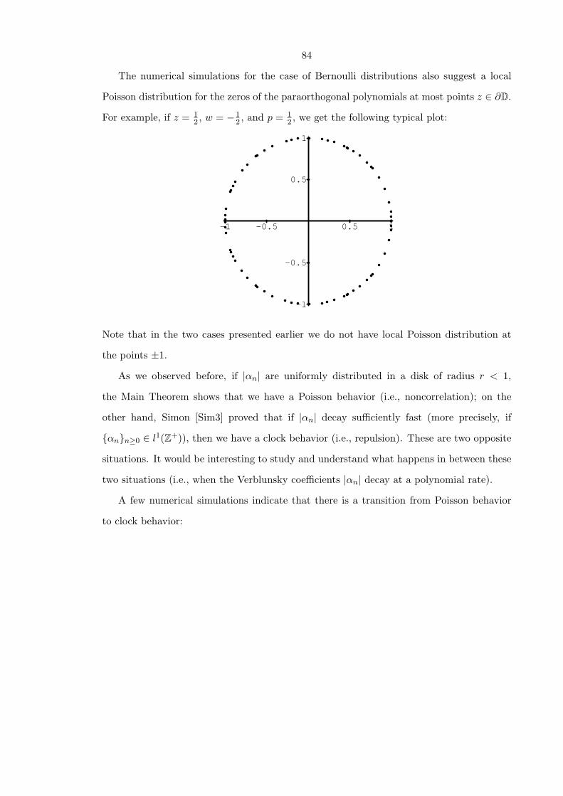
84

The numerical simulations for the case of Bernoulli distributions also suggest a local

Poisson distribution for the zeros of the paraorthogonal polynomials at most points z ∈ ∂D.

For example, if z = 12 , w = −1

2 , and p = 12 , we get the following typical plot:

0.5 1-0.5-1

0.5

1

-0.5

-1

Note that in the two cases presented earlier we do not have local Poisson distribution at

the points ±1.

As we observed before, if |αn| are uniformly distributed in a disk of radius r < 1,

the Main Theorem shows that we have a Poisson behavior (i.e., noncorrelation); on the

other hand, Simon [Sim3] proved that if |αn| decay sufficiently fast (more precisely, if

αnn≥0 ∈ l1(Z+)), then we have a clock behavior (i.e., repulsion). These are two opposite

situations. It would be interesting to study and understand what happens in between these

two situations (i.e., when the Verblunsky coefficients |αn| decay at a polynomial rate).

A few numerical simulations indicate that there is a transition from Poisson behavior

to clock behavior:

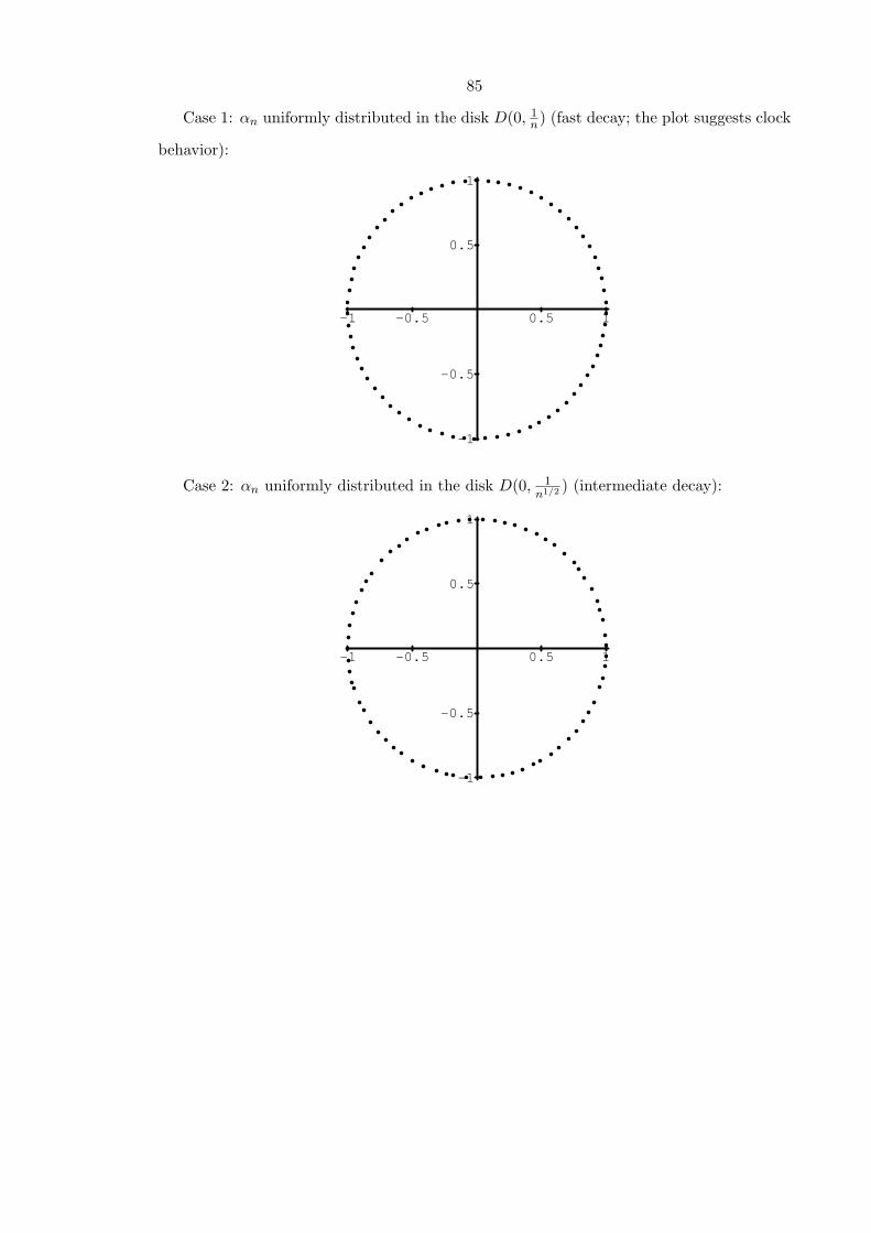
85

Case 1: αn uniformly distributed in the disk D(0, 1n) (fast decay; the plot suggests clock

behavior):

0.5 1-0.5-1

0.5

1

-0.5

-1

Case 2: αn uniformly distributed in the disk D(0, 1n1/2 ) (intermediate decay):

0.5 1-0.5-1

0.5

1

-0.5

-1

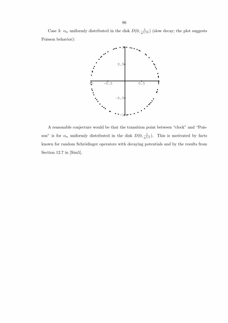
86

Case 3: αn uniformly distributed in the disk D(0, 1n1/10 ) (slow decay; the plot suggests

Poisson behavior):

0.5 1-0.5-1

0.5

1

-0.5

-1

A reasonable conjecture would be that the transition point between “clock” and “Pois-

son” is for αn uniformly distributed in the disk D(0, 1n1/2 ). This is motivated by facts

known for random Schrodinger operators with decaying potentials and by the results from

Section 12.7 in [Sim5].

87

Bibliography

[Aiz1] Michael Aizenman, personal communication.

[Aiz2] , Localization at weak disorder: some elementary bounds, Rev. Math. Phys.

6 (1994), no. 5A, 1163–1182, special issue dedicated to Elliott H. Lieb.

[AM] Michael Aizenman and Stanislav Molchanov, Localization at large disorder and

at extreme energies: an elementary derivation, Comm. Math. Phys. 157 (1993),

no. 2, 245–278.

[ASFH] Michael Aizenman, Jeffrey H. Schenker, Roland M. Friedrich, and Dirk Hundert-

mark, Finite-volume fractional-moment criteria for Anderson localization, Comm.

Math. Phys. 224 (2001), no. 1, 219–253, Dedicated to Joel L. Lebowitz.

[AlVi] M. Pilar Alfaro and Luis Vigil, Solution of a problem of P. Turan on zeros of

orthogonal polynomials on the unit circle, J. Approx. Theory 53 (1988), no. 2,

195–197.

[And] Philip W. Anderson, Absence of diffusion in certain random lattices., Phys. Rev.

109 (1958), 1492–1505.

[BHJ] Olivier Bourget, James S. Howland, and Alain Joye, Spectral analysis of unitary

band matrices, Comm. Math. Phys. 234 (2003), no. 2, 191–227.

[CMV] M. J. Cantero, L. Moral, and L. Velazquez, Five-diagonal matrices and zeros of

orthogonal polynomials on the unit circle, Linear Algebra Appl. 362 (2003), 29–56.

88

[CKM] Rene Carmona, Abel Klein, and Fabio Martinelli, Anderson localization for

Bernoulli and other singular potentials, Comm. Math. Phys. 108 (1987), no. 1,

41–66.

[CL] Rene Carmona and Jean Lacroix, Spectral theory of random Schrodinger operators,

Probability and its Applications, Birkhauser Boston Inc., Boston, MA, 1990.

[CFKS] H. L. Cycon, R. G. Froese, W. Kirsch, and B. Simon, Schrodinger operators with

application to quantum mechanics and global geometry, study ed., Texts and Mono-

graphs in Physics, Springer-Verlag, Berlin, 1987.

[DVJ88] D. J. Daley and D. Vere-Jones, An introduction to the theory of point processes,

Springer Series in Statistics, Springer-Verlag, New York, 1988.

[DVJ03] , An introduction to the theory of point processes. Vol. I, second ed., Prob-

ability and its Applications (New York), Springer-Verlag, New York, 2003.

[dRJLS] R. del Rio, S. Jitomirskaya, Y. Last, and B. Simon, Operators with singular contin-

uous spectrum. IV. Hausdorff dimensions, rank one perturbations, and localization,

J. Anal. Math. 69 (1996), 153–200.

[Dur] Peter L. Duren, Theory of Hp spaces, Pure and Applied Mathematics, Vol. 38,

Academic Press, New York, 1970.

[FS] Jurg Frohlich and Thomas Spencer, Absence of diffusion in the Anderson tight

binding model for large disorder or low energy, Comm. Math. Phys. 88 (1983),

no. 2, 151–184.

[Ger] L. Y. Geronimus, Orthogonal polynomials: Estimates, asymptotic formulas, and

series of polynomials orthogonal on the unit circle and on an interval, Authorized

translation from the Russian, Consultants Bureau, New York, 1961.

[GMP] I. Ja. Gol′dseıd, S. A. Molcanov, and L. A. Pastur, A random homogeneous

Schrodinger operator has a pure point spectrum, Funkcional. Anal. i Prilozen. 11

(1977), no. 1, 1–10, 96.

89

[Gol] Leonid Golinskii, Quadrature formula and zeros of para-orthogonal polynomials on

the unit circle, Acta Math. Hungar. 96 (2002), no. 3, 169–186.

[GN] Leonid Golinskii and Paul Nevai, Szego difference equations, transfer matrices and

orthogonal polynomials on the unit circle, Comm. Math. Phys. 223 (2001), no. 2,

223–259.

[JNT] William B. Jones, Olav Njastad, and W. J. Thron, Moment theory, orthogonal

polynomials, quadrature, and continued fractions associated with the unit circle,

Bull. London Math. Soc. 21 (1989), no. 2, 113–152.

[Joye1] Alain Joye, Density of states and Thouless formula for random unitary band ma-

trices, Ann. Henri Poincare 5 (2004), no. 2, 347–379.

[Joye2] , Fractional moment estimates for random unitary operators, preprint

(2004).

[Kho] Andrei Khodakovsky, Inverse spectral problem with partial information on the po-

tential, Ph.D. Thesis, Caltech (1999).

[Khr] Sergei Khrushchev, Schur’s algorithm, orthogonal polynomials, and convergence of

Wall’s continued fractions in L2(T), J. Approx. Theory 108 (2001), no. 2, 161–248.

[Kin] J. F. C. Kingman, Poisson processes, Oxford Studies in Probability, vol. 3, The

Clarendon Press Oxford University Press, New York, 1993, Oxford Science Publi-

cations.

[McK] H. P. McKean, Jr., Stochastic integrals, Probability and Mathematical Statistics,

No. 5, Academic Press, New York, 1969.

[Mi] Nariyuki Minami, Local fluctuation of the spectrum of a multidimensional Ander-

son tight binding model, Comm. Math. Phys. 177 (1996), no. 3, 709–725.

[Mo1] S. A. Molcanov, Structure of the eigenfunctions of one-dimensional unordered

structures, Izv. Akad. Nauk SSSR Ser. Mat. 42 (1978), no. 1, 70–103, 214.

90

[Mo2] , The local structure of the spectrum of the one-dimensional Schrodinger

operator, Comm. Math. Phys. 78 (1980/81), no. 3, 429–446.

[Pas] L. A. Pastur, Spectra of random selfadjoint operators, Uspehi Mat. Nauk 28 (1973),

no. 1(169), 3–64.

[Pok] V. L. Pokrovskij, Distribution function of distances between energy levels of an

electon in a one-dimensional random chain, Letters of GETF 4 (1966).

[Sim1] Barry Simon, Aizenman’s theorem for orthogonal polynomials on the unit circle,

to appear in Const. Approx.

[Sim2] , Spectral analysis of rank one perturbations and applications, Mathematical

Quantum Theory. II. Schrodinger Operators (Vancouver, BC, 1993), CRM Proc.

Lecture Notes, vol. 8, Amer. Math. Soc., Providence, RI, 1995, pp. 109–149.

[Sim3] , Fine structure of the zeros of orthogonal polynomials, i. a tale of two

pictures, preprint (2005).

[Sim4] , Orthogonal polynomials on the unit circle, part 1: Classical theory, AMS

Colloquium Series, American Mathematical Society, Providence, RI, 2005.

[Sim5] , Orthogonal polynomials on the unit circle, part 2: Spectral theory, AMS

Colloquium Series, American Mathematical Society, Providence, RI, 2005.

[ST] Barry Simon and Vilmos Totik, Limits of zeros of orthogonal polynomials on the

circle, to appear in special issue of Math. Nachr. in honor of F.V. Atkinson.

[SW] Barry Simon and Thomas Wolff, Singular continuous spectrum under rank one

perturbations and localization for random Hamiltonians, Comm. Pure Appl. Math.

39 (1986), no. 1, 75–90.

[Sto] Mihai Stoiciu, The statistical distribution of the zeros of random paraorthogonal

polynomials on the unit circle, to appear in J. Approx. Theory.

[Tep] A. V. Teplyaev, The pure point spectrum of random orthogonal polynomials on the

circle, Dokl. Akad. Nauk SSSR 320 (1991), no. 1, 49–53.

91

[Tes] Gerald Teschl, Jacobi operators and completely integrable nonlinear lattices, Math-

ematical Surveys and Monographs, vol. 72, American Mathematical Society, Prov-

idence, RI, 2000.