yige thesis 0319 - texas a&m university
TRANSCRIPT

ALGORITHMS AND SOFTWARE TOOLS FOR EXTRACTING COASTA L
MORPHOLOGICAL INFORMATION FROM AIRBORNE LiDAR DATA
A Thesis
by
YIGE GAO
Submitted to the Office of Graduate Studies of Texas A&M University
in partial fulfillment of the requirements for the degree of
MASTER OF SCIENCE
May 2009
Major Subject: Geography

ALGORITHMS AND SOFTWARE TOOLS FOR EXTRACTING COASTA L
MORPHOLOGICAL INFORMATION FROM AIRBORNE LiDAR DATA
A Thesis
by
YIGE GAO
Submitted to the Office of Graduate Studies of Texas A&M University
in partial fulfillment of the requirements for the degree of
MASTER OF SCIENCE
Approved by:
Chair of Committee, Hongxing Liu Committee Members, Andrew Millington Xinyuan Ben Wu Head of Department, Douglas J. Sherman
May 2009
Major Subject: Geography

iii
ABSTRACT
Algorithms and Software Tools for Extracting Coastal Morphological Information
from Airborne LiDAR Data. (May 2009)
Yige Gao, B.S.; B.S., Peking University, Beijing, China
Chair of Advisory Committee: Dr. Hongxing Liu
With the ever increasing population and economic activities in coastal areas, coastal
hazards have become a major concern for coastal management. The fundamental
requirement of coastal planning and management is the scientific knowledge about
coastal forms and processes. This research aims at developing algorithms for
automatically extracting coastal morphological information from LiDAR data. The
primary methods developed by this research include automated algorithms for beach
profile feature extraction and change analysis, and an object-based approach for spatial
pattern analysis of coastal morphologic and volumetric change.
Automated algorithms are developed for cross-shore profile feature extraction
and change analysis. Important features of the beach profile such as dune crest, dune toe,
and beach berm crest are extracted automatically by using a scale-space approach and by
incorporating contextual information. The attributes of important feature points and
segments are derived to characterize the morphologic properties of each beach profile.
Beach profiles from different time periods can be compared for morphologic and
volumetric change analysis.

iv
An object-oriented approach for volumetric change analysis is developed to
identify and delineate individual elevation change patches as discrete objects. A set of
two-dimensional and three-dimensional attributes are derived to characterize the objects,
which includes planimetric attributes, shape attributes, surface attributes, volumetric
attributes, and summary attributes.
Both algorithms are implemented as ArcGIS extension modules to perform the
feature extraction and attribute derivation for coastal morphological change analysis. To
demonstrate the utility and effectiveness of algorithms, the cross-shore profile change
analysis method and software tool are applied to a case study area located at southern
Monterey Bay, California, and the coastal morphology change analysis method and
software tool are applied to a case study area located on Assateague Island, Maryland.
The automated algorithms facilitate the efficient beach profile feature analysis
over large geographical area and support the analysis of the spatial variations of beach
profile changes along the shoreline. The explicit object representation of elevation
change patches makes it easy to localize erosion hot spots, to classify the elevation
changes caused by various mechanisms, and to analyze spatial pattern of morphologic
and volumetric changes.

v
DEDICATION
Dedicated to
My parents

vi
ACKNOWLEDGMENTS
I would like to express my greatest gratitude to my advisor, Dr. Hongxing Liu. Your
patient guidance and unceasing encouragement helped me to push my way along this
research journey. I could never achieve this point without your guidance both in research
and in life attitude.
Thanks to my committee members Dr. Andrew Millington and Dr. Xinyuan Ben
Wu for your insightful advice and valuable comments on this research.
Thanks to Dr. Jinfeng Wang and all my colleagues in Lab201 back in China – I
enjoyed all the time we spend together. Without your help and encouragement, I
wouldn’t have had the opportunity to be in this land of America.
Thanks to Dean, Zichuan, and everyone in water resources team in ESRI — I
never expected such a wonderful internship and such a friendly working environment.
Thanks for all your patient guidance in helping me to learn about hydrological and
hydraulic modeling.
Thanks to Lei Wang, Sheng-jung Tang, and Zengwang Xu for all the wonderful
time we spent together and your endless help and encouragement after graduation.
Thanks to my good friends in Texas A&M: Bailiang Li, Li Li, Haibin Su, Bing-Sheng
Wu, Rahul, Luti, Shinichi, Alehe, Iliyana, and Cara for your big-hearted support and all
the fun time we shared during the past two years. Thanks to Songgang Gu and Zheng
Cheng – I understand your choice and hope you have a bright future.

vii
I also would like to share my joy and happiness with my dear friends Qian Di,
Dong Han, Bin Leng, Xin Jin, and Shuangshi Yin in China, for their consistent
understanding and encouragement during all these years, no matter where I am.
Last, but most important, I want to thank my parents for being such a wonderful
example, teaching me to be a trustworthy person, be true to friends, be responsible for
work, and always be positive towards life. Thanks for your endless love and support.

viii
TABLE OF CONTENTS Page
ABSTRACT..................................................................................................................... iii DEDICATION ...................................................................................................................v ACKNOWLEDGMENTS.................................................................................................vi TABLE OF CONTENTS............................................................................................... viii LIST OF FIGURES............................................................................................................x LIST OF TABLES ......................................................................................................... xiii 1 INTRODUCTION......................................................................................................1
1.1 Background ....................................................................................................1 1.2 Objectives.......................................................................................................3 1.3 Methodology ..................................................................................................4
1.3.1 Automated feature extraction and change analysis for cross-shore profiles.............................................................................4 1.3.2 Object-based morphological and volumetric change analysis ...........4
1.4 Organization of the thesis...............................................................................5 2 LITERATURE REVIEW...........................................................................................7
2.1 Coastal topography mapping techniques........................................................7 2.2 Methods and software for beach profile feature extraction and change analysis...............................................................................................9 2.3 Pixel-based morphological change analysis.................................................16
3 LiDAR DATA PREPROCESSING .........................................................................22
3.1 Airborne LiDAR remote sensing system .....................................................22 3.2 Basic LiDAR products .................................................................................23 3.3 LiDAR data preprocessing ...........................................................................25
4 MORPHOLOGIC ATTRIBUTES EXTRACTION AND CHANGE ANALYSIS BASED ON BEACH PROFILES............................................................................29
4.1 Mathematical principles for extracting morphological features from beach profiles.......................................................................................29

ix
Page
4.1.1 Typical beach profile and definition of morphological features......29 4.1.2 Morphological feature extraction from an ideal beach profile.........33
4.2 Morphological feature extraction from natural beach profiles.....................37 4.2.1 Scale-space approach to feature extraction from beach profiles......39 4.2.2 Incorporate contextual information for feature extraction
of beach profile.................................................................................45 4.2.3 Procedures for deriving morphologic attributes for beach
profiles along the shoreline ..............................................................53 4.2.4 Derivation of attributes for characterizing beach profiles
and profile changes...........................................................................55 4.3 ArcGIS extension module for beach profile analysis...................................56
5 OBJECT-BASED METHOD FOR MORPHOLOGICAL AND
VOLUMETRIC CHANGE ANALYSIS .................................................................63
5.1 Identification and delineation of elevation change objects ..........................63 5.2 Attribute derivation for characterizing erosion and deposition objects .......67
5.2.1 Planimetric attributes .......................................................................68 5.2.2 Shape attributes ................................................................................69 5.2.3 Surface attributes..............................................................................77 5.2.4 Volumetric attributes........................................................................79 5.2.5 Summary statistical attributes ..........................................................79
5.3 ArcGIS extension module for volumetric change analysis ..........................82 6 CASE STUDIES ......................................................................................................85
6.1 A case study for beach profile feature extraction and change analysis........85 6.1.1 LiDAR data preprocessing...............................................................86 6.1.2 Beach profile feature extraction and change analysis ......................89
6.2 A case study for object-based morphological and volumetric change analysis ........................................................................103 6.2.1 LiDAR data preprocessing.............................................................104 6.2.2 Morphological and volumetric change analysis.............................105
7 CONCLUSIONS....................................................................................................114 REFERENCES...............................................................................................................118 VITA ..............................................................................................................................122

x
LIST OF FIGURES
Page Figure 4.1 Illustration of morphological features of the coastal zone..........................31
Figure 4.2 A simplified hypothetic beach profile ........................................................35
Figure 4.3 Slope and curvature derived for a simplified hypothetic beach profile ......36
Figure 4.4 A natural beach profile ...............................................................................38
Figure 4.5 Slope and curvature derived for a natural beach profile .............................38
Figure 4.6 Gaussian distributions with different standard deviations..........................40
Figure 4.7 Feature extraction of beach profile at smooth scale σ =1 ..........................42
Figure 4.8 Feature extraction of beach profile at smooth scale σ =2 ...........................43
Figure 4.9 Feature extraction of beach profile at smoothing scale σ =4 .....................44
Figure 4.10 Mistakenly identified dune crest (smoothing scale σ =2) ..........................45
Figure 4.11 Example of dune crest identification based on information from individual beach profile . ....................................................................46
Figure 4.12 Adjustment of dune crest location using compatibility values ...................51
Figure 4.13 Example of dune crests identification.........................................................52
Figure 4.14 ArcGIS extension module – Profile Analyst ..............................................57
Figure 5.1 Identification of elevation change objects ..................................................64
Figure 5.2 A minimum bounding rectangle and its parameters ...................................75
Figure 5.3 Steps of fitting minimum bounding rectangle ............................................75
Figure 5.4 Best-fit ellipse and its parameters ...............................................................76
Figure 5.5 ArcGIS extension module - Coastal Volumetric Analyst...........................83
Figure 6.1 The geographical settings of Marina, southern Monterey Bay, California..86

xi
Page
Figure 6.2 Stillwell Hall, Marina, CA.. .........................................................................87
Figure 6.3 LiDAR DEMs and the elevation difference grid. .........................................88
Figure 6.4 Monthly mean high water level relative to NAVD88 during 1997- 1998 winter..............................................................................90
Figure 6.5 Beach transects generated along the shoreline .............................................90
Figure 6.6 Beach feature extraction from spring 1998 LiDAR data. .............................91
Figure 6.7 Comparison between the feature points identified with and without using contextual information ...........................................92
Figure 6.8 Beach feature extraction from fall 1997 and spring 1998 LiDAR data........94
Figure 6.9 Beach feature extraction from fall 1997 and spring 1998 LiDAR data........95
Figure 6.10 Profiles across seawall (fall 1997) ...............................................................97
Figure 6.11 Variations of bluff crest elevation, bluff toe elevation, and bluff height along shoreline in the area nearby seawall (fall 1997)................................98
Figure 6.12 Example of high bluff and low bluff ...........................................................99
Figure 6.13 Elevation change for Profile 130 (across Stillwell Hall) ...........................100
Figure 6.14 Change of bluff crest and bluff toe’s distance to the shoreline (year 1998 – year 1997) ............................................................................101
Figure 6.15 Bluff crest and toe recession next to the seawall . .....................................101
Figure 6.16 Change of bluff crest and bluff toe’s elevation (year 1998 – year 1997) ..102
Figure 6.17 Change in bluff and beach volume (year 1998 – year 1997).....................103
Figure 6.18 The geographical settings of Whittington Point of Assateague Island, Maryland ....................................................................104
Figure 6.19 LiDAR DEMs and the elevation difference grid ......................................106
Figure 6.20 Negative change and positive change objects............................................108
Figure 6.21 Erosion and deposition objects after smoothing ........................................108

xii
Page
Figure 6.22 Erosion and deposition objects overlaid on the hill-shaded relief images.109
Figure 6.23 Fitted rectangles and ellipse for erosion and deposition objects ...............111

xiii
LIST OF TABLES
Page Table 4.1 Compatibility values calculated based on contextual information ................51
Table 5.1 Definitions of planimetric attributes ..............................................................69
Table 5.2 Definitions of shape attributes ......................................................................71
Table 5.3 Definitions of surface attributes ....................................................................78
Table 5.4 Definitions of volumetric attributes ..............................................................80
Table 5.5 Definitions of summary statistical attributes.................................................81
Table 6.1 Beach profile attributes derived for (a) year 1997; (b) year 1998; and (c) changes...............................................95
Table 6.2 Derived attributes values for erosion and deposition objects......................110

1
1 INTRODUCTION
1.1 Background
Coastal areas sustain a wealth of natural resources and economic activities. More than
half of the world’s population currently lives within 60 km of the coastline, and the
coastal concentration of population is expected to increase dramatically in the future
(CCSR, 2006). In the U.S., it is estimated approximately 53% percent of the nation’s
population lived in coastal counties in 2003, which is expected to increase by 12 million
by 2015 (Crossett et al., 2004). With the ever increasing population and economic
activities in coastal areas, coastal hazards have become a major concern for coastal
management. The fundamental requirement of coastal management and planning is the
scientific knowledge about coastal morphology and processes. The information about the
coastal morphology change could facilitate decision-makers to better understand coastal
process, to assess and predict the impacts of coastal hazards, and to formulate better
management decisions regarding sustainable coastal developments.
Traditionally, coastal mapping has been based on ground surveys of transects
perpendicular and parallel to the shoreline. In most cases it is time-consuming and labor-
intensive. Transects are usually widely spaced due to time and cost restrictions. In recent
years, airborne LiDAR remote sensing technology has been widely used in surveying,
mapping and monitoring coastal environmental conditions and changes. LiDAR
technique provides a much more cost-effective and efficient means of collecting
topographic information, which allows a detailed analysis of micro-geomorphology of
______________ This thesis follows the style of Annals of the Association of American Geographers.

2
the coastal area over a broad region (White and Wang, 2003; Brock et al., 2004; Zhang
et al., 2005; Finkl et al., 2005). The technological advancements present both
opportunities and challenges. One of the major challenges brought by the LiDAR
technology is to develop methods to fully explore high resolution LiDAR data for
information and knowledge extraction.
Cross-shore profile change analysis provides an important dimension in
understanding morphological and volumetric changes in coastal area. Beach profiles can
be extracted from the LiDAR surveys at a much higher resolution than those from
traditional ground-based surveys for detailed change analysis (Brock et al., 2004). The
available analytical techniques for beach profile change analysis include the comparison
of successive surveys in terms of beach height, width, gradient, and shape, as well as the
beach profile areas and volumes (Cooper et al., 2000). However, previous studies are
primarily based on the visual interpretation of profiles and simple statistical analysis for
extracting morphologic features of beach profiles such as dune crests and toes (Elko et
al., 2002; Judge et al., 2003; Zhang et al., 2005; Gares et al., 2006; Robertson et al.,
2007). This research intends to develop automated algorithms for extracting cross-shore
profiles, identifying critical points, and calculating important cross-shore morphological
properties from LiDAR data.
Information about spatial patterns of erosion and deposition and corresponding
volumetric changes of the coastal zone are important for coastal hazard evaluation and
coastal management. Previously, a cell-by-cell differencing method was commonly used
for the volumetric change analysis based on LiDAR surveys (Woolard and Colby, 2002;

3
White and Wang, 2003; Shrestha et al., 2005; Zhang et al., 2005; Gares et al., 2006). The
volume change is evaluated on a cell-by-cell basis by subtracting the LiDAR DEM
acquired at an earlier time from the LiDAR DEM acquired at a later time. However,
such an approach suffers from the difficulty in deriving localized information to analyze
spatial patterns of morphologic and volumetric changes. It is also difficult to recognize
elevation changes induced by factors other than erosion and deposition. In addition, it is
not convenient with the cell-by-cell differencing method to associate the volumetric
change information with other data for interpreting the causes and impacts of volumetric
changes. This research aims to develop an object-based approach to morphologic and
volumetric change analysis, which explicitly identifies each individual erosion and
deposition patch as discrete object, and derive a set of spatial and volumetric attributes to
characterize each object.
1.2 Objectives
The general goal of this research is to develop algorithms for automatically extracting
coastal morphological change information. Specific objectives include:
• Develop automated algorithms for beach profile feature extraction and change
analysis
• Develop an object-based approach for coastal morphological and volumetric
change analysis
• Implement software tools for coastal morphological change analysis
• Test and validate coastal morphological change analysis methods for case study
areas

4
1.3 Methodology
1.3.1 Automated feature extraction and change analysis for cross-shore profiles
This research will develop numerical algorithms for cross-shore profile feature
extraction and change analysis based on repeat LiDAR data. Beach profiles
perpendicular to the shoreline will be automatically generated at a given interval. The
Gaussian filter will be applied to smooth the beach profiles. Slope and curvature values
will be calculated for different sections of the beach profile. The dune crest and toe, as
well as the beach berm crest will be identified based on the slope and curvature values.
The attributes such as slopes for dune face and beach, as well as the heights and
horizontal positions for dune crest and berm crest will be derived to characterize the
morphologic properties of beach profile. To refine and improve the computation results
from individual profiles, which are usually noisy, the contextual information of adjacent
profiles are incorporated in the computation. The beach profiles from successive LiDAR
surveys are compared for morphological and volumetric change analysis. This
automated profile analysis method will be implemented as ArcGIS extension module to
perform the feature extraction and attribute derivation from LiDAR beach profiles.
1.3.2 Object-based morphological and volumetric change analysis
This research will develop an object-based approach for volumetric change analysis
using repeat LiDAR data. This approach automatically identifies and delineates
individual erosion and deposition patches as discrete objects. These erosion and
deposition objects, instead of individual cells in the elevation differencing grid, are used
as basic spatial units for volumetric analysis. A set of two-dimensional and three-

5
dimensional attributes will be derived to characterize and quantify erosion and
deposition objects, which includes planimetric attributes, shape attributes, volumetric
attributes, and summary statistical attributes. The explicit object representation of
erosion and deposition patches makes it easy to localize hot spots, to analyze spatial
pattern of morphologic and volumetric changes, to discriminate the erosion and
deposition caused by different factors, and to incorporate other GIS data to explore the
causes and impacts of the changes. This method will be implemented as an ArcGIS
extension module to perform the object identification and attribute derivation.
1.4 Organization of the thesis
This thesis consists of six sections. The present section introduces the research
background, objectives, and methodology.
Section 2 reviews the existing coastal topography mapping techniques, the pixel-
based method for coastal morphological and volumetric analysis, and the existing
methods and softwares for feature extraction and change analysis of beach profile.
Section 3 introduces the airborne LiDAR remote sensing system and basic data
products, and discusses the workflow for LiDAR data preprocessing.
Section 4 presents the automated method for beach profile feature extraction and
attribute derivation, as well as the approach for profile change analysis based on
sequential LiDAR data.
Section 5 presents the object-based method, which includes the identification and
delineation of erosion and deposition objects, as well as the derivation of attributes for
characterizing these objects.

6
Section 6 applies the change analysis method described in Section 4 and Section
5 to case study areas.
The last section summarizes the research findings and discusses the future
research directions.

7
2 LITERATURE REVIEW
This section reviews the coastal mapping techniques and discusses the comparative
advantages of airborne LiDAR technology. The pixel-based approach for coastal
morphological and volumetric analysis is introduced and its limitations are discussed. In
addition, the visual interpretation and conventional methods for feature extraction from
beach profiles, and the existing change analysis methods and software tools are reviewed
and summarized.
2.1 Coastal topography mapping techniques
The coastal topography measurements are required by many studies such as coastal
flood forecasting, coastal defence structure design against flooding and erosion, coastal
environmental management, and environment impact assessment for economic
exploitation (Mason et al., 2000). Traditionally, coastal topography mapping is based on
methods such as ground survey and photogrammetry. In recent years, the development
of airborne LiDAR remote sensing technology provides a much more cost-effective and
efficient method to acquire elevation information in coastal area.
Ground surveys for coastal areas are usually based on transects perpendicular
and/or parallel to the shoreline. The elevation measurements along transects are acquired
by using instruments such as engineer’s levels, total stations, or Global Positioning
System (GPS) instruments (Cooper et al., 2000). The ground surveys can obtain highly
accurate elevation measurements along transects and are repeatable at different time
periods, which is necessary for change analysis. The topography of the near-shore zones

8
can be monitored by extending transects below water surface. However, in most cases
this method is time-consuming and labor-intensive. When a large area needs to be
covered, it means either a significant increase in cost, time, and labor to measure
sufficient number of transects to represent the topography, or a sparse sampling rate,
which may not be representative of the topography in details, and thus compromise the
objective of study. In addition, the ground surveys are always constrained by the tidal
and weather conditions, as well as the safety and accessibility of the survey area.
The photogrammetric approach extracts the elevation information from
stereoscopic aerial photography. By acquiring aerial photographs from different vantage
view points of the landscape, the elevation measurements of the terrain surface in the
overlapping areas of multiple photographs could be calculated based on stereoscopic
parallax, which is the change of its viewing position from one photograph to the next
relative to its background. The resulting digital elevation model (DEM) derived by
photogrammetric approach could be at various scales (Jensen, 2007). This method could
derive highly accurate elevation measurements and the data collection is repeatable.
Depending on the required flying scale and level of accuracy, the cost could vary for
both flying and image interpretation. Compared to ground survey methods, stereoscopic
aerial photography could cover a large area with much better spatial resolution. However,
the difficulty in identifying match points on featureless areas like beaches and dunes has
seriously hindered photogrammetry application in coastal areas (Mason et al., 2000).
The elevation extraction process from photogrammetry is relatively costly and time
consuming. It cannot obtain the elevation measurements under water and cannot be used

9
for topography mapping in the near-shore zone. The flying missions are seriously
constrained by weather and lighting conditions.
The airborne LiDAR technology is based on accurate measurements of the laser
pulse travel time from the transmitter to the target and back to the receiver. The laser
scanner sends thousands of laser beams per second to the ground. Using the sensor
position derived from differential Global Positioning System (GPS) and the sensor
orientation derived from Inertial Measurement Unit (IMU), the laser range
measurements can be converted to highly accurate elevation values. For coastal
topography mapping, most LiDAR systems use near-infrared laser light in the region
from 1045 to 1065 nm, which may also be used for mapping topography in the near-
shore zone depending on the water clarity. The LiDAR techniques could achieve high
vertical accuracy of approximately 15 cm and horizontal accuracy of less than 1m
(NOAA, 2008). Compared to ground surveys and photogrammetric data, LiDAR data
can be collected at night if necessary because it is an active system and does not rely on
the solar illumination. The requirements of LiDAR system for weather and lighting
conditions are not as strict as that of aerial photography, and the data processing
procedure is much simpler and more efficient. Overall, it provides a cost-effective and
efficient way to collect detailed elevation measurements over a large coastal region.
2.2 Methods and software for beach profile feature extraction and change
analysis
Beach profile surveying is a long-established and widely used technique for coastal
monitoring. Cooper et al. (2000) provided a summary of the key elements of the beach

10
profile measurement, theory and analysis. They classified the beach profile change
analysis methods into two categories: temporal analytical methods that assesses changes
along one particular beach profile with respect to time, and spatial analytical methods
that assesses variations between different profiles. The temporal analytical method can
be used to identify the shore-term variation and long-term trends at a specific location
and the spatial analytical method can be used to determine the spatial pattern of beach
profile changes along the coastline. They summarized the available analytical techniques
for comparison of successive surveys along a beach profile. The profiles can be
compared in terms of beach level and width, which are regarded as the standard of
natural coastal defence. Also, the profiles can be compared in terms of beach gradient to
understand the trends for beach steepening or flattening, and in terms of beach profile
areas and volumes to evaluate the ‘health’ of beach.
Most of the previous studies used visual interpretation approach to extract
morphological features from beach profiles. In recent years, some efforts have been
made to develop numerical methods to identify and extract features from beach profiles.
Brock et al. (2004) developed LiDAR metrics for barrier island elevation profiles to
analyze morphological changes. For each LiDAR-based cross-shore profile, they
determined the ocean shoreline point, bay shoreline point, and the volume balanceline
point. The LiDAR change metrics were developed to describe the ocean shoreline
displacement, bay shoreline displacement, volume balanceline displacement, and the
slice volume change. A morphodynamic classification was presented based on LiDAR
change metrics. To support a storm impact scaling model for analyzing dune

11
vulnerability to storm-induced erosion (Sallenger, 2000), a semi-automated algorithm
was developed for extracting dune crest and dune toe from LiDAR data (Elko et al.,
2002). First, the approximate locations of the dune crest and toe line had to be digitized
manually. The dune crest line or berm crest line were visually recognized and manually
digitized from the aspect image as the transition line from seaward-sloping to landward-
sloping regions. The dune base line was delineated from the slope image as the transition
line between the flat beach and the steep dune face. The authors pointed out that the
dune base delineation were generally more difficult because there might not be distinct
break between dune face and beach. Then, a searching algorithm was utilized to
automatically determine the actual heights of dune crests and toes within a buffer around
the digitized line. To obtain the dune crest height, a neighborhood function was applied
to select the pixel with maximum elevation value within the 7 m wide buffer around the
digitized dune crest line. To avoid small perturbations with rapidly changing slopes near
the dune toe, a smaller buffer area of 3-m wide was created around the digitized dune toe
line, and a neighborhood function was applied to select the pixel with maximum value of
the second derivative of elevation as the dune toe pixel. Stockdon et al. (2007) adopted
this method to identify the pre-storm elevation of the dune crest and toe, which were
used in conjunction with expected water levels to predict the spatially-varying storm-
impact regime.
A quantitative method has been developed by USGS Center for Costal and
Regional Marine Studies to automatically extract the location and elevation of the “first
line of defense”, which could be the dune crest/ beach berm, or the top of the coastal

12
defense structures (USGS, 2008). First, this method smoothes the profile extracted from
LiDAR data so as to eliminate the small variations in elevation measurements. Second,
elevation peaks are identified based on the changes in direction of slope, and the “first
line of defense” is identified as the first elevation peak landward of the shoreline on the
profiles.
Coastal morphology analysis software such as the Beach Morphology Analysis
Package (BMAP) (Wise, 1995) and Regional Morphology Analysis Package (RMAP)
(Batten and Kraus, 2005) have been widely used by coastal community. Both of them
are part of the Coastal Engineering Design and Analysis System (CEDAS), which is an
interactive coastal design and analysis software developed by the U.S. Army Engineer
Waterways Experiment Station (Veri-Tech, 2006). CEDAS includes four modules: the
General module contains the numerical methods for coastal and hydraulic engineering
applications, the Inlet module contains the models for tidal inlet analysis, the Beach
module contains the tools for beach process analysis, and the Surface-water Modeling
System is a graphical user environment for accessing a multi-dimensional hydrodynamic
model ADCIRC and a variety of multi-dimensional surface water modeling programs.
Beach Morphology Analysis Package (BMAP) is an integrated set of interactive
tools developed to support the analysis of the morphologic and dynamic properties of
beach profiles. It is dynamically linked with SBEACH (Storm-induced BEAch CHange),
which simulates cross-shore beach, berm, and dune erosion. The capabilities of BMAP
in analyzing static properties of profiles include (Wise, 1995): plotting individual or
multiple beach profile surveys, averaging multiple profile surveys within a given spatial

13
range, generating best-fit equilibrium profile for a single grain size, calculating profile
volume with respect to specified reference elevation along the profile, generating
synthetic profiles, as well as calculating bar properties such as minimum depth and
location, maximum height and location, volume, and the center of mass. As for the
beach profile change analysis, the capabilities of BMAP include: determining cut and fill
areas with respect to cross-shore distance, calculating volume change and elevation
change between two successive profiles, and calculating cross-shore sand transport rate
by integrating the equation for conservation of sand.
The Regional Morphology Analysis Package (RMAP), which is evolved from
BMAP, also belongs to the Beach module of CEDAS (Batten and Kraus, 2005). While
BMAP is limited in distance-elevation space, RMAP can manipulate, visualize, and
analyze shoreline data and beach profiles spatially. Particularly, the shoreline positions
and beach profiles can be projected and displayed on aerial photographs or maps. Data
can be examined in both beach profile view and map view, which facilitates the quality
control, visualization, and analysis process. RMAP has the capability to import beach
profiles, shorelines, and baselines data from ASCII files, BMAP files, and spreadsheets.
It can also import shorelines and baselines from ESRI Shapefiles. Since the distance and
elevation values of each point along the profile are required to analyze the beach
morphology, RMAP can calculate the distance from the known profile origin
coordinates for each point along the transect using its XY coordinates. In order to locate
points along the profile on the map, RMAP can also calculate the XY coordinates for
each point using its distance and elevation values.

14
The Beach Profile Analysis Toolbox (BPAT) is a software for archiving, viewing,
and analyzing beach profile information, which has been developed by the National
Institute of Water and Atmospheric Research (NIWA) and Katoa Software in New
Zealand. It includes an Archive mode and an Analysis mode. The Archive mode is used
to view existing data and enter new data. The surveys within a study area are arranged
hierarchically by regions, cross-sections, and the benchmarks. The Analysis mode is
used to analyze beach profiles, which supports plotting groups of surveys for a specified
cross section, aligning surveys at a given elevation or on the basis of common marker,
calculating the slope and volume for each horizontal slice for selected single survey by
choosing a starting elevation and an elevation increment, calculating the slope and
volume for each vertical slice for selected single survey by choosing a starting offset and
an offset increment, and calculating cut/fill volume of surveys taken at different times.
The Shoreline and Nearshore Data System (SANDS) is a coastal data capture,
monitoring and analysis software developed by Halcrow Group Ltd, UK (Halcrow,
2008). It is capable of importing beach profile survey data as well as time series wave,
wind or tide level records. In SANDS, beach profile surveys can be analyzed using
different methods. The standard beach profile analysis method include the “chainage”
method, which works by dividing profile into vertical sections and calculating the beach
level at each section, and the “level” method which looks at the horizontal strips of
profile. In addition, SANDS can calculate the cross-sectional areas and volumes in
relation to a ‘master profile’, which is a rock or clay bed layer under the beach material.
As for volumetric analysis, SANDS enables the ability to group specific beach profile

15
locations to form a “Coastal Process Unit” and calculate volumes of beach materials for
these units. In SANDS, maps can be imported as backdrop for reference and may also
have data attached to it. However, SANDS is not a GIS system and the map data needs
to be prepared using other GIS software.
The visual interpretation of beach profile extracted from LiDAR data provides an
intuitive way to analyze the beach morphological change. Despite the recent
development of semi-automated algorithms, more efficient and accurate methods are
needed for automatically extracting beach profiles, identifying critical points, calculating
important morphological properties, and extracting profile change information from
LiDAR data. The available software provide useful tools for beach profile data
management and analysis. However, they failed to take advantage of dense datasets
collected by LiDAR systems to analyze data spatially. First, the elevation measurements
along beach profiles can only be imported from existing text files and be displayed on
the background map, but cannot be directly extracted from LiDAR DEM. Second, the
important features such as dune crest and toe, and berm crest are identified based on
visual interpretation, which restricts a quantitative change analysis of profiles for a large
geographic area. Third, although the beach profiles could be displayed spatially on the
background map, it is still difficult to visualize and analyze the spatial variations of
changes between different profiles along the shoreline. Fourth, the beach profile
information is not fully integrated with geographic information system and cannot be
edited and visualized interactively.

16
To address the above research gaps, this research presents automated algorithms
for cross-shore profile feature extraction and change analysis. Important features of the
beach profile are identified automatically based on the calculation of slope and curvature
values. The attributes such as slopes for dune face and beach, as well as the heights and
horizontal positions for dune crest and berm crest are derived to characterize the
morphologic properties of each beach profile. The quantitative identification and
attributes derivation of profile features enables more efficient coastal morphology
analysis for a large geographic area. The spatial patterns of the beach profile features and
the related changes can be visualized and analyzed along the shoreline. The object
representation of profile features could also facilitate the analysis in conjunction with
other GIS data for exploring the causes and impacts of the morphological and volumetric
changes at the cross-shore dimension.
2.3 Pixel-based morphological change analysis
Traditionally, the pixel-based differencing method was commonly used for the
morphological and volumetric change analysis based on LiDAR surveys (Meredith et al.,
1999; Woolard and Colby 2002; White and Wang 2003; Zhang et al. 2005; Gares et al.
2006). The volumetric change is evaluated by subtracting the LiDAR DEM acquired at
an earlier time from the LiDAR DEM acquired at a later time. A negative elevation
difference of a cell indicates that the surface material was eroded during the time span
between two LiDAR surveys. A positive elevation difference indicates that the sediment
accretion occurred, and a zero value indicates that there was no net change.

17
For the traditional pixel-based approach, the spatial pattern of morphological
changes can be visually interpreted. However, it cannot explicitly represent individual
elevation change patches and extract information for each patch. For early coastal
change studies based on LiDAR data, the morphological change information was usually
only derived for the entire study area. In recent years, some efforts have been made to
localize the change information. Woolard and Colby (2002) evaluated dune volume
changes for two small study sites (100 x 200 m) located in Cape Hatteras National
Seashore, North Carolina for a 1-year period of time using sequential LiDAR DEM. The
volumetric change measurements were compared at spatial resolutions ranging from 1 x
1 to 20 x 20 m to decide which resolution provides the most reliable representation of
coastal dunes and the most accurate change measurements. In their study, only the total
volume of erosion, deposition, and net change results were calculated and compared.
Meredith et al. (1999) assessed hurricane-induced beach erosion between fall
1997 and fall 1998 along the entire North Carolina coastline (approximately over 500
km long). Their research use LiDAR technology for regional-scale volumetric change
analysis. The beach sections were arbitrarily divided by inlets. For 21 beach sections, the
volume of sediment gain or loss by unit length of each beach section was determined,
and the spatial patterns of erosion were analyzed. Several parameters were calculated for
each beach section to describe a regional pattern of volumetric change including the
average sand gain or loss per unit length, the total volume of erosion, deposition, and net
change, as well as the average volume change over each beach area.

18
White and Wang (2003) used LiDAR DEM to study an approximately 70-km
stretch of the southern North Carolina coastline and investigated the spatial patterns of
morphologic change occurred to five barrier islands between 1997 - 2000. First, the
spatial pattern of morphologic changes was analyzed by a visual comparison of DEMs
for different years. Then, the total volumetric change was quantified by using pixel-by-
pixel differencing method. To facilitate the spatial analysis of erosion and deposition,
areas of interests (AOIs) were created for each island. Each AOI “designates a particular
segment of coastline and consists of the primary portion of the dune line and dry beach”.
The total volumetric change of the beach and sand dunes within each AOI was
summarized from the cell-by-cell differencing results. Statistics of net volumetric change
per unit area of all AOIs on each island were calculated. The means of net volumetric
change per unit area of AOIs were calculated for three categories of management
practices (developed, undeveloped, and nourished) to facilitate the comparison of
morphological changes that occur naturally or human-induced.
Zhang et al. (2005) compared 40km of beaches along the central Florida Atlantic
coast surveyed before and after Hurricane Floyd in 1999. The whole study area was split
into 35 separate tiles, each 1km long in the north-south direction. Net beach volume
change for each tile was calculated using the pixel-based differencing method. The
along-shore spatial pattern of net volume change and net volume changes per unit
shoreline of all the tiles was analyzed. Within each tile, the volume changes occurred
between adjacent transects with an interval of 10 m were calculated and depicted.

19
Gares et al. (2006) used LiDAR surveys to monitor a beach nourishment project
at Wrightsville Beach, North Carolina, from 1997 to 2000. The study area was divided
into beach and dune zones based on specific elevations. Each zone was further divided
into several segments including non-nourished, transition, and nourished zones. The
volumetric changes in the beach and dune zones were summarized for each individual
area of interest. The spatial variations of volumetric change per shoreline length were
analyzed by examining all the nourishment zones in both beach and dune zones.
Coastal elevation changes can be caused by many factors other than erosion and
deposition, such as vegetation dynamics, human impacts, and data noise. The traditional
pixel-based method has difficulty in recognizing changes caused by various mechanisms.
As pointed out by Woolard and Colby (2002), the laser pulses returned from the
vegetations or man-made structures could result in artifact changes. To avoid the
complexity in evaluating the dune volume changes, they selected the Cape Hatteras
National Seashore as the experiment sites for their research. In this area, the vegetation
may have introduced spurious changes, but the issue of man-made structure were not of
concern because the development in that area is sparse and tightly controlled. A further
example comes from the research by White and Wang (2003), in which areas of interests
(AOIs) were initially used to localize the information about erosion and deposition, the
authors pointed out that another important purpose of using AOIs is to exclude the
heavily vegetated areas and man-made structures such as houses and piers, which may
introduce significant error into the analysis.

20
In summary, for traditional pixel-based differencing method, the spatial pattern
of volumetric changes can be visually interpreted for a qualitative analysis. However, the
pixel-based differencing method suffers from several problems. First, most previous
studies only calculate and report overall erosion, deposition and net volume change for
the entire study area, but since the individual erosion and deposition patches were not
explicitly represented, the localized information about distinct erosion and deposition
regions cannot be derived. Second, the elevation changes could be introduced by many
factors other than erosion and deposition. The cell-by-cell differencing is subject to data
noise and data processing errors involving the accuracy of the horizontal and vertical
data values. In vegetated and developed areas, laser pulses may be returned from the
dense vegetation cover, or the top of man-made structures instead of the ground surface,
which may introduce the spurious elevation changes. Using pixel-based differencing
method, it is difficult to recognize and correct artifact changes caused by various factors.
The splitting of the beach into sections or tiles in the previous research is often arbitrary,
and each section or tile may contain beach erosion and deposition patches. The statistical
summary for each section/tile may be misleading or difficult to interpret.
To address the above research gaps, this research presents an object-based
method for morphological and volumetric change analysis. Individual erosion and
deposition patches are automatically identified and delineated as discrete objects, which
are used as basic spatial units for morphologic and volumetric analysis. A set of two-
dimensional and three-dimensional attributes are derived to characterize and quantify
erosion and deposition objects, which provide comprehensive quantitative information

21
for various aspects of coastal morphology. The localized attributes about individual
patches provides a higher level of information about volumetric change, which could
facilitate the analysis of various properties of each patch and the spatial pattern of these
patches. In addition, the quantitative analysis of attributes could support the
discrimination and classification of individual change objects into different classes to
achieve a better understanding of the nature and characteristics of morphological
changes for each class. The derived information could be used for a more detailed
assessment of the impacts of hazardous coastal events such as storms and hurricanes and
the effects of human interventions such as the beach nourishments and constructions of
costal defense structures.
22
3 LiDAR DATA PREPROCESSING
This section introduces the airborne LiDAR survey technology and the basic LiDAR
data products. Commonly used operations and algorithms for preprocessing LiDAR data
are discussed.
3.1 Airborne LiDAR remote sensing system
The airborne LiDAR, an acronym for Light Detection and Ranging, is an integrated
system consisting of laser scanner, differential Global Positioning System (GPS), and
Inertial Measurement Unit (IMU). The laser scanner sends thousands of laser beams per
second to the ground and measures the time it takes each laser beam to reflect back to
the sensor receiver. The onboard differential GPS and IMU are used to determine the
precise position and attitude of the laser scanner. Using the aircraft position and
orientation information from GPS and IMU, the laser range measurements can be
converted to highly accurate elevation values.
In coastal areas, the high-resolution topographic data provided by LiDAR is
important for human/ property safety and coastal habitat management. LiDAR data has
been used for coastal applications such as floodplain mapping, storm surge and tsunami
modeling, sea level rise scenarios analysis, shoreline mapping and change analysis,
coastal planning and development, and emergency response (NOAA, 2008b). Since
1996, to address the needs in coastal communities, NOAA Coastal Service Center has
been collecting and delivering coastal LiDAR data through working with state and local
programs. LiDAR data along the U.S. coast are archived and available online at NOAA

23
Coastal Service Center (http://maps.csc.noaa.gov/TCM/). The coastal LiDAR surveys
usually occurred during the fall because the beach is generally at its widest after sand
accumulation over the summer months. Survey flights are often scheduled within a few
hours of low tide so that the maximum extent of the beach is exposed.
For coastal topographic mapping, most LiDAR systems use near-infrared laser
light in the region from 1045 to 1065 nm (NOAA, 2008b). The flight altitude is usually
in the range of 300-2000 m. The range of spatial resolution is usually between 0.75 m
and 2 m. The horizontal position accuracy of measurement point data is less than 1 m
and vertical accuracy is approximately 15 cm.
3.2 Basic LiDAR products
LiDAR technology is based on the accurate laser range measurement R between the
LiDAR sensor and the object, which is determined by:
tcR2
1= (3.1)
where t is the traveling time of a pulse of laser light from the transmitter to the target
and back to the receiver, and c is the speed of light.
By combining the information from the GPS-derived antenna position (latitude,
longitude, and ellipsoidal height), IMU-derived antenna orientation (roll, pitch, and
heading), and the range measurement, LiDAR post-processing system could produce an
array of points defined by its latitude, longitude, and altitude (x, y, z) coordinates, which
is known as mass points. Since each laser pulse transmitted from the aircraft could
generate multiple returns when encountering materials with local relief, the mass points

24
are associated with multiple returns files such as first return, possible intermediate
returns, and last return file. The first return comes from the materials with local relief,
such as the canopy top, building roof, and other unobstructed surfaces. The last return
comes from the laser pulse that reaches the ground and is backscattered toward the
receiver.
The initial LiDAR mass points are irregularly spaced and can be interpolated to
create a regular grid of elevation values. The values for each given cell in the elevation
grid can be determined by using an Inverse Distance (IDW) method, by averaging all of
the point elevation values in that cell, or by taking the minimum/ maximum value of all
the point elevation values in that cell. The elevation grid can also be created using a
Triangular Irregular Network (TIN) which is generated from mass points.
The mass points associated with first return could be interpolated into a Digital
Surface Model (DSM), which contains elevation information about all features in the
landscape, such as vegetation and man-made structures. A bare-Earth Digital Terrain
Model (DTM), which contains elevation information about the bare-Earth surface, could
be created by extracting and removing mass points that come from features extending
above the bare ground. A semiautomatic filtering algorithm can be first applied to
identify the mass points that are vegetation and man-made structures. Visual
interpretation and manual editing are then performed to create the final bare-Earth
elevation model.

25
3.3 LiDAR data preprocessing
To conduct coastal morphological change analysis, a number of pre-processing
operations are needed for the repeat LiDAR surveys separated in time. LiDAR datasets
acquired at different time should first be referenced to a common datum and projection,
and then be horizontally co-registrated and vertically calibrated.
The measurements of both the horizontal coordinates and the elevation of laser
points are subject to errors due to the uncertainties in determination of aircraft trajectory,
orientation, and laser ranging. The total error of LiDAR measurement could be
decomposed into two components: random error and mean error (Sallenger et al., 2003).
The mean error refers to the systematic bias, which is indicated by the mean difference
between two datasets. The random error is indicated by the variation about the mean of
differences between datasets. The mean error, which is often attributed to drift in the
differential GPS, is the major error source and vary between different flight missions.
The reliability and accuracy of volumetric change analysis depends on the
relative accuracy between two successive LiDAR surveys used for the comparison. By
conducting horizontal co-registration and vertical calibration, we could remove the
systematic mean errors and enhance the accuracy of morphological and volumetric
change analysis. The horizontal misalignment of two LiDAR datasets could generate
misleading changes, especially in the areas with high surface slope or man-made
structures. If the horizontal alignment error hσ is significantly larger than the LiDAR
DEM cell size, a horizontal co-registration of two LiDAR datasets will be necessary to
avoid the possible artifact changes induced by the misalignment. The vertical error in

26
each LiDAR dataset could also directly generate errors in resulting elevation changes.
Given a nominal vertical accuracy vσ of LiDAR elevation measurements, the error of the
elevation differences can be as large as2 vσ . It is necessary to perform vertical
calibration to avoid the possible artifact changes in volumetric analysis.
The horizontal registration and vertical calibration can be conducted by using
pseudo invariant features as tie points. Pseudo invariant features are stable natural or
man-made objects whose planimetric position and elevation are known and can be
assumed unchanged over the time between LiDAR surveys at different time. The good
candidates for pseudo invariant features could be large buildings with a flat roof, parking
lots, paved roads, airport runways, etc. Horizontal co-registration requires point features
like the corners of building and the intersections of roads. Vertical calibration requires
linear features such as paved roads and polygon features such as parking lots if no tilt is
present. The pseudo invariant features can be identified from hill-shaded images and
LiDAR intensity images.
For horizontal co-registration, a similarity (conformal) transform in Equations
(3.2) and (3.3) or an affine transform in Equations (3.4) and (3.5) can be fitted to correct
the horizontal misalignment. The similarity (conformal) transform accounts for the
translational, rotation and scale differences. The affine transform accounts for additional
skew shape (aspect ratio) changes. In most cases, similarity transform is adequate to
meet the requirements of horizontal co-registration.
Similarity transforms: cybxax +′+′= (3.2)

27
fyaxby +′+′−= (3.3) Affine transforms: cybxax +′+′= (3.4) fyexdy +′+′= (3.5)
where (x, y) are the planimetric coordinates of the first LiDAR data set, (x’,y’) are
planimetric coordinates of the second LiDAR data set, and a, b, c, d, e, and f are
coefficients to be fitted from pseudo invariant features using the least-squares method.
For vertical calibration, a linear plane surface in Equation (3.6) can be fitted to
correct the vertical errors.
CByAxz ++=δ (3.6) where zδ is the correction value of the second LiDAR data set relative to the first LiDAR
data set, (x,y) are the planimetric coordinates after horizontal co-registration, and A, B,
C are the coefficients to be fitted through pseudo invariant features. The coefficients A
and B represent the gradients of the tilt plane along the x and y directions, which are
equal to zero if no tilt is detected between two LiDAR surfaces. The coefficient C
represents the systematic offset between two LiDAR surfaces.
Horizontal co-registration should be performed before vertical calibration. After
vertical calibration, the accuracy of volumetric change analysis would be only
influenced by the random errors of the LiDAR measurements, which is indicated by the
standard deviation about the mean of differences between datasets. The level of random
errors can be reduced by applying low-pass filter such as median filter or Gaussian filter.
The median filter and Gaussian filter are edge-preserving. They can remove data noise

28
without distorting the object boundaries, which represents an advantage over linear
filters. The random error after filtering can be estimated by calculating the standard
deviation of elevation change along a pseudo invariant feature such as a paved road. The
resulting error will be used to establish the range of possible variation about the mean
volumetric changes, and to determine the thresholds for assuming that elevation change
has occurred between successive LiDAR surveys.

29
4 MORPHOLOGIC ATTRIBUTES EXTRACTION AND CHANGE
ANALYSIS BASED ON BEACH PROFILES
In this section, the concepts and definitions of beach morphological features are
reviewed, and basic mathematical principles for extracting these morphological features
from a hypothetical beach profile are discussed. Numerical algorithms are designed and
refined to handle complex real world beach profiles. A scale-space approach is
introduced to identify critical morphological feature points on each beach profile, and
the profile is subsequently divided into a number of sections. A set of morphological
attributes are derived for characterizing the beach profile and the corresponding changes.
Numerical algorithms are implemented as an ArcGIS extension module-Profile Analyst,
to perform the morphological profile feature extraction and change analysis from the
LiDAR-derived beach profiles.
4.1 Mathematical principles for extracting morphological features from beach
profiles
4.1.1 Typical beach profile and definition of morphological features
Beach profile analysis represents one-dimensional approach to the studies of coastal
geomorphology, which is widely used by geomorphologists. A beach profile shows
elevation variations along a cross-section which is usually perpendicular to the shoreline.
A profile often extends from the backshore cliff or dune to the shoreline. It may also
extend seaward across the foreshore into the inner continental shelf of the nearshore
zone where waves and currents do not transport sediment to and from the beach (Figure

30
4.1). Beach profiles extracted from airborne LiDAR data often cover part of upland and
the entire backshore up to the shoreline, and the foreshore under water surface is not
included due to lack of the water penetration capability of topographical LiDAR systems.
The shape of the beach profile determines the vulnerability of the coast to storms, the
extent of usable beach for habitat and creation, and the legal boundary distinguishing
public and private ownership of land. Profiles taken at different dates can be compared
to illustrate and quantify storm, seasonal, and longer-term changes in beach width,
height, volume, and shape.
The Atlantic and Gulf coasts of North America are characterized by gently
sloping seashores as the result of gradual submergence of the continent's edges. Coastal
dunes and sandy beaches are common and extensive along most of the coastline. In
contrast, much of the west coast of North America is characterized by the precipitous
cliffs, steep-walled bluffs, and rocky headlands. Coastal bluffs and sea cliffs are the
seaward edges of marine terraces, shaped by ocean waves and currents, and uplifted
from the ocean floor. Rocky headlands are composed of igneous rocks that are resistant
to wave erosion. Coastal bluffs are composed mainly of sedimentary rocks that are
particularly prone to erosion. To design numerical algorithms for coastal feature
extraction, we need to define and characterize morphological features associated with
two different types of profiles: sandy beach profile and bluff profile. The former prevails
in the Atlantic and Gulf coasts of North America, and the latter in the west Pacific coast
of North America. A typical beach profile is adapted from the Coastal Engineering
Manual by US Army Corps of Engineers (Morang and Parson, 2002) (Figure 4.1) to

31
illustrate and define beach morphological features (Morang and Parson, 2002; Schwartz,
2005).
(a)
(b)
Figure 4.1 Illustration of morphological features of the coastal zone. (a) A typical beach profile; (b) A typical bluff profile (Adapted from Coastal Engineering Manual by US Army Corps of Engineers)

32
The backshore runs from the seaward-most dune to the land and water
intersection. The backshore is the more landward and higher part of the beach and is
typically a near-horizontal to gently landward-sloping surface. The backshore is not
affected by the run-up of waves except during storm events and so it is the typical dry
part of the beach. The landward limit of the active beach (beach head) includes dunes,
cliffs/ bluffs, or engineered structures such. Dunes are windblown sand mounds on the
backshore, usually in the form of small hills or ridges, stabilized by vegetation or control
structures. The dune crest is the ridge line, and the dune toe is the point of break in slope
between a dune and a backshore. Beach berms are broad, near-horizontal areas and are
depositional features created from the wave-induced onshore accumulation of sediment,
typically during summer. One or more berms may appear on a beach, depending on
seasonal changes in water level. Beach scarps are nearly vertical slopes produced by
wave erosion, which occur when the slope of the beachface is lowered during storm
events. The height of a beach scarp may be just a few centimeters or a meter, depending
on the degree of wave action and the type of beach material. Beach scarps may disappear
by the return of sand onshore during berm accretion. The seaward margin of the berm is
typically defined by a rather abrupt change in slope from the near horizontal surface of
the berm to the inclined surface of the beachface. The line defined by this change in
slope is called the berm crest or berm edge. The beach intersects the water at the
foreshore, and the foreshore (beachface) is the more seaward part of the beach and
typically a plane slope that extends over a water level range from low tide to high tide.

33
Figure 4.1b shows a typical bluff profile, in which bluff crest, bluff toe, berm,
berm crest, and step are illustrated. A coastal bluff is an escarpment or high, steep face
of rock, decomposed rock, or soil rising above the shore, caused by wave undercutting of
the cliff toe. A bluff crest is the upper edge or margin of a bluff. Bluff toe is the base of a
bluff where it meets the beach. A bluff face is the sloping portion of a high bank
between bluff crest and toe. A seacliff beach berm is a flat and narrow stretch of sand
between the bluff (cliff) and the ocean, and beach berm crest is the seaward limit of the
flat berm with a rather abrupt change in slope to the inclined beachface.
4.1.2 Morphological feature extraction from an ideal beach profile
For each location on a beach profile, several indicators could be derived to quantify the
morphological characteristics of major beach features at that location:
1) 0
)(xx
xfz=
= defines the elevation of the profile at location 0x
2) 0
)(xxdx
xdfz
==′ is the first derivative of the profile at location 0x , which defines the
slope at this location. When z′> 0, the elevation is increasing (↑ ); while when z′< 0, the elevation is decreasing (↓ ).
3) 02
2 )(xxdx
xdfz
==′′ is the second derivative of the profile at location 0x , which defines
the rate of slope change at this location. When z′′ > 0, the profile is concave up (∪ ); while when z′′ < 0, the profile is concave down (convex) (∩ ).
4) 02/32 )1( xxz
z=′+
′′=κ is the curvature of the profile at location 0x . The smaller the
curvature, the flatter the curve is at this point. The larger the curvature, the sharper turn the curve has at this point.

34
The extraction of critical feature points such as dune crest, dune toe, and berm
crest can be based on the combination of second derivative and curvature, which could
also be represented as signed curvature:
02/32)1( xxz
z=′+
′′=κ (4.1)
The sign of κ indicates the direction of slope change, and the absolute value of κ
indicates the sharpness of the curve.
The concepts and algorithms for feature extraction are illustrated using a
simplified beach profile shown in Figure 4.2. Based on discrete distance measurements
whose resolution is determined by cell sizex∆ , the elevation of the beach profile is
defined as:
)(xfz = K,2,,0 xxx ∆∆= (4.2) where x is the horizontal distance from current location to the shoreline, and z is the
elevation measurement at current location. For each point on this simplified beach
profile, first derivative (slope) is calculated based on central difference using one point
on each side of the current point:
)(2
)()()(
x
xxfxxfxf
∆∆−−∆+=′ (4.3)
The second derivative is also calculated based on central difference, using slope value of
one point on each side of the current point:
)(2
)()()(
x
xxfxxfxf
∆∆−′−∆+′
=′′ (4.4)
For each point, the signed curvature is calculated as:

35
2/32 ))(1(
)(
xf
xf′+′′
=κ (4.5)
By applying Equation (4.3) and (4.5), slope and signed curvature value are calculated for
the simplified hypothetic beach profile. The results are shown in Figure 4.3.
Figure 4.2 A simplified hypothetic beach profile

36
Figure 4.3 Slope and curvature derived for a simplified hypothetic beach profile
The geometric characteristics of morphological features on the beach profile are
summarized as follows:
1) Dune/bluff crest: High elevation value, abrupt slope change, and negative signed
curvature with high absolute value;
2) Dune/bluff toe: A sudden slope increase from the beach berm to the dune/bluff face,
and positive signed curvature with relatively high value;
3) Beach berm: Low surface slope value;
4) Beach scarp: High positive slope value;
5) Berm crest: Relatively low elevation and a sharp break in slope from near-vertical
surface of scarp or the inclined surface of beachface to the near horizontal surface of
berm.
37
To constrain the search space for morphological features, a vertical threshold is
given to roughly divide the beach zone and dune zone. When searching in the direction
from the shoreline to the dune, the berm crest corresponds to the point with the
minimum signed curvature value in the beach zone, and the dune/bluff crest corresponds
to the point with the minimum signed curvature value in the dune zone. Once the
locations of dune crest and berm crest are determined, the dune/bluff toe can be
identified by searching for the point with maximum signed curvature between the
dune/bluff crest and the berm crest, which indicates a dramatic slope change and a
substantially concave profile shape.
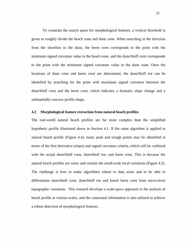
4.2 Morphological feature extraction from natural beach profiles
The real-world natural beach profiles are far more complex than the simplified
hypothetic profile illustrated above in Section 4.1. If the same algorithm is applied to
natural beach profile (Figure 4.4), many peak and trough points may be identified in
terms of the first derivative (slope) and signed curvature criteria, which will be confused
with the actual dune/bluff crest, dune/bluff toe, and berm crest. This is because the
natural beach profiles are noisy and contain the small-scale local variations (Figure 4.5).
The challenge is how to make algorithms robust to data noise and to be able to
differentiate dune/bluff crest, dune/bluff toe and beach berm crest from micro-level
topographic variations. This research develops a scale-space approach to the analysis of
beach profile at various scales, and the contextual information is also utilized to achieve
a robust detection of morphological features.

38
Figure 4.4 A natural beach profile
Figure 4.5 Slope and curvature derived for a natural beach profile

39
4.2.1 Scale-space approach to feature extraction from beach profiles
A successful extraction of the important morphological features from the natural beach
profiles depends upon the selection of appropriate scale of analysis. The need for a
multi-scale signal analysis method arises when we need to automatically derive
information from real world measurement (Lindeberg, 1994). The scale-space approach
(Witkin, 1983) is one of the most well-developed and commonly used methods of multi-
scale analysis, which can be used to represent a curve as a family of curves smoothed at
various detail levels. The essential requirement for multi-scale analysis is that new
structures, which do not correspond to the simplifications of corresponding structures at
finer scale, should not be created at a coarser scale. A set of standard scale-space axioms
has been used to derive the appropriate low-pass kernel type. The uniqueness of
Gaussian kernel result in its suitability for the scale-space approach, which includes
linearity, shift invariance, the semi-group structure, scale invariance, rotational
invariance, non-creation of local extrema, and non-enhancement of local extrema.
A Gaussian kernel follows the Gaussian distribution. For continuous variable x,
the standard Gaussian distribution )(xG with mean µ = 0 and standard deviation σ is
given by:
)2
exp(2
1),(
2
2
σσπσ x
xG −= (4.6)
Gaussian distributions centered at mean of zero with different standard deviations are
graphed in Figure 4.6. As shown, the larger the standard deviation valueσ , the more
spread out the kernel distribution is.

40
Figure 4.6 Gaussian distributions with different standard deviations
For a given curve u(x), its Gaussian scale-space representation is a family of
curves defined by its convolution with the Gaussian kernel with varying standard
deviation values:
),()(),( σσ xGxuxU ∗= (4.7)
The standard deviation σ controls the smoothing degree of the filter. The larger the
standard deviation, the larger the scale of analysis and the less details (local variations)
will remain in the curve.
The critical features of the elevation curve correspond to the points of dramatic
slope changes, which are associated with the extreme points on the curvature curve. By
selecting different standard deviation values for Gaussian filter, the elevation curve can
be smoothed at different scales, so that the critical features can be extracted at different
scale from the resulting curvature curve.
41
When dealing with elevation curve based on discrete distance measurements, the
Gaussian distribution ),( σnG needs to be discretized:
)2
)(exp(
2
1),(
2
2
σσπσ xn
nG∆−= n = KK ,2,1,0,1,2, −− (4.8)
where σ is standard deviation and x∆ is the cell size. Since the Gaussian function decays
rapidly, 95.45% of the area in the Gaussian function is contained in the window
[ 02σ− , 02σ ], given an analysis scale0σ . Therefore, to construct a discrete Gaussian
filter, the filter window could be truncated and be implemented as [ b− ,b ], where b is
the minimum integer that satisfies 02σ≥∆xb . For each pixel ∈n [ b− ,b ] in the filter
window, its value for the Gaussian filter could be calculated as:
)2
)(exp(
2
1),( 2
0
2
0
0 σσπσ xn
nG∆−= n = bbbb ,1,,1,0,1,,1, −−+−− KK (4.9)
Given the elevation curve )(nfz = , the smoothed curve of )(nf at specific
scale 0σ is defined by its convolution with the Gaussian kernel:
),()(),( 00 σσ nGnfnF ∗= = ),()( 0σmnGmfb
bm
−∗∑−=
(4.10)
n = bbbb ,1,,1,0,1,,1, −−+−− KK
After smoothing elevation curve )(nfz = at scale 0σ , the first derivative, second
derivative, and curvature could be calculated for the smoothed elevation curve ),( 0σnF .
The critical features of the elevation curve could be identified as extreme points on
curvature curve at various analysis scales.

42
For example, when a Gaussian filter with standard deviation σ =1 is applied to
smooth the elevation curve shown in Figure 4.4, the resulting slope and curvature curves
(Figure 4.7) are much smoother than the results from the original elevation dataset
(Figure 4.5). On the curvature curve, the points corresponding to the critical features
could be recognized as the extreme points, although there are some local extreme points
in the neighborhood with very high curvature value, which may still cause confusion in
the feature extraction process.
Figure 4.7 Feature extraction of beach profile at smooth scale σ =1
When a Gaussian filter with standard deviation σ =2 is applied to smooth the
elevation curve shown in Figure 4.4, the resulting slope and curvature curve are even
more smooth (Figure 4.8). On the curvature curve, the points corresponding to the

43
important features could be easily distinguished as the extreme points, and there is
almost no local extreme point in the neighborhood that could cause confusion when
identifying the important features.
Figure 4.8 Feature extraction of beach profile at smooth scale σ =2
When a Gaussian filter with standard deviation σ =4 is applied to smooth the
elevation curve shown in Figure 4.4, the slope and curvature curve are further smoothed
(Figure 4.9). On the curvature curve, the points corresponding to the important features
still can be recognized as the extreme points, but are not as distinctive as they were when
σ =2. Besides, the extreme points shift from the locations that exactly correspond to the
original slope change point of the elevation curve, which is caused by the larger analysis
window.

44
Figure 4.9 Feature extraction of beach profile at smoothing scale σ =4
Overall, analyzing the original beach profile at different detail levels will create
different results for feature extraction. At a small scale of analysis, the local variations of
elevation curve will result in the unwanted fluctuations in the slope and curvature curve,
which may cause difficulty in distinguishing the critical feature points from many other
local extreme points in the neighborhood. By increasing the scale of analysis, the
curvature curve will become smoother, which will make the points that correspond to
critical features more prominent. However, when the scale of analysis is further
increased and becomes too large, the original elevation curve will be over smoothed,
which may result in serious shift of the detected location of the critical features or even
the failure in detecting certain features. The determination of appropriate scale of
analysis is critical to achieve a desired result of beach profile feature extraction.
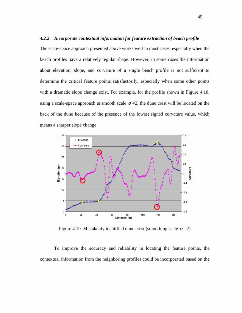
45
4.2.2 Incorporate contextual information for feature extraction of beach profile
The scale-space approach presented above works well in most cases, especially when the
beach profiles have a relatively regular shape. However, in some cases the information
about elevation, slope, and curvature of a single beach profile is not sufficient to
determine the critical feature points satisfactorily, especially when some other points
with a dramatic slope change exist. For example, for the profile shown in Figure 4.10,
using a scale-space approach at smooth scale σ =2, the dune crest will be located on the
back of the dune because of the presence of the lowest signed curvature value, which
means a sharper slope change.
Figure 4.10 Mistakenly identified dune crest (smoothing scale σ =2)
To improve the accuracy and reliability in locating the feature points, the
contextual information from the neighboring profiles could be incorporated based on the

46
assumption that the horizontal distance from origin point and the elevation of feature
points are continuous or change gradually along a small segment of shoreline.
For the dune crest point identified based on curvature property for the profile
shown in Figure 4.10. Its elevation and the horizontal distance from the shoreline are not
consistent and compatible with its neighbors (Figure 4.11).
Figure 4.11 Example of dune crest identification based on information from individual beach profile. (a) Mistakenly identified dune crest (Profile ID = 170); (b) Inconsistency in horizontal distance from shoreline; (c) Inconsistency in elevation values
To incorporate the contextual information from the neighboring profiles, the
compatibility and consistency analysis is performed for morphological points extracted
for each beach profile in comparison with its neighboring profiles. If a dramatic
difference exists between the location (horizontal and/or vertical) of its dune crest and
the neighboring dune crests, the current location of the dune crest on profile is identified

47
as a potential error. Then several other locations which meet the elevation and curvature
criteria are selected as candidate dune crest points on the beach profile. The
compatibility of each candidate dune crest point with the dune crests on neighboring
profiles is calculated based on both the horizontal distance to the origin point and the
elevation. The dune crest point will be adjusted to the candidate location with most
compatible horizontal distance and elevation value. Gaussian distribution is assumed for
both the horizontal distances and elevation values of the dune crests of beach profiles
within a given neighborhood of the shore segment. For each individual beach profile, the
algorithms are as follows:
Step 1: Calculate the means and standard deviations of elevation and horizontal distance
of the neighboring dune crest points in the given neighborhood:
∑=
=N
i
iDCDC z
Nz
1
1 (4.11)
∑=
=N
i
iDCDC x
Nx
1
1 (4.12)
where N is the total number of neighboring profiles in the given window size. DCz is the
average elevation of all the neighboring dune crests in this given window; iDCz is the
elevation of the dune crest on profile i. Similarly, DCx is the average horizontal distance
from each neighboring dune crests to its corresponding origin point; iDCx is the
horizontal distance from the dune crest on profile i to its origin point.
∑=
−−
=N
iDC
iDCDC zz
Nz
1
2)(1
1)(σ ∑
=
−−
=N
iDC
iDC zNz
N 1
22 ])()([1
1 (4.13)

48
∑=
−−
=N
iDC
iDCDC xx
Nx
1
2)(1
1)(σ ∑
=
−−
=N
iDC
iDC xNx
N 1
22 ])()([1
1 (4.14)
where N is the total number of neighboring profiles in the given window size; )( DCzσ is
the standard deviation of elevation of all the neighboring dune crests in the given
neighborhood; )( DCxσ is the standard deviation of horizontal distance from all the
neighboring dune crests to the corresponding origin point.
Step 2: Determine if the elevation and/or horizontal distance of the dune crest is
compatible with its neighborhood. UseDCz to denote the elevation of the dune crest on
current profile, and DCx to denote the horizontal distance from the dune crest to its
origin point. The location of the dune crest will be identified as incompatible if the
difference between the current location and the mean value of the neighborhood exceeds
a certain threshold, i.e.:
)(|| DCDCDC zkzz σ≥− or
)(|| DCDCDC xkxx σ≥− (4.15)
where k is the multiplicative factor (usually ranging from 1.0 to 3.0). Once a dune crest
location is identified as incompatible and thus may need to be adjusted, the following
steps need to be executed.
Step 3: Determine the candidate locations for dune crest. The candidate location for
dune crest could be selected based on combination of several criteria: (1) having an
elevation above the minimum threshold; (2) having a signed curvature value lower than
the maximum threshold; and (3) being the local minimum curvature point.

49
Step 4: Calculate the compatibility of each candidate dune crest with other dune crests
on the neighboring profiles based on Gaussian distribution.
The probability density function of the standard Gaussian distribution with mean
µ = 0 and standard deviation σ =1 is given by:
)2
exp(2
1)(
2
1,0
xx −=
πϕ (4.16)
The cumulative distribution function of a probability distribution is the probability of the
event that a random variable X with that distribution is less than or equal to x. The
cumulative distribution function of standard Gaussian distribution is given by:
duu
xxXPx
∫ ∞−−=Φ=≤ )
2exp(
2
1)()(
2
1,01,0 π (4.17)
Thus the probability of the event that a random variable X with standard Gaussian
distribution has an absolute value larger than x is:
)(2)(1)( 1,01,01,0 xxXxPxXP −Φ=<<−−=> (4.18)
For a random variable X that follows Gaussian distribution with mean µ and standard
deviationσ , the probability of the event that X has an absolute value larger than x is:
)(2)()( 1,01,0 σµ
σµ
σµ −−Φ=−>−=> xxX
PxXP (4.19)
When x equals toµ , the probability equals to 1. The larger the distance of x from mean
value µ , the lower the probability of the event that X has an absolute value large than x ,
and the probability is approaching to 0 when x is moving further away from the mean
value µ .

50
Assuming the elevation and horizontal distance measurements of dune crest
follows Gaussian distribution, the normalized measurements follows a standard
Gaussian distribution, which means:
))(
(2)( 1,0DC
DCDCDC z
zzzZP
σ−−Φ=> (4.20)
))(
(2)( 1,0DC
DCDCDC x
xxxXP
σ−−Φ=> (4.21)
The compatibility of the dune crest on current beach profile with the dune crests in the
neighborhood could be derived based on both the elevation and horizontal distance
measurements:
))(
(4)()( 1,0DC
DCDCDCDCDC z
zzxXPzZPQ
σ−−Φ=>>= )
)((1,0
DC
DCDC
x
xx
σ−−Φ (4.22)
The commonly used algorithm to approximate the cumulative distribution function of
standard Gaussian distribution is from Abramowitz and Stegun (1964). Given:
)2
exp(2
1)(
2
1,0
xx −=
πϕ (4.23)
The cumulative normal distribution is given by:
εϕ +++++−=Φ ))((1)( 55
44
33
2211,01,0 tbtbtbtbtbxx (4.24)
where )2316419.01/(1 xt += , 1b =0.319381530, 2b =-0.356563782, 3b = 1.781477937,
4b = -1.821255978, 5b = 1.330274429. This approximation has a maximum absolute
error of 85.7 −e .
Step 5: Adjust the dune crest point to the location that has the highest compatibility.

51
As shown in Figure 4.10, the compatibility function is calculated for the local
minimum points which satisfy the requirement of elevation and curvature (in this case
elevation > 10m and curvature < -0.1). The local minimum point with the highest
compatibility value is identified as dune crest (Figure 4.12 and Table 4.1). The relocated
dune crest is more consistent with its neighbors in terms of elevation and distance from
origin point on the shoreline (Figure 4.13).
Figure 4.12 Adjustment of dune crest location using compatibility values
Table 4.1 Compatibility values calculated based on contextual information
Local minimum point
Curvature Distance (meter)
Elevation (meter)
Compatibility
1 -0.3505 119 31.79 0.00064 2 -0.2569 54 12.45 0.00021 3 -0.2336 82 30.12 0.25300 4 -0.1101 136 23.97 1.91E-05

52
Figure 4.13 Example of dune crests identification. (a) Comparison between dune crests identified before and after incorporating contextual information; (b) Improved consistency in horizontal distance from origin point; (c) Improved consistency in elevation values
Using the similar algorithm, the location of the beach berm crest of each profile
can be adjusted by incorporating the contextual information. Then the dune toe can be
relocated based on the updated location of berm crest and dune crest.

53
4.2.3 Procedures for deriving morphologic attributes for beach profiles along the
shoreline
The traditional ground survey transects are approximately perpendicular to the shoreline.
Similarly, to automatically generate beach profiles from LiDAR DEM, the first step is to
extract the shoreline as the reference to orientate transects. Shoreline is the spatially
continuous line of contact between the land and the sea. More accurately, shoreline is
defined as the intersection line between the land and the mean high water level (MHWL).
This definition is adopted by many US agencies such as the United States Army Corps
of Engineers, Federal Emergency Management Agency, and U.S. Census Bureau
(Graham et al., 2003). Based on LiDAR elevation data, shoreline can be extracted using
object-based or contour-based approach. In most cases, the shoreline extracted from high
resolution LiDAR data contains too much spatial detail for generating perpendicular
transects. The shoreline needs to be smoothed to eliminate the unnecessary details to
ensure the orientation of transects vary smoothly and gradually.
After the shoreline is extracted and smoothed, the location of the starting point of
each transect can be determined along the shoreline at a regular interval. The length of
the transects can be specified according to the practical needs at particular study area.
The orientation of each transect is calculated based on the local segments of the
shoreline. A moving window with a selected size is centered at the starting point of each
profile. A linear regression line is fit for the shoreline within the window. The
orientation of the profile is then set to be perpendicular to this local regression line.

54
After the transects are located, the corresponding elevation values can be
extracted from the LiDAR DEM along each transect line. The Gaussian filter at
optimum scale is applied to smooth the elevation curve. The first derivative, second
derivative, and curvature are then derived for the smoothed elevation curve to extract the
critical beach features from each individual beach profile. Then the contextual
information from the neighborhood of each beach profile can be incorporated to identify
the feature points that are not consistent with its neighbors in terms of elevation and/or
horizontal distance. The locations of those incompatible feature points can be adjusted
based on the compatibility analysis of candidate locations.
After the feature points for each beach profile are derived, the feature points on
beach profile and the segments between feature points can be converted from raster-
based grid format to vector-based point and polyline format. Both the raster and vector
representations of the points and segments of the profile are maintained in the database.
For raster representation, each profile is stored as a series of grid cells with the ID
number of feature points. For vector representation, the feature points and segments are
located on the profile using linear referencing and dynamic segmentation techniques. By
definition, linear referencing is the method of storing geographic location by using
relative positions along a measured linear feature, while the dynamic segmentation refers
to the process of calculating the absolute locations of events using linear referencing
system and locating them on the map (Brennan and Harlow, 2002). First, a route can be
created from each profile line by using profile length to accumulate the route measures.
Then a point event table can be created for all the feature points, which records the ID of

55
the profile that each point belongs to, as well as the distance of the feature point to the
origin point of the profile. At last, a route event layer can be generated based on profile
routes and point event table by linking the points to the corresponding profile using route
ID, and locating the points on the profile using its distance from the origin point as
measure values. Similarly, a line event table can be created for all the segments between
feature points. A route event layer can be generated using profile routes and line event
table by linking each segment to its corresponding profiles using route ID, and locating
the segments on the profile using the distance measurement of its from-point and to-
point. Compared to raster representation, the vector format of feature points and
segments of profile is much easier to be displayed, edited, and analyzed in a GIS
environment in association with other data layers.
4.2.4 Derivation of attributes for characterizing beach profiles and profile changes
Based on the object representation of feature points and segments of each profile, a set
of attributes can be extracted to support a detailed quantitative analysis of coastal
morphology in the cross-shore direction. For beach feature points such as berm crest,
dune crest, and dune toe, the elevation of the points and their horizontal distance from
the origin point of corresponding profile can be calculated. For segments between the
point features, such as dune face and beach berm, the corresponding height, width, and
slope of each segment can be derived.
If time series of profiles from repeat LiDAR surveys are available, the magnitude
of changes can be calculated for each attributes, such as the horizontal and vertical
displacement of each feature point, as well as the change in height, width, and slope of

56
each segment along the profile. The dune volumetric change is calculated based on the
horizontal position of pre-surface dune toe and the dune crest location that is furthest
from shoreline among different time periods. Limited by the water penetration ability of
topographic LiDAR system, the beach volumetric change can only be calculated from
the position of shoreline to the horizontal position of pre-surface dune toe.
4.3 ArcGIS extension module for beach profile analysis
To support the beach profile feature extraction and attribute derivation, an ArcGIS
extension module – Profile Analyst, is developed in the environment of Microsoft Visual
Studio .NET 2003. The core algorithms are programmed as a series of DLLs using the
C++ language, and the graphical interface is developed by VB .NET and the relevant
ArcObjects. This extension module can be used seamlessly with ArcGIS package. The
graphical interface for Profile Analyst is shown in Figure 4.14. The capabilities of this
module include:
(1) Generate cross sections: This software routine has a customized dialogue menu
which guides the user to load the input data and to set the relevant parameter values to
delineate cross sections (Figure 4.14b). The required input data are LiDAR DEM and
shoreline, which may be extracted or digitized based on LiDAR data and /or high-
resolution remote sensing imagery. The parameters to be specified include the beach
profile length and profile interval. Transects perpendicular to the shoreline can be
automatically generated at the specified interval. The elevation values for all the grids on
each transect can be sampled from the LiDAR DEM and be stored as a list in memory.

57
Figure 4.14 ArcGIS extension module – Profile Analyst. (a) Pull-down menu for the extension module; (b) Dialogue form for generating cross sections; (c) Dialogue form for extracting feature points from single profile; (d) Dialogue form for extracting feature points for all profiles; (e) Dialogue form for editing feature points; (f) Dialogue form for calculating morphologic attributes; (g) Dialogue form for generating cross sections for change analysis; (h) Dialogue form for comparing profiles; (i) Dialogue form for calculating change attributes;(j) Dialogue form for calculating volumetric attributes; (k) Dialogue form for visualizing morphological changes along shoreline

58
Figure 4.14 (Continued)

59
Figure 4.14 (Continued)

60
(2) Interactively extract feature points from single profile: This routine allows the
user to preview selected profile curve and to determine appropriate parameters for
feature extraction (Figure 4.14c). First, the selected profile curve can be displayed. The
standard deviation value can be set for the Gaussian filter to smooth the original
elevation curve at different scales, and the resulting signed curvature curve can be
displayed in a separate window. By setting a vertical threshold to roughly divide the
profile into beach zone and dune zone, the resulting feature points could be derived and
displayed on the beach profile. After several experiments on various profiles, the
optimum scale of analysis and the elevation threshold can be determined. The elevation
values along the profile and the coordinates for identified feature points can be exported
to Excel for a detailed analysis.
(3) Extract feature points for all profiles: After the optimal parameters are determined
based on experiments on representative profiles, this software routine allows users to
apply these parameters for the case study area to extract critical features (Figure 4.14d).
Feature points can be extracted based on geometric information of each individual beach
profile, and can also be adjusted by incorporating the contextual information from the
neighboring profiles. To incorporate the contextual information, the user needs to set the
number of profiles in the neighborhood to calculate the compatibility value.
The resulting feature points such as beach berm crest, dune/bluff crest and
dune/bluff toe are initially stored in memory as distance-elevation pair for each profile.
By using a set of ArcObjects related to linear referencing and dynamic segmentation in

61
ArcGIS, the feature points and segments can be saved in event tables and be displayed in
vector format.
(4) Edit feature points: After the automatic profile feature extraction, the manual
editing can fix feature points that are not correctly located by the automatic algorithms
(Figure 4.14e). For a selected profile, the distance-elevation pair of feature points can be
read from the feature point layer created by previous steps and be displayed on the
corresponding elevation curve. With this software routine, the location of the feature
points can be interactively edited, added, or deleted. The feature point layer can be
updated after the new location of feature point is determined.
(5) Calculate morphologic attributes: After the automatic feature extraction and
manual editing, a set of morphological attributes can be derived for each beach profile
(Figure 4.14f). The attributes for feature point include the elevation and the horizontal
distance to the shoreline. The attributes for dune/bluff face and beach berm include the
height, width, and slope. The feature points of the same type can be connected to form
the feature line, such as dune crest line, dune toe line, and berm crest line.
(6) Generate cross sections for change analysis: This routine allows user to perform
change analysis between two successive LiDAR surveys (Figure 4.14g). The user can
specify the two LiDAR DEMs to be compared and the reference shoreline. Similar to the
single DEM analysis, the user is allowed to set the beach profile length and profile
interval. After transects are generated, the elevation values can be extracted for two
DEMs along each transect.

62
(7) Compare profiles: This routine allows user to compare the elevation profiles
measured at two different time periods (Figure 4.14h). The identified feature points can
be displayed on the profiles to reveal their displacements. The cut and fill areas can be
displayed on the cross-shore view and the total volumetric change for each profile can be
calculated.
(8) Calculate change attributes: This routine allows user to calculate the attribute
changes during the temporal span between two LiDAR surveys (Figure 4.14i). The
change attributes include the horizontal distance and elevation changes for feature points,
as well as the height, width, and slope change for dune/bluff face and beach berm. The
volumetric change attributes are also derived for beach and dune sections (Figure 4.14j).
(9) Spatial pattern of profile feature attributes and change attributes: This routine
facilitates the visualization of the spatial variations of morphologic attributes for each
survey and the analysis of change attributes between two surveys (Figure 4.14k).
Several attributes can be selected and displayed at the same time, which is helpful in
interpreting and analyzing coastal morphological change patterns.

63
5 OBJECT-BASED METHOD FOR MORPHOLOGICAL AND
VOLUMETRIC CHANGE ANALYSIS
This section presents the object-based method for morphological and volumetric change
analysis. The object-oriented method represents a two-dimensional approach to the
analysis of coastal morphology and its changes. The basic spatial units for object-
oriented analysis method are the erosion and deposition patches and zones, in contrast to
the profiles in the one-dimensional profile analysis approach. This section starts with the
presentation of algorithms for identifying and delineating the positive change and
negative change objects. Then, algorithms and software tools are presented for deriving
attributes for characterizing these morphological change objects.
5.1 Identification and delineation of elevation change objects
The main procedures of change object identification and delineation include three steps:
pixel-based elevation differencing, morphological change classification, and object
identification.
For change analysis, LiDAR surveys at two different times for the same region
needs to be preprocessed, including geo-referencing, horizontal co-registration, vertical
adjustment, and low-pass filtering. Then, the two LiDAR DEMs can be differenced for
change analysis as in Equation (5.1):
12 tij
tijij zzz −=∆ (5.1)
where 1tijz and 2t
ijz are the elevation measurements for the cell (i, j) respectively at the
early time t1 and the late time t2, and ∆zij is the elevation difference for the cell (i, j). A

64
positive elevation difference value indicates that the surface materials have been added
at this location, while a negative elevation difference value indicates that the surface
materials have been removed (Figure 5.1c).
Figure 5.1 Identification of elevation change objects. (a) DEM at the time t2; (b) DEM at the time t1; (c) Elevation difference values; (d) Morphological change classification values; (e) Resulting objects with ID numbers
In the resulting pixel-based elevation difference imagery, the cells with elevation
change value can be further classified into three morphological change categories:
positive change cells, negative change cells, and unchanged cells (Figure 5.1d). As
discussed in Section 3, “Unchanged” can be defined as the case when elevation change
value is within a range of the measurement error. Given dσ as the random error for
elevation difference measurements and k as the multiplicative factor (usually ranging
from 1.0 to 3.0), the elevation differencing image could be reclassified into three
categories: positive change (1), negative change (-1), and unchanged (0) according to
Equation (5.2):

65
dijd
dij
dij
ij
kzkif
kzif
kzif
c
σσσ
σ
<∆<−−<∆
>∆
−=,0
,1
,1
(5.2)
where ijc is the morphological change code for the grid cell (i, j).
In this object-based volumetric change analysis method, the unchanged cells are
considered as background and the individual positive change and negative change
patches are considered as objects (Figure 5.1e). For example, a positive change object is
defined as a continuous spatial aggregation of cells with a positive elevation change
value, in which any two cells are spatially connected. Two cells are considered to be
spatially connected if there exits a path between two cells that consists of a series of
adjacent cells. In this case, two cells are defined as adjacent to each other when one cell
is the four immediate neighbor of the other. A recursive connected-component
expansion algorithm (Sonka et al., 1999; Liu and Jezek, 2004) is used to identify and
index positive change objects based on the spatial connectivity of cells. First, the
elevation difference grid is scanned in a row-wise manner, and a seed is set at the first
cell with a positive elevation change value. Second, this seed is expanded to include all
the positive change cells located in the four immediate neighborhood of the current cell.
The expansion is continued recursively until all the spatially connected positive change
cells are included in the current patch. In this way, the first positive change object is
delineated and indexed. As repeating this recursive expansion process to identify
positive change objects one-by-one, the objects are indexed incrementally with a unique
identification number. Following the same procedure, the negative change objects could

66
be delineated and indexed. Positive (negative) change objects with different
identification numbers are spatially detached to each other, which is guaranteed by the
algorithm. However, a positive change object and a negative change object might be
adjacent to each other. As a final result, the recursive connected-component expansion
algorithm creates a series of discrete elevation change objects which are embedded in the
background of unchanged cells.
When applying the algorithm to real LiDAR data, the identification of objects
may be subject to errors for various reasons such as data noise, residual horizontal
alignment error, and resolution limitation during image acquisition. The delineated
objects may have small holes and breaks, and their boundaries may have a rough and
jagged shape. To generalize the shape of the objects, three steps of morphology
operations are applied. First, a closing operation (Sonka et al., 1999) is applied to
smooth the object boundaries and close the small gaps in objects. The closing operation
consists of a dilation operation followed by an erosion operation. The dilation operation
adds cells to the perimeter of each object, and thus potentially closes broken areas.
Erosion operation etches cells away from the perimeter of each object and therefore
shrinks the object. Second, a fill operation is applied to close small interior holes and
cavities whose size is smaller than a specified threshold. Third, a trim operation is
applied to eliminate those isolated objects whose size is smaller than the specified
threshold.
After the discrete objects are generalized by the morphologic operations, they are
converted from raster-based grid format to vector-based polygon format. Both the raster

67
and vector representations of the objects are maintained in the database. For raster
representation, each object is stored as a list of spatially-connected grid cells with a same
identification number, and the object attributes are stored in an associated attribute table
with the same identification number. For vector representation, each object is stored as a
polygon, and a feature attribute table is associated with the polygon layer. The feature
attribute table contains object identification numbers and various spatial and volumetric
properties of corresponding objects as described in the next section. The vector format of
elevation change objects can be directly displayed, edited and analyzed in a GIS
environment in association with other data layers.
5.2 Attribute derivation for characterizing erosion and deposition objects
Based on the object representation of elevation change patches, a set of spatial and
volumetric attributes can be derived to support a detailed quantitative analysis of coastal
morphology change. Individual elevation change patch is treated as the basic spatial
units for morphological and volumetric change analysis. First, the internal composition
and heterogeneity for each object can be characterized by a set of variables. For example,
the range and standard deviation of vertical elevation changes could describe the internal
heterogeneity of elevation changes within an object. Second, each object could be
treated as homogenous entities and be characterized by a set of spatial and volumetric
properties. Third, the spatial pattern of erosion and deposition objects could be measured
by aggregation and distribution properties, over specified sub-regions or across the entire
landscape.

68
From successive LiDAR datasets, five categories of attributes are calculated for
each elevation change object, which include planimetric attributes, shape attributes,
surface attributes, volumetric attributes, and summary statistical attributes. The
combination of these attributes could provide comprehensive quantitative information
for investigating morphological and volumetric characteristics of elevation change
patches. Thematic attributes could also be calculated for each object if other ancillary
data sources such as multi-spectral remote sensing imagery are incorporated. A
combination of various attributes could facilitate the classification of elevation changes
caused by different mechanisms.
This research aims at providing an analytical framework and software tool for
object-based morphological and volumetric change analysis, so that a large list of
attributes are deduced and calculated. For specific research purpose or specific study
area, the users may select the attributes that are most useful for characterizing particular
aspects of coastal morphology.
5.2.1 Planimetric attributes
The planimetric attributes describe the geographical position, horizontal dimensions and
size of the elevation change objects. Those include the coordinates ( yx, ) of centroid
point, perimeter (p), area (A), thickness (THK), as well as the length (l) and width (w) of
the minimum bounding rectangle. The numerical definitions of these attributes are listed
in Table 5.1. The centroid point is the gravity center of the object and indicates the
geographical location of the object. The perimeter measures the length of the object
boundary. The thickness of an object is defined as the maximum distance of interior cells

69
of the object to its nearest boundary, namely the distance of the deepest cell inside the
object to its boundary. The length and width of the minimum bounding rectangle gives
the measurements on the horizontal dimensions of the object.
Table 5.1 Definitions of planimetric attributes Attributes Definition
Centroid point ( yx, ) ∑
=
=n
i
ixn
x1
)(1
; ∑=
=n
i
iyn
y1
)(1
n is the number of cells consisting of an object, (xi, yi) are the horizontal and vertical coordinates of the ith cell of the object
Perimeter (P)
rmrmp 21 2+=
m2 is the number of boundary cell in diagonal step, m1 is the number of boundary cell in horizontal or vertical orientation, and r is the grid cell size
Area (A)
2nrA =
n is the number of cells consisting of an object, and r is the grid cell size.
Thickness (THK) }max{ idTHK =
di is the distance of the cell i to the nearest boundary.
Length (l) length of the minimum bounding rectangle enclosing the object
Width (w)
width of the minimum bounding rectangle enclosing the object
5.2.2 Shape attributes
Shape attributes describe the planar geometric shape of the objects. Due to the
differences in the nature of changes and diverse coastal processes, the elevation change
objects may have different shape characteristics and complexity. Some have compact
forms, while others have narrow and elongated shapes. Some have simple, regular, and

70
smooth boundaries, while others have convoluted, rugged and complex boundaries. The
different shape characteristics of elevation change objects could be used to facilitate the
inference of the underlying coastal processes. A set of attributes are calculated for
characterizing different aspects of the shape property, including compactness index (CI),
elongatedness (ELG), asymmetry (ASM), orientation (φ ), fractal dimension (D),
rectangularity (REC), ellipticity (ELP), and triangularity (TRI) (Table 5.2).
Compactness index (CI) is a widely used shape indicator (Davis, 2002), which is
defined based on the perimeter and area measure of the object. The most compact object
in a Euclidean space is a circle. A circle-shaped object has a compactness index of one,
and so that the compactness index is also known as the circularity measure (Pratt, 1991).
Elongatedness is defined as a ratio between the length and width of the fitted minimum
bounding rectangle. The circle and square have the smallest value for the elongatedness,
which equals to one. The asymmetry is defined based on the best-fit ellipse of the object,
which is the ratio of the major and minor axes of the ellipse. The circle and square have
an asymmetry value of zero. The orientation is defined as an angle in degree between the
horizontal axis and the major axis of the best-fit ellipse measured counterclockwise from
0 to 180.
Rectangularity, ellipticity and triangularity respectively measure the similarity of
the shape of an object to typical rectangle, ellipse and triangle shapes. The rectangularity
is defined by the ratio between the area of the object to the area of the minimum
bounding rectangle. The ellipticity and triangularity are defined based on the affine
moment invariant (Flusser and Suk, 1993; Rosin, 1993). All the rectangularity, ellipticity,

71
and triangularity values range from 0 to 1. The larger the value, the more similar an
object is to the corresponding typical shape.
Table 5.2 Definitions of shape attributes Attributes Definition
Compactness index (CI) 2
4
p
ACI
π=
Elongatedness (ELG) w
lELG =
Asymmetry (ASM)
a
bASM −= 1 ∑
−−−=
n
i
qi
pipq yyxx
n 1
)()(1µ
00
211
202200220 )4)((2
µµµµµµ +−++
=a
100
211
202200220 )4)((2
µµµµµµ +−−+
=b
a and b are the semi-major and semi-minor of the best-fit ellipse, µpq are the central moments.
Orientation (φ)
−= −
0220
111 2tan
2
1
µµµφ
µpq are the central moments.
Fractal dimension (D)
DcrrN −= 1)(
r is the width of box, N(r) is the counts of the boxes contain the object.
Rectangularity (REC) lw
AREC=
Ellipticity (ELP)
≤=
otherwise 16
1 if 16
12
161
112
2
I
IIELP
π
π π
400
2110220
1 µµµµ −=I
µpq are the central moments and I1 is the affine moment invariant.
Triangularity (TRI)
≤= otherwise
108
1 if 108
1
1081
11
I
IITRI
I1 is the affine moment invariant.

72
The shape complexity of object boundary can be measured in terms of a
perimeter-to-area ratio or fractal dimension (Mandelbrot 1983, Burrough 1981). Both the
perimeter-to-area ratio and the fractal dimension increase with the increasing complexity
of the object boundary. The problem with the perimeter-area ratio method is that it is
size dependent. For two objects of the same shape, the larger object has a lower
perimeter-area ratio than that of the smaller object. To avoid the size dependency
problem of perimeter-area ratio, the fractal dimension is selected as the indicator to
measure the complexity of object boundary. The fractal dimension is calculated for each
object using the box-counting method, which includes the following steps (Foroutan-
pour, 1999):
Step 1: Use a grid with a cell size ir to cover the object, and then count the number of
cells iN that contain part of the boundary of object.
Step 2: Vary the cell size and record a series of counts { 1r , 1N }, { 2r , 2N }, …, { mr , mN }.
Step 3: Fit a linear regression line of points { )log( 1r , )log( 1N }, { )log( 2r , )log( 2N }, …,
{ )log( mr , )log( mN }.
Step 4: Determine the fractal dimension D using the linear regression equation:
)log()log())(log( rDKrN += (K is a constant) (5.3)
To generalize the shape and orientation of each object, a minimum bounding
rectangle could be fitted to enclose the object, which is the smallest rectangle that
contains all cells of the object and aligned with the major and minor principal axes of the

73
object (Figure 5.2). The algorithms of determining minimum bounding rectangle include
the following steps (Chaudhuri and Samal 2007; Suesse and Voss, 2001):
Step 1: Compute the centroid point (yx, ) of object and the angle of the major axis with
the horizontal axis θ (Figure 5.3a).
Step 2: Compute the upper and lower furthest boundary points with respect to both
major and minor axes (Figure 5.3b). Each boundary point ( ii yx , ) can be
classified to be upper, lower, and on with respect to the major axis using:
)(tan)( xxyyV ii −−−= θ (5.4)
Boundary point ( ii yx , ) is an upper boundary point with respect to major axis
when V > 0, a lower boundary point when V < 0, and on the major axis if V = 0.
Then the upper and lower furthest boundary points with respect to major axis
could be determined within each groups. Similarly, by using
)(cot)( xxyyU ii −+−= θ , the upper and lower furthest boundary points with
respect to minor axis could be determined.
Step 3: Compute the vertices of the four corners of the minimum bounding rectangle
(Figure 5.3c). Let ( 11, yx ) and ( 22, yx ) be the upper and lower furthest boundary
points with respect to major axis, and let ( 33, yx ) and ( 44, yx ) be the upper and
lower furthest boundary points with respect to minor axis. The vertices are
determined by finding the intersections of four lines: two lines are parallel to
major axis and respectively pass through (11, yx ) and ( 22, yx ); another two lines

74
are parallel to minor axis and respectively pass through ( 33, yx ) and ( 44, yx ). The
resulting coordinates of the four corners are:
Top left corner A:
θθ
θθcottan
cottan 1331
+−++= yyxx
x (5.5)
θθ
θθcottan
tancot 1331
+−++= xxyy
y (5.6)
Top right corner B:
θθ
θθcottan
cottan 1441
+−++= yyxx
x (5.7)
θθ
θθcottan
tancot 1441
+−++= xxyy
y (5.8)
Bottom left corner C:
θθ
θθcottan
cottan 2332
+−++= yyxx
x (5.9)
θθ
θθcottan
tancot 2332
+−++= xxyy
y (5.10)
Bottom right corner D:
θθ
θθcottan
cottan 2442
+−++= yyxx
x (5.11)
θθ
θθcottan
tancot 2442
+−++= xxyy
y (5.12)
Step 4: Connect the corresponding vertices to get the minimum bounding rectangle of
the current object.

75
Figure 5.2 A minimum bounding rectangle and its parameters
(a) (b) (c)
Figure 5.3 Steps of fitting minimum bounding rectangle. (a) Centroid and axes; (b) Upper and lower furthest points; (c) Vertices of minimum bounding rectangle
The best-fit ellipse of an object can be determined using all the cells within the
object (Figure 5.4). The center of the ellipse is located at the centroid point. The
principal axes of the ellipse are the eigenvector of the covariance matrix obtained by
treating the cells within the object as random variables. The major principal axis
corresponds to the eigenvector of the larger eigenvalue. Three parameters of the ellipse
including semi-major axis (a), semi-minor axis (b), and orientation (φ) can be calculated

76
using the lower-order central moments of the objects (Teague, 1980; Mulchrone and
Choudhury, 2004). The algorithms of determining best-fit ellipse include the following
steps:
Step 1: Compute the centroid point (yx, ) of the object.
Step 2: Compute the central moments of the object:
qi
n
i
pipq yyxx )()(
1
−−=∑=
µ (p = 0, 1; q = 0, 1) (5.13)
Step 3: Compute the semi-major axis, semi-minor axis, and orientation of the ellipse
11
211
202200220 )4)((2
µµµµµµ +−++
=a (5.14)
11
211
202200220 )4)((2
µµµµµµ +−−+
=b (5.15)
−= −
0220
111 2tan
21
µµµφ (5.16)
Step 4: Draw the best-fit ellipse.
Figure 5.4 Best-fit ellipse and its parameters

77
5.2.3 Surface attributes
Surface attributes describe the three-dimensional surface morphology and its changes in
terms of slope, aspect and curvature. To support the exploration of the interaction and
relationship between surface geomorphology and the coastal processes, a set of surface
attributes are calculated for each elevation change object, which includes: original-
surface average elevation (AV_EL1), subsequent-surface average elevation (AV_EL2),
average elevation difference (AV_EL_DIF), original-surface average slope (AV_SL1),
subsequent-surface average slope (AV_SL2), surface slope difference (AV_SL_DIF),
original-surface average aspect (AV_AS1), subsequent-surface average aspect (AV_AS2),
average surface aspect difference (AV_AS_DIF), original-surface curvature (AV_CV1),
subsequent- surface curvature (AVF_CV2), and average surface curvature difference
(AV_CV_DIF) (Table 5.3). The average value for surface elevation, slope (in percent
rise), or curvature for original and subsequent surfaces are simply calculated as the
arithmetic mean of all the cells within the object. The average value for surface aspect is
calculated through trigonometric operations as it is a circular direction measure in degree
(Davis, 2002). For aspect values1θ , 2θ , …, nθ , the average aspect is calculated as:
∑
∑
=
== n
ii
n
ii
R
1
1
cos
sinarctan
θ
θθ (5.17)

78
Table 5.3 Definitions of surface attributes Attributes Definition Original-surface average elevation (AV_EL1) Subsequent-surface average elevation (AV_EL2) Average elevation difference ( AV_EL_DIF)
∑=
=n
i
tizn
ELAV1
11
1_ ∑
=
=n
i
tiz
nELAV
1
22
1_
12 ____ ELAVELAVDIFELAV −=
1tiz and 2t
iz are the elevation of cell i of the object respectively at time t1 and t2
Original-surface average slope (AV_SL1) Subsequent-surface average slope (AV_SL2) Average slope difference ( AV_SL_DIF)
∑=
=n
i
tis
nSLAV
1
11
1_ ∑
=
=n
i
tis
nSLAV
1
22
1_
12 ____ SLAVSLAVDIFSLAV −=
1tis and 2t
is are the slope of cell i of the object respectively at time t1 and t2
Original-surface average aspect (AV_AP1) Subsequent-surface average aspect (AV_AP2) Average aspect difference ( AV_AP_DIF)
=∑
∑
=
=−n
i
ti
n
i
ti
APAV
1
1
1
1
11
cos
sintan_
θ
θ
=∑
∑
=
=−n
i
ti
n
i
ti
APAV
1
2
1
2
12
cos
sintan_
θ
θ
12 ____ APAVAPAVDIFAPAV −=
1tiθ and 2t
iθ are the aspect of cell i of the object respectively at time t1 and t2
Original-surface average curvature (AV_CV1) Subsequent-surface average curvature (AV_CV2) Average curvature difference ( AV_CV_DIF)
∑=
=n
i
tiv
nCVAV
1
11
1_ ∑
=
=n
i
tiv
nCVAV
1
22
1_
12 ____ CVAVCVAVDIFCVAV −=
1tiv and
2tiv are the curvature of cell i of the object respectively at time t1 and t2

79
5.2.4 Volumetric attributes
The volumetric attributes gives direct measurements on the magnitude and variation of
elevation change within an object, which include average vertical change (∆zav),
maximum vertical change (∆zmax), standard deviation of vertical change (∆zstd), vertical
change rate (ZR), volume change (VOL), and volume change rate (VR) (Table 5.4). The
average vertical change (∆zav) measures the central tendency of the elevation change for
each object. The maximum vertical change (∆zmax) and the standard deviation of vertical
change (∆zstd) measure the variation and the internal heterogeneity of the elevation
change within each object. The vertical change rate (ZR) quantifies the average elevation
change rate at a certain temporal scale. The volume change (VOL) and volume change
rate (VR) quantify the total change in the volume of surface material during the time
span between two surveys and the averaged change rate for each object.
5.2.5 Summary statistical attributes
After the erosion and deposition objects are identified based on a combination of
planimetrc, shape, surface, and volumetric attributes, summary statistics can be
calculated to quantify the extent, amount, spatial composition and configuration of
overall erosion, deposition, and net change for a certain region. Summary statistical
attributes include the number of erosion object (NUM_ER), average size of erosion
objects (AV_AREA_ER), total erosion area (AREA_ER), total erosion volume (VOL_ER),
the number of deposition object (NUM_DE), average size of deposition object
(AV_AREA_DE), total deposition area (AREA_DE), total deposition volume (VOL_DE),

80
net volume change (NET_VOL), and annual net volume change rate (NET_VOL_RT)
(Table 5.5).
Table 5.4 Definitions of volumetric attributes Attributes Definition
Average vertical change (∆zav)
∑=
∆=∆n
iiav z
nz
1
1
∆zi is the elevation change of cell i of the object
Maximum vertical change (∆zmax)
}max{max izz ∆=∆
Standard deviation of vertical changes (∆zstd)
2
1
)(1
1∑
=
∆−∆−
=∆n
iavistd zz
nz
Vertical change rate (ZR)
t
zZR av
∆∆=
∆t is the elapsed time between two successive topography surveys (t2-t1)
Volume change (VOL)
∑=
∆=n
iizrVOL
1
2
r is the grid cell size
Volume change rate (VR) t
VOLVR
∆=

81
Table 5.5 Definitions of summary statistical attributes Attributes Definition
Number of erosion objects (NUM_ER) Number of deposition objects (NUM_DE)
NUM_ER = Number of erosion objects
NUM_DE = Number of deposition objects
Total erosion area (AREA_ER)
Total deposition area
(AREA_DE)
∑=
=ERNUM
j
ejAERAREA
_
1
_
∑=
=DENUM
j
djADEAREA
_
1
_
Aej is the area of the jth erosion object
Adj is the area of the jth deposition object
Average size of erosion object (AV_AREA_ER) Average size of deposition object (AV_AREA_DE)
∑=
=ERNUM
j
ejA
ERNUMERAREAAV
_
1_
1__
∑=
=DENUM
j
ejA
DENUMDEAREAAV
_
1_1
__
Total erosion volume (VOL_ER)
Total deposition volume (VOL_DE)
∑=
=1
1
_n
j
ejVOLERVOL
∑=
=DENUM
j
djVOLDEVOL
_
1
_
VOL ej is the volume change of the jth erosion object.
VOLdj is the volume change of the jth deposition object.
Net volume change (NET_VOL)
NET_VOL=VOL_DE – VOL_ER
Net volume change rate (NET_VOL_RT)
t
VOLNETRTVOLNET
∆= _
__

82
5.3 ArcGIS extension module for volumetric change analysis
To support the object-based morphological and volumetric change analysis method, an
ArcGIS extension module – Coastal Volumetric Analyst, is developed under the
environment of Microsoft Visual Studio .NET 2003. The core algorithm, including
object identification and attribute derivation, are programmed as a series of DLLs
(Dynamic-Link Library) using the C++ language. The graphical interface for the
Volumetric Analyst extension module is developed through a VB .NET program that
calls the DLLs and the relevant ArcObjects. The ArcObjects are a set of platform
independent software components designed by ESRI Inc. specifically for programming
with ArcGIS applications. This extension module can be used seamlessly with ArcGIS
package.
The graphical interface for Coastal Volumetric Analyst is shown in Figure 5.5.
This customized dialogue menu guides the user to load the input data, to set the relevant
parameter values, and to select the attributes to be calculated for each objects. The
required input data are two LiDAR DEMs, which are acquired at different time and
cover the same area. After calculating the pixel-based elevation difference, the users
could set the parameter of the relative error and multiplicative factor to determine the
threshold of three morphological categories: positive change, negative change and
unchanged. Before the object identification, the minimum object size could be
determined to remove small noisy objects. The users can decide which groups of
attributes are going to be calculated and included in the attribute table. In addition, the

83
user can choose to output the minimum bounding rectangles and the best-fit ellipses for
all the elevation change objects as separate polygon layers.
The initial set of objects identified may include many change patches that were
induced by various factors other than erosion and deposition. A combination of different
attributes could be used to accomplish the classification of elevation change objects and
distinguish the changes caused by erosion and deposition. Once the erosion and
deposition objects are identified, the attributes can be selected and calculated for these
objects again, so as to support the spatial analysis of morphological and volumetric
change.
(a) (b)
Figure 5.5 ArcGIS extension module - Coastal Volumetric Analyst. (a) Pull-down menu for the extension module; (b) Dialogue form for identifying elevation change objects; (c) Dialogue form for computing planimetric attributes; (d) Dialogue form for computing shape attributes; (e) Dialogue form for computing surface attributes; (f) Dialogue form for computing volumetric attributes; (g) Dialogue form for computing summary statistical attributes; (h) Dialogue form for linking attribute tables with object polygon layer

84
(c) (d)
(e) (f)
(g) (h) Figure 5.5 (Continued)

85
6 CASE STUDIES
To demonstrate the utility and effectiveness of algorithms, this section applies the
analysis method and software tool to case study areas. The cross-shore profile change
analysis method is applied to a case study area located at southern Monterey Bay,
California, and the coastal morphology change analysis method is applied to a case study
area located on Assateague Island, Maryland.
6.1 A case study for beach profile feature extraction and change analysis
The automated algorithm for beach profile feature extraction and change analysis is
applied to a case study area located at southern Monterey Bay, California, in the Pacific
coast of the US (Figure 6.1). Southern Monterey Bay is characterized by a sandy
shoreline backed by extensive bluffs. Beach sands are originated from the sediments of
Salinas River and blown onshore by wind. It is a characteristic erosive coastline and on
average, the dunes south of the Salinas River are eroding at the highest rate in California
(Hapke et al., 2006). Bluff erosion occurs when storm waves coincide with high tides.
During the 1997-1998 El Nino winter, significant bluff recessions were observed, as a
result of anomalously high tides and high wave energy (Thornton et al., 2006).

86
Figure 6.1 The geographical settings of Marina, southern Monterey Bay, California
6.1.1 LiDAR data preprocessing
Two successive LiDAR surveys are used in this case study. The first survey was
conducted on October 13th, 1997, and the second was on April 18th, 1998. Both two
LiDAR surveys were acquired by NASA Airborne Topographic Mapper (ATM) LiDAR
system through the NOAA/USGS/NASA Airborne LiDAR Assessment of Coastal
Erosion (ALACE) Project. The raw LiDAR measurements have a vertical accuracy
within 0.15 m and a horizontal accuracy around 0.8 m. The raw LiDAR measurement
points were interpolated into Digital Elevation Model (DEM) grid at 1 m spatial
resolution.

87
Two LiDAR DEMs were projected to the UTM (zone 10) coordinate system and
horizontally referenced to North American Datum of 1983 (NAD83). The vertical datum
is North American Vertical Datum of 1988 (NAVD88). The overlapping areas were
extracted from two LiDAR surveys to conduct change analysis. The hillshading images
were created for both DEMs to provide a three-dimensional view of the topography,
which could also facilitate the horizontal registration and vertical calibration. The
vertical calibration was conducted by using the asphalt parking lot behind Stillwell Hall
as a pseudo invariant feature (Figure 6.2).
Figure 6.2 Stillwell Hall, Marina, CA. Photograph copyright © 2002 Kenneth & Gabrielle Adelman (http://www.californiacoastline.org/)

88
Figure 6.3 LiDAR DEMs and the elevation difference grid. (a) DEM acquired in 1997; (b) DEM acquired in 1998; and (c) Cell-by-cell elevation changes during 1997-1998

89
6.1.2 Beach profile feature extraction and change analysis
The elevation change grid was created by subtracting the 1997 LiDAR DEM (Figure
6.3a) from the 1998 LiDAR DEM (Figure 6.3b) as in Equation (6.1):
19971998ijijij zzz −=∆ (6.1)
where 1998ijz and 1997
ijz are the elevation measurements for the cell (i, j) respectively at the
year 1998 and the year 1997, and ∆zij is the elevation difference for the cell (i, j).
Figure 6.3c shows the spatial pattern of elevation changes. Given a vertical accuracy of
0.15m, the random error of elevation differences could be as large as dσ = 0.21m
( 15.02 × m). In Figure 6.3c, the absolute elevation change less than 0.42m is
represented in white color. Blue-green color represents a decrease in elevation and red-
yellow color represents an increase in elevation. Strong erosion occurred both in the
bluff face and beach zone. Also, on the south side of Stillwell Hall, a breach was opened
in the coastal bluff.
Bluff recession can be better measured and analyzed from the cross-shore
profiles. To determine the location of beach transects, the shoreline was extracted based
on a monthly mean high water level of 1.417 m in April 1998 (Figure 6.4). The beach
transects were generated normal to shoreline at a regular interval of 10m, with a uniform
width of 150 m (Figure 6.5).

90
1.4
1.45
1.5
1.55
1.6
1.65
1.7
Sep-97 Oct-97 Nov-97 Dec-97 Jan-98 Feb-98 Mar-98 Apr-98 May-98
Month
Mea
n H
igh
Wat
er r
elat
ive
to N
AV
D88
(m
)
Figure 6.4 Monthly mean high water level relative to NAVD88 during 1997-1998 winter (Source: NOAA historical water level data for NOS station 9413450 – Monterey, CA. http://tidesandcurrents.noaa.gov)
Figure 6.5 Beach transects generated along the shoreline
After several experiments, the standard deviation of Gaussian filter to smooth the
beach profile was determined as σ = 2. Based on the calculation of slope and curvature,
the feature points including bluff crest, bluff toe, and beach berm crest were identified
for each beach profile (Figure 6.6a). The contextual information was incorporated to
improve the feature point identification (Figure 6.6b). By incorporating the information

91
from neighboring profiles, most errors in the feature extraction results were corrected
(Figure 6.7a, Figure 6.7b, and Figure 6.7c). However, in some specific areas, a few
feature points were still problematic, which may need to be manually edited or deleted
(Figure 6.7d and Figure 6.7e).
Figure 6.6 Beach feature extraction from spring 1998 LiDAR data. (a) Feature points identified without using contextual information; (b) Comparison between the feature points identified with and without using contextual information

92
(a)
(b) (c)
Figure 6.7 Comparison between the feature points identified with and without using contextual information (Spring 1998; Profile 158 – 206). (a) 3D view of feature points comparison; (b) Profile 169; (c) Profile 180; (d) Profile 30; (e) Profile 120

93
(d) (e)
Figure 6.7 (Continued)
For the 2.1km coastal stretch of the case study area, the algorithms were applied
to extract features from each of the 206 profiles for both years (Figure 6.8). As noticed
by Thornton et al. (2006), the dune crest in 1998 is relative easy to identify because of
the severe erosion during the winter, but the identification of dune crest in fall 1997 is
relative difficult because the erosion has not occurred and the edge has been rounded by
wind and rain. Also, the dune toe is easier to be identified in spring 1998 because winter
waves have cleared off the beach waste, while in fall 1997 the toe has been rounded. For
most profiles, the dune crest and toe, as well as the berm crest can be located at
reasonable positions. While in some cases, the feature points, especially the berm crest,
cannot be clearly identified even by visual interpretation. For each year of study, the
distance and elevation of dune crest, dune toe, and berm crest, the slope and height of

94
dune face, as well as the slope and width of berm were calculated for each individual
profile (A portion of results are illustrated in Figure 6.9 and Table 6.1).
Figure 6.8 Beach feature extraction from fall 1997 and spring 1998 LiDAR data. (a) Feature points identified for fall 1997 LiDAR data; (b) Feature points identified for spring 1998 LiDAR data

95
Figure 6.9 Beach feature extraction from fall 1997 and spring 1998 LiDAR data (Profile 93 - 152)
Table 6.1 Beach profile attributes derived for (a) year 1997; (b) year 1998; and (c) changes
(a) Year 1997 ID Berm
crest distance (m)
Berm crest elevation (m)
Bluff crest distance (m)
Bluff crest elevation (m)
Bluff toe distance (m)
Bluff toe elevation (m)
Bluff height (m)
Bluff slope
Berm width (m)
Berm slope
94 24 4.7 74 18.9 49 6.3 12.6 0.50 25 0.07
95 32 5.4 78 26.6 48 6.7 20.0 0.67 16 0.08
96 30 5.3 74 28.0 45 6.8 21.3 0.73 15 0.09
97 28 5.3 76 29.4 45 6.7 22.7 0.73 17 0.08
98 29 5.3 76 29.8 42 5.9 23.9 0.70 13 0.05
99 30 5.3 76 29.7 43 5.9 23.8 0.72 13 0.05
100 25 4.6 76 28.7 44 5.7 23.0 0.72 19 0.06
101 16 3.8 71 25.9 45 6.0 19.9 0.77 29 0.07
102 14 3.4 72 24.1 47 6.1 18.0 0.72 33 0.08
103 17 3.4 73 20.6 50 6.1 14.4 0.63 33 0.08
104 13 3.5 76 21.0 52 6.0 15.0 0.62 39 0.06

96
Table 6.1 (Continued)
(b) Year 1998 ID Berm
crest distance (m)
Berm crest elevation (m)
Bluff crest distance (m)
Bluff crest elevation (m)
Bluff toe distance (m)
Bluff toe elevation (m)
Bluff height (m)
Bluff slope
Berm width (m)
Berm slope
94 32 1.9 79 20.5 53 4.8 15.8 0.61 21 0.14
95 36 2.5 82 27.4 53 5.9 21.5 0.74 17 0.20
96 31 2.2 85 29.2 56 5.1 24.1 0.83 25 0.12
97 29 1.8 87 30.7 55 5.2 25.5 0.80 26 0.13
98 30 2.6 89 31.6 53 5.1 26.5 0.74 23 0.11
99 34 3.4 90 32.5 54 5.2 27.3 0.76 20 0.09
100 35 4.0 85 29.9 54 5.3 24.6 0.79 19 0.07
101 33 3.5 85 27.7 55 5.5 22.2 0.74 22 0.09
102 30 3.0 76 24.8 54 5.3 19.6 0.89 24 0.10
103 32 3.1 75 20.4 58 6.0 14.5 0.85 26 0.11
104 34 3.1 78 21.3 59 5.5 15.9 0.84 25 0.10
(c) Change (Year 1998 – Year 1997) ID Berm
crest distance (m)
Berm crest elevation (m)
Bluff crest distance (m)
Bluff crest elevation (m)
Bluff toe distance (m)
Bluff toe elevation (m)
Bluff height (m)
Bluff slope
Berm width (m)
Berm slope
Bluff volume (m3)
94 8 -2.8 5 1.6 4 -1.5 3.2 0.10 -4 0.07 -46.8
95 4 -2.9 4 0.8 5 -0.8 1.6 0.08 1 0.12 -130.5
96 1 -3.2 11 1.2 11 -1.7 2.8 0.10 10 0.02 -233.2
97 1 -3.5 11 1.3 10 -1.5 2.8 0.07 9 0.05 -261.7
98 1 -2.7 13 1.9 11 -0.8 2.7 0.03 10 0.06 -308.3
99 4 -1.9 14 2.9 11 -0.6 3.5 0.04 7 0.05 -306.8
100 10 -0.5 9 1.2 10 -0.4 1.6 0.07 0 0.01 -260.2
101 17 -0.3 14 1.8 10 -0.5 2.3 -0.03 -7 0.02 -212.3
102 16 -0.5 4 0.8 7 -0.8 1.6 0.17 -9 0.01 -119.5
103 15 -0.3 2 -0.1 8 -0.2 0.0 0.22 -7 0.03 -82.2
104 21 -0.4 2 0.4 7 -0.6 0.9 0.21 -14 0.03 -70.7
The bluff rise up to 39.1m within the 2.1km coast in Fort Ord and Marina area
and the seaward face of the bluffs is an eroding bluff. A 200m long rock rubble seawall
was constructed to protect Stillwell Hall in 1978 and then fixed in 1985 to stop erosion
(Figure 6.2). In 1997, along the whole coastline within the study area, the bluff top
elevation varies from 10.5m to 39.1m and the bluff height varies from 3.3m to 30.0m.

97
Within the coastal area nearby Stillwell Hall, although the algorithms identified bluff
toes at some profiles across the seawall, part of them were deleted manually because
they are not supposed to be located on the seawall. Most part of the seawall plunges
directly into the ocean without beach at the foot of the wall. However, some bluff toe
points identified on the seawall were kept because they indicate the height of riprap that
was used to protect the base of seawalls (Figure 6.10). In this area nearby seawall, the
bluff top elevation varies from 16.0m to 33.4m and the bluff height varies from 10.2m to
27.5m (Figure 6.11 and Figure 6.12). The elevation of the bluff toe is relatively
consistent.
Figure 6.10 Profiles across seawall (fall 1997). (a) Profile 121: bluff toe was identified by the algorithms on the top of the riprap; (b) Profile 130: bluff toe was not identified by the algorithms

98
(a)
(b)
Figure 6.11 Variations of bluff crest elevation, bluff toe elevation, and bluff height along shoreline in the area nearby seawall (fall 1997)

99
Figure 6.12 Example of high bluff and low bluff. (a) Example of high bluff: profile 112; (b) Example of low bluff: profile 103
After the beach profile feature points were extracted for two successive LiDAR
surveys, the change information for the selected attributes was derived for each profile.
From the profiles that across Stillwell Hall and the seawall in front of it, the accuracy
and repeatability of the LiDAR data are demonstrated (Figure 6.13). The spatial
variations of the change attributes can be inspected along the shoreline. The bluff
volumetric change was calculated based on the horizontal positions of pre-El Nino bluff
toe and the horizontal positions of pre- or post-El Nino bluff crest, whichever is further
landward. The beach volumetric change was calculated based on the shoreline position
and the horizontal position of pre-El Nino bluff toe.

100
Figure 6.13 Elevation change for Profile 130 (across Stillwell Hall)
The bluff crest recession is the horizontal difference in bluff crests between two
surveys, which varies alongshore from -7m to 21m after removing the outliers (Figure
6.14). The bluff toe recession follows the similar trend as bluff crest. The large recession
in this area may be explained by the concentration of wave energy at Fort Ord, as well as
the storms and higher sea level during El Nino events. From the cross-shore perspective,
no obvious erosion is detected for the beach profiles through the Stillwell Hall (Figure
6.13). However, the profile to the north and south of Stillwell Hall shows up to 16m
bluff crest recession (Figure 6.15). The bluff toe elevations generally decreased and the
bluff crest elevations generally increased (Figure 6.16). The mean toe elevation changes
from an average of 6.6 m in 1997 to 5.4m in 1998. The height of bluff toe indicates that
the bluff erosion would only occur when the storm waves coincide with high tides.
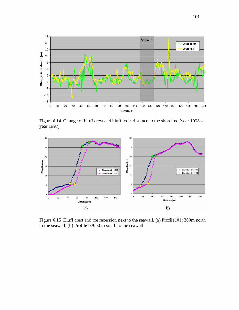
101
Figure 6.14 Change of bluff crest and bluff toe’s distance to the shoreline (year 1998 – year 1997)
Figure 6.15 Bluff crest and toe recession next to the seawall. (a) Profile101: 200m north to the seawall; (b) Profile139: 50m south to the seawall

102
Figure 6.16 Change of bluff crest and bluff toe’s elevation (year 1998 – year 1997)
Along the shoreline, the bluff volume change range from an accretion of 3.6 m3
per meter of shoreline, which is small enough to be considered within error threshold, to
erosion up to 468 m3 per meter of shoreline (Figure 6.17). The total volume loss is about
20910 m3.Given the limitation of topographic LiDAR system in terms of its water
penetration ability, the volume change of the beach portion is only determined above the
monthly mean high water level in April 1998. Within this area, the total beach volume
loss is about 13518 m3, with much less variation along shore than the bluff volume
change. The beach volume loss is mainly caused by the seasonal beach change, when
sand goes offshore in the winter, but there is still some permanent loss to the offshore.

103
Figure 6.17 Change in bluff and beach volume (year 1998 – year 1997)
6.2 A case study for object-based morphological and volumetric change analysis
The object-based coastal morphological and volumetric change analysis method is
applied to a case study area located at Assateague Island, Maryland, in the central
Atlantic coast of the US (Figure 6.18). Assateague Island is a barrier island built as wave
action piles up sand from the ocean floor, and has been constantly reshaped by the
currents, winds, and tides. Barrier islands are characteristic depositional coastal
landforms that are quite common all over the world, lying offshore of more than 10% of
the world’s coastlines. They are most extensive along the east coast of the US, extending
from New England down the Atlantic Coast, and south to the Gulf of Mexico.

104
Figure 6.18 The geographical settings of Whittington Point of Assateague Island, Maryland
6.2.1 LiDAR data preprocessing
The analysis on morphological and volumetric change is performed based on two
successive LiDAR surveys – the first survey was conducted on September 15th, 1997,
and the second was on Septmber 20th, 2000. Both two LiDAR surveys were acquired by
NASA’s Airborne Topographic Mapper (ATM) LiDAR system through the
NOAA/USGS/NASA Airborne LiDAR Assessment of Coastal Erosion (ALACE)
Project. The raw LiDAR measurements have a vertical accuracy within 0.15m and a
horizontal accuracy around 0.8m. The raw LiDAR points were interpolated into Digital
Elevation Model (DEM) at 1m spatial resolution.
Two LiDAR DEMs were projected to the UTM (zone 18) coordinate system and
horizontally referenced to North American Datum of 1983 (NAD83). The vertical datum
is North American Vertical Datum of 1988 (NAVD88). The overlapping areas were

105
extracted from two LiDAR surveys to conduct change analysis. The hillshading images
were created for both DEMs using common gray scale to provide a three-dimensional
perspective of the topography, which could also facilitate the horizontal registration and
vertical calibration (Figure 6.19a and Figure 6.19b). The vertical calibration was
conducted by using the highway as invariant feature. After vertical adjustment, a 3× 3
median filter was applied to both 1997 and 2000 LiDAR DEMs to reduce the random
errors.
6.2.2 Morphological and volumetric change analysis
The elevation change grid was created by subtracting the 1997 LiDAR DEM from the
2000 LiDAR DEM as in Equation (6.2):
19972000ijijij zzz −=∆ (6.2)
where 2000ijz and 1997
ijz are the elevation measurements for the cell (i, j) respectively at the
year 2000 and the year 1997, and ∆zij is the elevation difference for the cell (i, j).

106
Figure 6.19 LiDAR DEMs and the elevation difference grid. (a) DEM acquired in 1997; (b) DEM acquired in 2000; and (c) Cell-by-cell elevation changes during 1997-2000

107
Given a vertical accuracy of 0.15 m, the random error of elevation differences
could be as large as dσ = 0.21 m ( 15.02 × m). By setting the multiplicative factork to
2.0, the criterion of assuming that elevation change has occurred is an absolute change
value larger than dkσ = 0.42m. According to this criteria, the elevation differencing
image could be reclassified into three categories: positive change (+1), negative change
(-1), and unchanged (0).
42.042.0
42.0
42.0
,0
,1
,1
<∆<−−<∆
>∆
−=
ij
ij
ij
ij
zif
zif
zif
c (6.3)
where ijc is the morphological change code for the grid cell (i, j).
Based on the classified elevation change imagery, the positive change and
negative change objects were identified and delineated automatically (Figure 6.20). The
planimatric attributes, shape attributes, surface attributes, and volumetric attributes were
calculated for each individual object to perform a further classification.
The initial set of objects identified includes many change patches that were
induced by factors other than erosion and deposition, such as vegetation dynamics and
wave run-up. In order to focus on the sediment-induced morphological and volumetric
changes, the change patches induced by various factors were classified based on the
combination of selected attributes. For the change patches induced by vegetation
dynamics, they commonly have irregular and rough boundaries as well as many holes
and gaps, and therefore have a large fractal dimension. In addition, the changes within
vegetation patches are usually discontinuous and hence have a much larger vertical

108
standard deviation. For the change patches induced by wave run-up, they commonly
have a relatively small size. Based on these observations, three attributes were used for
the classification in this case study: fractal dimension, standard deviation of vertical
changes, and size. A set of criteria was defined to identify and remove change patches
induced by vegetation dynamics, wave run-up, and other data noise, which includes:
Fractal Dimension (D) > 1.4, or standard deviation of vertical change ( stdz∆ ) > 0.6, or
Size (A) < 190 m2. The remaining objects are considered to be changes caused by
erosion and deposition. Morphological operations were applied to smooth the remaining
erosion and deposition objects (Figure 6.21).
Figure 6.20 Negative change and positive change objects
Figure 6.21 Erosion and deposition objects after smoothing

109
For the 1.85 km coastal stretch of the case study area, totally 34 erosion objects
and 23 deposition objects were identified. All the planimetric, shape, surface, and
volumetric attributes were calculated for these objects again (Figure 6.22 and Table 6.2).
The minimum bounding rectangles and best-fit ellipse were created for each object to
generalize the shape (Figure 6.23). The summary statistics were calculated to describe
the total erosion, deposition, and net volume change in this area.
Figure 6.22 Erosion and deposition objects overlaid on the hill-shaded relief images. (a) Relief image derived from 1997 LiDAR data; (b) Relief image derived from 2000 LiDAR data

110
Table 6.2 Derived attributes values for erosion and deposition objects

111
Figure 6.23 Fitted rectangles and ellipse for erosion and deposition objects. (a) Minimum bounding rectangles; (b) Best-fit ellipses
The results indicate severe erosion and morphological change along the beach
zone. A continuous, long erosion zone (Object 563) (Figure 6.22 and Table 6.2) is
oriented along the shoreline with an azimuth angle of 62° from the true north. This
elongated erosion zone has a largest width of 35.7 m and an average erosion depth of
0.73 m. The average elevation of this zone has been reduced from 1.09 m to 0.37 m. The
total erosion volume is 10,064 m3 during 1997-2000, which is 5.448 m3
per meter of

112
shoreline stretch. Erosion processes have modified the beach from its slightly convex
downward shape (average curvature = 0.56) in 1997 to a concave upward shape (average
curvature = -0.97) in 2000. There is landward berm migration (Figure 6.22). Along the
back beach, there is a narrow deposition zone (Object 571). It was a long depression
feature in 1997 (Figure 6.22a), which was almost filled by sediment in 2000 (Figure
6.22b).This zone has a maximum width of 16.4 m and an average deposition thickness of
0.47 m. The concave surface curvature (-1.40) along the depression disappeared by 2000.
Both the erosion and deposition objects in the beach zone have elongated shapes and are
oriented parallel to the shoreline (Table 6.2).
The results also indicate significant morphological changes in the dune zone
between 1997 and 2000 (Figure 6.22), which shows a general pattern of the dune
migration to the southwest direction. Plume-like features can be observed in the south
side of many dunes in the 2000 hill-shaded relief image (Figure 6.22b). The significant
dune movement is most likely caused by the northeast winds. These winds erode and
transport sand from the dune’s upwind side and deposit on the leeward side, causing
downwind dune migration. Local redistribution of sand has produced many discrete
erosion and deposition patches in the dune zone. As expected, erosion patches occurred
on the upwind side of dunes, and deposition patches are located on the leeward side of
dunes (Figure 6.22a). The erosion patches are interspersed with deposition patches. The
position and shape of many dunes were changed considerably by erosion and deposition
processes. Compared to the elongated erosion and deposition patches in the beach, most
erosion and deposition patches in the dune zone have a more compact shape and are

113
oriented approximately perpendicular to the shoreline. The surface shape of all erosion
patches has been changed from convex to concave (Table 6.2), while the deposition
patches generally changed from concave to convex. In the dune zone, the average depth
of erosion patches reaches 0.85 m (Object 461).
For the 34 erosion objects and 23 deposition objects within the 1.85 km coastal
stretch, the average object size is 3221 m2 for erosion objects and 2378 m2 for deposition
objects. The total erosion area is 109,506 m2, and the total erosion volume is estimated
to be 66,594 m3. The total deposition area is 54,699 m2, and the total deposition volume
is estimated to be 28,223 m3. The net erosion volume is 38,371 m3. The normalized
annual net erosion volume rate is 6.9 m3 per meter of the shoreline stretch for the case
study area. The localized information could be useful for measuring, understanding and
predicting coastal morphological changes and designing future erosion control projects,
such as beach nourishments and dune management.

114
7 CONCLUSIONS
Compared to traditional ground survey and photogrammetry techniques, airborne
LiDAR remote sensing technology provides a much more cost-effective, efficient means
of collecting coastal topography information. This research has developed an analytical
framework to extract information and knowledge from the dense datasets acquired by
LiDAR surveys, which converts a large volume of raw data into meaningful and
organized information that is ready to be used in a variety of studies related to coastal
topography.
This research has developed an analytical framework for extracting coastal
morphology information. A set of algorithms and tools have been developed for
automated extraction of coastal morphological change information from LiDAR data.
The methodological contributions of this research include a set of algorithms for
automated beach profile feature extraction and change analysis, and an object-based
approach for spatial pattern analysis of morphological and volumetric change. The
algorithms and tools for automated beach profile feature extraction and change analysis
provides the cross-shore view to understand coastal morphological changes. The
algorithms and tools provide more efficient means for identifying morphological
features and deriving morphological attributes in a large geographic area. The beach
profile features and the spatial patterns of the related changes can be visualized and
analyzed along the shoreline. The representation of profiles as routes and important
features as point events also facilitates the analysis in conjunction with other GIS data

115
for exploring the causes and impacts of the morphological and volumetric changes in the
cross-shore direction.
The object-based methods for morphological and volumetric change analysis
provides an explicit object representation of erosion and deposition patches, which
makes it easy to localize attributes about individual erosion or deposition hot spots and
to analyze the spatial pattern of morphological changes. The comprehensive quantitative
information about each individual change object could facilitate the classification of
changes induced by various mechanisms, as well as support a better understanding of the
characteristics of morphological changes caused by erosion and deposition. The
representation of erosion and deposition patches as polygonal objects could also
facilitates the analysis in conjunction with other GIS data for exploring the causes and
impacts of the morphological and volumetric changes.
Both one-dimensional profile analysis and two-dimensional object-oriented
analysis algorithms have been implemented as ArcGIS extension modules. Embedding
these algorithms into ArcGIS software allows users to be able to take advantages of the
existing powerful ArcGIS functions such as data management, visualization, and spatial
analysis. The input raw LiDAR data can be directly loaded, displayed, and pre-processed
using core functions of ArcGIS and specialized extensions developed by other
organizations. The processed LiDAR datasets can be directly ingested by the volumetric
analysis module and the beach profile analysis module. The morphological change
analysis results can be immediately displayed and validated using the available ArcGIS

116
visualization functions. Also, the analysis results can be compared and integrated with
other GIS data for map composition and further numerical analysis and modeling.
LiDAR technology makes it possible to create accurate and dense datasets for
costal topography mapping and change analysis in a cost-effective manner. However, the
LiDAR surveys also suffer from some limitations. For topographic LiDAR systems, the
topography mapping in the near-shore zone is limited by its capability of penetrating
water. In terms of temporal scale, a complete understanding of the changing coastal
morphology may require more frequent surveys such as monthly or quarterly surveys
spanning all seasons. The traditional ground survey approach is able to measure the
beach up to the wading depth of the near-shore zone. It offers more flexibility in the
choice of appropriate survey time. In this sense, the traditional techniques for coastal
topography survey are still indispensable to validate, calibrate, and supplement LiDAR
data. This research focuses on the methodology for characterizing and analyzing the
coastal morphological changes based on airborne LiDAR data. By supplementing the
LiDAR datasets with other data sources, the methodology developed in this research
could be used to support the change analysis at various temporal scales, such as storm-
related changes, seasonal variations, and the long-terms changes caused by sea level rise.
The visual interpretation and automated algorithms for beach profile analysis are
complementary. The automated profile analysis algorithms are helpful in extracting
information over a large geographic area and locating the area of interests, but visual
interpretation is essential for determining reasonable thresholds, validating and adjusting
the results from algorithms. In the future, based on the vector representation of cross-

117
shore morphological features and properties, other ancillary data sources could be
incorporated to perform analysis such as conducting coastal classification, evaluating
storm hazard vulnerability, as well as evaluating the impacts of human interventions on
coastal morphology changes.
The pixel-based and object-based representations of elevation change patches are
also complementary. The pixel-based representation provides spatially distributed
information of erosion and deposition. The object-based representation is helpful in
locating hot spots and classifying the change patches, but a detailed analysis within each
erosion and deposition patches is based on the pixel-based elevation change information.
In the future, other ancillary data sources such as multispectral remote sensing imagery
could be incorporated to derive the thematic attributes of discrete change patches
(object). This will be useful for achieving a better classification of change patches
induced by various mechanisms and for gaining a better understanding of the causes and
impacts of coastal morphological changes.

118
REFERENCES
Abramowitz, M., and I. A. Stegun. 1964. Handbook of mathematical functions with formulas, graphs, and mathematical tables. Washington, DC: U.S. National Bureau of Standards. Batten, B. K., and N. C. Kraus. 2005. Regional Morphology Analysis Package (BMAP), Part2: Users guide and tutorial. Vicksburg, MS: U.S. Army Engineer Research and Development Center, Coastal and Hydraulics Laboratory. Brennan, P., and M. Harlow. 2002. Linear referencing in ArcGIS. Redlands, CA: Environmental Systems Research Institute (ESRI). Brock, J. C., W. B. Krabill, and A. H. Sallenger Jr. 2004. Barrier island morphodynamic classification based on LiDAR metrics for north Assateague Island, Maryland. Journal of Coastal Research 20 (2):498-509. Burrough, P. A. 1981. Fractal dimension of landscape and other environmental data. Nature 294:240-242. CCSR. 2006. Mapping the future world population. http://ccsr.columbia.edu/population/map/ (last accessed 31 August 2008). Chaudhuri, D., and A. Samal. 2007. A simple method for fitting of bounding rectangle to closed regions. Pattern Recognition 40 (7):1981-1989. Cooper, N. J., D. J. Leggett, and J. P. Lowe. 2000. Beach-profile measurement, theory and analysis: Practical guidance and applied case studies. Water and Environment Journal 14 (2):79-88. Crossett, K. M., T. J. Culliton, P. C. Wiley, and T. R. Goodspeed. 2004. Population trends along the coastal United States: 1980-2008. Washington, DC: National Oceanographic and Atmospheric Administration. Davis, J. C. 2002. Statistics and data analysis in geology, 3rd edition. New York: John Wiley & Sons, Inc. Elko, N. A., A. H. Sallenger Jr, K. Guy, H. F. Stockdon, and K. L. M. Morgan. 2002. Barrier island elevations relevant to potential storm impacts: 1. Techniques. USGS Open File Report 02-287. Washington, DC: U.S. Geological Survey.

119
Finkl, C. W., L. Benedet, and J. L. Andrews. 2005. Interpretation of seabed geomorphology based on spatial analysis of high-density airborne laser bathymetry. Journal of Coastal Research 21 (3):501-514. Flusser, J., and T. Suk. 1993. Pattern recognition by affine moment invariants. Pattern Recognition 26 (1):167-174. Foroutan-pour, K., P. Cutilleul, and D. L. Smith. 1999. Advances in the implementation of the box-counting method of fractal dimension estimation. Applied Mathematics and Computation 105:195-210. Gares, P. A., Y. Wang, and S. A. White. 2006. Using LiDAR to monitor a beach nourishment project at Wrightsville Beach, North Carolina, USA. Journal of Coastal Research 22 (5):1206-1219. Graham, D., M. Sault, and C. Bailey. 2003. National ocean service shoreline: Past, present, and future. Journal of Coastal Research 38:14-32. Halcrow.2008. SANDS – Managing and understanding coastal data. http://www.halcrow.com/sands/default.asp (last accessed 5 October 2008) Hapke, C. J., D. Reid, B. M. Richmond, P. Ruggiero, and J. List. 2006. National assessment of shoreline change, Part 3: Historical shoreline change and associated coastal land lost along sandy shorelines of the California coast. USGS Open File Report 2006-1219. Washington, DC: U.S. Geological Survey. Judge, E. K., M. F. Overton, and J. S. Fisher. 2003. Vulnerability indicators for coastal dunes. Journal of Waterway, Port, Coastal and Ocean Engineering 129 (6):270-278. Lindeberg, T. 1994. Scale-space theory: A basic tool for analysing structures at different scales. Journal of Applied Statistics 21 (2):224-270. Liu, H., and K. Jezek. 2004. Automated extraction of coastline from satellite imagery by integrating Canny edge detector and locally adaptive thresholding method. International Journal of Remote Sensing 25 (5):937-958. Mandelbrot, B. B. 1983. The fractal geometry of nature. New York: W.H.Freeman and Company. Mason, D. C., C. Gurney, and M. Kennett. 2000. Beach topography mapping - A comparison of techniques. Journal of Coastal Conservation 6:113-124. Meredith, A. W., D. Eslinger, and D. Aurin. 1999. An evaluation of hurricane-induced erosion along the North Carolina coast using airborne LiDAR surveys. NOAA Coastal

120
Service Center Technical Report NOAA/CSC/99031-PUB/001.Washington, DC: National Oceanographic and Atmospheric Administration. Morang, A., and L. E. Parson. 2002. Coastal Engineering Manual, Part IV - Chapter 1: Coastal terminology and geologic environments. Coastal Engineering Manual 1110-2-1100. Washington, DC: U.S. Army Coastal Engineering Research Center. Mulchrone, K. F., and K. R. Choudhury. 2004. Fitting an ellipse to an arbitrary shape: Implications for strain analysis. Journal of Structural Geology 26 (1):143-153. NOAA. 2008. Remote sensing for coastal management. http://www.csc.noaa.gov/crs/rs_apps/sensors/lidar.htm (last accessed 30 September 2008). Robertson, W., K. Zhang, and D. Whitman. 2007. Hurricane-induced beach change derived from airborne laser measurements near Panama City, Florida. Marine Geology 237:191-205. Rosin, P. L. 1993. Ellipse fitting by accumulating five points fits. Pattern Recognition Letters 14 (8):661-669. Sallenger, A. H. 2000. Storm impact scale for barrier islands. Journal of Coastal Research 16 (3):890-895. Sallenger, A. W., W. Krabill, R. Swift, J. Brock, J. List, M. Hansen, R. A. Holman, S. Manizade, J. Sontag, A. Meredith, K. Morgan, J. K. Yunkel, E. Frederick, and H. Stockdon. 2003. Evaluation of airborne scanning LiDAR for coastal change applications. Journal of Coastal Research 19 (1):125-133. Schwartz, M. L. 2005. Encyclopedia of coastal science. Dordrecht, The Netherlands: Springer. Shrestha, R. L., W. E. Carter, M. Sartori, B. J. Luzum, and K. C. Slatton. 2005. Airborne Laser Swath Mapping: Quantifying changes in sandy beaches over time scales of weeks to years. ISPRS Journal of Photogrammetry and Remote Sensing 59 (4):222-232. Sonka, M., V. Hlavac, and R. Boyla. 1999. Image processing, analysis, and machine vision, 2nd edition. Pacific Grove, CA: Brooks/Cole Publishing Company. Stockdon, H. F., A. H. Sallenger Jr, R. A. Holman, and P. A. Howd. 2007. A simple model for the spatially-variable coastal response to hurricanes. Marine Geology 238:1-20.

121
Suesse, H., and K. Voss. 2001. A new efficient algorithm for fitting of rectangles and squares. Proceedings of IEEE International Conference on Image Processing 2:809-812. Teague, M. R. 1980. Image analysis via the general theory of moments. Journal of the Optical Society of America 70 (8):920-930. Thornton, E. B., A. Sallenger, J. C. Sesto, L. Egley, T. McGee, and R. Parsons. 2006. Sand mining impacts on long-term dune erosion in southern Monterey Bay. Marine Geology 226:45-58. USGS. 2008. Storm-impact scale: First line of defense. http://coastal.er.usgs.gov/hurricanes/impact-scale/measuringdhigh.html (last accessed 5 November 2008). Veri-Tech. 2006. CEDAS 4.01. http://www.veritechinc.net/products/cedas/ (last accessed 2 October 2008). White, S. A., and Y. Wang. 2003. Utilizing DEMs derived from LiDAR data to analyze morphologic change in the North Carolina coastline. Remote Sensing of Environment 85 (1):39-47. Wise, R. A. 1995. Beach Morphology Analysis Package (BMAP), Version1. Vicksburg, MS: U.S. Army Engineer Research and Development Center, Coastal and Hydraulics Laboratory. Witkin, A. P. 1983. Scale-space filtering. Proceedings of International Joint Conference on Artificial Intelligence 2:1019-1022. Woolard, J. W., and J. D. Colby. 2002. Spatial characterization, resolution, and volumetric change of coastal dunes using airborne LiDAR: Cape Hatteras, North Carolina. Geomorphology 48:269-287. Zhang, K., D. Whitman, S. Leatherman, and W. Robertson. 2005. Quantification of beach changes caused by Hurricane Floyd along Florida's Atlantic coast using airborne laser surveys. Journal of Coastal Research 21 (1):123-134.

122
VITA
Name: Yige Gao Address: Department of Geography, Texas A&M University Room 810, Eller O&M Building, College Station, Texas 77843-3147 Email address: [email protected] Education: B.S., Geographical Information System, Peking University, China, 2005
B.S. (Double degree), Mathematics and Applied Mathematics, Peking University, China, 2005
M.S., Geography, Texas A&M University, 2009