LOCALIZATION IN LARGE-SCALE WIRELESS

SENSOR NETWORKS

TECHNICAL REPORT 2014-617

Yaser Al Mtawa, Hossam Hassanein, and Nidal Nasser { yalmtawa, hossam} @cs.queensu.ca, nnasser@alfaisal.edu

Telecommunications Research Lab (TRL) School of Computing, Queen’s University

Kingston, Ontario, Canada K7L 3N6

November 2013

©2013 Yaser Al Mtawa, Hossam Hassanein, and Nidal Nasser

i

Abstract

Localization in Wireless Sensor Networks (WSNs) has attracted much research recently.

The interest in this field is expected to proliferate since localization in WSNs is the corner stone of many applications in areas such as: smart buildings, smart vehicles, wildlife and environmental monitoring, military, health care, and merchandise tracking. The rapid growth of the number of sensors that have heterogeneous wireless technologies deployed over vast areas poses many challenges to localization systems: robustness, scalability, accuracy, energy consumption, and interoperability. Firstly, in this paper, an overview of the advantages and the limitations of various localization techniques will be provided; these localization schemes and systems will be classified into either range-based or range-free techniques. Secondly, the main focus of this paper is to overview the localization aspects in large-scale WSNs (LS-WSNs); then to analyze and evaluate qualitatively some of the existing schemes against the following metrics: accuracy, energy efficiency, scalability, resilience, and cost efficiency. Open problems for future work are also presented.

ii

Table of Contents

Abstract ....................................................................................................................................................... i

List of Acronyms ..................................................................................................................................... iv

1 Introduction........................................................................................................................................ 1

1.1 Motivation for Localization in Wireless Sensor Networks ............................................. 1

1.2 Objective of this Paper .................................................................................................... 1

1.3 Paper Organization .......................................................................................................... 2

2 Wireless Sensor Networks ............................................................................................................... 3

2.1 Background and Definition ............................................................................................. 3

2.2 Communication in WSNs ................................................................................................ 4

2.3 Constraints and Challenges ............................................................................................. 4

3 Localization in WSNs ...................................................................................................................... 6

3.1 Detailed Overview ........................................................................................................... 6

3.2 Existing Localization Approaches .................................................................................. 6

3.2.1 Single-hop vs. Multi-hop Localization .................................................................... 7

3.3 Range-based Localization in WSNs ................................................................................ 7

3.3.1 Measuring Phase ...................................................................................................... 7

3.3.2 Positioning Phase ..................................................................................................... 9

3.3.3 Summary of Localization in Range-based Systems ............................................... 12

3.4 Range-free Localization in WSNs ................................................................................. 13

3.4.1 Connectivity-based Technique ............................................................................... 13

3.4.2 Fingerprint-based Technique ................................................................................. 13

3.4.3 Summary of Localization in Range-free Systems ................................................. 13

4 Localization in LS-WSNs: Characteristics and Requirements ................................................. 15

4.1 An Overview ................................................................................................................. 15

4.2 Characteristics and Requirements ................................................................................. 15

5 Localization in Large-Scale WSNs .............................................................................................. 17

5.1 Challenges of Evaluation the Localization Systems ..................................................... 17

5.2 Performance Metrics ..................................................................................................... 19

5.3 Classification of Localization Schemes and Systems ................................................... 21

5.3.1 Range-based Localization Systems ........................................................................ 22

5.3.2 Range-free Systems ............................................................................................... 27

iii

5.4 Observations and Further Discussions .......................................................................... 35

6 Summary and Open Research Problems ...................................................................................... 37

6.1 Summary ....................................................................................................................... 37

6.2 Open Research Problems .............................................................................................. 37

References ................................................................................................................................................ 38

iv

List of Acronyms

A2L Angle to Landmark

ADC Analogue to Digital Convertor

ANR Anchor to Node range Ratio

AoA Angle of Arrival

APIT Approximate Point in Triangulation

APS Ad Hoc Positioning System

APS-AoA Ad Hoc Positioning System Using Angle of Arrival

BS(s) Base Station(s)

Bluetooth Universal short range radio connectivity

DV Distance Vector

DV-hop Distance Vector based on hops

GPS Global Positioning System

HA-A2L High Accuracy localization based on Angle to Landmark

IR Infra-Red

LANDMARC Location Identification based on Dynamic Active RFID Calibration

LoS Line of Sight

LS-WSN(s) Large-Scale Wireless Sensor Network(s)

MBAL Mobile Beacon-Assisted Localization

NLoS Non-Line of Sight

PIT Point in Triangulation

RF Radio Frequency

RFID Radio Frequency Identification

RSS Received Signal Strength

RSSI Received Signal Strength Indicator

SN(s) Sensor Node(s)

SS Signal Strength

TDoA Time Difference of Arrival

ToA Time of Arrival

UWB Ultra Wide Band

Wi‐Fi Popular technology for wireless local area networking

WLAN Wireless Local Area Network

WSN(s) Wireless Sensor Network(s)

ZigBee® a low‐cost, low‐power wireless connectivity standard

1

1 Introduction

Wireless Sensor Networks (WSNs) have been used in many fields: smart buildings, smart vehicles, health care, environmental studies, security, tracking objects, and agriculture [1-4]. For example [4], in environmental monitoring, WSNs can be used to continuously monitor drinking water for contaminants. In military applications thermal sensors can be mounted on missiles to track and then hit the target. In the healthcare domain, patients and assets can be tagged by sensors for tracking and efficient locating. Next, the motivation behind the localization in WSNs, the objective of this paper and its organization will be presented.

1.1 Motivation for Localization in Wireless Sensor Networks In many sensor-based applications such as wildfire monitoring, it is meaningless to not

know the location from where the measurement and sensed data are obtained. The process that enables the unknown (blind) sensor node (SN) to know its (estimated) location in the physical world is known as localization [5-7]. Localization in WSNs is, usually, accomplished by using techniques to estimate the location of the unknown sensor nodes (SNs) by utilizing the availability of pre-determined locations of a few specific nodes called anchors (landmarks). The anchor is usually more powerful than the other sensors in terms of processing, communication, and energy. In order to know its position, anchors are equipped with a global positioning system (GPS) [8] or placed in known locations. The applications either require fine-grain accuracy of localization or coarse-grain accuracy of localization. In the former, global coordinates are used to know the physical coordinates of the SNs. In the latter, local coordinates are enough to locate the sensor. For example, it is enough to know that the patient is in specific room in the hospital; the anchor’s coordinates, in this case, are used as a local base that all sensors are relative to. In other words, the location of the unknown SNs needs to be known by utilizing the anchor’s coordinates using localization techniques [9, 10]. In other applications where no anchors are deployed and yet relative locations are required for sensors [11], e.g. routing in WSNs, sensors are using inter-sensor measurements as a self-organizing technique to build a local map of relative positions of the sensors. Later, if such sensors require knowing their global coordinates, operations like reflections, rotations, and translation are applied providing that at least one of these sensors knows its physical position [12, 13]. There are many localization schemes and systems designed for WSNs, but none are standardized yet with the exception of GPS for outdoor use. The proliferation of localization applications of WSNs utilizing tens of thousands of sensors and too many heterogeneous technologies prompts research toward management of large-scale and heterogeneous localization systems.

1.2 Objective of this Paper Currently there is no standard for indoor localization [14-16] and research is still in

progress for outdoor localization [17-20]. The localization problem is more pronounced in large scale WSNs due to the critical challenges of scalability [21], robustness [17, 22], heterogeneity, and security [23, 24] as a consequence of the explosive growth of a number of devices with different technologies being spread over a large terrain.

In this paper, we address the problem of localization in large-scale WSNs (LS-WSNs).

We first categorize localization schemes and systems into either range-based or range-free

2

according to the technique used. The range-based schemes and systems are either distance-based which rely on Time of Arrival (ToA), Time Difference of Arrival (TDoA), Received Signal Strength Indicator (RSSI) or angle-based which relies on Angle of Arrival (AoA). The range-free schemes and systems are either connectivity-based or fingerprint-based1. The best environment to use the scheme (indoor, or outdoor), type of anchors used (static, or mobile), and the type of hop localization (single-hop, or multi-hop) will also be determined. Then we analyze and evaluate these systems qualitatively according to specific metrics. The following are the metrics that will be used to compare between the existing schemes and systems: 1) Accuracy, representing the average Euclidean distance between the exact location and the estimated location of the sensor, 2) Energy Efficiency, managing the battery power required by the SN for sensing, processing, and transmitting data, 3) Scalability, reserving the effectiveness of the localization functionality when the domain of positioning becomes larger [21, 25], 4) Resilience, measuring the ability of the system to recover from the effects of faults and maintains acceptable level of service, and 5) Cost Efficiency, managing the overhead communication, any additional hardware, time and effort taken during the deployment, i.e. the lower the cost of the system, the better its chance to work well in LS-WSNs.

1.3 Paper Organization The remaining of this paper is arranged as follows. Section 2 overviews WSNs, the

background, constraints and challenges facing WSNs. Examples of applications that clarify the importance of WSNs in our daily life will also be mentioned. Section 3 is dedicated to cover a detailed overview of localization in WSNs, possible approaches to deal with localization in WSNs such as range-based and range-free. It covers also the phases of range-based localization in single-hop WSNs, namely the measuring phase, and the positioning phase. Range-free localization in WSNs will also be studied in Section 3. Characteristics and requirements of LS-WSNs will be fully studied in Section 4. Next, Section 5 will be dedicated to study challenges of evaluation localization schemes and systems, classifying the current localizations schemes as range-based or range-free schemes, evaluating the performance of these classified schemes against suitable metrics which defined based on the requirements of localization schemes in LS-WSNs. The schemes will be evaluated qualitatively based on satisfying the features/requirements of each metric. Next, observations and further discussions will also be presented. Finally, we conclude with Section 6 in which summary and open research problems are presented.

1 A specific location spot is identified by a set of features/fingerprints of the sensed signal.

3

2 Wireless Sensor Networks

In this section, an overview of the background of Wireless Sensor Networks (WSNs) will be presented. We also address the constraints and challenges that are facing such networks. Furthermore, we show the importance of WSNs by presenting examples of applications from our daily life.

2.1 Background and Definition A WSN is composed of sensor nodes (SNs) which have sensing functionalities to

monitor physical properties such as pressure, humidity, and temperature, as well as moving objects. Each sensor has a small processor, a battery as a power supply, memory, and a short-range wireless transceiver [26]. The sensed information normally is propagated towards the base station (BS) using intermediate nodes in order to view the whole picture of the monitored region/object under tracking to the user [2]. Figure 1 shows the flow of sensed data starting from the SNs until reaching the end user. WSNs have distinguishing features that are different from the traditional Ad hoc networks. These features are [27]: • Sensors are densely deployed and cooperate to monitor detected and sensed events. • Sensors are prone to failure. • The topology of WSNs changes frequently due to signal attenuation and sensor failure. • WSNs usually use broadcast communication paradigm, where traditional Ad hoc networks

use peer-to-peer communication. • Sensor nodes (SNs) are limited in resources such as power, processing capabilities, and

memory. • SNs may not have global identification due to large overhead and sensor numbers. • WSNs are oriented to detect and/or estimate some events (not just provide communication

as in Ad hoc networks). In this regard, data aggregation can be improved by using data fusion from multiple sensors. The cluster head technique can be used to achieve this fusion method. However, this will impose a constraint on the WSNs architecture.

Base Station

Sensor node

User

Internet

Figure 1. Example of how WSN works.

4

2.2 Communication in WSNs There are two kinds of communication in WSNs: single-hop or multi-hop [28]. In the

former, the network has a star form as shown in Figure 2(a), where the BS can communicate directly with any SN in the network. However, it is not always true that each SN has direct communication with BS (i.e. single-hop communication) especially in undeterministic deployment of thousands of sensors in a vast geographical region. Even in the deterministic scenario, having single-hop communication requires denser deployments for BSs due to the short communication range of SNs causing the cost to be very high. The disadvantages of single-hop communication have been overcome by multi-hop communication. The multi-hop communication has a form of mesh network as shown in Figure 2(b), and the communication between sensors and far-off BSs occurs via multiple intermediate hops. The SN is not only transmitting its own data, but it acts as a relay for other nodes, collaborating to propagate the data towards the BS. The existence of many paths to deliver the same data to BS poses a routing problem to find the best possible path to propagate the data and eliminate the redundancy of transmitted data. It should be mentioned here that even multi-hop communication has limitations related to energy consumption. The more relaying data transmitted through a sensor, the more energy consumption for that sensor will be.

Figure 2. (a) Single-hop (b) Multi-hop communication in WSNs.

2.3 Constraints and Challenges Technological advancements have resulted in the development of inexpensive and low-

power wireless micro-sensor networks. Figure 3 shows the components of the sensor node. Each sensor consists of four main components: power unit which is usually a small battery, sensing unit which made up of the sensor and the analogue to digital convertor (ADC), processing unit which has two subunits: the processor and the memory, and communication unit which is the antenna in a wireless sensor that keeps the sensor connected to the network. These units have severe resource limitations especially in their power supply, processing power, memory, and bandwidth [26]. Additional components can be added to the sensor’s structure according to the application needs. For example, the localization system component (in dashed box) can be added to meet the localization requirements of some applications.

WSNs usually use multi-hop communication to deliver data from sensors to BSs. This will impose a routing problem [29]. An efficient routing protocol for WSNs should consider the tight budget of resources in such networks. Energy can be saved if WSNs rely on distributed

BS

Sensor

(b)

BS

Sensor

(a)

5

communication to arrange the processing power among all nodes not only on a specific node(s) as in the cluster head, and coordinators in the traditional Ad hoc networks. WSNs should be able to function normally with an acceptable overhead. Therefore, the protocols used in WSNs should be light in power consumption and not require a long running time (i.e. low computational complexity); otherwise, the battery will be depleted quickly, and the network will start disconnecting [30]. Security is also a major issue here in the sense that the network should be robust against security attacks and that the data integrity should be preserved. These constraints: limited power supplies, processing power, memory, and bandwidth along with the topology changes of WSNs pose serious problems related to data accuracy, and energy efficiency which affects the connectivity and consequently the lifetime of the entire network, which then causes the WSN to become dysfunctional.

Sensing Unit Processing Unit Communication Unit

Figure 3. Sensor node and its components.

6

3 Localization in WSNs

This section covers a detailed overview of localization in WSNs, possible approaches to deal with localization in WSNs such as range-based and range-free. Furthermore, we also address the phases of range-based localization in single-hop WSNs. We deal specifically with the measuring phase and positioning phase. Measuring phase uses either distance-based or angle-based techniques; while positioning phase derives the SN’s location by using the measuring estimates generated from the first phase, and then applies methods such as lateration, multilateration, and angulation. Range-free localization which uses methods such as connectivity and fingerprint to estimate the locations of SNs in WSNs will also be covered.

3.1 Detailed Overview Many of the aforementioned applications in WSNs require knowledge of the exact

positions of sensors and a node in a WSN has to be aware of its location in the physical world. The process of determining the location of the sensor is called localization. Localization of sensors can be achieved by one of the following ways [6, 31]: 1) manually configuring a location into each node, which may not practical for many uses such as a harsh environment where monitoring inherently depends on undeterministic deployment. Furthermore, it is impractical in the case of mobile sensors; 2) equipping every node with a Global Positioning System (GPS) receiver. This, however, increases the cost of the sensor. In fact, the current capabilities and resources (like processing and power) of most sensors cannot fit a GPS receiver. Another deployment limitation is that the GPS does not work indoors properly [6] and 3) designing algorithms to locate the sensors [32].

3.2 Existing Localization Approaches Localization techniques in the literature are classified in many ways depending on a set

of features related to the deployment environment (indoor, or outdoor), how the scheme is executed (centralized, or distributed), mobility of anchors used (static, or mobile), the way of communication between nodes of the network (single-hop or multi-hop) as shown in the next subsection, [28]. In this paper, we are providing a new classification that depends on range-based versus range-free approaches as shown in Figure 4. Further explanation for these two approaches will be presented in sub-Sections 3.3 and 3.4.

Figure 4. Special classification of localization schemes.

7

3.2.1 Single-hop vs. Multi-hop Localization Most localization schemes and systems depend on the communication between sensors

nodes and anchors. Communication in WSNs is either single-hop or multi-hop communication as illustrated in Section 2.2. Single-hop localization uses single-hop communication between the SNs and anchors; multi-hop localization uses multi-hop communication. In addition to what was mentioned in Section 2.2, multi-hop localization suffers from error propagation where the error accumulates as the hopping is continuous [28]. That is why range-based schemes and systems, that seek good accuracy, use single-hop localization. The range-free localization schemes can be either single-hop or multi-hop [33]. Connectivity-based systems usually use multi-hop localization such as in DV-hop scheme [34], while other range-free fingerprint systems are inherently single-hop systems such as RADAR [35] or LANDMARC [36] as explained in Section 5.

3.3 Range-based Localization in WSNs In range-based techniques, two main phases are usually involved to localize SNs in

WSNs [28, 37]: the measurement estimation phase, and the positioning derivation phase. We address first the measuring phase and its related issues.

3.3.1 Measuring Phase This phase is concerned with utilizing the exchanged data between the SNs and anchors

to estimate the distances or angles according to the technology used. For example, Time of Arrival (ToA), Time Difference of Arrival (TDoA) [38], and Received Signal Strength Indicator (RSSI) are used for distance estimates, where Angle of Arrival (AoA) is used to estimate the angle between the sensor and the anchor. The next sub-section deals with the techniques that are usually used to estimate the distance measurements.

3.3.1.1 Distance-based techniques In the distance estimation phase, a node merely estimates its distance to other nodes in its

vicinity. Distance estimation between two SNs (sender and receiver) is estimated by using measurements taken from some characteristics of the signals exchanged between these sensors, including [5, 32, 39]: signal speed, the elapsed time between sending and receiving the signal (time of flight), signal orientation, or signal strengths. The distance estimation phase typically utilizes one or more of the following techniques:

1) Time of Arrival (ToA) [40]: capitalizing on the relationship between signal speed, time of flight, and distance. This technique is widely used due to its simplicity since there is no need for additional hardware. However, it faces a difficulty in accurate calculation of the propagation time due to the high signal speed comparing to the distance2. Also, it requires highly synchronized clocks between the sender and the receiver.

2) Time Difference of Arrival (TDoA) [38]: following the same concept of ToA, however, it uses two different types of signals such as radio and acoustic. There is no need to synchronize the clocks of the two sensors. TDoA requires additional hardware viz. microphones and speakers.

3) Received Signal Strength Indicator (RSSI) [41]: depending on the power of the transmission signal and the strength of the received signal, these values are compared to a specific model, such as the path loss model and then derives the estimated distance. This

2 The speed of radio signal, in a vacuum, is 3x108 metresper second. e.g., 30 ns are only required to travel distance of 10m.

8

technique does not require any additional overhead since it is taking place anyway between the sender and the receiver. However, it suffers from multipath fading, and shadowing.

The following sub-Section addresses the technique to estimate the angle between the sender and the receiver nodes in WSNs.

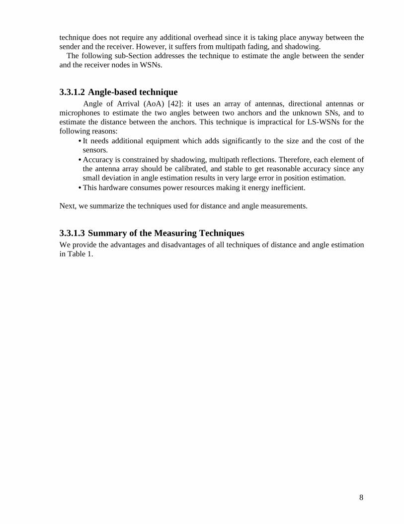
3.3.1.2 Angle-based technique Angle of Arrival (AoA) [42]: it uses an array of antennas, directional antennas or

microphones to estimate the two angles between two anchors and the unknown SNs, and to estimate the distance between the anchors. This technique is impractical for LS-WSNs for the following reasons:

• It needs additional equipment which adds significantly to the size and the cost of the sensors.

• Accuracy is constrained by shadowing, multipath reflections. Therefore, each element of the antenna array should be calibrated, and stable to get reasonable accuracy since any small deviation in angle estimation results in very large error in position estimation.

• This hardware consumes power resources making it energy inefficient.

Next, we summarize the techniques used for distance and angle measurements.

3.3.1.3 Summary of the Measuring Techniques We provide the advantages and disadvantages of all techniques of distance and angle estimation in Table 1.

9

Table 1. Advantages and disadvantages of the range-based localization techniques Localization Technique Advantages Disadvantages

ToA

� No need for additional hardware � low cost

� Requires highly accurate synchronization of the sender and receiver clocks. � Adding to the cost and complexity of a sensor network.

� Difficulty in accurately measuring the time of the flight.

TDoA

� No need for synchronization of the clocks of the sender and receiver.

� Can obtain very accurate measurements.

� Requires additional hardware like a microphone and speaker for the given example.

RSSI

� No additional hardware is necessary.

� Distance estimates can even be derived without additional overhead from communication that is taking place anyway.

� RSSI values are not constant but can heavily oscillate, even when sender and receiver do not move (fast fading, mobility of the environment, and presence of obstacles in combination with multipath fading).

AoA

� No need for synchronization of the sender and receiver clocks.

� The accuracy of AoA measurements is limited by the directivity of the antenna, by shadowing and by multipath reflections.

� Additional hardware can obtain more accuracy, but add significantly to the size and cost of SNs.

� It is not advised to be used in large-scale WSNs (LS-WSNs).

By completing the measuring phase of localization, we address in next sub-Sections the positioning derivation phase and its related methods.

3.3.2 Positioning Phase

In the positioning phase, the distance or angle measuring estimates collected in phase one are respectively used by lateration or angulation methods, to compute the position of the blind node [14, 43-45]. Next, we start by lateration method.

3.3.2.1 Lateration Method In general, the lateration method requires (n+1) distance measurements from the

unknown node to the anchor node to estimate the blind node’s location in (n) dimensions [46]. Tri lateration depends on three distance measurements to be calculated, then the position (in 2D) of the unknown node is the intersection coordinates of the three circles centered in the anchors with distance measurements as radii [47, 48]. Trilateration is an essential geometric method

10

which is involved in many localization systems such as GPS, as explained later in Section 5. In the following example, 1 2 3, ,and r r r are three range measurements between the unknown node,

u, and the three anchor nodes A, B, and C located at( ) ( ) ( )1 1 2 2 3 3, , , , and ,x y x y x y ,

respectively. In ideal case where no errors are imposed to the localization, the estimated position ( ), u ux y for SN u is the intersection of the three circles as shown in Figure 5.

ur1

A

r2

r3

B

C

Figure 5. Trilateration method in ideal case

The estimated position of u ( ), u ux y can be then calculated algebraically by solving the

following non-homogeneous system.

2 2 2 2 2 23 1 3 1 1 3 1 3 1 3

2 2 2 2 2 23 2 3 2 2 3 2 3 2 3

( ) ( ) ( )

( ) ( ) ( )2

u

u

x x y y x r r x x y y

x x y y y r r x x y y

− − − − − − −

− − − − − − −

=

This system of equations has the form Ax b= where 0.5A is the leftmost matrix, x is the

unknown vertical vectoru

u

x

y

, b is the rightmost vector.

Next, we address multilateration method which is similar to trilateration, but with one

difference that multilateration can use more than three anchors to estimate the location of the unknown SN.

11

3.3.2.2 Multilateration Method To avoid ambiguity and determine uniquely the location of a point in a plane using

trilateration, the three positions of the anchor nodes should be non-collinear. Furthermore, the measurement techniques such as ToA, TDoA, RSSI, AoA are biased estimators which means that there is a difference between the actual value of the distance (or angle) measurement and the estimated one. Thus, the measurements are erroneous which may result in the three corresponding circles (in trilateration method) not intersecting in a point; instead their intersection is an enclosed region as shown in Figure 6. The smaller this region is the less error affecting the localization resulting in better accuracy.

u

A

B

C

Figure 6. Trilateration method in real case

Multilateration method [25, 30] is a generalization of trilateration method and requires

more than three anchor nodes for localization. Multilateration, along with mean square error technique achieves the best estimation of the unknown vector x such that

2Ax b− is

minimum. Note that if the anchor is mobile, then more than three non-collinear positions for this anchor node are required for multilateration.

In next sub-Section, we deal with angulation method that utilizes the angle estimation to derive the position of the SN.

3.3.2.3 Angulation Method Angulation utilizes the AoA measurements to apply the trigonometric fact that if two

angles and the side between them are known then the position of the third point can be calculated as the intersection of the other remaining sides [7, 30, 37, 49]. For example, in Figure 7, A and B are two anchor nodes with known positions; while u is unknown sensor node. 1θ

and 2θ are the measurements of AoA technique. The distance between A and B can be calculated; then the angulation method is applied to estimate the position of u.

12

Figure 7. AoA measurements

3.3.3 Summary of Localization in Range-based Systems

Figure 8 shows a flowchart that summarizes the localization process in single-hop range-based systems.

Figure 8. Localization process in a single-hop range-based system.

The flowchart above shows a three-phase process to localize sensors in WSNs. The first phase is the beaconing phase which is a default stage as it occurs by the spontaneous signaling and packet exchange between SNs and anchors. The second phase is the measuring phase where the distance or angle measurements are estimated by using the measuring techniques such as: ToA, TDoA, RSSI, or AoA. The output of the second phase (i.e. measurements) is entered as an input to the third phase (i.e. positioning phase) where the location is derived by using the positioning methods such as lateration or angulation.

At this point, we completed the explanation of range-based approach and its related issues. Next, we deal with range-free localization approach.

u

A (x1 , y1) B (x2 , y2)

ᶿ1 ᶿ2

13

3.4 Range-free Localization in WSNs Range-free technique provides coarse-grained localization since it does not depend on

calculating distances between the unknown objects3 (the objects to be localized) and the anchor objects (the objects with known positions); instead it estimates implicitly the ranges and then the location in a broad manner [12, 33] to overcome the drawbacks of range-based techniques (i.e. cost and energy consumption). Range-free schemes and systems can be classified to either connectivity-based or fingerprint-based. The former depends on the topology of the networks, where the latter depends on storing information of some locations (prints) for retrieving and utilizing at a later time. In both cases, the implicit estimation of the range and location is erroneous and does not fully reflect the actual distance and location. However, range-free techniques provide a cost-effective alternative to the expensive range-based techniques and, hence, they are very prominent in LS-WSNs. This class of techniques is particularly oriented to the applications that do not require high accuracy in localization.

3.4.1 Connectivity-based Technique Connectivity-based schemes depend on graph topology of the network [50]. Some

techniques such as DV-hop [34] utilize the minimum hop count (i.e. shortest path) between the unknown sensor and the anchors to estimate the distances first and then the location. Other connectivity-based techniques depend on polygons in which the vertices are anchor nodes. For example, APIT scheme [51] utilizes the triangle of three anchors and decides whether the unknown SN is inside this triangle or not. Using this information, a SN’s location can be estimated by intersecting all triangles containing this SN and then taking the centroid of this intersected region.

3.4.2 Fingerprint-based Technique Fingerprint or scene analysis depends on two phases. The first phase is constructing the

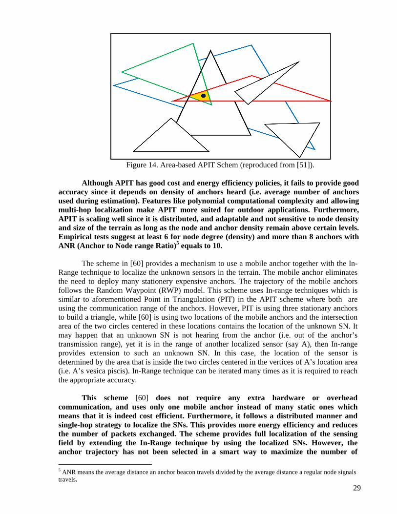
offline data base by recording RSSI at different locations with respect to different anchors from which an RF map is constructed. The second phase (i.e. online phase) matches a set of observed RSSI values with the recorded RSSI values in the database created by the offline phase. Clearly, this approach is time consuming and impractical for LS-WSNs. RADAR [35] and LANDMARC [36] are examples of such fingerprint systems as explained later in Section 5.

3.4.3 Summary of Localization in Range-free Systems Figure 9 shows a flowchart that provides the localization process in range-free systems.

3 Since an object can be equipped with sensors, then for simplicity we will use the terms node and object interchangeably.

14

Figure 9. Localization process in a range-free system.

Like Figure 8, Figure 9 shows a three-phase process to localize sensors in WSNs. The first phase is the same in both figures with a slight change in Figure 9 where mapping can be used a priori in range-free fingerprint systems. The second phase is different since range-free system has no measurement estimates; instead it approximates the distance by other means such as number of hops, ranging-in that checks whether the SN is in range or not, anchor location, or fingerprint techniques. The third phase is the positioning phase. It takes the measurement approximation as input and applies a positioning method such as: lateration, angulation, mapping, intersection, or statistical models to derive the SN’s location.

The advantages and disadvantages of the range-free schemes and systems are listed in Table 2.

Table 2. Advantages and disadvantages of the range-free localization techniques Localization Technique Advantages Disadvantages

Connectivity � No need for additional hardware

� low cost

� Provides coarse-grained localization � not accurate.

Fingerprint

� No need for additional hardware � low cost

� Provides coarse-grained localization � not accurate.

� More effort and time are needed to build the offline database. � Not practical for large-scale WSNs.

� More suitable for indoor applications.

The next section deals with characteristics and requirements of localization in LS-WSNs.

15

4 Localization in LS-WSNs: Characteristics and Requirements

In this section, we address the characteristics and requirements of localization in LS-WSNs. This characterization is an important procedure to create the performance metrics to evaluate the localization schemes and systems in LS-WSNs.

4.1 An Overview Many localization schemes have been designed to work in a centralized manner, indoor

or outdoor, with homogeneous, small numbers of (almost stationary) sensor nodes (SNs) for a particular terrain [3, 16, 25, 39]. However, in LS-WSNs, the localization scheme still has the goal (as the existing schemes) to localize the SNs with good accuracy, but LS-WSNs face new challenges such as large scale of terrain and SN numbers, dynamic changes in environment, technology used, signal traffic, and, probably, changes in positions of the SNs [33, 52].

4.2 Characteristics and Requirements

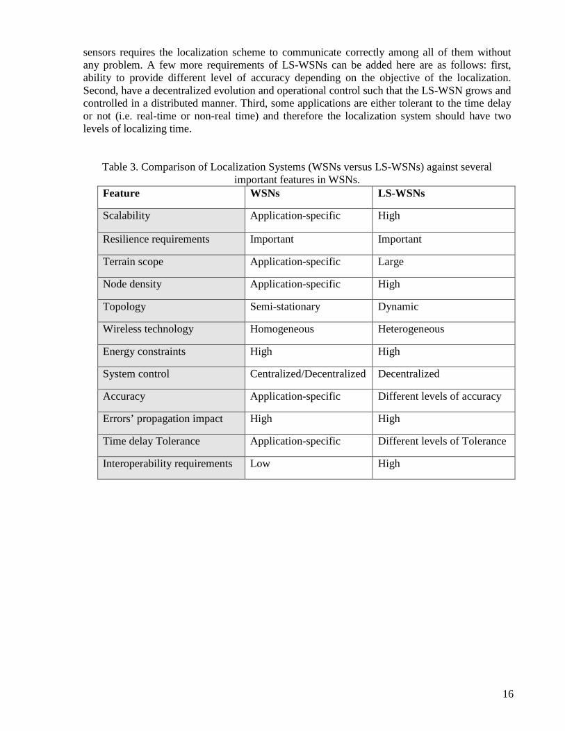
The rapid proliferation of wireless technologies speeds up the forming of LS-WSNs by making the sensors smaller and cheaper. The main characteristics of localization in LS-WSN are: heterogeneity where various wireless technologies may be used by different nodes in the network such as Wi-Fi and cellular technologies, scalability which preserves the effectiveness of the localization functionality when the domain of positioning becomes larger, cost efficiency which keeps the cost in terms of time, effort, and money within acceptable rate no matter how large the network expands, and energy efficiency which optimizes the energy consumption regardless of the technologies used. Table 3 compares between localization in WSNs versus localization in LS-WSNs against several important features. It highlights the aforementioned characteristics of LS-WSNs as the critical differences.

The requirements of localization in LS-WSNs will be discussed in details in the rest of this section. The Empirical studies [41] showed that errors increase over distance. Thus, in LS-WSNs, encountering error is a norm rather than exception and this error propagates through the network. Because of the errors are inherent to WSNs, the localization accuracy will be affected severely. To prevent this, the localization scheme should be robust enough to recover from any error. Also, people will not just be users of the system, but they may affect the overall emergent behavior of the system by being, for example, mobile users, or obstructions to the exchanged beacons. Furthermore, the localization system should be able to localize all sensors over the whole region regardless of the number of sensors and area of the region. This leads to an important issue which is that the localization scheme in LS-WSNs should rely on multi-hop and distributed communication to utilize the localization information from (at least) the local neighborhood of the unknown node and to distribute the processing power among all nodes not only on a specific node(s) like cluster head, and coordinators in the usual WSNs and Ad hoc networks. Consequently, the localization systems should be able to function properly within the constrained budget of energy, processing, and memory. In this regard, the localization system should be light in power consumption and requires short run time (i.e. low computational complexity), otherwise, the battery will be depleted quickly and the network starts disconnecting which shortens the lifespan of the network [30]. Furthermore, the different technology used by

16

sensors requires the localization scheme to communicate correctly among all of them without any problem. A few more requirements of LS-WSNs can be added here are as follows: first, ability to provide different level of accuracy depending on the objective of the localization. Second, have a decentralized evolution and operational control such that the LS-WSN grows and controlled in a distributed manner. Third, some applications are either tolerant to the time delay or not (i.e. real-time or non-real time) and therefore the localization system should have two levels of localizing time.

Table 3. Comparison of Localization Systems (WSNs versus LS-WSNs) against several important features in WSNs.

Feature WSNs LS-WSNs

Scalability Application-specific High

Resilience requirements Important Important

Terrain scope Application-specific Large

Node density Application-specific High

Topology Semi-stationary Dynamic

Wireless technology Homogeneous Heterogeneous

Energy constraints High High

System control Centralized/Decentralized Decentralized

Accuracy Application-specific Different levels of accuracy

Errors’ propagation impact High High

Time delay Tolerance Application-specific Different levels of Tolerance

Interoperability requirements Low High

17

5 Localization in Large-Scale WSNs

The performance evaluation of localization in Large-Scale Wireless Sensor Networks (LS-WSNs) faces many challenges that are related to LS-WSNs characteristics as mentioned earlier in Section 4. In this section, we address these challenges and we classify the current localization schemes and systems as range-based (e.g. distance- and angle-based schemes and systems) or range-free schemes and systems (e.g. connectivity-based and fingerprinting-based schemes and systems). Then we define special performance metrics for LS-WSNs based on the requirements of LS-WSNs schemes and systems presented in previous section. Later, we compare the classified systems against the defined metrics. The schemes will be evaluated qualitatively based on satisfying the features/requirements of each metric. Furthermore, observations and further discussions will be presented. Moreover, we select to the best fitting schemes for localization in LS-WSNs and propose further enhancement for such schemes.

5.1 Challenges of Evaluation the Localization Systems

The problems that are facing the localization systems in LS-WSNs are not different from those problems in ordinary localization systems in WSNs. However, the characteristics of LS-WSNs are prone to problematic challenges. In this section, we will address such problems and the factors behind them. Firstly, we will present the challenges in evaluating the localizations systems. Secondly, we discuss the factors behind these challenges.

The challenges are twofold: first there is no generally accepted metrics to compare the

performance of localizations systems and second, there is no generally accepted methodology to design, simulate, emulate, and deploy the localization system [53].

The factors behind these challenges are, but not limited to, the following:

1- The type of localization techniques being used in the system. The schemes differ from each other in the techniques used. The system can be range-based or proximity-based. Even in each category, there are differences. For example, the range-based uses different measurement techniques such as ToA, TDoA, RSS, or AoA. Each of these techniques has advantages and drawbacks that affect the measurement errors.

2- Involving of the anchors (beacons) in measurement estimation. Some systems use anchors, where others do not. Usually the techniques that use anchors provide more accurate localization compared to the other schemes which do not use anchors. The other issue that should be mentioned here is the type of anchors used (i.e. static or mobile). The mobile anchor [22, 54] can do the work of several static anchors and scale over a large area of terrain. So usually the mobile anchor can be more suited for LS-WSNs if its trajectory is predetermined in such a way that covers the whole terrain. On the other hand, large numbers of static anchors (according to its communication range) should be deployed to cover the whole area.

3- The type of nodes being localized (i.e. static or mobile). Usually localizing the static SN is more accurate compared to the mobile one. The reason behind this is that the mobile SN is generating more measurement error since there is always time gap (depends on the speed of the mobile SN) between the current position of the unknown mobile SN and the new position until it gets localized. This leads to degrade the accuracy of localization. Furthermore, a mobile SN is more likely to face changes in direction, obstruction, and environment like

18

wind, humidity, and sun light. All these changes affect the performance of the localization techniques.

4- The distribution of anchors and blind node in the localization area [53]. There are applications that use predetermined (i.e. deterministic) positions of each anchor and node such as grid deployment and fingerprinting (scene analysis). For example, grid distribution will affect the design and the performance of the localization system positively since each anchor will cover part of the grid and this will minimize the interference between anchors and reducing the exchanged messages. Thus, the overhead communication will be reduced, the energy power will be efficiently used, and this prolongs the life of the network. Unfortunately, this is not always the case especially in large scale WSNs where the nodes and anchors are distributed in an un-deterministic way.

5- The density of the nodes in the network (i.e. average number of neighbor SNs). If the nodes are distributed densely, then the whole network will be covered by using multi-hop beaconing. However, this will cost more in message exchange overhead and thus power consumption. The batteries of the nodes will be depleted and eventually the network starts disconnecting. Thus, the density of nodes will not help at all in scalability and robustness and hence, it is not suitable for LS-WSNs.

6- The environment where the system will be deployed (i.e. indoor or outdoor). Usually the localization systems are application-oriented. Some applications require indoor localization, where the others require outdoor. Usually the indoor systems utilize the infrastructure available inside the building such as WLAN, RFID, or IR. These systems are facing some problems like non-line of sight (NLoS), multipath, and reflection. On the other hand, outdoor localization systems may face the same problems, as in indoor environment, but with less severity. Furthermore, another problem related to environmental change can affect the performance of outdoor systems. Moreover, it is worthy here to mention that the localization systems in LS-WSNs should work indoors and outdoors and be robust against the problems mentioned above.

7- The wireless technology used in the network where the localization system is being deployed can be either homogeneous or heterogeneous. If it is the former, then this will simplify the design of localization system since the distributed localization algorithm deals with one technology only. On the other hand, if it is the latter, then this will impose an interoperability problem to handle various kinds of technology and applications used by different nodes of the network. Usually the systems are interoperable if it consists of modular components; each of which has low coupling and high cohesion. Furthermore, it should be able to interface smoothly with other applications.

8- The nature of the localization scheme (i.e. centralized or distributed). There are differences between centralized schemes and distributed schemes regarding significant features such as accuracy, computational complexity, and energy consumption [37]. The centralized algorithm is more likely to provide more accurate localization since it can be designed to get a global optimal solution; in contrary to the distributed algorithm in which there is no guarantee to get a global optimal solution even if its components reached the local optimal solution [37]. Furthermore, the centralized algorithm has higher computational complexity and energy consumption. This is a result of higher volume of messages exchanged between the nodes of the network. Therefore, the centralized localization schemes are not feasible for localization in LS-WSNs. It is worthy to mention here that error propagation is a potential problem in distributed schemes where the errors are accumulated over the multi-hop path and, hence, the SNs far away from the anchor are most likely to be less accurate in their locations.

19

5.2 Performance Metrics

In light of the general requirements of LS-WSNs outlined in the previous section, the following performance metrics along with their own requirements can be derived to evaluate and analyze the current localization schemes and systems.

a) Accuracy, representing the average Euclidean distance between the exact location and the estimated location of the sensor. In general, we seek to mitigate the effects of errors on the accuracy otherwise, the errors will be accumulated dramatically through the multi-hop path and the accuracy level will drop sharply. The accuracy of localization scheme is related to the following requirements: 1) Multi-level accuracy which indicates the ability of the system to provide fine-grained and

coarse-grained accuracy. 2) Tolerate obstructions like walls, and floors 3) Use building technology infrastructure like WLAN, IR, and UWB 4) Tolerate well in weather changes such as temperature, humidity, sun, and wind. 5) Uses medium-range to long-range communication. It should be mentioned here that if the system fulfills the requirements 2 and 3 above, then it is more likely to provide good accuracy in an indoor environment. It has good accuracy for an outdoor environment if it fulfills requirements 4 and 5.

b) Energy Efficiency, managing the battery power required by the SN for sensing, processing, and transmitting data. Efficient energy consumption prolongs the lifespan of the network. The requirements related to this metric are the following: 1) Maintain low computational complexity. The lower running time scheme the better in energy

efficiency. However, if the unknown node is mobile, then tracking this node means repeating the algorithm many times which increases the power consumption even if the algorithm itself has low time computational complexity.

2) Minimize number of messages exchanged. The scheme should avoid the overhead cost of messaging between nodes by dropping the extra useless messages. For example, it is more efficient to design a localization algorithm that drops the packets which add nothing to the localization process rather than burdening the LS-WSN with a flood of packets.

c) Scalability, reserving the effectiveness of the localization functionality when the domain of positioning becomes larger. Large-scale localization schemes should have high scalability in terms of number of SNs to be localized and the region to be covered. The scalability metric is related to the following requirements: 1) Uses decentralized algorithm that enables each node to localize itself by estimating the

measurements locally and receiving the other information from the neighbors. 2) Scale with respect to the number of nodes. The localization scheme should be able to localize

the new deployed nodes by guaranteeing the coverage of these nodes by anchors either directly or through a multi-hop route.

3) Scale with the area of the region. The scheme should be able to cover larger area than the original one by installing more static anchors or using mobile anchors.

d) Resilience, measuring the ability of the system to recover from the effects of faults and

maintains acceptable level of service. In LS-WSNs, localization scheme should be tailored for interoperability, limited resources available, and other obstructions related to the environment and terrain. The following requirements are related to this metric:

20

1) Design policies to deal with interventions. For example, if any moving objects suddenly blocks the unknown node from the anchor, in this case, the scheme should have a policy to recover from this state by rerouting the message through a multi-hop path.

2) Design policies to deal with failure. The failure can be an anchor failure to continue sending beacons to the surrounding nodes, or failure finding three nodes to estimate the position by using trilateration method. The scheme should have a refinement/maintenance phase to recover from such failures.

e) Cost Efficiency, includes the overhead communication, any additional hardware, and time and effort. This means the lower the cost of the system is, the better chance it will be applied in LS-WSNs. The requirements related to this metric are the following: 1) Maintain low overhead communication. Some systems do not consider beaconing traffic

between the SNs, increase the overhead and affect negatively the communication cost by consuming unnecessary power.

2) No additional hardware is required. Additional hardware will not only increase the size of the sensor, but the cost as well while on a LS-WSN this could raise the cost dramatically.

3) Less time and effort. In a large-scale environment, there should be less time and effort to deploy the SNs and anchors. Otherwise, the localization scheme will be impractical.

The qualitative evaluation of different metrics is based on the LS-WSNs requirements. The evaluation can be Good, Moderate, or Poor. The evaluation of localization scheme or system is Good, with respect to a specific metric, if it satisfies all the requirements corresponding to that metric. The evaluation is Moderate if it satisfies a subset of the related requirements. The localization scheme or system is Poor if satisfies none or one of the associated requirements. In light of the previous discussion about metrics and their associated requirements in localization of LS-WSNs, Table 4 represents our defined assessments to evaluate qualitatively the above metrics.

21

Table 4. The qualitative evaluation of LS-WSNs metrics and their associated requirements

5.3 Classification of Localization Schemes and Systems The tracking and localization systems, in the literature, are purpose-oriented and related

to the nature and domain of their applications. There are many ways to classify such systems based on a set of features as shown in the following scenarios:

• The way scheme is executed: centralized versus distributed. • The target environment: indoor versus outdoor. • Anchor mobility: static versus mobile. • Technology used: RFID, WLAN, UWB, or Bluetooth. • Measurement used: distance-based versus proximity-based. • Space dimensions: 2D versus 3D.

Metric System requirements (ideal case) Assessment

Good Moderate Poor

Accuracy 1) Multi-level accuracy

2) Tolerate obstructions

3) Use Building technology infrastructure

4) Tolerate well in weather change

5) Use medium- to long-range communication

1, 2, 3, 4, 5

2 and 3

(good indoor)

Or

4 and 5

(good outdoor)

Any one of the last four |none

Energy Efficiency

1) Maintain low computational complexity

2) Minimize number of message exchanged

1, 2 1|2 none

Scalability 1) Use decentralized procedure

2) Scale with respect to the number of nodes

3) Scale with the area of the region

1, 2, 3 Any two 1| none

Resilience 1) Design policies to deal with interventions

2) Design policies to deal with failure

1, 2 1 | 2 none

Cost Efficiency

1) Maintain low overhead communication

2) No additional hardware

3) Less time and efforts

1, 2, 3 1|2|3 3| none

22

This section is dedicated to review and provide a new classification for some current localization systems. The systems will be classified based on range-based versus range-free. The range-based schemes and systems will be sub-classified into: distance-based or angle-based, while the range-free schemes and systems will be sub-classified into: connectivity-based or fingerprint-based.

5.3.1 Range-based Localization Systems In range-based localization schemes, two phases are usually involved to localize SNs in

WSN: 1) measurement estimation phase; and 2) positioning derivation phase. The range-based localization system is either a distance-based system or an angle-based system. We will deal first with distance-based localization systems.

5.3.1.1 Distance-based Systems The Global Positioning System (GPS) [8] is one of the most successful and widespread

single-hop localization systems for outdoor use. It requires four satellites; three for trilateration and the fourth provides more accuracy as shown in Figure 10. Since the distances between the satellites and the localized node are huge, therefore any small clock drift results in huge localization error4. For this reason each satellite equipped with an atomic clock and the fourth satellite is used for correcting the time of the receiver node. The sensor equipped with GPS receives the RF signals from the satellites and then uses them to estimate the values of time and position. GPS uses Time of Arrival (ToA) as a measuring technique to estimate the distance measurements that are used in positioning phase to estimate the location of the node. The GPS embedded in the SN calculated the time difference (signal time of flight) between the sending time RF signals from satellites to the receiving time of these signals by SN. Then the time difference is used to measure the estimated distances to apply the trilateration method and estimate the location of the sensor with accuracy best than 10metres.

Figure 10. Four stallites are needed for accurate positioning in GPS system.

4 One millisecond of time drift would result in a localization error of nearly 300km.

23

Although GPS is a popular system and works well outdoors, it fails to work indoors

where non-line of sight (NLoS) is available. The localization in this case is centralized as each sensor node has to localize itself. If any RF signal has not been received successfully from any satellite, then the signal will be retransmitted again. Furthermore, attaching additional hardware (i.e. GPS) to SN’s structure will increase the cost in terms of money and size. Moreover, GPS failed to fulfill the filtering requirement (i.e. Energy efficiency) since the sensor’s battery will not last using GPS.

The Cricket system [55] is a TDoA-based, indoor, and single-hop localization system

which uses multimodal sensing technology by utilizing RF and ultrasound (US) together. The anchor nodes act as an active transmitter for a pair of RF signals and ultrasonic waves. The unknown SNs (Cricket nodes) receive (using listeners) these signals/waves from various anchors and apply TDoA to estimate the distance. However, due to temperature change, which severely affects the speed of ultrasonic waves, a system of distance measurement calibration is applied to provide more accurate measurements. Then the unknown sensor nodes use the calibrated distance estimates in trilateration to estimate their locations. It should be mentioned here that Cricket nodes can be either static or mobile and still the scheme is able to locate and track them successfully within approximately 11 metres away from at least three anchors required for the trilateration. The accuracy of the Cricket is within centimetres and the Cricket node costs less than $10.

The Cricket system provides good accuracy for an indoor environment. However,

this accuracy is constrained by factors such as: the availability of line of sight (LoS), limited range of approximately 11m between the anchor and the listener (the closer distance, the better accuracy), and the angles between the faces of the anchor and the listener as shown in Figure 11. In other words, special placement is needed which requires more time and effort to deploy. These constraints, also, degrade the ability of this system to be scalable despite the fact that it is decentralized. Furthermore, the Cricket system requires additional and special hardware, a transceiver for both RF and US, and this increases the cost sharply in the large-scale environment. Moreover, the authors [55] considered a simple protocol to avoid collision to save energy and reduce interference amongst nearby beacons. However, some of the nodes may not be localized due to poor signal reception, and the single-hop policy of the system will not help to localize such sensors which can be resolved by multi-hop routing to exchange the localization information locally.

Figure 11. Specific alignment of a Cricket ultrasonic transmitter (reproduced from

[55]).

24

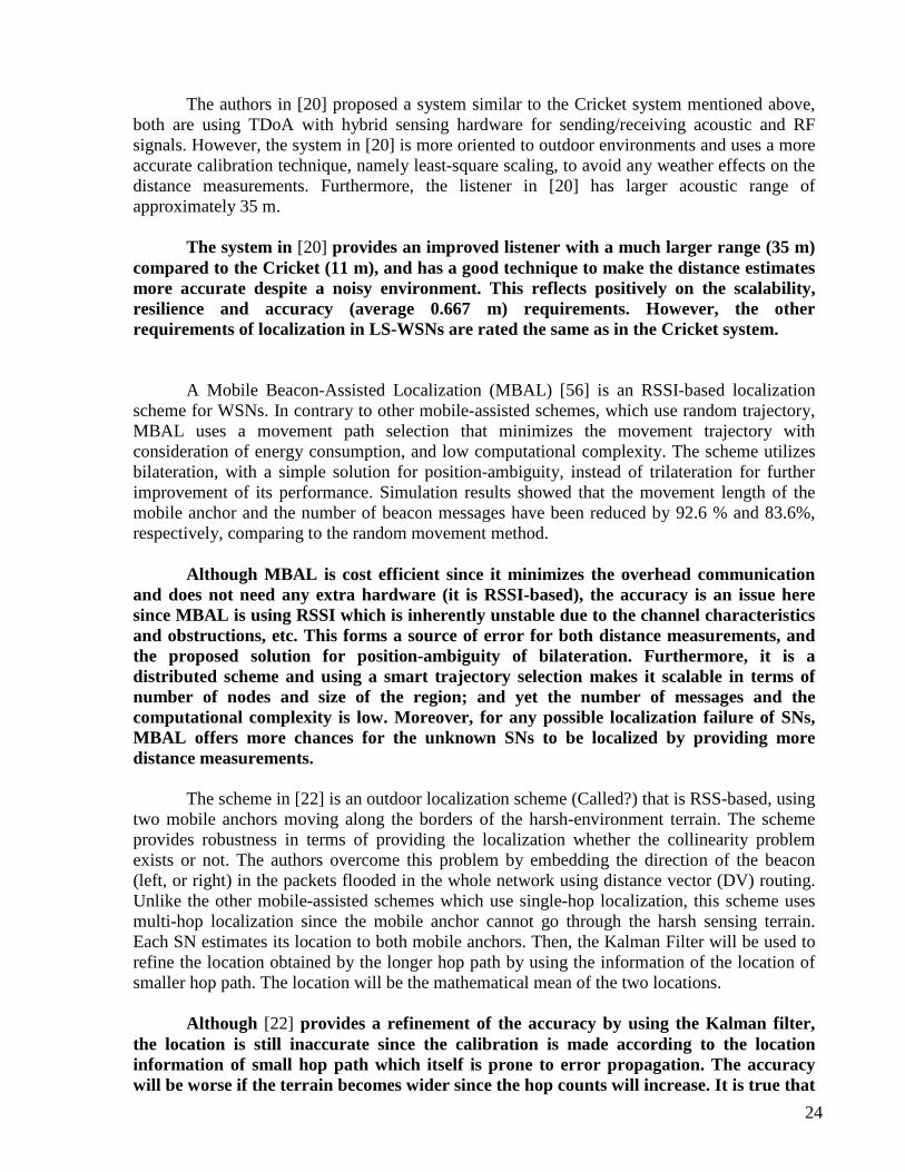
The authors in [20] proposed a system similar to the Cricket system mentioned above,

both are using TDoA with hybrid sensing hardware for sending/receiving acoustic and RF signals. However, the system in [20] is more oriented to outdoor environments and uses a more accurate calibration technique, namely least-square scaling, to avoid any weather effects on the distance measurements. Furthermore, the listener in [20] has larger acoustic range of approximately 35 m.

The system in [20] provides an improved listener with a much larger range (35 m)

compared to the Cricket (11 m), and has a good technique to make the distance estimates more accurate despite a noisy environment. This reflects positively on the scalability, resilience and accuracy (average 0.667 m) requirements. However, the other requirements of localization in LS-WSNs are rated the same as in the Cricket system.

A Mobile Beacon-Assisted Localization (MBAL) [56] is an RSSI-based localization

scheme for WSNs. In contrary to other mobile-assisted schemes, which use random trajectory, MBAL uses a movement path selection that minimizes the movement trajectory with consideration of energy consumption, and low computational complexity. The scheme utilizes bilateration, with a simple solution for position-ambiguity, instead of trilateration for further improvement of its performance. Simulation results showed that the movement length of the mobile anchor and the number of beacon messages have been reduced by 92.6 % and 83.6%, respectively, comparing to the random movement method.

Although MBAL is cost efficient since it minimizes the overhead communication

and does not need any extra hardware (it is RSSI-based), the accuracy is an issue here since MBAL is using RSSI which is inherently unstable due to the channel characteristics and obstructions, etc. This forms a source of error for both distance measurements, and the proposed solution for position-ambiguity of bilateration. Furthermore, it is a distributed scheme and using a smart trajectory selection makes it scalable in terms of number of nodes and size of the region; and yet the number of messages and the computational complexity is low. Moreover, for any possible localization failure of SNs, MBAL offers more chances for the unknown SNs to be localized by providing more distance measurements.

The scheme in [22] is an outdoor localization scheme (Called?) that is RSS-based, using

two mobile anchors moving along the borders of the harsh-environment terrain. The scheme provides robustness in terms of providing the localization whether the collinearity problem exists or not. The authors overcome this problem by embedding the direction of the beacon (left, or right) in the packets flooded in the whole network using distance vector (DV) routing. Unlike the other mobile-assisted schemes which use single-hop localization, this scheme uses multi-hop localization since the mobile anchor cannot go through the harsh sensing terrain. Each SN estimates its location to both mobile anchors. Then, the Kalman Filter will be used to refine the location obtained by the longer hop path by using the information of the location of smaller hop path. The location will be the mathematical mean of the two locations.

Although [22] provides a refinement of the accuracy by using the Kalman filter,

the location is still inaccurate since the calibration is made according to the location information of small hop path which itself is prone to error propagation. The accuracy will be worse if the terrain becomes wider since the hop counts will increase. It is true that

25

using two mobile anchors rather than using many static anchors reduces the cost, but the scheme is still flooding the packets in the whole network which increases the overhead communication, and affects also the energy efficiency. Furthermore, the scheme is distributed, but it only scales within the bounded terrain between the mobile anchors. The scheme is resilient to collinearity and any node will be localized as long as it is in the transmission range of other located node.

5.3.1.2 Angle-based Systems

In [57], the authors designed a localization scheme that relies on AoA measurements by using Omni-directional antenna array of four antennas mounted on each anchor. Each anchor starts sending omni-directional pulses and its position. Then it transmits a beacon with a rotating radiation pattern. The main direction of the beacon is changed periodically (p time period with ∆ angular changing). A sensor stores the time of the strongest beacon power. The difference in time between the receiving pulse time and the strongest beacon power allows calculating the AoA measurement of the signal. If the sensor collected AoA measurements from two or more anchors, then by using the least square method, the position of the sensor can be estimated. It was reported that six anchors were sufficient to localize 100 SNs with sensor density of one sensor per 5 m X 5m. The accuracy reported was 2-2.5 m which is acceptable.

Despite that this scheme provides good accuracy for an outdoor experiment, it

seems that it will fail getting the same accuracy for indoor environment which lacks LoS causing possible multipath fading and reflection which affects the correct reading of the anchor’s signal. The scheme is decentralized and maintains relatively low computational complexity on the sensor’s side. However, its scalability will be affected by the number of sufficient anchors since there is no collaboration and multi-hop communication between the SNs themselves. Having no multi-hop mechanism will constrain the robustness against the failure of signal reception. Furthermore, the cost of omni-directional array of antenna can be handled for small areas with limited number of anchors, but in LS-WSNs, there will be a large number of sensors over a very large area which requires many more anchors to cover the whole SNs. This will make the cost increase rapidly.

High Accuracy localization based on Angle to Landmark (HA-A2L) [58] is a

localization scheme that depends on two phases: first, design Localization Information Exchange Protocol (LIEP); and second is the localization algorithm. LIEP establishes messages (INIT, and POSITION) to exchange the localization information between the anchors and the unknown SNs as shown in Figure 12. It is assumed that each unknown SN is able to estimate the distance to its immediate neighbors and it has an antenna array to measure the AoA. In the second phase, HA-A2L uses a heuristic to control the propagation error. This heuristic trades off the number of nodes to be localized and the errors aggregated through multi-hop paths. However, this kind of trade off will increase the computational complexity for the localization scheme. The accuracy achieved is about 1 m (7%R where R=14) with network size equal to 100.

26

Figure 12. Messages exchanged by nodes in HA-A2L scheme (reproduced from [58]).

Although HA-A2L is an improved version of angle to landmark (A2L) where it

provides a good accuracy outdoors by controlling the number of hops to not exceed a threshold, it fails in the cost efficiency requirements for LS-WSNs where additional hardware (i.e. antenna array) is required and there is overhead communication by broadcasting the messages through the whole network without any smart control.

Furthermore, controlling the error propagation (by not sending more localization messages through more hops) scales down the number of nodes to be localized. The scheme is distributed, but yet consumes more energy power due to the antenna array and increases the computational complexity by applying error controlling. If the unknown SN is not localized from the first POSITION message, it has to wait until the next iteration to receive POSITION message again which is time consuming.

Ad Hoc Positioning System (APS) Using AoA [59] is a localization scheme that uses a

Distance Vector (DV) technique for routing the beacons in a hop by hop fashion. While original APS uses distance measurement to be forwarded, APS-AoA uses angle measurements to be propagated in a multi-hop manner such that even the SNs which are not in direct communication with the anchors/landmarks can still infer the estimated angle/orientation to an anchor. The estimation of the angles to an anchor can be done by using an induction-proof like process. Basic step: if the sensor is directly connected (i.e. single-hop distance) to an anchor, then it can estimate the angle to this anchor directly. The induction step: assume the sensor (say sensor s) is k-hop distance away from an anchor (say anchor A) (k>1), if its neighbors in (k-1)-hop distance have their angle measurements to anchor A, then s can estimate its angle to anchor A, and broadcast this estimated angle through the network. Triangulation method is used to estimate the location of the unknown SNs. APS-AoA is controlling the error propagated throughout the network by controlling the number of hops in such a way that minimizes the propagation error.

Although APS-AoA fulfills some requirements such as being distributed and

scaling well with increasing number of nodes, it fails in cost efficiency where additional hardware is required, and overhead signaling cost from broadcasting beacons throughout the network. The scheme is designed to work in an outdoor environment with LoS, obstructions will severely affect the angle estimation and, hence, increase the error. Furthermore, computational complexity will be increased due to applying an error control procedure which reduces the energy efficiency. Since there is a tradeoff between the coverage and accuracy, the number of hops will be constrained within a certain

27

threshold and, hence, more anchors are required to be deployed to maintain the coverage and the accuracy which increases the cost.

5.3.2 Range-free Systems The range-free technique provides coarse-grained localization since it does not depend

on calculating distances and angles unlike range-based systems. Range-free systems are either connectivity-based or fingerprint systems as explained in Section 3. We address first the localization systems that are connectivity based.

5.3.2.1 Connectivity-based Systems

DV-hop [34] is a connectivity-based range-free scheme that uses the number of hops between the SNs and three anchors to estimate the distance measurements between such sensor and these anchors. Then the triangulation method is applied to estimate the location of this SN. The approach of this scheme depends on the classical mechanism Distance Vector (DV) routing. In DV-hop, each anchor starts broadcasting beacons throughout the network. The beacon contains the anchor’s location plus the hop count which initialized to one. Each SN maintains the minimum value of hop count. Thus, if any SN (n) with current hop count (cHopCnt) receives a beacon with smaller new hop count (nHopCnt) (i.e. nHopCnt < cHopCnt) will change its current hop count value to be equal to the n’s new hop count (i.e. cHopCnt = nHopCnt). Otherwise, the beacon is dropped and the n’s current hop counter remains unchanged. Then node n will forward a beacon with hop count increased by one (i.e. cHopCnt +1). After finishing this process, all nodes (including anchors) will have the shortest path (in hops) to every anchor in the network. Then each anchor will calculate its correction factor through all other anchors by using the following formula:

2 2( ) ( ), for allanchors , .

i j i j

ii

x x y yf j j i

h

− + −= ≠∑

∑ [34]

Thus correction factor of anchor i is averaging the summation of distances between

anchor i and all other anchors over the summation of the corresponding hop counts. These correction values will be used to estimate the distance between the SN and the anchors according to the closest anchor to this sensor. For example, in Figure 13 if u is the SN and A, B, and C are the anchors with correction factors f1, f2, and f3, respectively. Then, f1= (80+120)/(5+7)=16.6 m, f2=(35+80)/(2+5)=16.4 m, and f3=(35+120)/(2+7)= 17.2 m. A is the closest anchor to u (by number of hops), then u will use the correction factor of A (i.e. f1) to estimate the distance measurements as follows: d(A, u) = f1 * hopCount1=16.6 * 2, d(B, u) = f1 * hopCount2=16.6 * 3, and d(C, u)= f1 * hopCount3=16.6 * 5, Where hopCount1, hopCount2, and hopCount3 are the distances (in hops) between u and anchors A, B, and C, respectively.

28

Figure 13. DV-hop localization scheme

Empirical tests in [33] showed that the accuracy decreases when the deployment of

the SNs is random rather than uniform. This will affect negatively the scalability of DV-hop, where usually the SNs are un-deterministically existing (either stationary or mobile) over the terrain. Also, the communication overhead increases sharply by increasing the node density. This means that DV-hop is not cost efficient despite that it does not need additional hardware. Although DV-hop poses overhead communication by broadcasting beacons to be flooded throughout the network, it is robust to beacon delivery failure since another beacon can be received from a different route. Clearly, DV-hop dos not fulfill all requirements and metrics to be a good system in LS-WSNs.

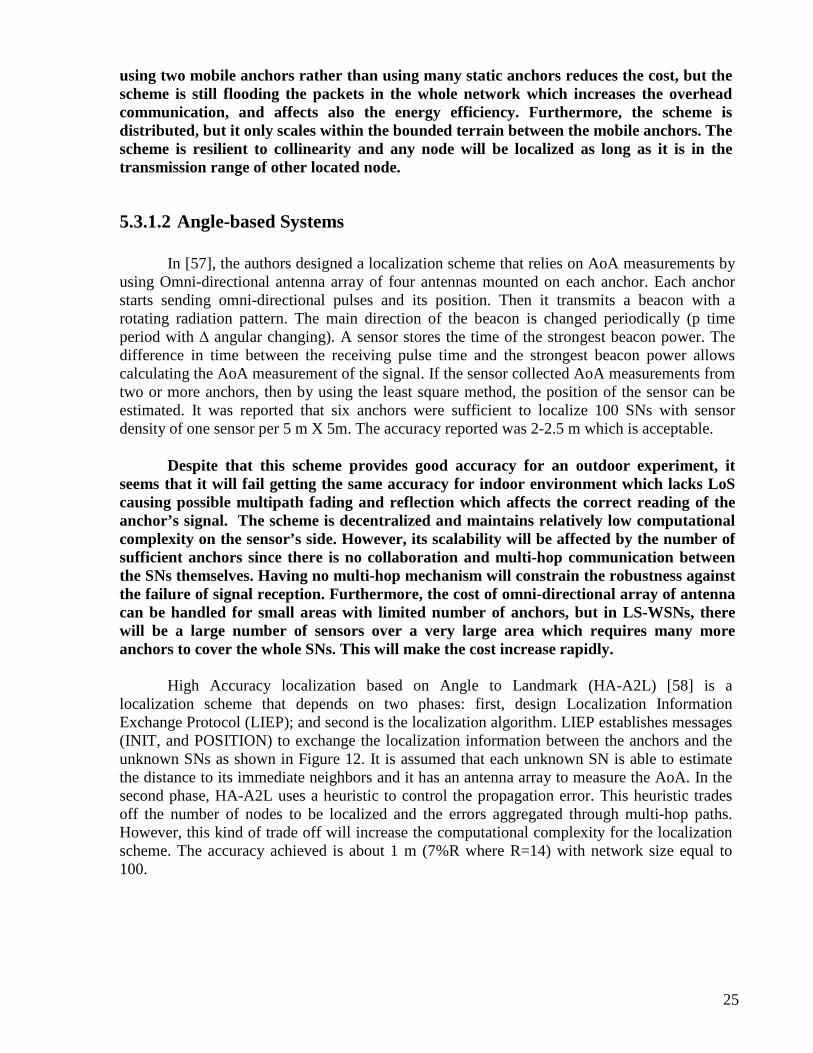
Approximate Point in Triangulation (APIT) [51] is a connectivity-based range-free

scheme that depends on Point in Triangulation (PIT) test that allows the SN to determine whether it is inside a triangle or not. This approach relays on the existence of enough anchors. Any three anchors form a triangle and by using the PIT test, the SN is either inside the triangle or not. The estimated location of the sensor is the centroid of the intersection area of all triangles containing the SN. Figure 14 shows the area-based strategy followed by APIT. The idea behind PIT test is to emulate the movement of the SN by using the local neighbors’ information. For example, the signal strength (SS) between the SNs and the anchors can be utilized to infer which sensor is closer to which anchor. By using this method, if there is no neighbor (of node A) that is closer or further from the three anchors X, Y, and Z simultaneously, then A inside the triangle XYZ. Otherwise, A is outside.

29

Figure 14. Area-based APIT Schem (reproduced from [51]).

Although APIT has good cost and energy efficiency policies, it fails to provide good

accuracy since it depends on density of anchors heard (i.e. average number of anchors used during estimation). Features like polynomial computational complexity and allowing multi-hop localization make APIT more suited for outdoor applications. Furthermore, APIT is scaling well since it is distributed, and adaptable and not sensitive to node density and size of the terrain as long as the node and anchor density remain above certain levels. Empirical tests suggest at least 6 for node degree (density) and more than 8 anchors with ANR (Anchor to Node range Ratio)5 equals to 10.

The scheme in [60] provides a mechanism to use a mobile anchor together with the In-

Range technique to localize the unknown sensors in the terrain. The mobile anchor eliminates the need to deploy many stationery expensive anchors. The trajectory of the mobile anchors follows the Random Waypoint (RWP) model. This scheme uses In-range techniques which is similar to aforementioned Point in Triangulation (PIT) in the APIT scheme where both are using the communication range of the anchors. However, PIT is using three stationary anchors to build a triangle, while [60] is using two locations of the mobile anchors and the intersection area of the two circles centered in these locations contains the location of the unknown SN. It may happen that an unknown SN is not hearing from the anchor (i.e. out of the anchor’s transmission range), yet it is in the range of another localized sensor (say A), then In-range provides extension to such an unknown SN. In this case, the location of the sensor is determined by the area that is inside the two circles centered in the vertices of A’s location area (i.e. A’s vesica piscis). In-Range technique can be iterated many times as it is required to reach the appropriate accuracy.

This scheme [60] does not require any extra hardware or overhead

communication, and uses only one mobile anchor instead of many static ones which means that it is indeed cost efficient. Furthermore, it follows a distributed manner and single-hop strategy to localize the SNs. This provides more energy efficiency and reduces the number of packets exchanged. The scheme provides full localization of the sensing field by extending the In-Range technique by using the localized SNs. However, the anchor trajectory has not been selected in a smart way to maximize the number of

5 ANR means the average distance an anchor beacon travels divided by the average distance a regular node signals travels.

30

localized sensors by the anchor itself. This will affect the accuracy and in order to make it more precise, In-Range method should be iterated many times which means more run time complexity , hence, more energy will be consumed.

5.3.2.2 Fingerprint-based Systems

RADAR [35] is a range-free fingerprint system that achieves accuracy in the range of 2-3metres. As all fingerprint (mapping) systems, RADAR has two phases of localization: construction phase (offline phase) and positioning phases (online phase). In the offline phase, RADAR synchronises the clocks of mobile host (e.g. a person carries the sensor device) and base stations (BSs). Then, the mobile host starts sending beacons (6 bytes UDP packets) every 4 seconds. In the meantime, each BS records the strength signal (SS) together with timestamp t. In other words, the tuple (t, BS, SS) is stored for each BS. The mobile host refers to its location on the map (scene) along with its direction d. This means that the tuple (t,x,y,d) is stored in each BS. Then for each tuple (x,y,d), the mean value of all SS readings for each BS is calculated. In the online phase, the actual transmitted signal strength SS from the mobile host is received by the BSs, (say three BSs), which forms the tuple (SS1, SS2, SS3) where SSi is the signal strength received by BS number i. Then it is compared to the records stored in offline phase, and the closest stored record indicates the location and direction of the mobile host. Figure 15 provides a flowchart of localization steps using RADAR scheme.

Offline Phase

• mobile host starts sending beacons .

• (t, BS, SS) is stored for each BS.

• (t,x,y,d) is recorded in each BS.

• for each (x,y,d) tuple, the mean value of all SS readings for each BS is calculated.à (SS’1, SS’2, …,SS’i) where i is the number of BSs.

Online Phase

• Actual SS is received by the BSs.• The tuple (SS1, SS2, …,SSi) is

compared to all (SS’1, SS’2, …,SS’i) in offline phase.

• the closest stored record indicates the location and direction of the mobile host. The one that minimizes the Euclidean distance with the actual tuple.

EndStart

Figure 15. RADAR phases for localization RADAR uses either empirical data or the radio propagation model to build the

database in offline phase. The radio propagation model reduces the effort and takes into consideration the obstructions (i.e. walls and floors). Thus, it is good for indoor use and provides good accuracy in the range of 2-3 metres. However, it does not provide multi-level accuracy. The information and results indicate that it is not feasible for outdoor use due to dynamic environments with moving obstructions along with large area of terrain and node density. From an energy efficiency point of view, the empirical results showed that reducing the messages by 25% (neglecting the direction issue) will not impact the behaviour of the system. Also, the computations are processed in BSs and therefore the mobile sensor devise preserves its energy. However, in real life there are many sensors have frequent RF interference which imposes an overhead cost on beacons traffic.

31

Furthermore, the system is using centralized single-hop procedure where increasing the number of sensors can still be handled by the system as long as they are able to communicate with BSs in a single-hop manner which is impractical in LS-WSNs. Using the empirical method will take a huge effort to build the data base (DB) and therefore, it is not feasible for LS-WSNs. However, using the radio propagation model will make easier to scale the terrain size, but still changing the map (scene) of the terrain by obstructions or changing the location of BS will force a re-build to the DB again. Moreover, sending more than one message from the same location is a policy to guarantee more messages to reach the BSs, but there are no policies to deal with other kinds of failures. Clearly, RADAR met some localization requirements in LS-WSNs, but fails in most of them.

Error Controlling LOCAlizaTION scheme (Ecolocation) [61] uses the Radio Signal

Strength (RSS) to estimate the location of the unknown SN. The terrain, where the anchor nodes and SNs are deployed, is divided into grid-point locations. Each grid-point location calculates the Euclidian distance measures to all anchors. In an ideal case (zero multipath fading and shadowing), the closer the anchor is to the SN, the larger the RSS will be from this SN; and this is called constraint. Based on this key idea, each grid-point location will have its own set of (ideal) constraints by ordering the anchors in its communication range from closer to further (i.e. high RSS to low RSS). The localization process starts by the unknown SNs which broadcast a beacon to anchors. Each (hearing) anchor will send its RSS to a specific node point (i.e. cluster head or any other node with good computational capability); at this point, the collected RSSs are used to form an ordered sequence of anchors (i.e. set of constraints). This set of constraints will be compared with all sets of constraints of grid-point locations; and then pick the location that maximizes the number of matched constraints. If there is more than one location which has the same maximum number of matched constraints, then the estimated position for the SN will be the centroid of these locations.

Although Echolocation is a robust scheme to multi-path effects of the RF channel

by using the distance-based rank ordering of the anchors as a unique signature in the localization process, it fails in critical requirements like scalability since it depends on grid layout which is impractical in LS-WSNs. The accuracy of Ecolocation depends on RF channel characteristics (i.e. path loss and standard deviation), and number of anchor nodes. The experiments showed that it provided better accuracy (with increasing number of anchors, path loss and/or decreasing the standard deviation) compared to other schemes such as the proximity scheme. However, the experiments used single-hop communication between the SN and the anchors to measure the accuracy, which is not usually the case in LS-WSNs. That is why we believe that the accuracy will be diminished due to the error propagation through the network. Furthermore, the computational complexity of Ecolocation depends on the size of the terrain, the number of anchors and the number of grid points which will be computationally costly for LS-WSNs and especially if the SNs are mobile rather than static as in Ecolocation.

Location Identification based on Dynamic Active RFID Calibration (LANDMARC)

[36] is a system that employs fixed active RFID tags as references/anchors along with RFID readers to help in location calibration and thus enhance the accuracy. The idea is to replace the cheaper active RFID instead of the expensive RFID readers. While current RFID systems do not provide the signal strength of tags directly to reader6, LANDMARC reflects the relation between the power level and signal strength. So LANDMARC requires the signal strengths of

6 RFID reader receives the power level of the tag detected

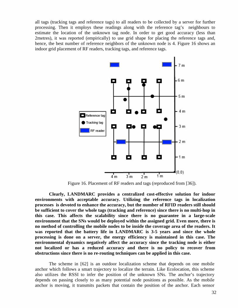
32

all tags (tracking tags and reference tags) to all readers to be collected by a server for further processing. Then it employs these readings along with the reference tag’s neighbours to estimate the location of the unknown tag node. In order to get good accuracy (less than 2metres), it was reported (empirically) to use grid shape for placing the reference tags and, hence, the best number of reference neighbors of the unknown node is 4. Figure 16 shows an indoor grid placement of RF readers, tracking tags, and reference tags.

Figure 16. Placement of RF readers and tags (reproduced from [36]).

Clearly, LANDMARC provides a centralized cost-effective solution for indoor

environments with acceptable accuracy. Utilizing the reference tags in localization processes is devoted to enhance the accuracy, but the number of RFID readers still should be sufficient to cover the whole tags (tracking and reference) since there is no multi-hop in this case. This affects the scalability since there is no guarantee in a large-scale environment that the SNs would be deployed within the assigned grid. Even more, there is no method of controlling the mobile nodes to be inside the coverage area of the readers. It was reported that the battery life in LANDMARC is 3-5 years and since the whole processing is done on a server, the energy efficiency is maintained in this case. The environmental dynamics negatively affect the accuracy since the tracking node is either not localized or has a reduced accuracy and there is no policy to recover from obstructions since there is no re-routing techniques can be applied in this case.

The scheme in [62] is an outdoor localization scheme that depends on one mobile

anchor which follows a smart trajectory to localize the terrain. Like Ecolocation, this scheme also utilizes the RSSI to infer the position of the unknown SNs. The anchor’s trajectory depends on passing closely to as many potential node positions as possible. As the mobile anchor is moving, it transmits packets that contain the position of the anchor. Each sensor

33

receiving the packet constructs a constraint on its location estimate. This constraint considers the bounding coordinates for the terrain and the idea that states “As the distance increases, the RSSI decreases and vice versa (normal conditions)” [REF]. Then the Bayesian inference and weighted average is applied in each SN to estimate the positions of the SNs.

This scheme [62] requires no extra hardware and has no overhead communication,

but some effort would be made to figure out bounding coordinates of the deployment area in order to use them in evaluating the constraints. Regarding accuracy, this scheme requires prior evaluation of environment data for calibration to give more precision of the localization results. However, it does not provide multi-level accuracy and its performance indoor is expected to be poor due to the obstructions and multipath. Furthermore, this scheme is single-hop and has a low computational complexity since each node will calculate simple formulas. Moreover, the scheme is distributed and scaled well inside the area of deployment. However, extending the area requires re-evaluating the bounding coordinates and may need data re-calibration if the environment changed in the new extended terrain. Finally, the robustness depends on the mobile anchor to cover the whole area; if the SN did not receive (or receive bad) packets, then there is no designated policy to localize it again.

At this point, we complete the analysis of classified localization schemes and systems

on the light of LS-WSNs requirements. Table 5 shows the summary of the performance evaluation.

34

Table 5. The performance evaluation of classified localization schemes and systems against LS-WSNs metrics

Localization Technique

Type Scheme/ System

Environment Mobile (M)/

Static (S) Anchors

Single-/Multi- hops

Accuracy Energy

Efficiency Scalability Resilience

Cost Efficiency

Ra

ng

e-b

ase

d

Dis

tan

ce-b

ase

d

GPS Outdoor M Single Moderate Poor Moderate Moderate Moderate

Cricket Indoor S Single Moderate Moderate Moderate Poor Moderate

[20] Outdoor S Single Moderate Moderate Moderate Moderate Moderate

MBAL Outdoor M Single Moderate Good Good Good Good

[22] Outdoor M Multiple Poor Moderate Moderate Good Moderate

An

gle

-ba

sed [57] Outdoor S Single Moderate Good Moderate Moderate Moderate

HA-A2L Outdoor S Multiple Moderate Moderate Moderate Moderate Poor

APS-AoA Outdoor S Single Moderate Moderate Moderate Moderate Poor

Ra

ng

e-f

ree Co

nn

ect

ivity

–b

ase

d

DV-hop Outdoor S Multiple Moderate Moderate Moderate Good Moderate

APIT Outdoor S Single Moderate Good Good Good Good

[60] Outdoor M Single Moderate Moderate Good Good Good

Fin

ge

rpri

nt

RADAR Indoor S Single Moderate Moderate Moderate Moderate Good

Ecolocation Outdoor/Indoor

S Single Moderate Moderate Poor Moderate Good

LANDMARC Indoor S Single Moderate Good Poor Poor Good

[62] Outdoor M Single Moderate Good Moderate Moderate Moderate

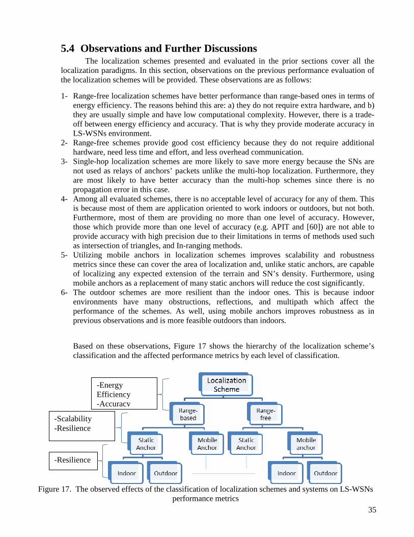
35

5.4 Observations and Further Discussions The localization schemes presented and evaluated in the prior sections cover all the

localization paradigms. In this section, observations on the previous performance evaluation of the localization schemes will be provided. These observations are as follows:

1- Range-free localization schemes have better performance than range-based ones in terms of energy efficiency. The reasons behind this are: a) they do not require extra hardware, and b) they are usually simple and have low computational complexity. However, there is a trade-off between energy efficiency and accuracy. That is why they provide moderate accuracy in LS-WSNs environment.

2- Range-free schemes provide good cost efficiency because they do not require additional hardware, need less time and effort, and less overhead communication.

3- Single-hop localization schemes are more likely to save more energy because the SNs are not used as relays of anchors’ packets unlike the multi-hop localization. Furthermore, they are most likely to have better accuracy than the multi-hop schemes since there is no propagation error in this case.

4- Among all evaluated schemes, there is no acceptable level of accuracy for any of them. This is because most of them are application oriented to work indoors or outdoors, but not both. Furthermore, most of them are providing no more than one level of accuracy. However, those which provide more than one level of accuracy (e.g. APIT and [60]) are not able to provide accuracy with high precision due to their limitations in terms of methods used such as intersection of triangles, and In-ranging methods.

5- Utilizing mobile anchors in localization schemes improves scalability and robustness metrics since these can cover the area of localization and, unlike static anchors, are capable of localizing any expected extension of the terrain and SN’s density. Furthermore, using mobile anchors as a replacement of many static anchors will reduce the cost significantly.

6- The outdoor schemes are more resilient than the indoor ones. This is because indoor environments have many obstructions, reflections, and multipath which affect the performance of the schemes. As well, using mobile anchors improves robustness as in previous observations and is more feasible outdoors than indoors.

Based on these observations, Figure 17 shows the hierarchy of the localization scheme’s classification and the affected performance metrics by each level of classification.

Figure 17. The observed effects of the classification of localization schemes and systems on LS-WSNs performance metrics

-Energy Efficiency -Accuracy

-Scalability -Resilience

-Resilience

36

According to our observations and the current resource limitations of the SNs, there is always a kind of trade-off between accuracy and energy consumption. In other words, focusing on high accuracy requires range-based technique which, usually, requires extra hardware (i.e. increasing cost), and requires more energy (i.e. increasing energy consumption), which, in turn, affects negatively the scalability and resilience (i.e. reducing the scalability and resilience). Therefore, it is better to design a localization scheme to fit many applications in terms of multi-level accuracy. However, this will require extra hardware that can be utilized when high accuracy is desired. Otherwise, other methods, which do not require extra hardware such as RSSI, can be used to achieve acceptable levels of accuracy.

While energy efficiency is very important metric in assessing localization schemes and systems especially in large-scale environment, it is time and effort worthy to create a filtering criterion based on this metric before doing the full performance analysis of these schemes. This filtering criterion (i.e. energy efficiency) is well-defined to filter the schemes and systems precisely. Indeed there are no schemes that will fit the large-scale localization with high energy consumption. In other words, the energy resources will be depleted before localizing the entire number of nodes in the network. Thus, we propose two phases to assess these schemes/systems, namely selection/fitness phase and refinement phases. The filtering phase is some kind of breadth evaluation where the filtering criterion will be applied on the schemes to determine whether the scheme fits the large-scale localization or not. Then in the refinement phase, which is a depth evaluation, the filtered systems will be evaluated against the defined features of metrics as shown in the previous section. In this regard, the schemes that perform poorly in energy efficiency will be marked as “unfit” and, therefore, no need for further evaluating (i.e. no need to apply phase two). For example, scheme number one in Table 5, namely GPS, will be unfit and will not be handled in phase two because of its poor performance in the filtering criterion.

Two questions are raised here about the schemes and systems presented in Table 5:

a) What are the recommended schemes for localization in LS-WSNs?

b) What are the suggested enhancements for such schemes?

There are two promising schemes among all schemes in Table 5, namely MBAL and APIT, which can be enhanced to perform well in LS-WSNs. Both of them are performing well in all metrics except the accuracy. In our prior evaluation, MBAL is an outdoor distance-based scheme that has no multi-level accuracy. Therefore, MBAL can be enhanced in such a way that it provides more than on level of accuracy and have the ability to utilize the infrastructure indoor. This can be achieved by embedding extra hardware to utilize other methods, rather than its RSSI method, like ToA or TDoA for better desired accuracy. In this way, the scheme will not use this hardware until the application requires high accuracy. Since mobile anchors are not feasible indoors, MBAL should be adjusted to work with static anchors placed inside buildings.

APIT provides multi-level accuracy but cannot provide high accuracy due to range-free method. The enhancement can be to focus on hybrid model by using range-based technique like RSSI to improve the accuracy further. For even greater accuracy, additional hardware is required to utilize ToA or TDoA. Also, dense static anchors should be deployed to maintain the resilience and acceptable level of accuracy especially indoor environment.

37

6 Summary and Open Research Problems

In the following subsections, a summary of this paper and open research problems will be presented.

6.1 Summary This paper surveys various existing localization schemes and systems. It provides a new

classification of these schemes and investigates the characteristics, and challenges of localization in LS-WSNs. This paper also studies the requirements of localization schemes in LS-WSNs environment. According to these requirements, well defined and suitable metrics are designed to evaluate the performance of the existing localization schemes and systems in LS-WSNs environment. Observations and suggestions are also provided in the light of the qualitative comparisons of these schemes and systems.

6.2 Open Research Problems Future trends of localization in LS-WSNs may include the following: a) Multi-modal or hybrid localization schemes are required more than before to fulfill the

requirements of large-scale environments. This will allow using more than one technique in the same scheme. For example, use RSSI and ToA to achieve the best features in both and have the ability to alternate between them according to the required purpose (e.g. good level of accuracy).

b) Study all types of errors generated by measurements or propagation is very urgent these times. Such study should provide full characteristics of various types of errors and suggest ways and methods to control them. Thus, new ideas will come up about multi-hop localization, mobile anchor trajectory selection and static anchor placement. This will be very helpful in designing good localization schemes for large-scale environments.

c) There is a need for a study of integrating the existing schemes and systems in such a way that the best features in each of them can be fully utilized. For example, good outdoor scheme (e.g. MBAL) can be interworked with another indoor scheme (e.g. RADAR) to provide indoor/outdoor localization.

d) Standardization of localization in WSNs and then in LS-WSNs is required in order to design and measure all schemes using the same baseline. This will simplify the procedure of building localization systems for LS-WSNs and perform comparisons and simulations to assess which of them will be better for a specific kind of application.

e) What is the impact of the mobility of both sensor and anchor nodes on the localization process? Which metrics in LS-WSNs will be affected positively, and to what extent, by utilizing the mobility feature?

38

References

[1] I. F. Akyildiz, W. Su, Y. Sankarasubramaniam and E. Cayirci. A survey on sensor networks. Communications Magazine, IEEE 40(8), pp. 102-114. 2002.

[2] C. S. Raghavendra, K. M. Sivalingam and T. Znati. Wireless Sensor Networks 2006.

[3] N. Fallah, I. Apostolopoulos, K. Bekris and E. Folmer, "Indoor Human Navigation Systems: A Survey," Interact Comput, vol. 25, pp. 21-33, 2013.

[4] N. Xu. A survey of sensor network applications. IEEE Communications Magazine 40(8), pp. 102-114. 2002.

[5] J. Wang, R. Ghosh and S. K. Das, "A survey on sensor localization," Journal of Control Theory and Applications, vol. 8, pp. 2-11, 2010.

[6] Y. Pei. A survey on localization algorithms for wireless ad hoc networks. Communications and Information Processing pp. 512-519. 2012.

[7] I. Amundson and X. Koutsoukos. A survey on localization for mobile wireless sensor networks. Mobile Entity Localization and Tracking in GPS-Less Environments pp. 235-254. 2009.

[8] I. A. Getting, "Perspective/navigation-the global positioning system," Spectrum, IEEE, vol. 30, pp. 36-38, 1993.

[9] F. Mourad, H. Snoussi, F. Abdallah and C. Richard. Anchor-based localization via interval analysis for mobile ad-hoc sensor networks. IEEE Transactions on Signal Processing 57(8), pp. 3226. 2009.

[10] K. F. Ssu, C. H. Ou and H. C. Jiau. Localization with mobile anchor points in wireless sensor networks. Vehicular Technology, IEEE Transactions on 54(3), pp. 1187-1197. 2005.

[11] N. B. Priyantha, H. Balakrishnan, E. Demaine and S. Teller. Anchor-free distributed localization in sensor networks. Presented at Proceedings of the 1st International Conference on Embedded Networked Sensor Systems. 2003.

[12] N. Bulusu, D. Estrin, L. Girod and J. Heidemann. Scalable coordination for wireless sensor networks: Self-configuring localization systems. Presented at International Symposium on Communication Theory and Applications (ISCTA 2001), Ambleside, UK. 2001.

[13] N. Bulusu, J. Heidemann, D. Estrin and T. Tran. Self-configuring localization systems: Design and experimental evaluation. ACM Transactions on Embedded Computing Systems (TECS) 3(1), pp. 24-60. 2004.

[14] G. Deak, K. Curran and J. Condell. A survey of active and passive indoor localisation systems. Comput. Commun. 2012.

39

[15] U. B. Ceipidor, M. Dibitonto, L. D’Ascenzo and C. M. Medaglia. Localization issues in a ZigBee based internet of things scenario. The Internet of Things pp. 157-165. 2010.

[16] Y. Gu, A. Lo and I. Niemegeers. A survey of indoor positioning systems for wireless personal networks. Communications Surveys & Tutorials, IEEE 11(1), pp. 13-32. 2009.

[17] C. S. J. Rabaey and K. Langendoen. Robust positioning algorithms for distributed ad-hoc wireless sensor networks. Presented at USENIX Technical Annual Conference. 2002.

[18] L. Galluccio, G. Morabito and S. Palazzo. On the potentials of object group localization in the internet of things. Presented at World of Wireless, Mobile and Multimedia Networks (WoWMoM), 2011 IEEE International Symposium on a. 2011.

[19] X. Cheng, A. Thaeler, G. Xue and D. Chen. TPS: A time-based positioning scheme for outdoor wireless sensor networks. Presented at INFOCOM 2004. Twenty-Third AnnualJoint Conference of the IEEE Computer and Communications Societies. 2004.

[20] Y. Kwon, K. Mechitov, S. Sundresh, W. Kim and G. Agha. Resilient localization for sensor networks in outdoor environments. Presented at Distributed Computing Systems, 2005. ICDCS 2005. Proceedings. 25th IEEE International Conference on. 2005.

[21] W. M. Ibrahim, A. Taha and H. S. Hassanein, "Scalability issues in localizing things," in Local Computer Networks (LCN), 2011 IEEE 36th Conference on, 2011, pp. 673-680.

[22] W. M. Ibrahim, A. M. Taha and H. S. Hassanein, "Robust wireless multihop localization using mobile anchors," in IEEE ICC 2013- Ad-Hoc and Sensor Networking Symposium, Budapest, Hungary, 2013, pp. 99-104.

[23] L. Lazos and R. Poovendran. HiRLoc: High-resolution robust localization for wireless sensor networks. Selected Areas in Communications, IEEE Journal on 24(2), pp. 233-246. 2006.

[24] L. Lazos and R. Poovendran. SeRLoc: Robust localization for wireless sensor networks. ACM Transactions on Sensor Networks (TOSN) 1(1), pp. 73-100. 2005.

[25] H. Liu, H. Darabi, P. Banerjee and J. Liu. Survey of wireless indoor positioning techniques and systems. Systems, Man, and Cybernetics, Part C: Applications and Reviews, IEEE Transactions on 37(6), pp. 1067-1080. 2007.

[26] Y. Z. Z. Baoyu, "A Survey on Wireless Sensor Networks," Computer Engineering and Applications, vol. 15, pp. 007, 2005.

[27] M. Ilyas and I. Mahgoub. Handbook of Sensor Networks: Compact Wireless and Wired Sensing Systems 2004.

[28] U. Nazir, N. Shahid, M. Arshad and S. Raza, "Classification of localization algorithms for wireless sensor network: A survey," in Open Source Systems and Technologies (ICOSST), 2012 International Conference on, 2012, pp. 1-5.

40

[29] K. Akkaya and M. Younis. A survey on routing protocols for wireless sensor networks. Ad Hoc Networks 3(3), pp. 325-349. 2005.

[30] H. Karl and A. Willig. Protocols and Architectures for Wireless Sensor Networks 2007.

[31] F. Franceschini, M. Galetto, D. Maisano and L. Mastrogiacomo. A review of localization algorithms for distributed wireless sensor networks in manufacturing. Int. J. Comput. Integr. Manuf. 22(7), pp. 698-716. 2009.

[32] W. Dargie and C. Poellabauer, Fundamentals of Wireless Sensor Networks: Theory and Practice. Wiley. com, 2010.

[33] T. He, C. Huang, B. M. Blum, J. A. Stankovic and T. F. Abdelzaher. Range-free localization and its impact on large scale sensor networks. ACM Transactions on Embedded Computing Systems (TECS) 4(4), pp. 877-906. 2005.

[34] D. Niculescu and B. Nath. DV based positioning in ad hoc networks. Telecommunication Systems 22(1), pp. 267-280. 2003.

[35] P. Bahl and V. N. Padmanabhan. RADAR: An in-building RF-based user location and tracking system. Presented at INFOCOM 2000. Nineteenth Annual Joint Conference of the IEEE Computer and Communications Societies. Proceedings. IEEE. 2000.

[36] L. M. Ni, Y. Liu, Y. C. Lau and A. P. Patil. LANDMARC: Indoor location sensing using active RFID. Wireless Networks 10(6), pp. 701-710. 2004.

[37] G. Mao, B. Fidan and B. Anderson. Wireless sensor network localization techniques. Computer Networks 51(10), pp. 2529-2553. 2007.

[38] X. Qu and L. Xie, "A comparison study on TDOA based localization algorithms for sensor networks." 2013.

[39] G. Han, J. Jiang, L. Shu, Y. Xu and F. Wang, "Localization algorithms of underwater wireless sensor networks: A survey," Sensors, vol. 12, pp. 2026-2061, 2012.

[40] I. Guvenc and C. C. Chong. A survey on TOA based wireless localization and NLOS mitigation techniques. Communications Surveys & Tutorials, IEEE 11(3), pp. 107-124. 2009.

[41] K. Whitehouse, C. Karlof and D. Culler. A practical evaluation of radio signal strength for ranging-based localization. ACM SIGMOBILE Mobile Computing and Communications Review 11(1), pp. 41-52. 2007.

[42] P. Rong and M. L. Sichitiu. Angle of arrival localization for wireless sensor networks. Presented at Sensor and Ad Hoc Communications and Networks, 2006. SECON'06. 2006 3rd Annual IEEE Communications Society on. 2006.

[43] A. Savvides, C. C. Han and M. B. Strivastava. Dynamic fine-grained localization in ad-hoc networks of sensors. Presented at International Conference on Mobile Computing and

41

Networking: Proceedings of the 7 Th Annual International Conference on Mobile Computing and Networking. 2001.

[44] K. Langendoen and N. Reijers. Distributed localization in wireless sensor networks: A quantitative comparison. Computer Networks 43(4), pp. 499-518. 2003.

[45] G. S. Kuruoglu, M. Erol and S. Oktug. Localization in wireless sensor networks with range measurement errors. Presented at Telecommunications, 2009. AICT'09. Fifth Advanced International Conference on. 2009.

[46] H. P. Tan, R. Diamant, W. K. G. Seah and M. Waldmeyer. A survey of techniques and challenges in underwater localization. Ocean Eng. 38(14), pp. 1663-1676. 2011.

[47] T. Wu, G. Liaw, S. Huang, W. Lee and C. Wu, "A GA-based mobile RFID localization scheme for internet of things," Personal and Ubiquitous Computing, vol. 16, pp. 245-258, 2012.

[48] F. Seco, A. R. Jiménez, C. Prieto, J. Roa and K. Koutsou. A survey of mathematical methods for indoor localization. Presented at Intelligent Signal Processing, 2009. WISP 2009. IEEE International Symposium on. 2009.

[49] Z. Chen, F. Xia, T. Huang, F. Bu and H. Wang. A localization method for the internet of things. The Journal of Supercomputing pp. 1-18. 2012.

[50] X. Shen, Z. Wang, P. Jiang, R. Lin and Y. Sun. Connectivity and RSSI based localization scheme for wireless sensor networks. Advances in Intelligent Computing pp. 578-587. 2005.

[51] T. He, C. Huang, B. M. Blum, J. A. Stankovic and T. Abdelzaher. Range-free localization schemes for large scale sensor networks. Presented at Proceedings of the 9th Annual International Conference on Mobile Computing and Networking. 2003.

[52] Z. Zhou, J. H. Cui and S. Zhou. Localization for large-scale underwater sensor networks. NETWORKING 2007.Ad Hoc and Sensor Networks, Wireless Networks, Next Generation Internet pp. 108-119. 2007.

[53] G. Mao and B. Fidan. Localization Algorithms and Strategies for Wireless Sensor Networks 2009.

[54] N. B. Priyantha, H. Balakrishnan, E. D. Demaine and S. Teller. Mobile-assisted localization in wireless sensor networks. Presented at INFOCOM 2005. 24th Annual Joint Conference of the IEEE Computer and Communications Societies. Proceedings IEEE. 2005.

[55] N. B. Priyantha, A. Chakraborty and H. Balakrishnan. The cricket location-support system. Presented at Proceedings of the 6th Annual International Conference on Mobile Computing and Networking. 2000.

42

[56] K. Kim and W. Lee, "MBAL: A mobile beacon-assisted localization scheme for wireless sensor networks," in Computer Communications and Networks, 2007. ICCCN 2007. Proceedings of 16th International Conference on, 2007, pp. 57-62.

[57] P. Kułakowski, J. Vales-Alonso, E. Egea-López, W. Ludwin and J. García-Haro. Angle-of-arrival localization based on antenna arrays for wireless sensor networks. Comput. Electr. Eng. 36(6), pp. 1181-1186. 2010.

[58] M. Boushaba, A. Hafid and A. Benslimane, "High accuracy localization method using AoA in sensor networks," Computer Networks, vol. 53, pp. 3076-3088, 2009.

[59] D. Niculescu and B. Nath. Ad hoc positioning system (APS) using AOA. Presented at INFOCOM 2003. Twenty-Second Annual Joint Conference of the IEEE Computer and Communications. IEEE Societies. 2003.

[60] T. Srinath, "Localization in resource constrained sensor networks using a mobile beacon with in-ranging," in Wireless and Optical Communications Networks, 2006 IFIP International Conference on, 2006, pp. 5 pp.-5.

[61] K. Yedavalli, B. Krishnamachari, S. Ravula and B. Srinivasan. Ecolocation: A sequence based technique for RF localization in wireless sensor networks. Presented at Proceedings of the 4th International Symposium on Information Processing in Sensor Networks. 2005.

[62] M. L. Sichitiu and V. Ramadurai. Localization of wireless sensor networks with a mobile beacon. Presented at Mobile Ad-Hoc and Sensor Systems, 2004 IEEE International Conference on. 2004.